
Efficient Mathematical Lower Bounds for City Logistics Distribution Network with Intra-Echelon Connection of Facilities: Bridging the Gap from Theoretical Model Formulations to Practical Solutions

Abstract
1. Introduction
- (1)
- Increased efficiency: By breaking down the original problem into smaller subproblems, the algorithm can reduce the overall computational complexity of the optimization problem. This can lead to faster solution times and increased efficiency compared to traditional optimization algorithms.
- (2)
- Improved scalability: The algorithm can handle large-scale optimization problems that would be intractable using other methods. Large problems can be decomposed into smaller subproblems that can be solved independently, which makes it easier to solve the overall problem.
- (3)
- Better quality solutions: Since the algorithms combine both exact and heuristic methods, they are able to find high-quality solutions that balance feasibility and optimality. Some subproblems may be solved exactly while others may use heuristic methods to find good approximate solutions.
- (4)
- Robustness: Since the algorithms are designed to handle complex real-world problems, they are often more robust than traditional optimization algorithms. This means that they can handle uncertain or variable inputs and can adapt to changing conditions or constraints during the optimization process.
2. Literature Review
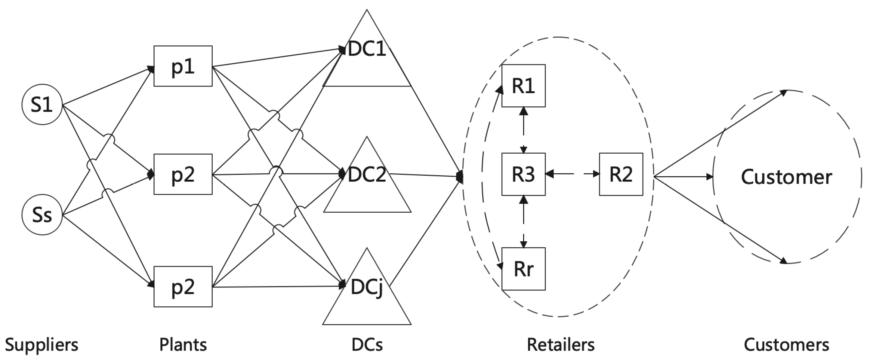
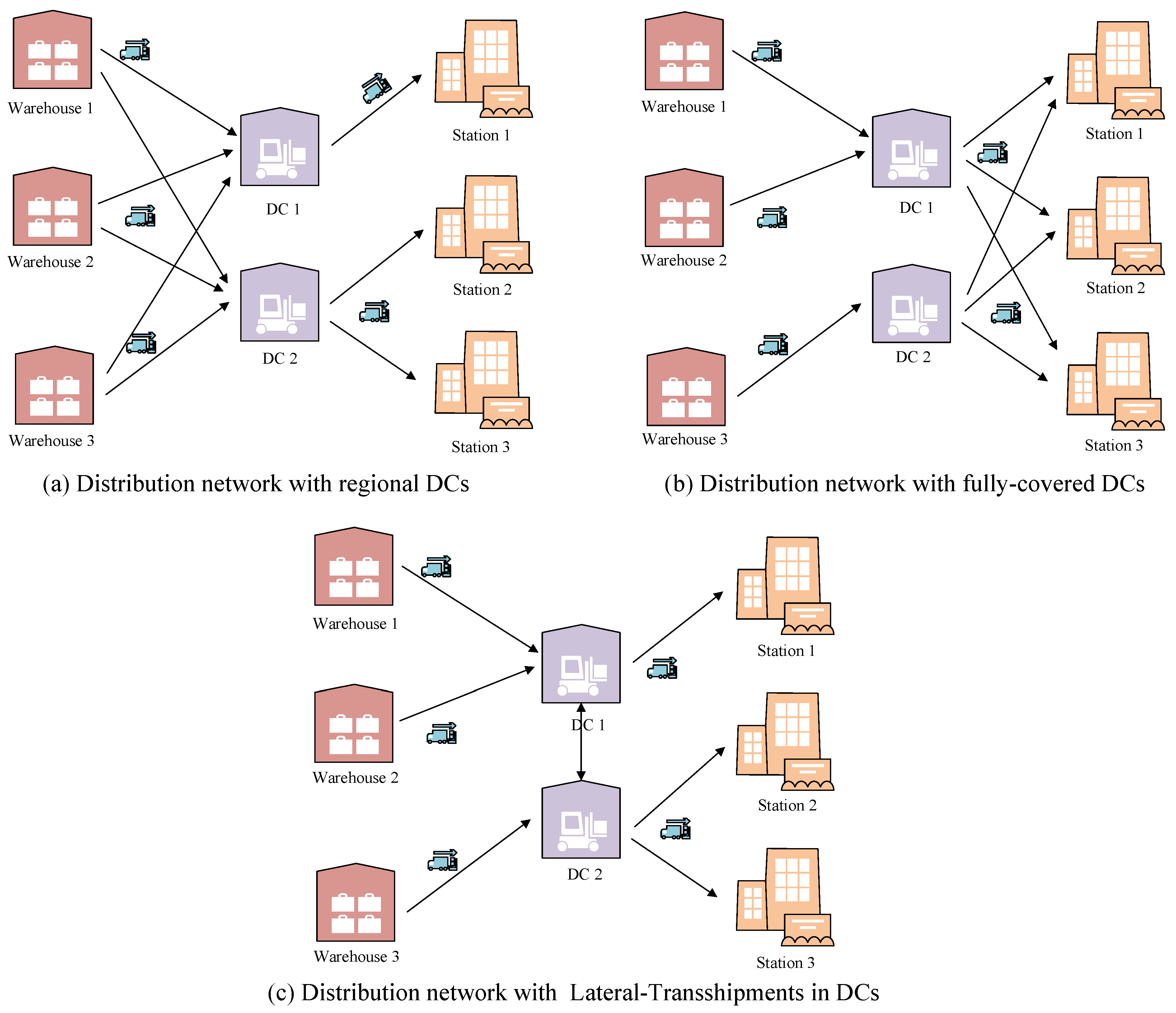
2.1. Basic Types of City Logistics Distribution Networks
2.2. Distribution Network Design Problem and Related Models
2.3. Solution Algorithms
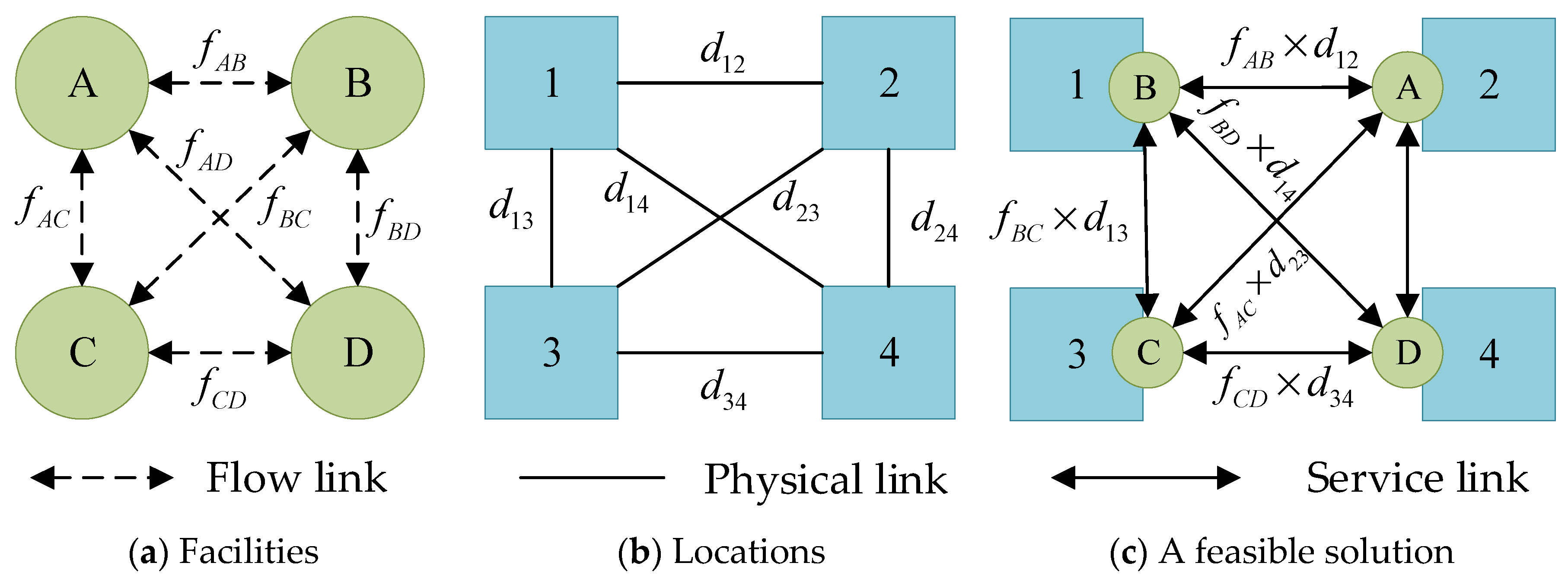
3. Problem Description and Formulation
3.1. Problem Description
- (1)
- A single sourcing/single path strategy [17] assumes that each warehouse can only be assigned to a single DC and one station can only be covered by one DC.
- (2)
- (3)
- Transportation cost is expressed as a piecewise linear function of material flow [50] and it is proportional to the volume of freight flows (i.e., transportation costs equal to the product of distance and freight flows in our problem).
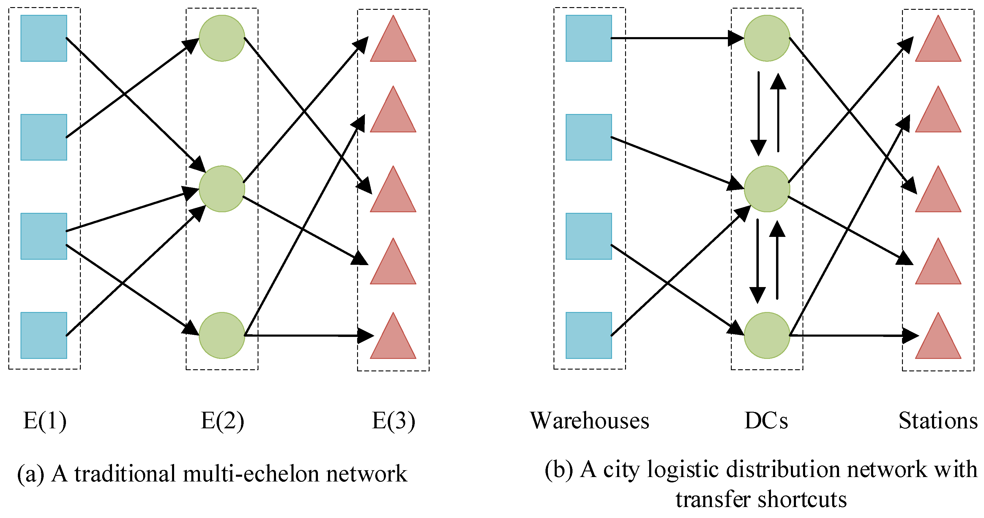
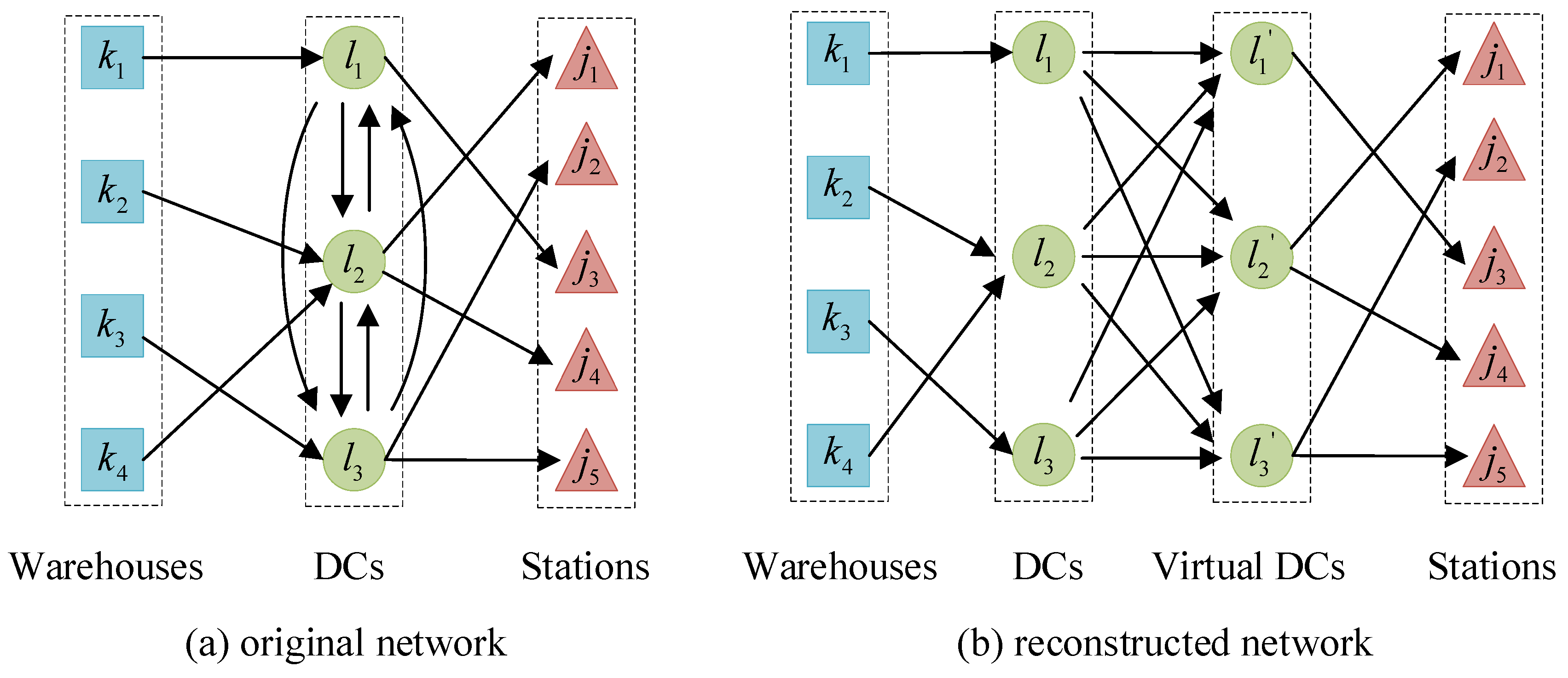
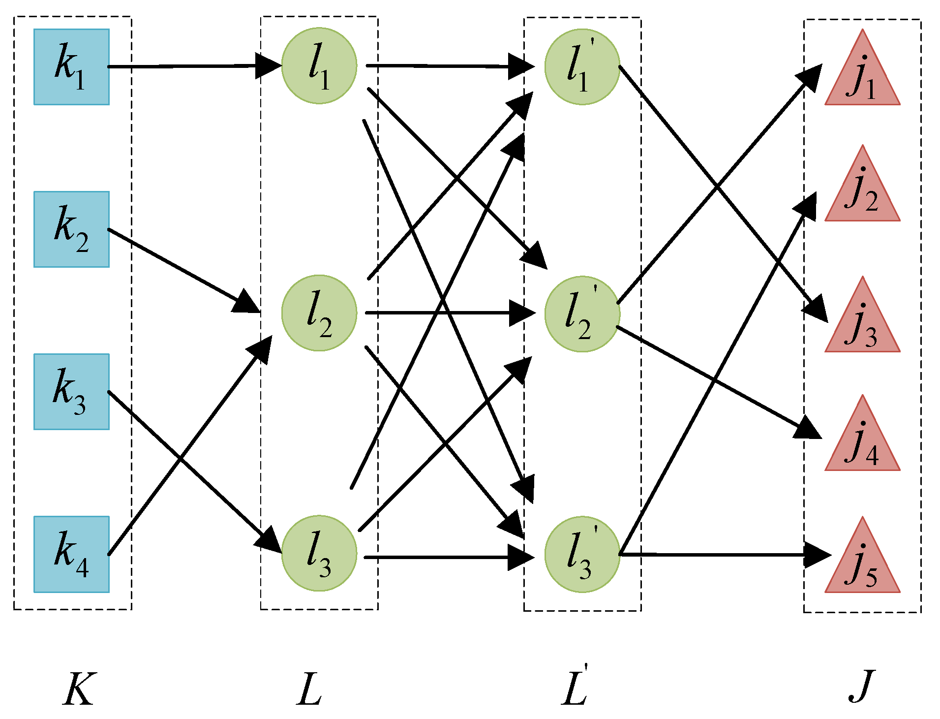
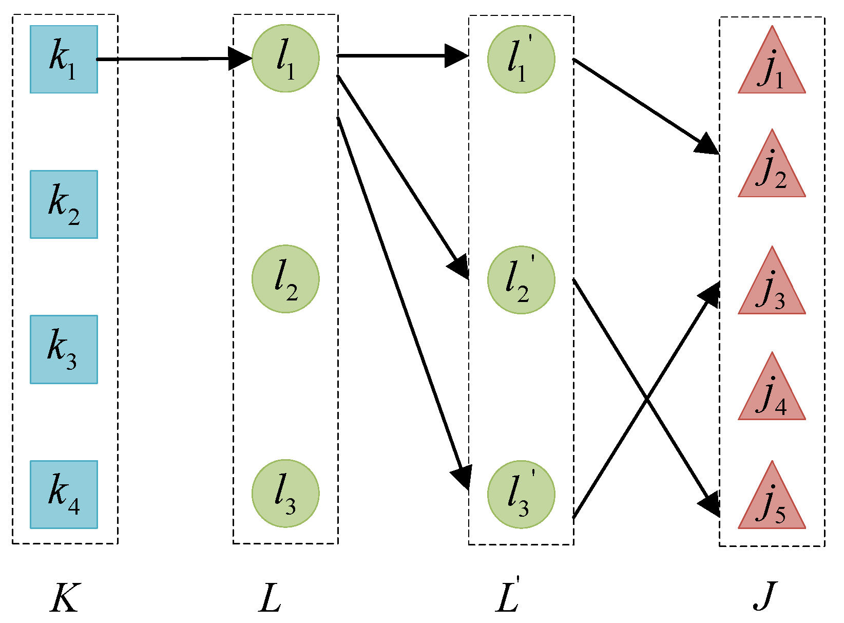
3.2. Network Model Construction for Logistics Network with Shortcuts
3.3. Quadratic Semi-Assignment Model M1 with Capacity Constraints
4. Solution Algorithms
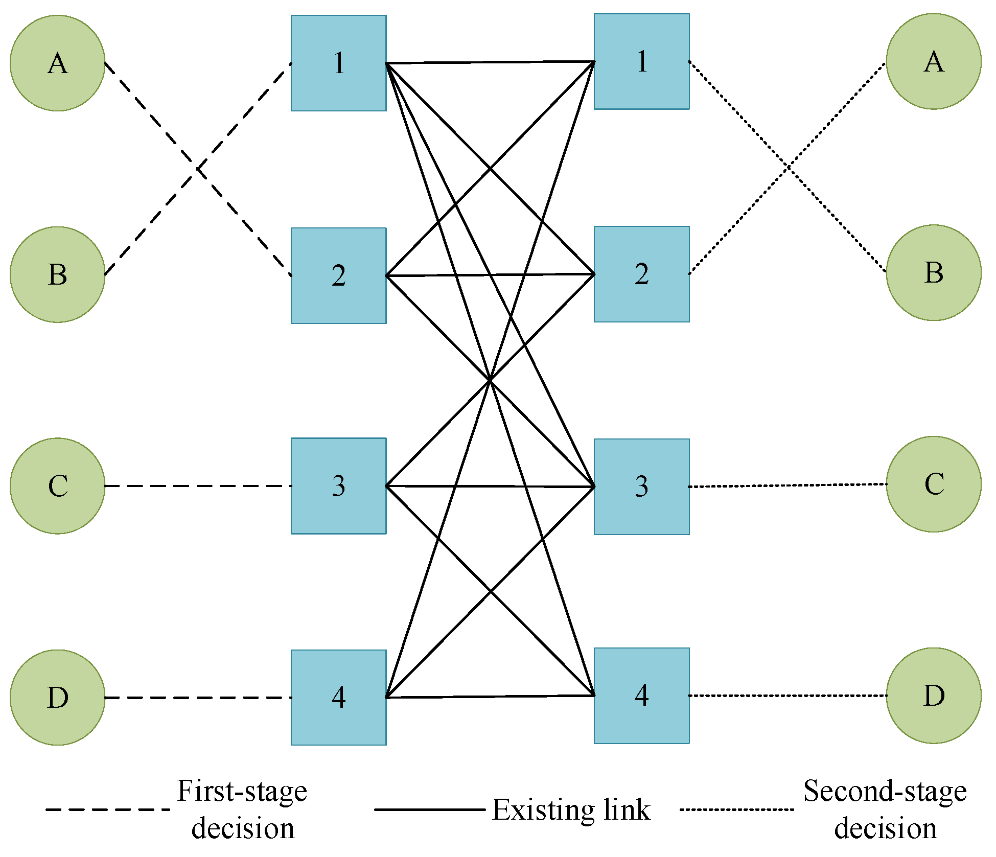
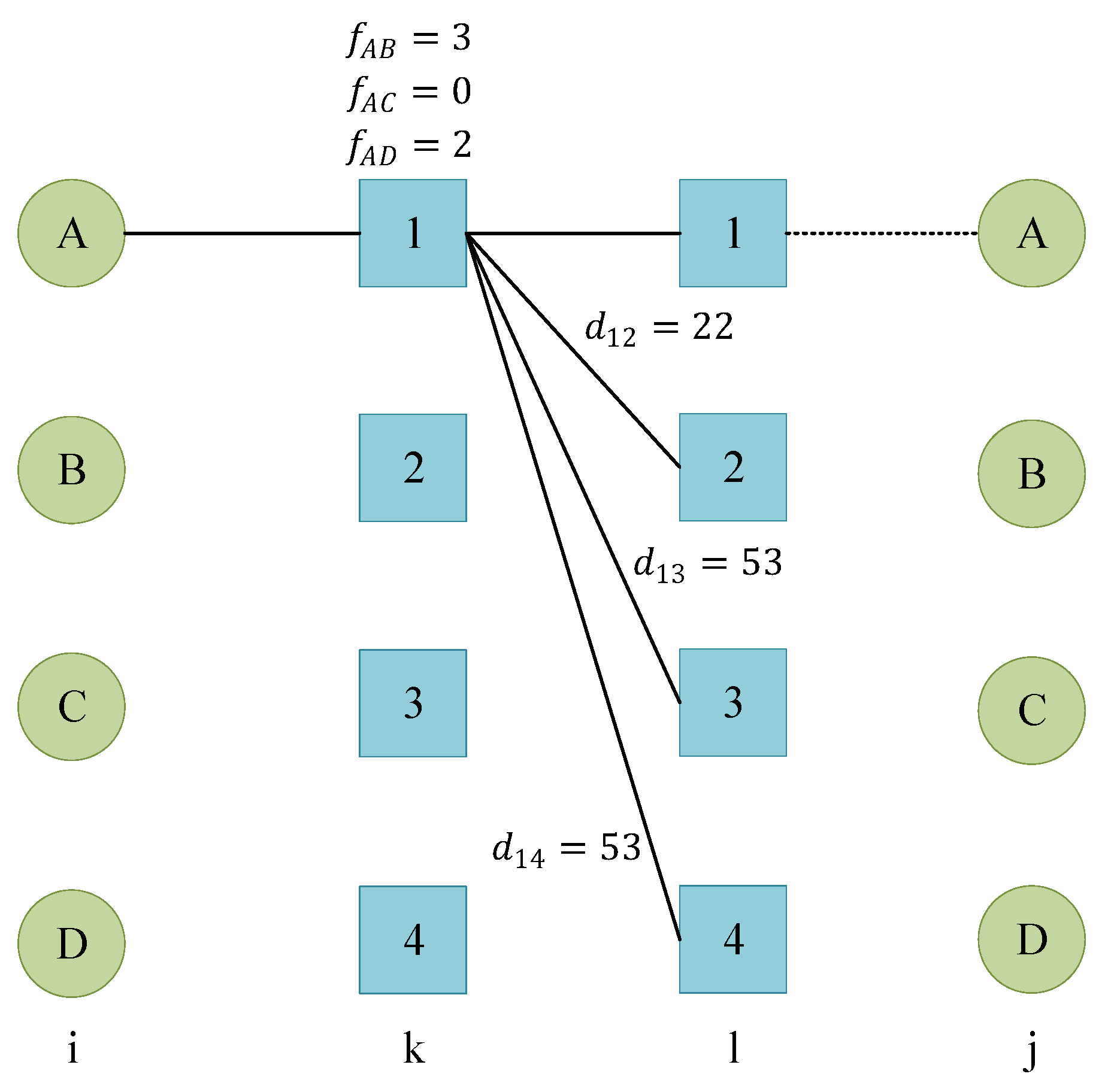
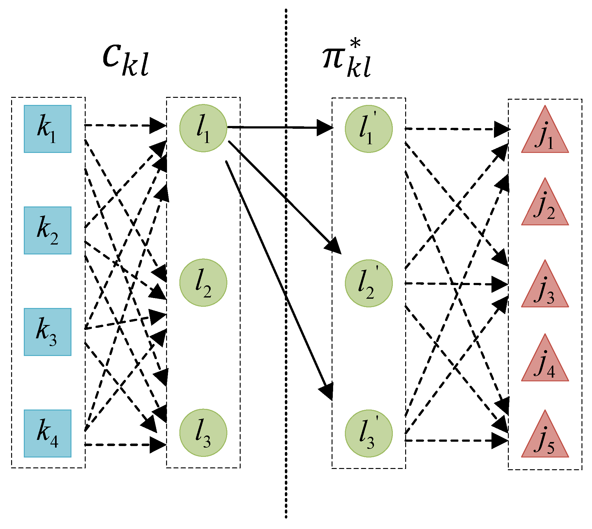
4.1. Stage-Wide Problem Decomposition Schemes of GLB
4.2. Model Decomposition Scheme for Utilizing Efficient Lower Bound Rules for QSAP-C
| Algorithm 1. GLB-based algorithm for obtaining the lower bound of the simplified problem(M2) without enforcing the capacity constraints of DCs. |
| Step 1: Initialization Read the input data, including nodes, links, and agents (flow) Step 2: Calculate the subsequent cost given the decision of |
| For each solve the generalized assignment problem(M3) by calling the Gurobi solver and obtain the value of Step 3: Calculate the estimated cost on the link For each |
| Step 4: Solving the generalized assignment problem by optimizing |
| According to the estimated cost , solve the generalized assignment problem (M4) by calling the Gurobi solver and retrieve the lower bound estimate |
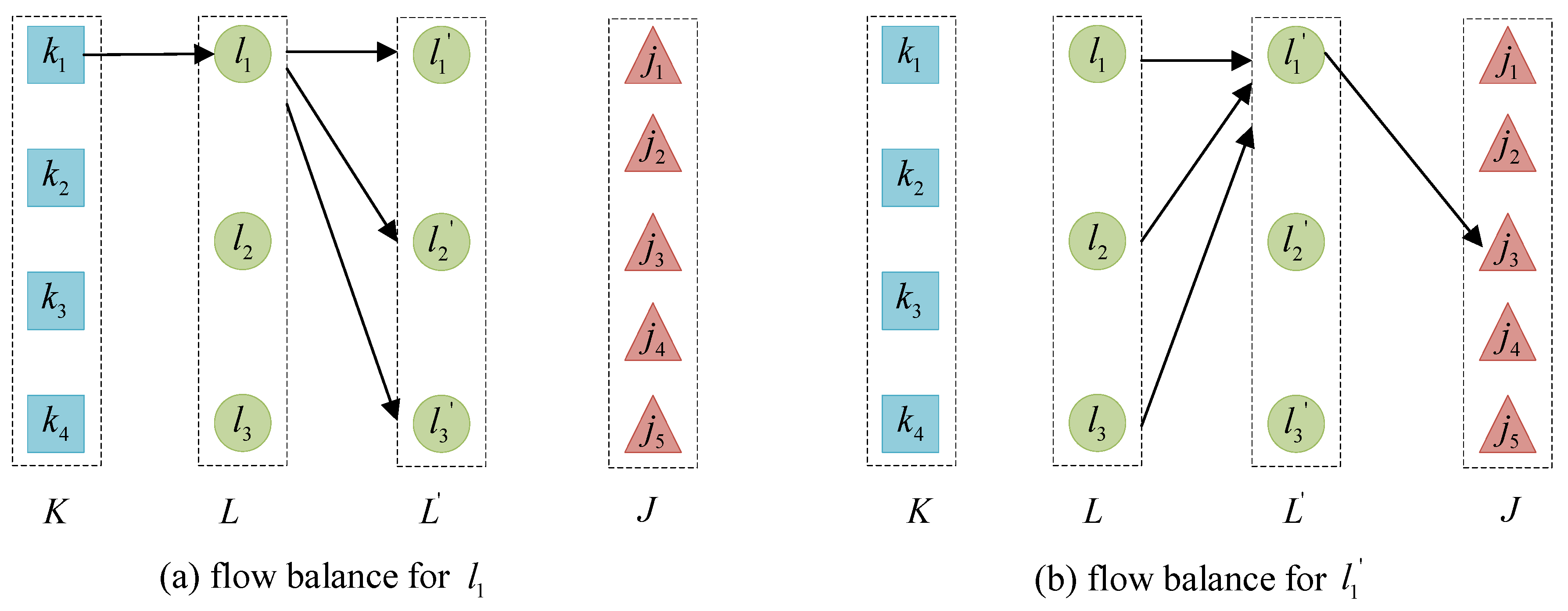
4.3. Connection between Traditional GLB for Standard QAP and Proposed Lower Bound Estimation Process for QSAP-C
4.4. Computation of Upper Bound Solutions
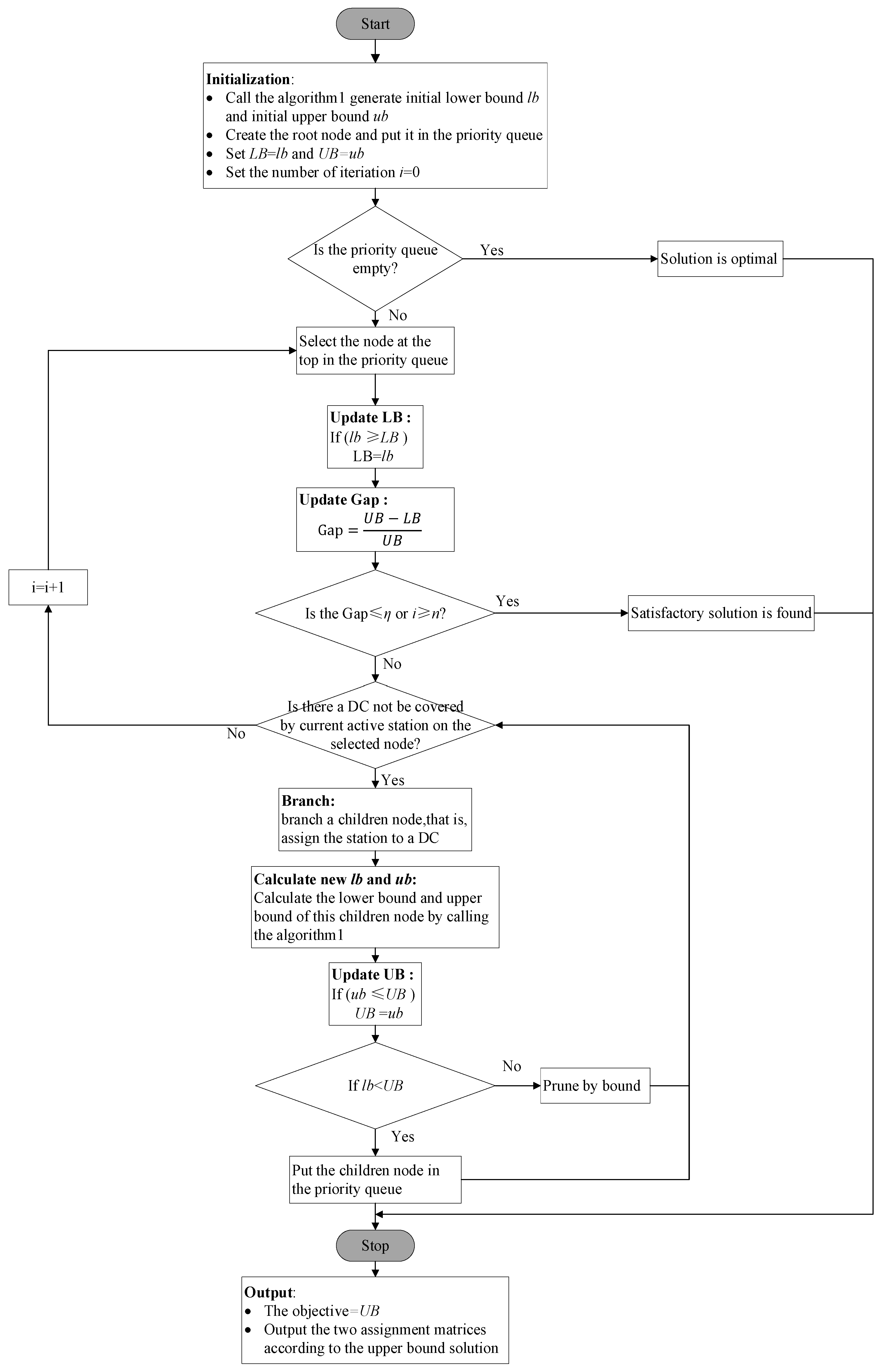
4.5. A Branch-and-Bound Algorithm Combined with Enhanced Lower Bound Rules
| Algorithm 2. A branch-and-bound algorithm combined with heuristic lower bound. |
| Step 1: Initialization Step 1.1: Obtain the initial solution Call Algorithm 1 to obtain the initial lower bound and initial upper bound Set the , Step 1.2: Initialization for the root node and priority queue Create an empty priority queue initialize a root node according to the lower bound, push the root node into the priority queue |
| Step 2: Branch-and-bound process While the is not empty: Step 2.1 Select the top node from the priority queue pq and update the lower bound Pull the top node from the priority queue pq, defined as active_node If active_node.>LB: # update the best global lower bound and the Gap LB = active_node. Gap = If : # check the termination conditions Break If active_node. # update the active station active_node. Else: # all delivery stations have been assigned Continue Step 2.2 Branch on the live node Set temporary matrices # try to assign the to all possible DCs For each DC : Create the children node and inherit the properties of the live node Step 2.3 Calculate the lower bound and upper bound of the children node Call Algorithm 1 to obtain the lower bound and upper bound # update the best global upper bound If children_node.<UB: UB = children_node. If children_node.: Push the children node into the priority queue # otherwise this children node will be pruned |
4.6. An Adaptive Large Neighborhood Search Algorithm with Efficient Initial Solution
| Algorithm 3. An adaptive large neighborhood search algorithm with efficient initial solution. |
| Step 1: Initialization Step 1.1: Obtain the initial solution Call Algorithm 2 to obtain the initial feasible solution in the time limit Step 1.2: Initialization for ALNS Given the total iteration num , initial weight of operators reaction factor |
| Step 2: ALNS For i = 1…Q do select a destroy operator by the roulette-wheel procedure, destroy current solution and obtain the set of removed nodes (2) select a repair operator by the roulette-wheel procedure, repair and obtain the new_solution (3) update the number of times the operator has been used, (4) calculate the objective function of new_solution, if it is infeasible a large constant value will be given. If new_solution_obj <= current_solution_obj update current solution, current_solution_obj = new_solution_obj If current_solution_obj <= best_solution_obj update the best solution, best_solution = current_solution update the success of operators, Else update the success of operators, update the weight of selected operators, If current solution keeps the same for M consecutive iterations break Return the best solution |
4.6.1. Initial Solution
4.6.2. Solution Destruction
- (a)
- Random-remove
- (b) Worst-remove
- (c) Break-remove
- (d) Exchange
4.6.3. Solution Reconstruction
- (a)
- Random-insert
- (b) Greedy-insert
- (c) Regret-insert
4.6.4. Weight Adjustment
5. Numerical Experiments
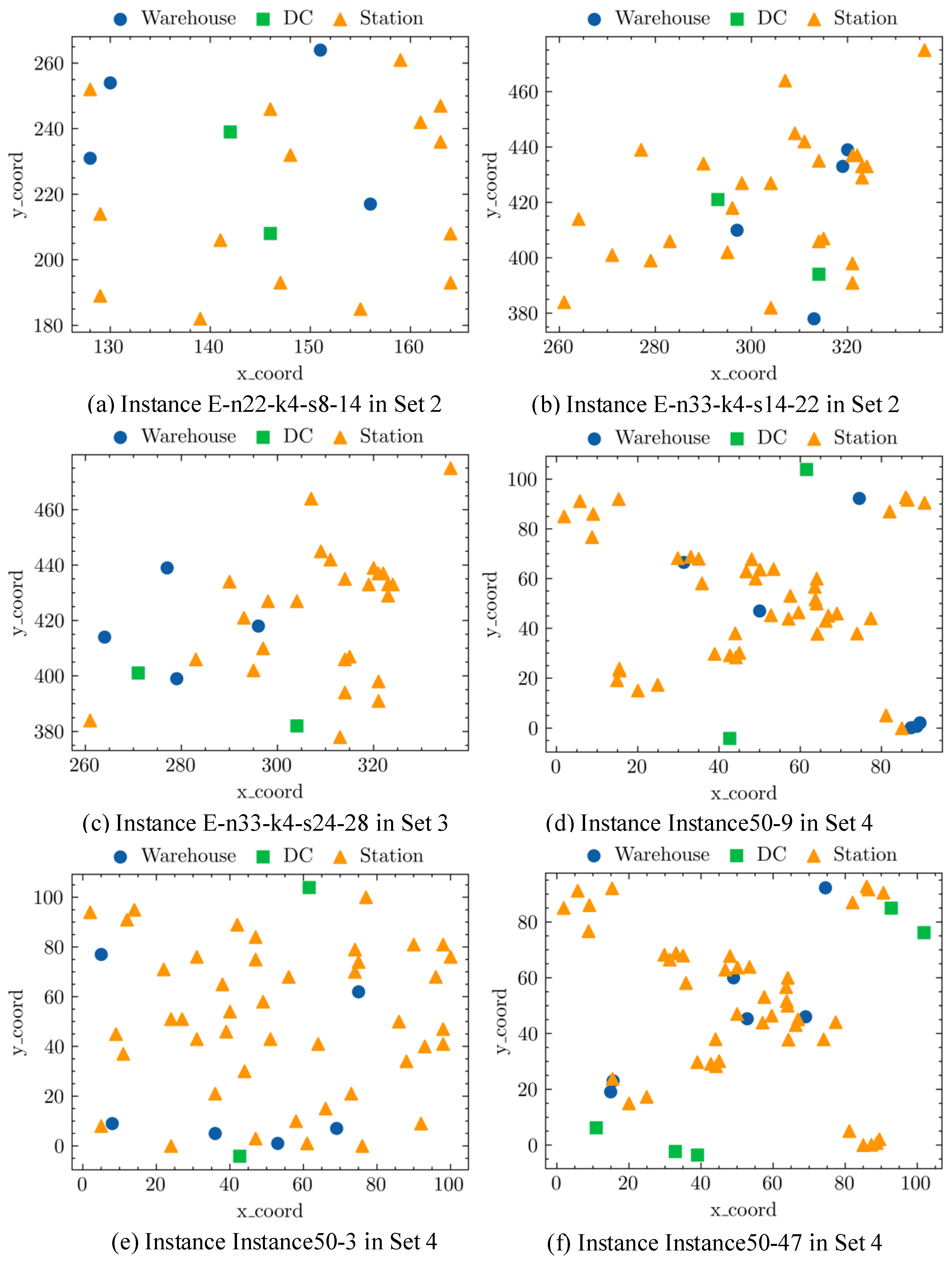
5.1. Base Instance Sets Generation and Description
5.1.1. Locations of Warehouses, DCs, and Delivery Stations
5.1.2. Demand between Warehouses and Delivery Stations
5.1.3. Capacity of DC
5.2. Overall Computational Results
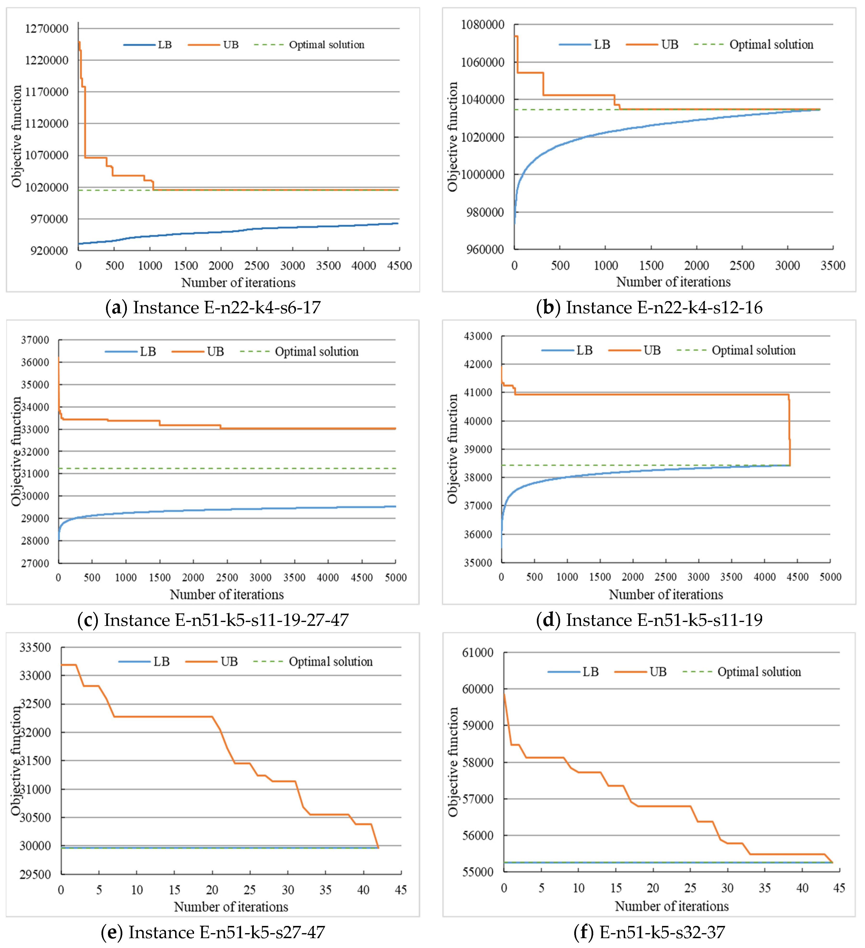
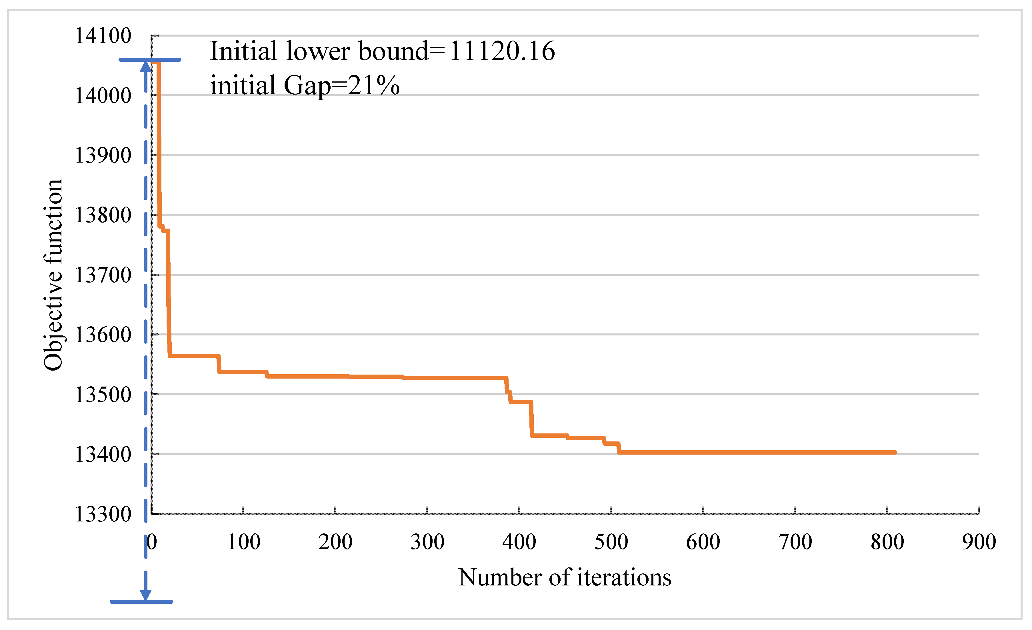
5.3. Convergence and Sensitivity Analysis
5.4. Managerial Insights on Analysis of Algorithms
- (1)
- By adopting the GLB-oriented lower bound, the initial solution with high quality can be obtained efficiently. The average GAP between the initial solution and the optimal solution is within 10%, and the computational time is less than 1 s. The GLB-oriented lower bound estimation process comprehensively considers the cost of the previous decision and the subsequent decision, and the computational time is shortened by decomposing the original problem with quadratic terms in both constraints and objective functions into a series of linear generalized assignment problems. Moreover, this method is sensitive to the locations of different types of nodes, and it is difficult to obtain the initial feasible solution for some instances.
- (2)
- The GLB-oriented lower bound is relatively loose for the original problem. Although the GAP between the initial solution and the optimal solution is usually small, the convergence of branch- and-bound algorithm is slow due to the poor lower bound. For Set 3, the initial solution of several instances has been the optimal solution, and the branch-and-bound process is mainly to improve the lower bound. However, the convergence process analysis shows that the lower bound is not always loose and needs a case-by-case evaluation.
- (3)
- The branch-and-bound algorithm combined with the GLB-oriented lower bound is suitable for solving small-scale examples, while the adaptive large neighborhood search algorithm with efficient initial solution can almost achieve the same effect as the solver. For Set 3, the heuristic algorithm obtains optimal solutions in a relatively short time, and for Set 4, the solution with an average gap of 6% can be obtained within 80% of computational time of the solver. The GLB-oriented lower bound is the main reason to ensure an efficient solution. In some instances, even large neighborhood operations cannot improve the initial solution.
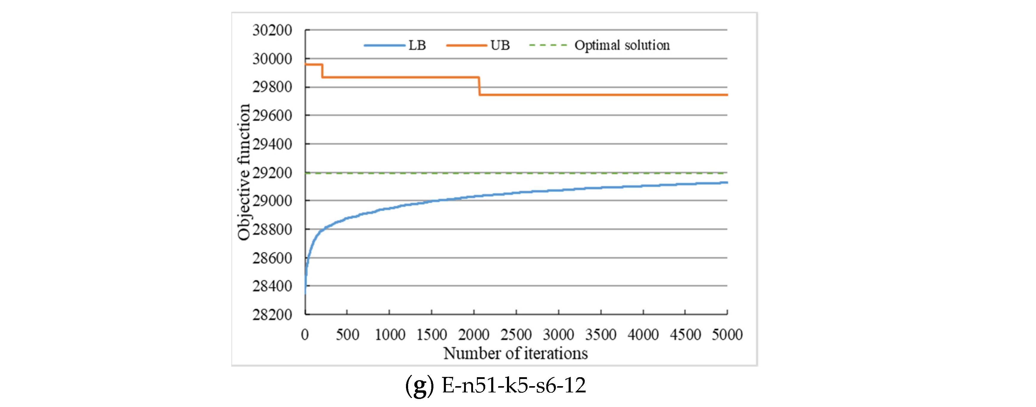
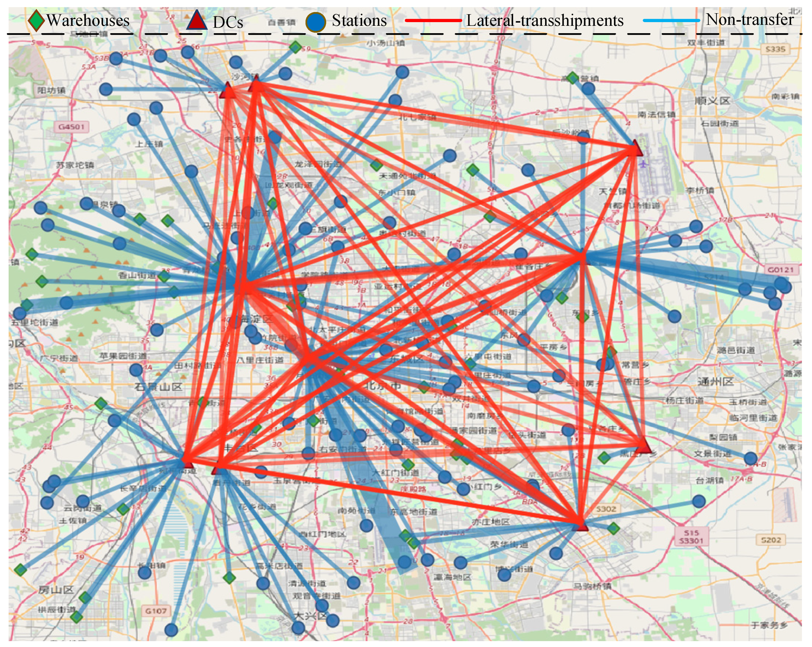
- (4)
- Although lateral-transshipments will make transportation costs higher, it is still the reasonable choice under specific demand pattern. In the sensitive analysis of demand, the proportion of lateral-transshipments volume for some instances up to 70%, and the overall proportion of EP and RP strategies is 40%~50%, which indicates the necessity of lateral-transshipments.
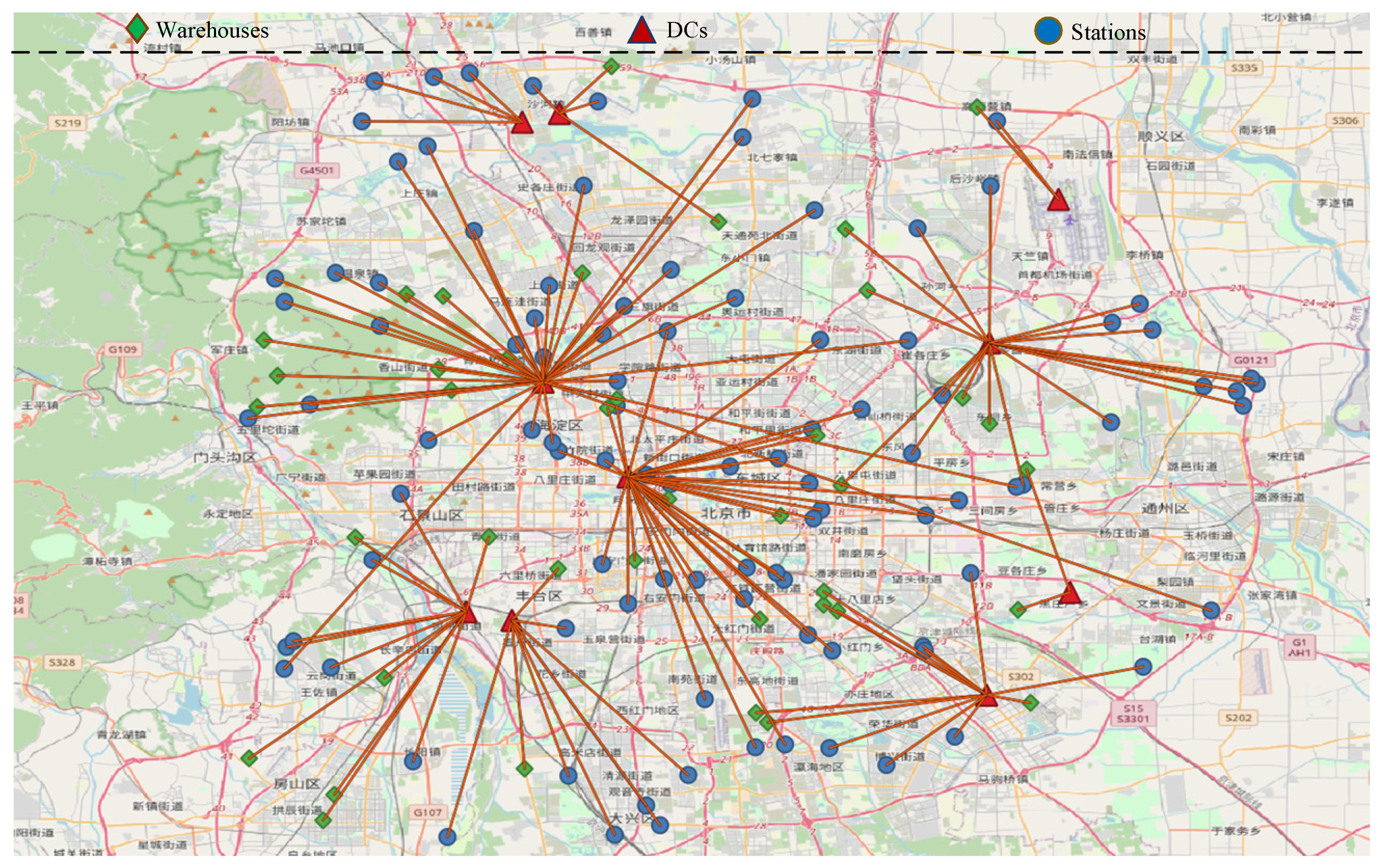
5.5. Real-World Instances
5.6. Managerial Implications for Dynamical Evaluation of Cross-Layer Service Synchronization
5.7. QUBO Formulation of the QSAP-C
6. Conclusions and Future Research
Author Contributions
Funding
Data Availability Statement
Conflicts of Interest
Appendix A
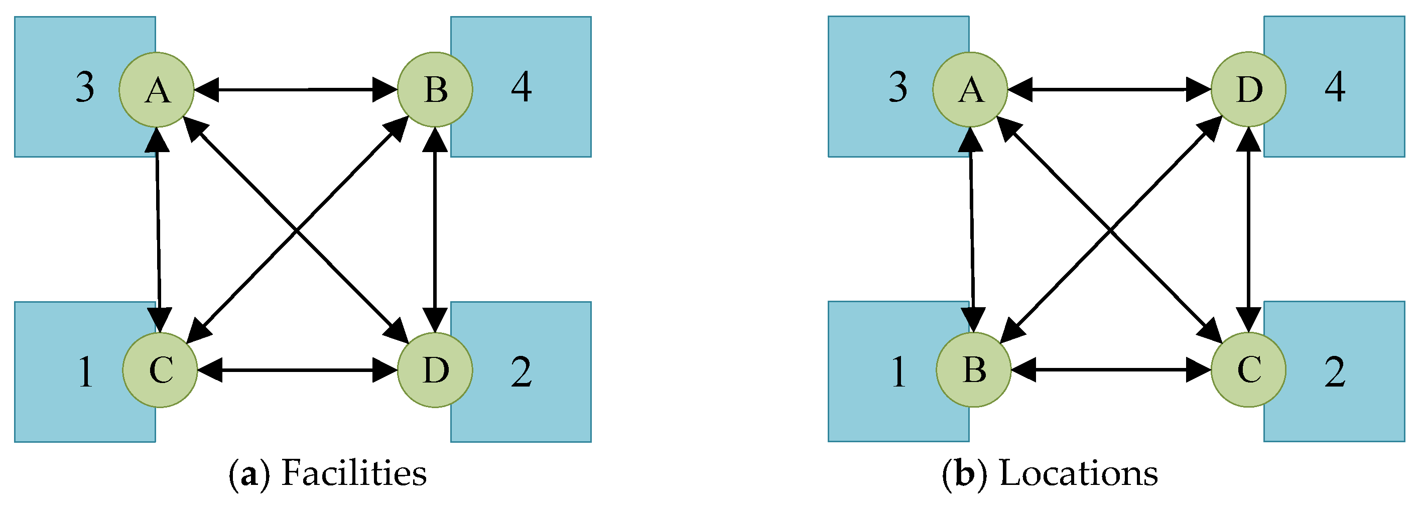
Appendix A.1. The Relationship between Standard QAP and QSAP-C
Appendix A.2. The Quality of Different Lower Bounds

| Instance | GLB62 | RRD95 | HG98 | KCCEB99 | AB01 | RRRP02 | RS03 | R04 | BV04 | HH01 |
|---|---|---|---|---|---|---|---|---|---|---|
| Had16 | 9.7% | - | 4.4% | 4.5% | 3.4% | - | 0.6% | 0 | 1.3% | 0 |
| Had18 | 10.9% | - | 5.1% | 5.2% | 4.0% | - | 0.8% | 0.04% | 1.1% | 0 |
| Had20 | 10.9% | - | 5.1% | 5.1% | 3.5% | - | 0.5% | 0.03% | 1.6% | 0 |
| Kra30a | 23.1% | 14.5% | 14.7% | 15.0% | 22.9% | - | 12.7% | - | 2.5% | 3.0% |
| Kra30b | 24.5% | 16.0% | 16.3% | 16.6% | 24.5% | - | 11.2% | - | 4.1% | 4.7% |
| Nug12 | 14.7% | 9.5% | 9.5% | 9.9% | 13.8% | 0 | 3.6% | 1.9% | 1.7% | 0 |
| Nug15 | 16.3% | 9.5% | 9.7% | 10.2% | 13.0% | - | 2.4% | 1.0% | 0.8% | 0 |
| Nug18 | - | - | - | - | - | - | - | - | - | - |
| Nug20 | 20.0% | 15.1% | 15.2% | 15.4% | 10.9% | - | 4.6% | 3.0% | 2.5% | 2.4% |
| Nug22 | - | - | - | - | - | - | - | - | - | 2.4% |
| Nug30 | 25.9% | 21.5% | 21.7% | 21.9% | 12.4% | - | 5.2% | - | 3.1% | 5.8% |
| Rou15 | 15.7% | 8.3% | 8.5% | 8.6% | 14.2% | - | 5.9% | 1.5% | 1.1% | 0 |
| Rou20 | 22.8% | 11.3% | 11.5% | 11.6% | 16.2% | - | 8.5% | 4.7% | 4.2% | 3.6% |
| Tai20a | 17.5% | - | 12.3% | 12.3% | 16.8% | - | 9.4% | - | 4.5% | 3.9% |
| Tai25a | 17.5% | - | 13.8% | 13.8% | 15.7% | - | 10.8% | - | 4.7% | 6.5% |
| Tai30a | 17.2% | - | 13.9% | 13.9% | 16.5% | - | 9.1% | - | 6.1% | 7.3% |
| Tho30 | 39.6% | 32.8% | 33.3% | 33.4% | 16.8% | - | 9.3% | - | 4.8% | 8.8% |
References
- Ambrosino, D.; Scutella, M.G. Distribution network design: New problems and related models. Eur. J. Oper. Res. 2005, 165, 610–624. [Google Scholar] [CrossRef]
- Puga, M.S.; Minner, S.; Tancrez, J.S. Two-stage supply chain design with safety stock placement decisions. Int. J. Prod. Econ. 2019, 209, 183–193. [Google Scholar] [CrossRef]
- Dehghani, M.; Abbasi, B. An age-based lateral-transshipment policy for perishable items. Int. J. Prod. Econ. 2018, 198, 93–103. [Google Scholar] [CrossRef]
- Paterson, C.; GKiesmüller Teunter, R.; Glazebrook, K. Inventory models with lateral transshipments: A review. Eur. J. Oper. Res. 2011, 210, 125–136. [Google Scholar] [CrossRef]
- Jovan, G. Amiya Chakravarty. Sharing and Lateral Transshipment of Inventory in a Supply Chain with Expensive Low-Demand Items. Manag. Sci. 2001, 47, 579–594. [Google Scholar]
- Rabbani, M.; Sabbaghnia, A.; Mobini, M.; Razmi, J. A graph theory-based algorithm for a multi-echelon multi-period responsive supply chain network design with lateral-transshipments. Oper. Res. 2020, 20, 2497–2517. [Google Scholar] [CrossRef]
- Domschke, W. Schedule synchronization for public transit networks. Oper.-Res.-Spektrum 1989, 11, 17–24. [Google Scholar] [CrossRef]
- Hahn, P.M.; Kim, B.J.; Guignard, M.; Smith, J.M.; Zhu, Y.R. An algorithm for the generalized quadratic assignment problem. Comput. Optim. Appl. 2008, 40, 351–372. [Google Scholar] [CrossRef]
- Bertsimas, D.; Delarue, A.; Martin, S. Optimizing schools’ start time and bus routes. Proc. Natl. Acad. Sci. USA 2019, 116, 5943–5948. [Google Scholar] [CrossRef]
- Glover, F.; Lewis, M.; Kochenberger, G. Logical and inequality implications for reducing the size and difficulty of quadratic unconstrained binary optimization problems. Eur. J. Oper. Res. 2018, 265, 829–842. [Google Scholar] [CrossRef]
- Glover, F.; Kochenberger, G.; Hennig, R.; Du, Y. Quantum Bridge Analytics I: A tutorial on formulating and using QUBO models. Ann. Oper. Res. 2022, 314, 141–183. [Google Scholar] [CrossRef]
- Kochenberger, G.A.; Glover, F. A unified framework for modeling and solving combinatorial optimization problems: A tutorial. In Multiscale Optimization Methods and Applications; Springer: Boston, MA, USA, 2006; pp. 101–124. [Google Scholar]
- Zhang, H.; Liu, F.; Zhou, Y.; Zhang, Z. A hybrid method integrating an elite genetic algorithm with tabu search for the quadratic assignment problem. Inf. Sci. 2020, 539, 347–374. [Google Scholar] [CrossRef]
- Dokeroglu, T.; Sevinc, E.; Cosar, A. Artificial bee colony optimization for the quadratic assignment problem. Appl. Soft Comput. 2019, 76, 595–606. [Google Scholar] [CrossRef]
- Peng, Z.Y.; Huang, Y.J.; Zhong, Y.B. A discrete artificial bee colony algorithm for quadratic assignment problem. J. High Speed Netw. 2022, 28, 131–141. [Google Scholar] [CrossRef]
- Wang, H.; Alidaee, B. A New Hybrid-heuristic for Large-scale Combinatorial Optimization: A Case of Quadratic Assignment Problem. Comput. Ind. Eng. 2023, 179, 109220. [Google Scholar] [CrossRef]
- Shahabi, M.; Akbarinasaji, S.; Unnikrishnan, A.; James, R. Integrated inventory control and facility location decisions in a multi-echelon supply chain network with hubs. Netw. Spat. Econ. 2013, 13, 497–514. [Google Scholar] [CrossRef]
- Shi, J.; Zhang, G.; Sha, J. A Lagrangian based solution algorithm for a build-to-order supply chain network design problem. Adv. Eng. Softw. 2012, 49, 21–28. [Google Scholar] [CrossRef]
- Jang, Y.J.; Jang, S.Y.; Chang, B.M.; Park, J. A combined model of network design and production/distribution planning for a supply network. Comput. Ind. Eng. 2002, 43, 263–281. [Google Scholar] [CrossRef]
- Manupati, V.K.; Jedidah, S.J.; Gupta, S.; Bhandari, A.; Ramkumar, M. Optimization of a multi-echelon sustainable production-distribution supply chain system with lead time consideration under carbon emission policies. Comput. Ind. Eng. 2019, 135, 1312–1323. [Google Scholar] [CrossRef]
- Melo, M.T.; Nickel, S.; Saldanha-Da-Gama, F. Facility location and supply chain management–A review. Eur. J. Oper. Res. 2009, 196, 401–412. [Google Scholar] [CrossRef]
- Devika, K.; Jafarian, A.; Nourbakhsh, V. Designing a sustainable closed-loop supply chain network based on triple bottom line approach: A comparison of metaheuristics hybridization techniques. Eur. J. Oper. Res. 2014, 235, 594–615. [Google Scholar] [CrossRef]
- Eskandarpour, M.; Dejax, P.; Miemczyk, J.; Péton, O. Sustainable supply chain network design: An optimization-oriented review. Omega 2015, 54, 11–32. [Google Scholar] [CrossRef]
- Wang, H.S. A two-phase ant colony algorithm for multi-echelon defective supply chain network design. Eur. J. Oper. Res. 2009, 192, 243–252. [Google Scholar] [CrossRef]
- Wang, K.J.; Makond, B.; Liu, S.Y. Location and allocation decisions in a two-echelon supply chain with stochastic demand–A genetic-algorithm based solution. Expert Syst. Appl. 2011, 38, 6125–6131. [Google Scholar] [CrossRef]
- Park, S.; Lee, T.E.; Sung, C.S. A three-level supply chain network design model with risk-pooling and lead times. Transp. Res. Part E Logist. Transp. Rev. 2010, 46, 563–581. [Google Scholar] [CrossRef]
- Mogale, D.G.; Kumar, M.; Kumar, S.K.; Tiwari, M.K. Grain silo location-allocation problem with dwell time for optimization of food grain supply chain network. Transp. Res. Part E Logist. Transp. Rev. 2018, 111, 40–69. [Google Scholar] [CrossRef]
- Barbarosoğlu, G.; Özgür, D. Hierarchical design of an integrated production and 2-echelon distribution system. Eur. J. Oper. Res. 1999, 118, 464–484. [Google Scholar] [CrossRef]
- Chen, P.; Pinto, J.M. Lagrangean-based techniques for the supply chain management of flexible process networks. Comput. Chem. Eng. 2008, 32, 2505–2528. [Google Scholar] [CrossRef]
- Farahani, R.Z.; Elahipanah, M. A genetic algorithm to optimize the total cost and service level for just-in-time distribution in a supply chain. Int. J. Prod. Econ. 2008, 111, 229–243. [Google Scholar] [CrossRef]
- Park, Y.B. An integrated approach for production and distribution planning in supply chain management. Int. J. Prod. Res. 2005, 43, 1205–1224. [Google Scholar] [CrossRef]
- Tsiakis, P.; Papageorgiou, L.G. Optimal production allocation and distribution supply chain networks. Int. J. Prod. Econ. 2008, 111, 468–483. [Google Scholar] [CrossRef]
- Akbari, A.A.; Karimi, B. A new robust optimization approach for integrated multi-echelon, multi-product, multi-period supply chain network design under process uncertainty. Int. J. Adv. Manuf. Technol. 2015, 79, 229–244. [Google Scholar] [CrossRef]
- Fard AM, F.; Hajiaghaei-Keshteli, M. A bi-objective partial interdiction problem considering different defensive systems with capacity expansion of facilities under imminent attacks. Appl. Soft Comput. 2018, 68, 343–359. [Google Scholar] [CrossRef]
- Fard AM, F.; Hajaghaei-Keshteli, M. A tri-level location-allocation model for forward/reverse supply chain. Appl. Soft Comput. 2018, 62, 328–346. [Google Scholar] [CrossRef]
- Badri, H.; Ghomi, S.F.; Hejazi, T.H. A two-stage stochastic programming approach for value-based closed-loop supply chain network design. Transp. Res. Part E Logist. Transp. Rev. 2017, 105, 1–17. [Google Scholar] [CrossRef]
- Fattahi, M.; Govindan, K.; Keyvanshokooh, E. Responsive and resilient supply chain network design under operational and disruption risks with delivery lead-time sensitive customers. Transp. Res. Part E Logist. Transp. Rev. 2017, 101, 176–200. [Google Scholar] [CrossRef]
- Aikens, C.H. Facility location models for distribution planning. Eur. J. Oper. Res. 1985, 22, 263–279. [Google Scholar] [CrossRef]
- Vidal, C.J.; Goetschalckx, M. Strategic production-distribution models: A critical review with emphasis on global supply chain models. Eur. J. Oper. Res. 1997, 98, 1–18. [Google Scholar] [CrossRef]
- Fahimnia, B.; Farahani, R.Z.; Marian, R.; Luong, L. A review and critique on integrated production–distribution planning models and techniques. J. Manuf. Syst. 2013, 32, 1–19. [Google Scholar] [CrossRef]
- Goetschalckx, M.; Vidal, C.J.; Dogan, K. Modeling and design of global logistics systems: A review of integrated strategic and tactical models and design algorithms. Eur. J. Oper. Res. 2002, 143, 1–18. [Google Scholar] [CrossRef]
- Chen, Z.L. Integrated production and outbound distribution scheduling: Review and extensions. Oper. Res. 2010, 58, 130–148. [Google Scholar] [CrossRef]
- Fisher, M.L.; Jörnsten, K.O.; Madsen, O.B. Vehicle routing with time windows: Two optimization algorithms. Oper. Res. 1997, 45, 488–492. [Google Scholar] [CrossRef]
- Shen ZJ, M.; Coullard, C.; Daskin, M.S. A joint location-inventory model. Transp. Sci. 2003, 37, 40–55. [Google Scholar] [CrossRef]
- Pan, F.; Nagi, R. Multi-echelon supply chain network design in agile manufacturing. Omega 2013, 41, 969–983. [Google Scholar] [CrossRef]
- Ben Abid, T.; Ayadi, O.; Masmoudi, F. An integrated production-distribution planning problem under demand and production capacity uncertainties: New formulation and case study. Math. Probl. Eng. 2020, 2020, 1520764. [Google Scholar] [CrossRef]
- Larimi, N.G.; Yaghoubi, S.; Hosseini-Motlagh, S.M. Itemized platelet supply chain with lateral transshipment under uncertainty evaluating inappropriate output in laboratories. Socio-Econ. Plan. Sci. 2019, 68, 100697. [Google Scholar] [CrossRef]
- Tsiakis, P.; Shah, N.; Pantelides, C.C. Design of multi-echelon supply chain networks under demand uncertainty. Ind. Eng. Chem. Res. 2001, 40, 3585–3604. [Google Scholar] [CrossRef]
- Finke, G.; Burkard, R.E.; Rendl, F. Quadratic assignment problems. North-Holl. Math. Stud. 1987, 132, 61–82. [Google Scholar]
- Abdel-Basset, M.; Manogaran, G.; Rashad, H.; Zaied, A.N.H. A comprehensive review of quadratic assignment problem: Variants, hybrids and applications. J. Ambient. Intell. Humaniz. Comput. 2018, 1–24. [Google Scholar] [CrossRef]
- Burkard, R.E.; Cela, E.; Pardalos, P.M.; Pitsoulis, L.S. The quadratic assignment problem. In Handbook of Combinatorial Optimization; Springer: Boston, MA, USA, 1998; pp. 1713–1809. [Google Scholar]
- Burkard, R.; Dell’Amico, M.; Martello, S. Assignment Problems: Revised Reprint; Society for Industrial and Applied Mathematics: Philadelphia, PA, USA, 2012. [Google Scholar]
- Li, Y.; Pardalos, P.M.; Ramakrishnan, K.G.; Resende, M.G. Lower bounds for the quadratic assignment problem. Ann. Oper. Res. 1994, 50, 387–410. [Google Scholar] [CrossRef]
- Pisinger, D.; Ropke, S. A general heuristic for vehicle routing problems. Comput. Oper. Res. 2007, 34, 2403–2435. [Google Scholar] [CrossRef]
- Lutz, R. Adaptive Large Neighborhood Search. Bachelor’s Thesis, Ulm University, Ulm, Germany, 2015. [Google Scholar]
- Yu, C.; Zhang, D.; Lau, H.Y. An adaptive large neighborhood search heuristic for solving a robust gate assignment problem. Expert Syst. Appl. 2017, 84, 143–154. [Google Scholar] [CrossRef]
- Perboli, G.; Tadei, R.; Vigo, D. The two-echelon capacitated vehicle routing problem: Models and math-based heuristics. Transp. Sci. 2011, 45, 364–380. [Google Scholar] [CrossRef]
- Crainic, T.G.; Perboli, G.; Mancini, S.; Tadei, R. Two-echelon vehicle routing problem: A satellite location analysis. Procedia-Soc. Behav. Sci. 2010, 2, 5944–5955. [Google Scholar] [CrossRef]
- Wu, X.B.; Lu, J.; Wu, S.; Zhou, X.S. Synchronizing time-dependent transportation services: Reformulation and solution algorithm using quadratic assignment problem. Transp. Res. Part B Methodol. 2021, 152, 140–179. [Google Scholar] [CrossRef]
- Ayodele, M.; Allmendinger, R.; López-Ibáñez, M.; Parizy, M. Multi-objective QUBO solver: Bi-objective quadratic assignment problem. In Proceedings of the Genetic and Evolutionary Computation Conference, Boston, MA, USA, 9–13 June 2022. [Google Scholar]
- Verma, A.; Lewis, M. Penalty and partitioning techniques to improve performance of QUBO solvers. Discret. Optim. 2020, 44, 100594. [Google Scholar] [CrossRef]
- Mayowa, A. Penalty Weights in QUBO Formulations: Permutation Problems. In Proceedings of the EvoCOP 2022–22nd European Conference on Evolutionary Computation in Combinatorial Optimization, Madrid, Spain, 20–22 April 2022; Leslie, P.C., Sébastien, V., Eds.; Springer: Cham, Switzerland, 2022; pp. 159–174. [Google Scholar]
- Lu, J.; Nie, Q.; Mahmoudi, M.; Ou, J.; Li, C.; Zhou, X.S. Rich arc routing problem in city logistics: Models and solution algorithms using a fluid queue-based time-dependent travel time representation. Transp. Res. Part B Methodol. 2022, 166, 143–182. [Google Scholar] [CrossRef]
- Gilmore, P.C. Optimal and suboptimal algorithms for the quadratic assignment problem. J. Soc. Ind. Appl. Math. 1962, 10, 305–313. [Google Scholar] [CrossRef]
- Resende, M.G.; Ramakrishnan, K.G.; Drezner, Z. Computing lower bounds for the quadratic assignment problem with an interior point algorithm for linear programming. Oper. Res. 1995, 43, 781–791. [Google Scholar] [CrossRef]
- Hahn, P.; Grant, T. Lower bounds for the quadratic assignment problem based upon a dual formulation. Oper. Res. 1998, 46, 912–922. [Google Scholar] [CrossRef]
- Karisch, S.E.; Cela, E.; Clausen, J.; Espersen, T. A dual framework for lower bounds of the quadratic assignment problem based on linearization. Computing 1999, 63, 351–403. [Google Scholar] [CrossRef]
- Anstreicher, K.M.; Brixius, N.W. A new bound for the quadratic assignment problem based on convex quadratic programming. Math. Program. 2001, 89, 341–357. [Google Scholar] [CrossRef]
- Ramakrishnan, K.G.; Resende MG, C.; Ramachandran, B.; Pekny, J.F. Tight QAP bounds via linear programming. In Combinatorial and Global Optimization; World Scientific: Singapore, 2002; pp. 297–303. [Google Scholar]
- Sotirov, R.; Rendl, F. Bounds for the quadratic assignment problem using the bundle method. In Discrete Optimization: Methods and Applications; University of Klagenfurt: Klagenfurt, Austria, 2003; pp. 287–305. [Google Scholar]
- Roupin, F. From linear to semidefinite programming: An algorithm to obtain semidefinite relaxations for bivalent quadratic problems. J. Comb. Optim. 2004, 8, 469–493. [Google Scholar] [CrossRef]
- Burer, S.; Vandenbussche, D. Solving lift-and-project relaxations of binary integer programs. SIAM J. Optim. 2006, 16, 726–750. [Google Scholar] [CrossRef]
- Adams, W.P.; Guignard, M.; Hahn, P.M.; Hightower, W.L. A level-2 reformulation–linearization technique bound for the quadratic assignment problem. Eur. J. Oper. Res. 2007, 180, 983–996. [Google Scholar] [CrossRef]


| Publication | Number of Echelons | Model | Problem Decomposition Schemes | Solution Algorithms |
|---|---|---|---|---|
| [28] | 2 | MIP, linear | Lagrangian relaxation | LR |
| [19] | 7 | MIP, linear | Sequential; Lagrangian relaxation | LR; GA |
| [31] | 2 | MIP, linear | Two-phase heuristic | LS |
| [30] | 3 | MIP, linear | - | GA |
| [32] | 3 | MIP, linear | - | CPLEX solver |
| [18] | 3 | 0–1 IP, linear | Lagrangian relaxation | LR |
| [17] | 4 | CQMIP, nonlinear | - | CPLEX solver |
| [22] | 9 | MIP, linear | - | AICA; VNS |
| [33] | 3 | MIP, linear | - | CPLEX solver; Simulation |
| [35] | 4 | MIP, nonlinear | Nested approach | VNS; TS; PSO; KA; WWO |
| [20] | 3 | MIP, nonlinear | Sequential | Heuristic |
| [6] | 4 | MIP, linear | Sequential | Heuristic; GAMS |
| This paper | 3 | 0–1 IP, nonlinear | Two-stage decomposition via cost estimation | BB; ALNS |
| Publication | Network Planning Strategy | Decomposition/Linearization Method | Cost Propagation | Illustration of Key Decision Variables |
|---|---|---|---|---|
| [17] | single sourcing, lateral-transshipments and direct shipment are prohibited | by introducing a new binary variable to linearize the binary quadratic terms in the objective function, then solve it using the CPLEX 12 solver | - |  |
| [6] | multiple sourcing, lateral-transshipments and direct shipment are allowed | convert the supply chain network to a bipartite graph and divide the problem into three main sub-problems: plant-DCs (), DCs-retailers (), and retailers-customers ( | solve three sub-problems sequentially (), the cost of each edge is calculated with respect to the two different end of it and it propagates forward |  |
| This paper | single sourcing, lateral-transshipments are allowed and direct shipments are prohibited | reconstruct the network relationships within DC echelons from the classical quadratic assignment modeling and divide the problem into two stage sub-problems: warehouses-DCs () and DCs-retailers () | for each fixed , solve sub-problems of DCs-retailers (); solve sub-problems of warehouses-DCs based the solution of DCs-retailers () It has both forward calculation and cost backward propagation |  |
| Symbol | Definition |
|---|---|
| Sets | |
| Set of nodes in the physical network | |
| E | Set of transportation links in the physical network |
| Set of transportation links to be built in the physical network, | |
| Set of transportation links existing in the physical network, | |
| Set of warehouses, | |
| Set of DCs, | |
| Set of stations, | |
| Indices | |
| Index of set , | |
| Index of set , | |
| Index of the set , | |
| Index of set , | |
| Parameters | |
| Distance from warehouse to DC | |
| Estimated cost from warehouse to DC | |
| Distance from DC to DC | |
| Distance from DC to station | |
| Demand for station at warehouse | |
| Capacity of the DC |
| =1 if assign warehouse k to distribution center , = 0 otherwise | |
| =1 if assign station to the distribution center , = 0 otherwise |
| Elements | Original Network | Extended Network | Distance |
|---|---|---|---|
| node | |||
| node | |||
| link | |||
| link | |||
| path | |||
| path |
| Step | Formula | Illustration |
|---|---|---|
| Estimate the second-stage cost by fixing the decision variable in the first stage | Let , the optimal solution of following linear assignment problem is defined as for each |  |
| Calculate the total cost for each as BCE | - | |
| Solve the first-stage problem based on BCE of |  |
| 1 | 2 | 3 | 4 | |
|---|---|---|---|---|
| 1 | 0 | 22 | 53 | 53 |
| 2 | 22 | 0 | 40 | 62 |
| 3 | 53 | 40 | 0 | 55 |
| 4 | 53 | 62 | 55 | 0 |
| A | B | C | D | |
|---|---|---|---|---|
| A | 0 | 3 | 0 | 2 |
| B | 3 | 0 | 0 | 1 |
| C | 0 | 0 | 0 | 4 |
| D | 2 | 1 | 4 | 0 |
| 1 | 2 | 3 | 4 | |
|---|---|---|---|---|
| A | ||||
| B | ||||
| C | 226 | |||
| D | 212 | 0 |
| GLB for Standard QAP | Lower Bound Estimation in QSAP-C | ||
|---|---|---|---|
| First stage decision | problem type | LAPs | GLAPs |
| cost | fixed cost independent of flows | the product of distances and flows | |
| Second stage decision | problem type | LAPs | GLAPs |
| cost | fixed cost independent of flows | the product of distances and flows | |
| Cost backward propagation | Optimal solutions of the LAPs in second stage decision | Optimal solutions of the GLAPs in second stage decision | |
| Set | Number of Instances | Number of Warehouses | Number of DCs | Number of Stations | Capacity of Each DC |
|---|---|---|---|---|---|
| 2 | 6 | 4 | 2 | 15 | 12,000 |
| 2 | 6 | 4 | 2 | 26 | 16,000 |
| 2 | 3 | 4 | 4 | 42 | 500 |
| 2 | 6 | 4 | 2 | 44 | 1000 |
| 3 | 6 | 4 | 2 | 15 | 12,000 |
| 3 | 6 | 4 | 2 | 26 | 16,000 |
| 3 | 6 | 4 | 2 | 44 | 1000 |
| 4 | 18 | 6 | 2 | 44 | 15,000 |
| 4 | 18 | 6 | 3 | 44 | 20,000 |
| 4 | 18 | 6 | 5 | 44 | 24,000 |
| Gurobi | BB | ALNS | ||||||||||
|---|---|---|---|---|---|---|---|---|---|---|---|---|
| Instance | Warehouses ID | OPT | T_G (s) | BEST_SOL1 | GAP1 | T_B (s) | INIT_SOL | GAP2 | T_B_I (s) | BEST_SOL2 | GAP3 | T_A (s) |
| Set 2 | ||||||||||||
| E-n22-k4-s10-14 | 3, 11, 13, 20 | - | 0.44 | - | - | 142.24 | - | - | 1.07 | - | - | 1.95 |
| E-n22-k4-s11-12 | 2, 8, 15, 17 | - | 0.27 | - | - | 141.90 | - | - | 0.02 | - | - | 1.91 |
| E-n22-k4-s12-16 | 2, 4, 9, 17 | 1,034,673.25 | 0.17 | 1,034,673.25 | 0 | 97.48 | 1,073,847.25 | 0.04 | 0.36 | 1,034,673.25 | 0 | 1.14 |
| E-n22-k4-s6-17 | 7, 16, 19, 21 | 1,015,276.50 | 0.31 | 1,015,276.5 | 0 | 168.92 | 1,248,893.50 | 0.23 | 33.21 | 1,015,276.50 | 0 | 2.06 |
| E-n22-k4-s8-14 | 1, 3, 11, 12 | - | 0.28 | - | - | 144.06 | - | - | 0.02 | - | - | 1.92 |
| E-n22-k4-s9-19 | 2, 8, 13, 15 | - | 0.28 | - | - | 139.90 | - | - | 0.02 | - | - | 1.97 |
| E-n33-k4-s1-9 | 3, 5, 18, 19 | - | 0.30 | - | - | 281.21 | - | - | 0.02 | - | - | 2.5 |
| E-n33-k4-s14-22 | 5, 17, 23, 32 | - | 0.34 | - | - | 261.08 | - | - | 0.03 | - | - | 2.52 |
| E-n33-k4-s2-13 | 8, 12, 19, 21 | - | 0.41 | - | - | 260.54 | - | - | 0.03 | - | - | 2.48 |
| E-n33-k4-s3-17 | 14, 20, 25, 27 | - | 0.42 | - | - | 318.96 | - | - | 0.05 | - | - | 2.66 |
| E-n33-k4-s4-5 | 13, 15, 27, 31 | - | 0.42 | - | - | 304.99 | - | - | 0.03 | - | - | 2.5 |
| E-n33-k4-s7-25 | 5, 11, 12, 20 | - | 0.27 | - | - | 260.56 | - | - | 0.03 | - | - | 2.41 |
| E-n51-k5-s11-19-27-47 | 20, 26, 35, 49 | 31,225.74 | 8.86 | 33,026.46 | 0.06 | 2772.59 | 36,200.85 | 0.16 | 0.17 | 35,362.62 | 0.13 | 9.86 |
| E-n51-k5-s11-19 | 2, 13, 23, 46 | 38,424.49 | 0.16 | 38,424.49 | 0 | 374.50 | 41,906.84 | 0.09 | 0.11 | 39,643.09 | 0.03 | 3.26 |
| E-n51-k5-s2-17 | 5, 12, 15, 42 | 38,123.45 | 0.16 | 38,123.45 | 0 | 3.71 | 40,924.43 | 0.07 | 0.06 | 38,158.67 | 0 | 3.16 |
| E-n51-k5-s2-4-17-46 | 3, 5, 32, 33 | 32,179.54 | 2.00 | 34,922.4 | 0.09 | 2481.72 | 35,839.62 | 0.11 | 0.13 | 35,278.47 | 0.1 | 13.88 |
| E-n51-k5-s27-47 | 5, 31, 42, 48 | 29,960.37 | 0.14 | 29,960.37 | 0 | 3.46 | 33,184.19 | 0.11 | 0.09 | 30,060.14 | 0 | 3.1 |
| E-n51-k5-s32-37 | 15, 16, 18, 30 | 55,265.48 | 0.14 | 55,265.48 | 0 | 4.04 | 59,857.78 | 0.08 | 0.05 | 55,571.24 | 0.01 | 3.94 |
| E-n51-k5-s4-46 | 17, 23, 34, 47 | 45,900.66 | 0.16 | 49,731.34 | 0.08 | 425.31 | 50,887.61 | 0.11 | 0.04 | 46,930.39 | 0.02 | 2.52 |
| E-n51-k5-s6-12-32-37 | 9, 20, 27, 35 | 35,067.50 | 1.78 | 36,834.41 | 0.05 | 2771.15 | 37,583.28 | 0.07 | 0.16 | 36,850.91 | 0.05 | 8.93 |
| E-n51-k5-s6-12 | 3, 15, 21, 48 | 29,194.02 | 0.19 | 29,744.63 | 0.02 | 425.92 | 29,962.32 | 0.03 | 0.11 | 29,918.82 | 0.02 | 2.41 |
| Average | 0.83 | 0.02 | 561.15 | 0.1 | 1.71/0.55 | 0.03 | 3.67 | |||||
| Gurobi | BB | ALNS | ||||||||||
|---|---|---|---|---|---|---|---|---|---|---|---|---|
| Instance | Warehouses ID | OPT | T_G (s) | BEST_SOL1 | GAP1 | T_B (s) | INIT_SOL | GAP2 | T_B_I (s) | BEST_SOL2 | GAP3 | T_A (s) |
| Set 3 | ||||||||||||
| E-n22-k4-s13-14 | 2, 7, 12, 19 | 1,094,569 | 0.38 | 1,107,942 | 0.01 | 150.92 | 1,107,942 | 0.01 | 0.09 | 1,094,569 | 0 | 2.2 |
| E-n22-k4-s13-16 | 6, 7, 10, 17 | - | 0.28 | - | - | 147.93 | - | - | 0.02 | - | - | 1.84 |
| E-n22-k4-s13-17 | 9, 10, 15, 18 | - | 0.26 | - | - | 151.17 | - | - | 0.02 | - | - | 1.88 |
| E-n22-k4-s14-19 | 2, 10, 18, 21 | - | 0.33 | - | - | 143.38 | - | - | 0.02 | - | - | 1.96 |
| E-n22-k4-s17-19 | 7, 9, 10, 13 | 1,430,406.5 | 0.53 | - | - | 144.55 | - | - | 0.02 | - | - | 1.94 |
| E-n22-k4-s19-21 | 14, 16, 18, 20 | 1,145,212 | 0.2 | 1,145,212 | 0 | 173.45 | 1,145,212 | 0 | 0.03 | 1,145,212 | 0 | 1.02 |
| E-n33-k4-s16-22 | 4, 11, 20, 28 | - | 0.35 | - | - | 265.54 | - | - | 0.03 | - | - | 2.55 |
| E-n33-k4-s16-24 | 5, 14, 19, 25 | - | 0.42 | - | - | 263.49 | - | - | 0.03 | - | - | 2.64 |
| E-n33-k4-s19-26 | 11, 17, 22, 28 | 1,268,675.12 | 0.62 | 1,268,675.12 | 0 | 294.66 | 1,268,675.12 | 0 | 0.04 | 1,268,675.12 | 0 | 1.7 |
| E-n33-k4-s22-26 | 2, 16, 18, 20 | - | 0.38 | - | - | 281.88 | - | - | 0.02 | - | - | 2.5 |
| E-n33-k4-s24-28 | 15, 27, 29, 30 | - | 0.33 | - | - | 230.3 | - | - | 0.03 | - | - | 2.77 |
| E-n33-k4-s25-28 | 6, 13, 27, 29 | - | 0.38 | - | - | 257.84 | - | - | 0.03 | - | - | 2.59 |
| E-n51-k5-13-19 | 12, 16, 25, 26 | 29,506.77 | 0.29 | 29,508.19 | 0 * | 461.45 | 29,578.3 | 0 * | 0.06 | 29,536.02 | 0 | 4.21 |
| E-n51-k5-13-42 | 10, 15, 20, 29 | 34,614.3 | 0.18 | 34,614.3 | 0 | 29.75 | 35,484.11 | 0.03 | 0.07 | 34,614.3 | 0 | 2.78 |
| E-n51-k5-13-44 | 11, 31, 43, 49 | 33,231.61 | 0.18 | 33,231.61 | 0 | 2.55 | 42,098.91 | 0.27 | 0.05 | 33,231.61 | 0 | 2.78 |
| E-n51-k5-40-42 | 17, 19, 33, 35 | 45,554.18 | 0.2 | 49,147.94 | 0.08 | 461.9 | 50,786.8 | 0.11 | 0.04 | 45,554.18 | 0 | 3.14 |
| E-n51-k5-41-42 | 14, 24, 44, 47 | 48,968.88 | 0.15 | 48,968.88 | 0 | 0.11 | 48,968.88 | 0 | 0.07 | 48,968.88 | 0 | 2.97 |
| E-n51-k5-41-44 | 20, 21, 23, 46 | 63,776.34 | 0.19 | 69,598.45 | 0.09 | 460.5 | 69,653.59 | 0.09 | 0.04 | 64,706.92 | 0.01 | 3.2 |
| Average | 0.31 | 0.02 | 217.85 | 0.06 | 0.04 | 0 * | 2.48 | |||||
| Gurobi | BB | ALNS | ||||||||||
|---|---|---|---|---|---|---|---|---|---|---|---|---|
| Instance | Warehouses ID | OPT | T_G (s) | BEST_SOL1 | GAP1 | T_B (s) | INIT_SOL | GAP2 | T_B_I (s) | BEST_SOL2 | GAP3 | T_A (s) |
| Set 4 | ||||||||||||
| Instance50-1 | 8, 11, 23, 28, 32, 40 | - | 0.69 | - | - | 441.68 | - | - | 0.09 | - | - | 45.39 |
| Instance50-2 | 4, 13, 22, 27, 29, 34 | 2,353,038.69 | 1.17 | 2,354,456.53 | 0 | 600.14 | 2,354,456.53 | 0 | 0.07 | 2,354,456.03 | 0 | 41.89 |
| Instance50-3 | 10, 11, 29, 36, 45, 50 | - | 0.72 | - | - | 438.56 | - | - | 0.06 | - | - | 45.58 |
| Instance50-4 | 5, 12, 34, 37, 41, 46 | 2,052,019.54 | 2.21 | 2,065,752.61 | 0.01 | 600.09 | 2,073,126.27 | 0.01 | 0.06 | 2,066,013.86 | 0.01 | 43.32 |
| Instance50-5 | 10, 17, 24, 26, 46, 52 | - | 0.81 | - | - | 487.83 | - | - | 0.06 | - | - | 46.22 |
| Instance50-6 | 10, 18, 23, 24, 37, 42 | 2,531,530.61 | 3.04 | 2,558,792.49 | 0.01 | 600.06 | 2,558,792.49 | 0.01 | 0.08 | 2,558,077.13 | 0.01 | 39.77 |
| Instance50-7 | 8, 21, 24, 26, 42, 49 | - | 0.69 | - | - | 518.98 | - | - | 0.07 | - | - | 45.75 |
| Instance50-8 | 4, 9, 28, 34, 41, 47 | 2,334,898.41 | 4.61 | 2,334,918.51 | 0 | 600.1 | 2,334,918.51 | 0 | 0.07 | 2,334,898.41 | 0 | 28.87 |
| Instance50-9 | 3, 26, 36, 49, 50, 51 | - | 0.91 | - | - | 448.86 | - | - | 0.06 | - | - | 47.08 |
| Instance50-10 | 8, 15, 17, 25, 38, 44 | 2,414,882.45 | 13.5 | 2,414,976.65 | 0 | 469.67 | 2,414,976.65 | 0 | 0.06 | 2,414,882.45 | 0 | 47.57 |
| Instance50-11 | 12, 23, 24, 33, 41, 43 | - | 0.52 | - | - | 411.43 | - | - | 0.06 | - | - | 44.67 |
| Instance50-12 | 7, 18, 19, 20, 31, 35 | 2,352,275.41 | 1.33 | 2,432,949.17 | 0.03 | 600.1 | 2,432,949.17 | 0.03 | 0.06 | 2,403,460.87 | 0.02 | 34.59 |
| Instance50-13 | 9, 28, 31, 35, 43, 44 | - | 0.66 | - | - | 553.71 | - | - | 0.05 | - | - | 46.38 |
| Instance50-14 | 23, 24, 27, 28, 38, 45 | 2,660,451.97 | 1.22 | 2,660,451.97 | 0 | 533.23 | 2,664,045.12 | 0 | 0.07 | 2,664,045.12 | 0 | 28.48 |
| Instance50-15 | 13, 27, 31, 32, 43, 50 | - | 1.12 | - | - | 501.76 | - | - | 0.05 | - | - | 45.65 |
| Instance50-16 | 3, 5, 19, 27, 41, 45 | 2,671,580.82 | 3.02 | 2,671,580.82 | 0 | 600.09 | 2,671,580.82 | 0 | 0.07 | 2,671,580.82 | 0 | 32.57 |
| Instance50-17 | 8, 20, 22, 30, 34, 48 | - | 1.13 | - | - | 594.8 | - | - | 0.05 | - | - | 44.77 |
| Instance50-18 | 12, 26, 34, 35, 40, 52 | 2,185,894.49 | 1.83 | 2,271,866.64 | 0.04 | 600.05 | 2,350,154.92 | 0.08 | 0.08 | 2,350,154.92 | 0.08 | 26.28 |
| Instance50-19 | 4, 21, 34, 35, 37, 38 | 3,095,738.16 | 33.97 | 3,833,050.17 | 0.24 | 600.03 | - | - | 0.15 | 3,160,491.46 | 0.02 | 120.5 |
| Instance50-20 | 19, 21, 22, 23, 24, 46 | 2,006,202.56 | 12.03 | 2,362,593.33 | 0.18 | 600.19 | 2,449,572.61 | 0.22 | 0.12 | 2,449,572.61 | 0.22 | 40.61 |
| Instance50-21 | 4, 24, 25, 32, 41, 47 | - | 596.02 | - | - | 600.19 | - | - | 0.09 | - | - | 59.56 |
| Instance50-22 | 10, 12, 19, 40, 42, 45 | 2,193,589.3 | 16.38 | 2,375,657.27 | 0.08 | 600.23 | 2,387,727.99 | 0.09 | 0.12 | 2,386,309.46 | 0.09 | 88.34 |
| Instance50-23 | 6, 16, 29, 30, 34, 41 | 3,010,242.22 | 38.41 | 3,016,038.26 | 0 | 600.04 | 3,027,444.15 | 0.01 | 0.15 | 3,022,099.76 | 0 | 56.93 |
| Instance50-24 | 10, 25, 34, 38, 45, 52 | 2,042,939.28 | 4.14 | 2,500,959.97 | 0.22 | 600.07 | 2,502,531.35 | 0.22 | 0.13 | 2,087,650.13 | 0.02 | 113.4 |
| Instance50-25 | 4, 26, 34, 42, 47, 50 | - | 26.98 | - | - | 600.22 | - | - | 0.12 | - | - | 57.86 |
| Instance50-26 | 15, 30, 37, 39, 41, 42 | 2,503,005.74 | 600.06 | - | - | 600.3 | - | - | 0.12 | 2,517,170.74 | 0.01 | 123.27 |
| Instance50-27 | 11, 12, 13, 31, 39, 44 | 3,578,475.15 | 600.16 | - | - | 600.14 | - | - | 0.1 | 3,968,476.71 | 0.11 | 95.59 |
| Instance50-28 | 9, 16, 34, 42, 46, 49 | 2,279,228.62 | 600.07 | 2,458,660.18 | 0.08 | 600.21 | 2,458,660.18 | 0.08 | 0.13 | 2,458,660.18 | 0.08 | 37.22 |
| Instance50-30 | 5, 16, 17, 21, 49, 52 | 2,202,457.04 | 14.19 | 2,564,826.69 | 0.16 | 600.17 | 2,772,129.95 | 0.26 | 0.15 | 2,244,602.5 | 0.02 | 117.82 |
| Instance50-31 | 10, 25, 30, 33, 34, 36 | 3,538,293.13 | 600.17 | - | - | 600.09 | - | - | 0.12 | - | - | 60.54 |
| Instance50-32 | 21, 25, 32, 33, 44, 46 | 1,878,546.46 | 30.07 | 2,029,022.3 | 0.08 | 600.08 | 2,191,026.53 | 0.17 | 0.12 | 2,191,026.53 | 0.17 | 43.87 |
| Instance50-33 | 8, 9, 30, 31, 39, 51 | 3,291,317.32 | 43.08 | - | - | 600.29 | - | - | 0.11 | 3,398,041.71 | 0.03 | 95.7 |
| Instance50-34 | 5, 17, 18, 21, 38, 48 | 2,333,071.7 | 600.09 | 2,724,473.28 | 0.17 | 600.37 | 2,724,473.28 | 0.17 | 0.13 | 2,724,473.28 | 0.17 | 38.86 |
| Instance50-35 | 5, 16, 27, 35, 38, 40 | 3,036,353.76 | 41.89 | 3,456,148.13 | 0.14 | 600.38 | - | - | 0.11 | 3,241,485.67 | 0.07 | 84.8 |
| Instance50-36 | 14, 22, 26, 41, 48, 52 | 2,440,068.72 | 600.1 | 2,805,978.48 | 0.15 | 600.41 | 3,086,533.95 | 0.26 | 0.13 | 2,490,056.29 | 0.02 | 113.62 |
| Instance50-37 | 7, 14, 24, 29, 39, 51 | 3,360,291.88 | 29.09 | - | - | 600.03 | - | - | 0.28 | - | - | 107.01 |
| Instance50-38 | 30, 34, 39, 44, 47, 48 | 2,207,816.8 | 79.89 | - | - | 600.91 | - | - | 0.29 | 2,458,399.73 | 0.11 | 223.98 |
| Instance50-39 | 16, 23, 26, 27, 39, 47 | 3,780,946.1 | 102.42 | - | - | 600.51 | - | - | 0.3 | - | - | 108.85 |
| Instance50-40 | 13, 31, 39, 42, 43, 49 | 2,044,887.42 | 117.12 | - | - | 601.65 | - | - | 0.31 | 2,108,119.16 | 0.03 | 212.68 |
| Instance50-41 | 21, 25, 26, 28, 40, 55 | 3,350,595.12 | 64.1 | 3,769,016.92 | 0.12 | 601.75 | 3,769,016.92 | 0.12 | 2.26 | 3,769,016.92 | 0.12 | 92.32 |
| Instance50-42 | 20, 30, 38, 51, 52, 55 | 2,124,265.87 | 112.77 | 2,262,700.15 | 0.07 | 600.87 | 2,262,700.15 | 0.07 | 0.33 | 2,259,353.63 | 0.06 | 149.69 |
| Instance50-43 | 8, 9, 24, 36, 39, 54 | 3,367,863.47 | 186.06 | - | - | 600.72 | - | - | 0.29 | - | - | 106.19 |
| Instance50-44 | 6, 12, 13, 31, 36, 41 | 2,492,396.07 | 230.35 | - | - | 600.31 | - | - | 0.31 | 2,598,240.84 | 0.04 | 244 |
| Instance50-45 | 10, 15, 24, 26, 36, 50 | 3,194,804.7 | 55.74 | - | - | 600.95 | - | - | 0.33 | - | - | 105.42 |
| Instance50-46 | 28, 38, 42, 46, 48, 51 | 2,017,974.23 | 53.99 | - | - | 601.43 | - | - | 0.28 | 2,232,209.02 | 0.11 | 159.64 |
| Instance50-47 | 10, 16, 31, 39, 47, 50 | 3,165,681.32 | 71.95 | - | - | 600.76 | - | - | 0.31 | - | - | 108.09 |
| Instance50-48 | 6, 24, 32, 37, 45, 47 | 1,937,052.99 | 62.7 | 2,207,363.15 | 0.14 | 600.32 | 2,240,577.27 | 0.16 | 0.58 | 2,192,519.1 | 0.13 | 183.77 |
| Instance50-49 | 7, 24, 43, 44, 45, 54 | 3,317,037.06 | 36.24 | - | - | 600.87 | - | - | 0.3 | - | - | 106.45 |
| Instance50-50 | 8, 9, 23, 25, 43, 50 | 1,990,073.91 | 93.06 | 2,006,195.21 | 0.01 | 600.35 | 2,016,004.83 | 0.01 | 0.34 | 2,016,004.83 | 0.01 | 79.03 |
| Instance50-51 | 8, 18, 22, 26, 46, 55 | 2,852,775.41 | 144.84 | - | - | 600.67 | - | - | 0.33 | - | - | 108 |
| Instance50-52 | 6, 16, 17, 31, 36, 44 | 2,201,921.31 | 31.97 | - | - | 601.44 | - | - | 0.34 | 2,466,307.6 | 0.12 | 197.75 |
| Instance50-53 | 13, 24, 25, 27, 39, 43 | 3,528,043.81 | 42.56 | - | - | 600.25 | - | - | 0.48 | - | - | 103.91 |
| Instance50-54 | 24, 31, 35, 40, 41, 43 | 1,968,231.5 | 22.17 | - | - | 600.58 | - | - | 0.28 | 2,308,093.02 | 0.17 | 168.76 |
| Average | 112.12 | 0.08 | 578.13 | 0.09 | 0.06 | 87.21 | ||||||
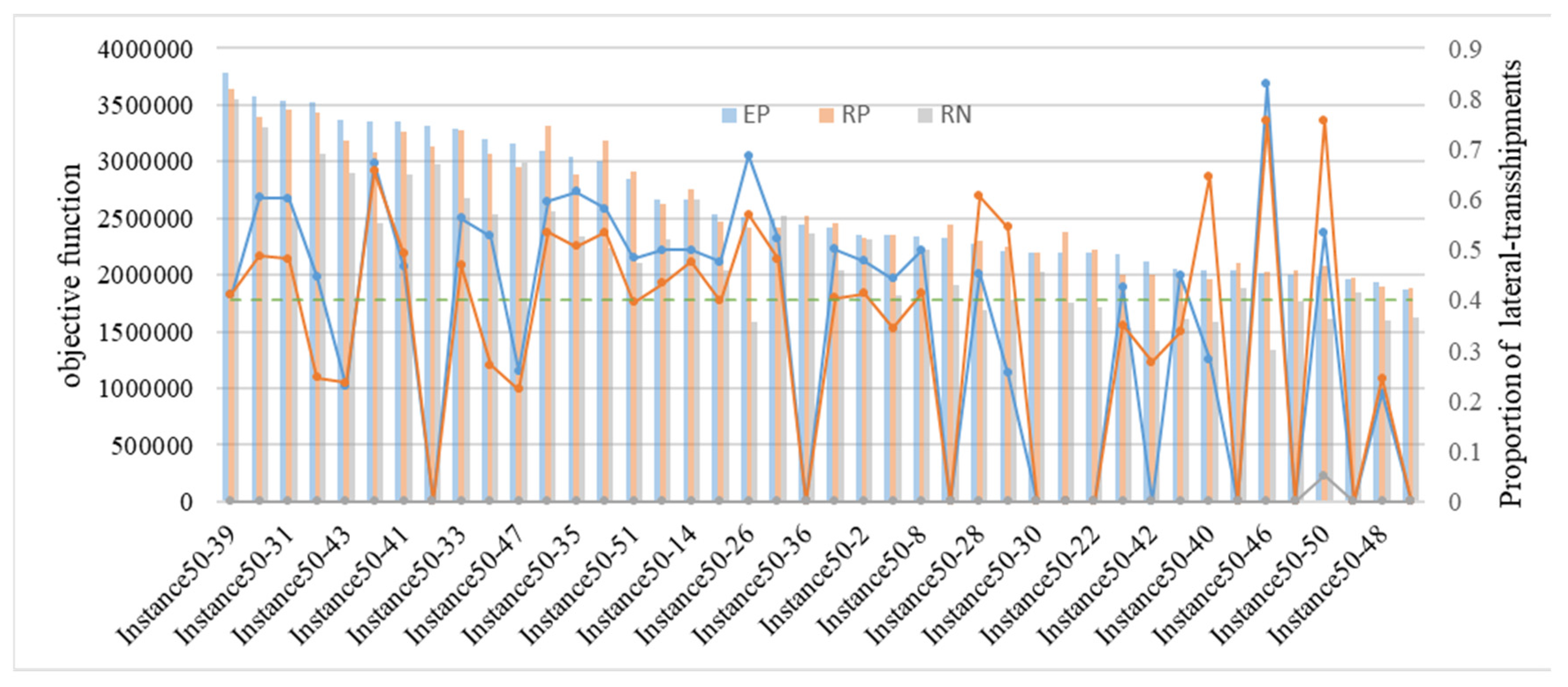
| DC | Warehouses Assigned to DC | Stations Covered by DC |
|---|---|---|
| 141 | 101; 102; 107; 108; 115; 129 | 4; 8; 37; 43; 57; 92; 94 |
| 142 | 110; 117; 121; 128; 132; 138 | 5; 34; 55; 68; 69; 87 |
| 143 | - | 12; 39; 51; 77 |
| 144 | 124; | 73 |
| 145 | 105; 119; 127; 134; 136; 137 | 2; 6; 7; 9; 10; 11; 17; 18; 25; 27; 28; 29; 30; 32; 33; 36; 40; 41; 45; 46; 54; 58; 64; 81; 82; 85; 93; 97; 98 |
| 146 | 106; 109; 111; 112; 116; 118; 122; 130; 139; 140 | 1; 3; 13; 14; 16; 19; 20; 21; 22; 31; 35; 48; 49; 50; 52; 56; 60; 61; 62; 67; 70; 72; 75; 76; 83; 89; 90; 96; 99; 100 |
| 147 | 104; 133 | 26; 65 |
| 148 | 114; 125 | - |
| 149 | 120; 135 | 15; 24; 38; 79; 80; 84; 95 |
| 150 | 103; 113; 123; 126; 131 | 23; 42; 44; 47; 53; 59; 63; 66; 71; 74; 78; 86; 88; 91 |
Disclaimer/Publisher’s Note: The statements, opinions and data contained in all publications are solely those of the individual author(s) and contributor(s) and not of MDPI and/or the editor(s). MDPI and/or the editor(s) disclaim responsibility for any injury to people or property resulting from any ideas, methods, instructions or products referred to in the content. |
© 2023 by the authors. Licensee MDPI, Basel, Switzerland. This article is an open access article distributed under the terms and conditions of the Creative Commons Attribution (CC BY) license (https://creativecommons.org/licenses/by/4.0/).
Share and Cite
Niu, Z.; Wu, S.; Zhou, X. Efficient Mathematical Lower Bounds for City Logistics Distribution Network with Intra-Echelon Connection of Facilities: Bridging the Gap from Theoretical Model Formulations to Practical Solutions. Algorithms 2023, 16, 252. https://doi.org/10.3390/a16050252
Niu Z, Wu S, Zhou X. Efficient Mathematical Lower Bounds for City Logistics Distribution Network with Intra-Echelon Connection of Facilities: Bridging the Gap from Theoretical Model Formulations to Practical Solutions. Algorithms. 2023; 16(5):252. https://doi.org/10.3390/a16050252
Chicago/Turabian StyleNiu, Zhiqiang, Shengnan Wu, and Xuesong (Simon) Zhou. 2023. "Efficient Mathematical Lower Bounds for City Logistics Distribution Network with Intra-Echelon Connection of Facilities: Bridging the Gap from Theoretical Model Formulations to Practical Solutions" Algorithms 16, no. 5: 252. https://doi.org/10.3390/a16050252
APA StyleNiu, Z., Wu, S., & Zhou, X. (2023). Efficient Mathematical Lower Bounds for City Logistics Distribution Network with Intra-Echelon Connection of Facilities: Bridging the Gap from Theoretical Model Formulations to Practical Solutions. Algorithms, 16(5), 252. https://doi.org/10.3390/a16050252