

Time Series Analysis by Fuzzy Logic Methods
 ,
, 
Abstract
1. Introduction
2. Materials and Methods
2.1. DMA–Morphological Analysis: Nonformal Logic
2.1.1. Elementary Measures
2.1.2. Morphological Measures
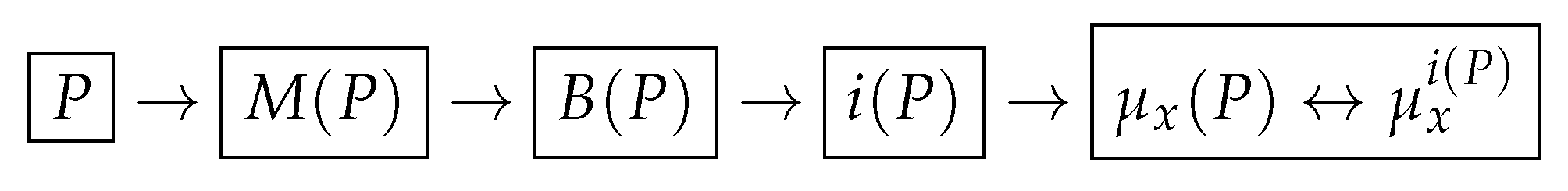
2.1.3. Conversion of the Geometry of One-Dimensional Relief into the Language of Fuzzy Logic
- −
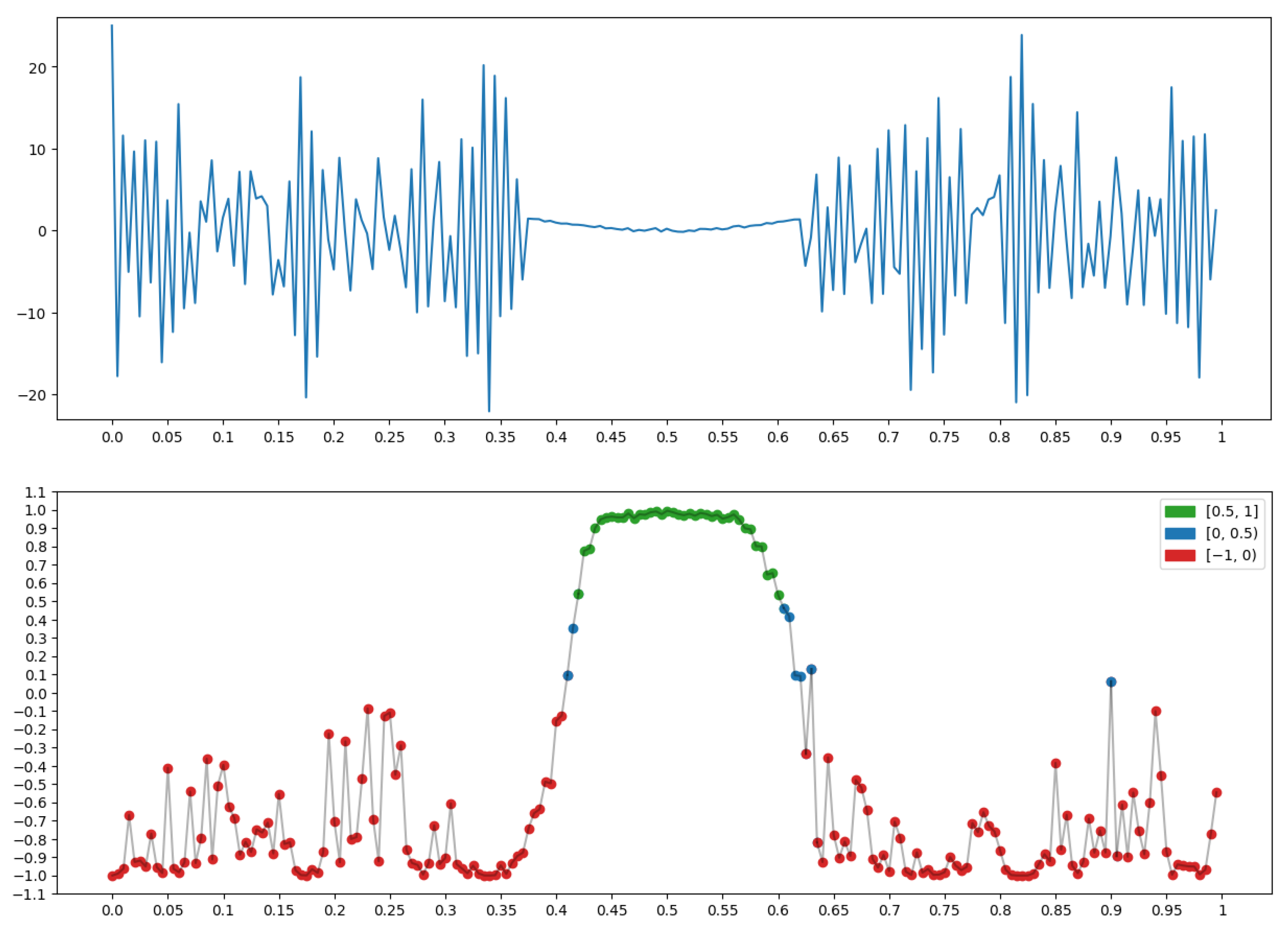
- It is difficult to say how geometric a record x appears in the region of node t with condition , but the situation is clear, which is “evenness” on the record x near node t in context ∗.
- −
- A large value of any measure (2) is equivalent to large values of all the terms included in its ⋀-conjunction.
P: “Background” for x at Node t

P: “Beginning of Growth (Mountain)” for x at Node t

P: “End of Recession (Mountain)” for x at Node t

P: “Beginning of a Plateau” for x at Node t

P: “End of Plateau” for x at Node t

P: “Climb (Rise)” for x at Node t

P: “Decline (Decrease)” for x at Node t

P: “Peak (Top)” for x at Node t

P: “Depression (Bottom)” for x at Node t

P: “Left Oscillation” for x at Node t

P: “Right Oscillation” for x at Node t

P: “Right Oscillation with Left Increase” for x at Node t

P: “Right Oscillation with Left Decrease” for x at Node t

P: “Left Oscillation with Right Decrease for x at Node t

P: “Left Oscillation with Right Increase” for x at Node t

P: “Two-Way Oscillation” for x at Node t

2.1.4. Conclusions
2.2. Next Steps
- −
- the first part involves extracting knowledge about the record by constructing morphological measures based on Section 2.1.3;
- −
- the second part focuses on improving the quality of conversion from one-dimensional relief geometry to fuzzy logic language according to the same Section 2.1.3;
- −
- the third part is similar to the first, but involves more complex scenarios where morphological measures are combined with other approaches to study the original record.
- −
- Reason one is that the kernel of the measure consists of exactly the nodes where at least one of the elementary measures . is equal to zero. In this way,
- −
- Reason two is that, in the general case, and taking into account the large number of nodes , and the stochasticity of x, we can conclude that the kernels are small (“measure zero”) in T, and, therefore, their union is small in T.
2.3. DMA-Morphological Analysis: Formalization
2.3.1. Background
2.3.2. Beginning of Growth (Mountain)
2.3.3. End of Descend (Mountain)
2.3.4. Beginning of Plateau
2.3.5. End of Plateau
2.3.6. Climb (Growth)
2.3.7. Descending (Decreasing)
2.3.8. Peak (Top)
2.3.9. Depression (Bottom)
2.3.10. Left Oscillation
2.3.11. Right Oscillation
2.3.12. Right Oscillation with Left Increase
2.3.13. Right Oscillation with Left Decrease
2.3.14. Left Oscillation with Right Decrease
2.3.15. Left Oscillation with Right Increase
2.3.16. Two-Way Oscillation
2.3.17. Morphological Analysis
2.3.18. Conclusions
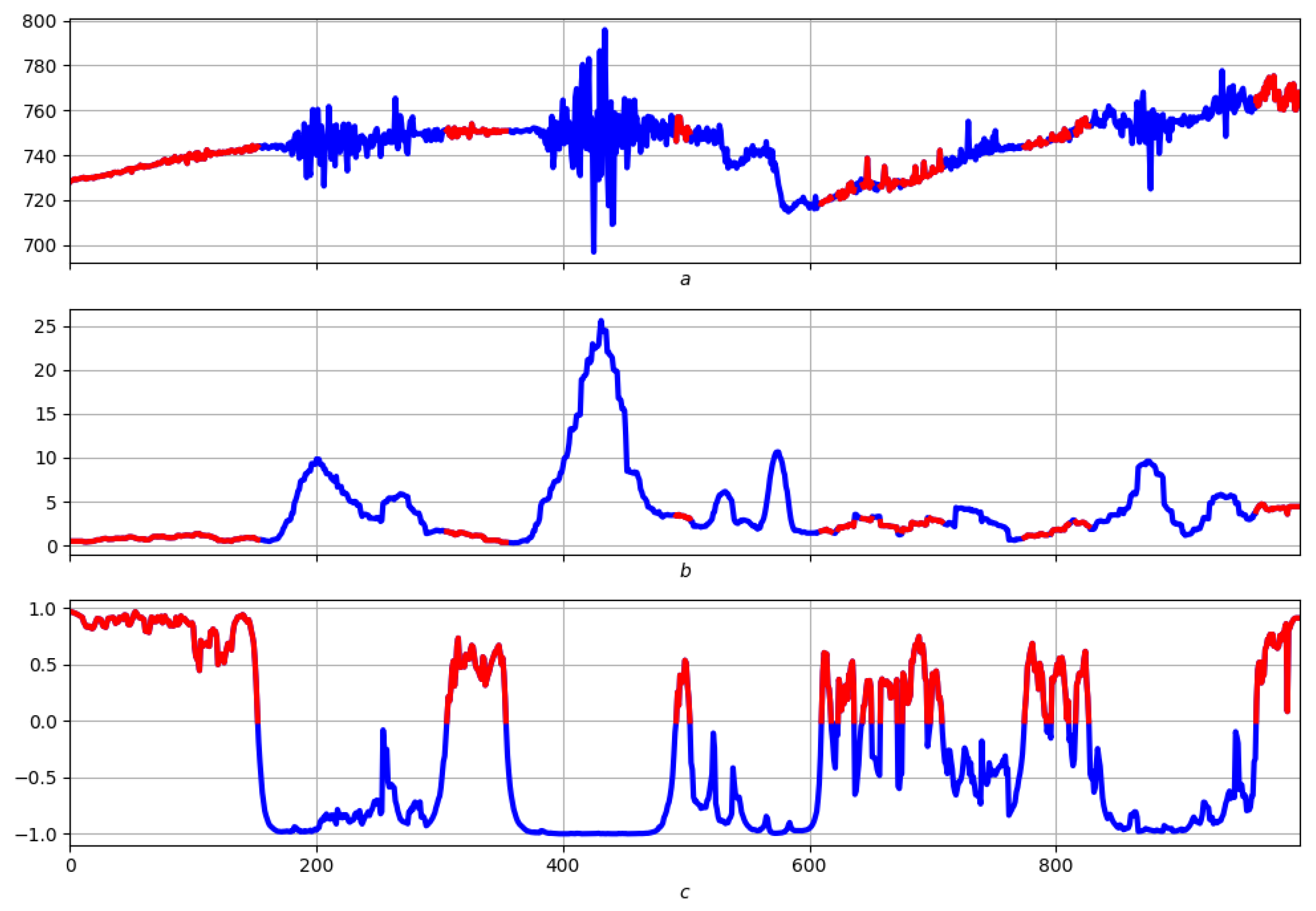
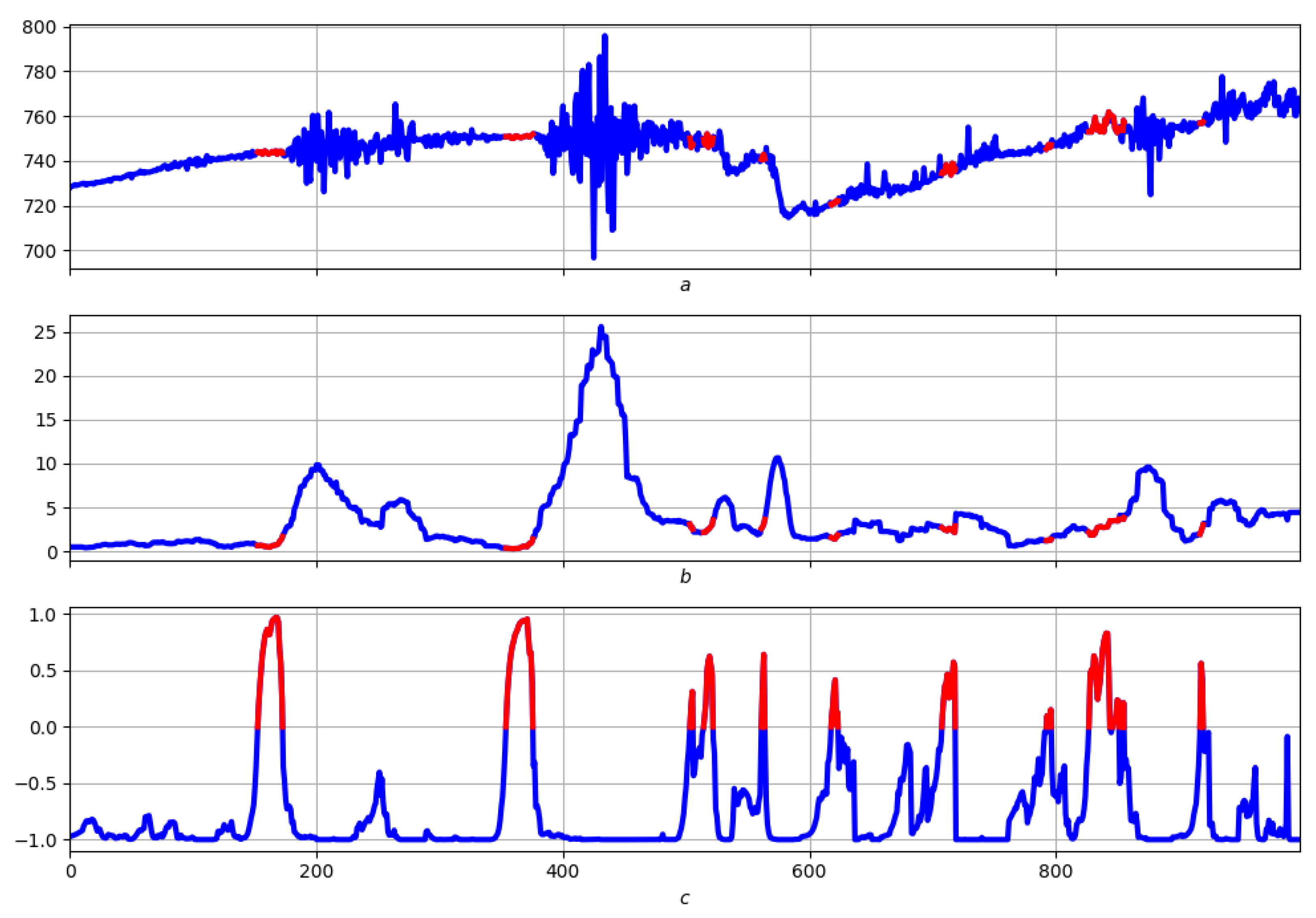
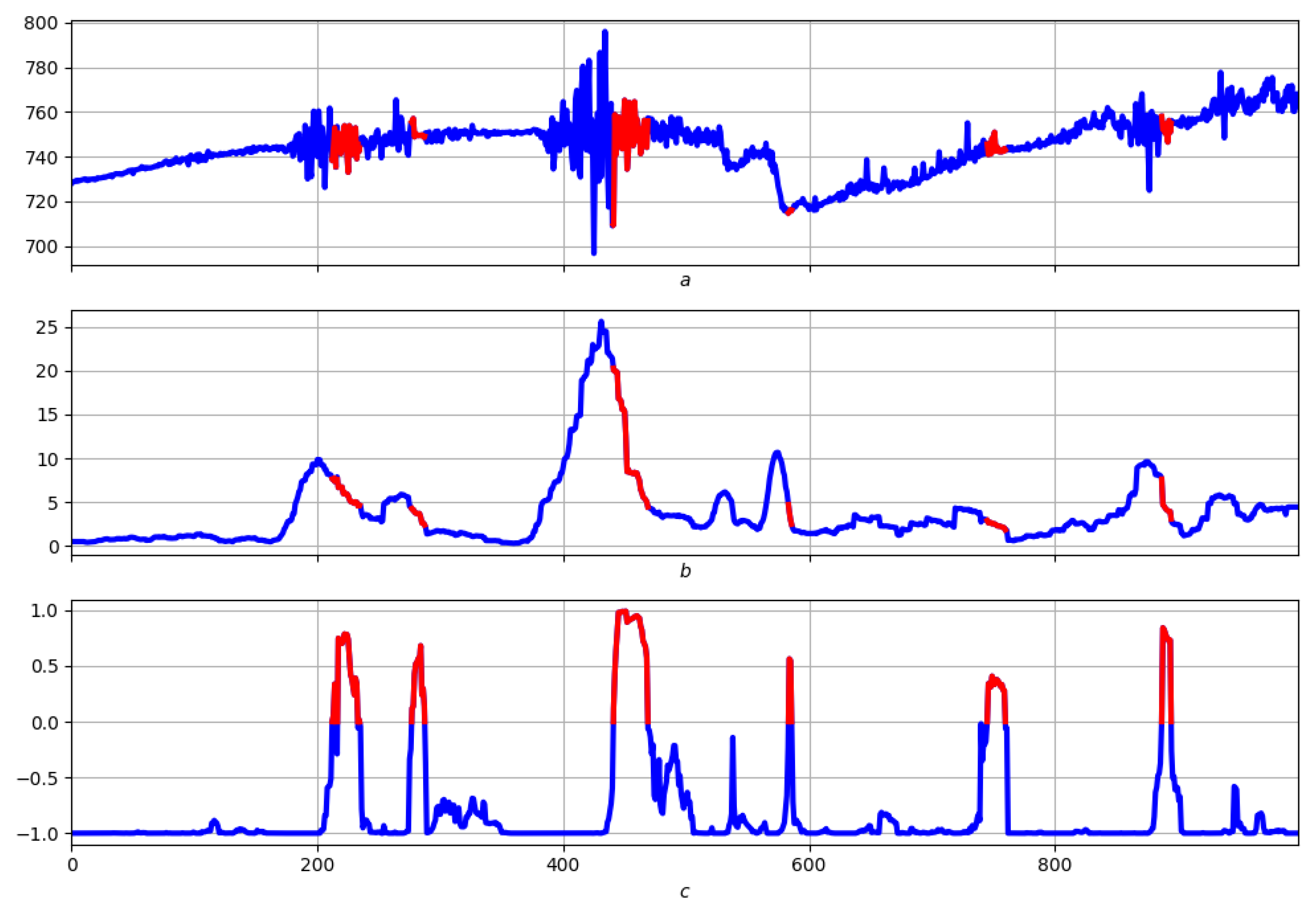
3. -Morphological Analysis
3.1. Record Straightening
3.1.1. Definition
- 1.
- The straightening construction R is a non-negative functional on T, parameterized by T:
- 2.
- The straightening of x, based on the construction R, is a non-negative function .
3.1.2. Conclusions
3.2. R-Morphological Measures
4. Search for Elevations Using Morphological Measures
4.1. Required Minimum: Designations, Definitions, Facts
4.1.1. Definition
4.1.2. Statement
4.1.3. Definition
4.1.4. Definition
4.1.5. Statement
4.1.6. Notations
4.1.7. Conclusions
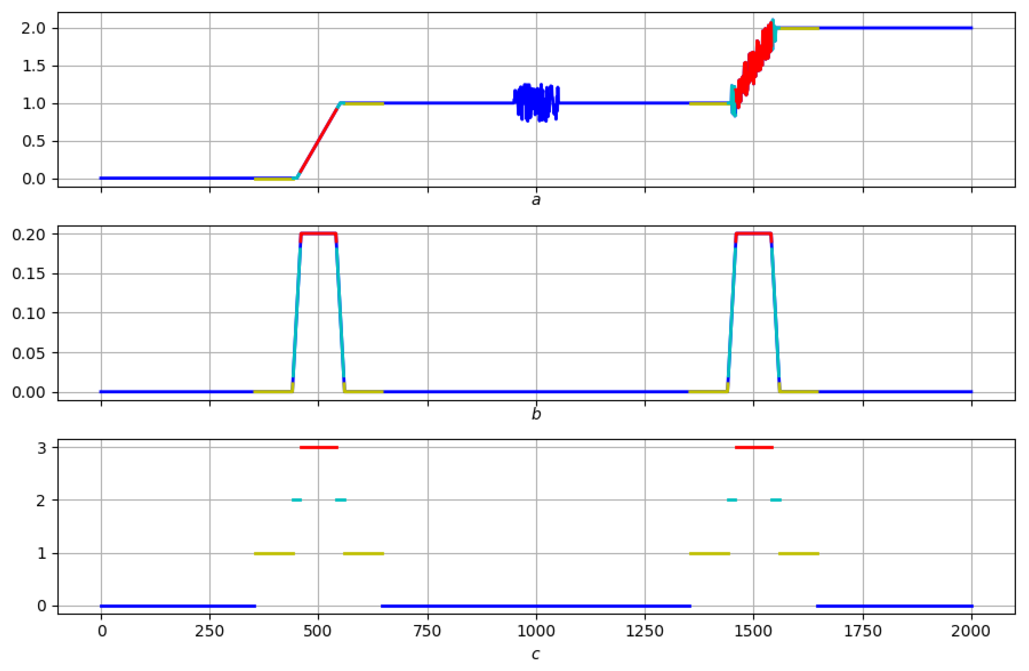
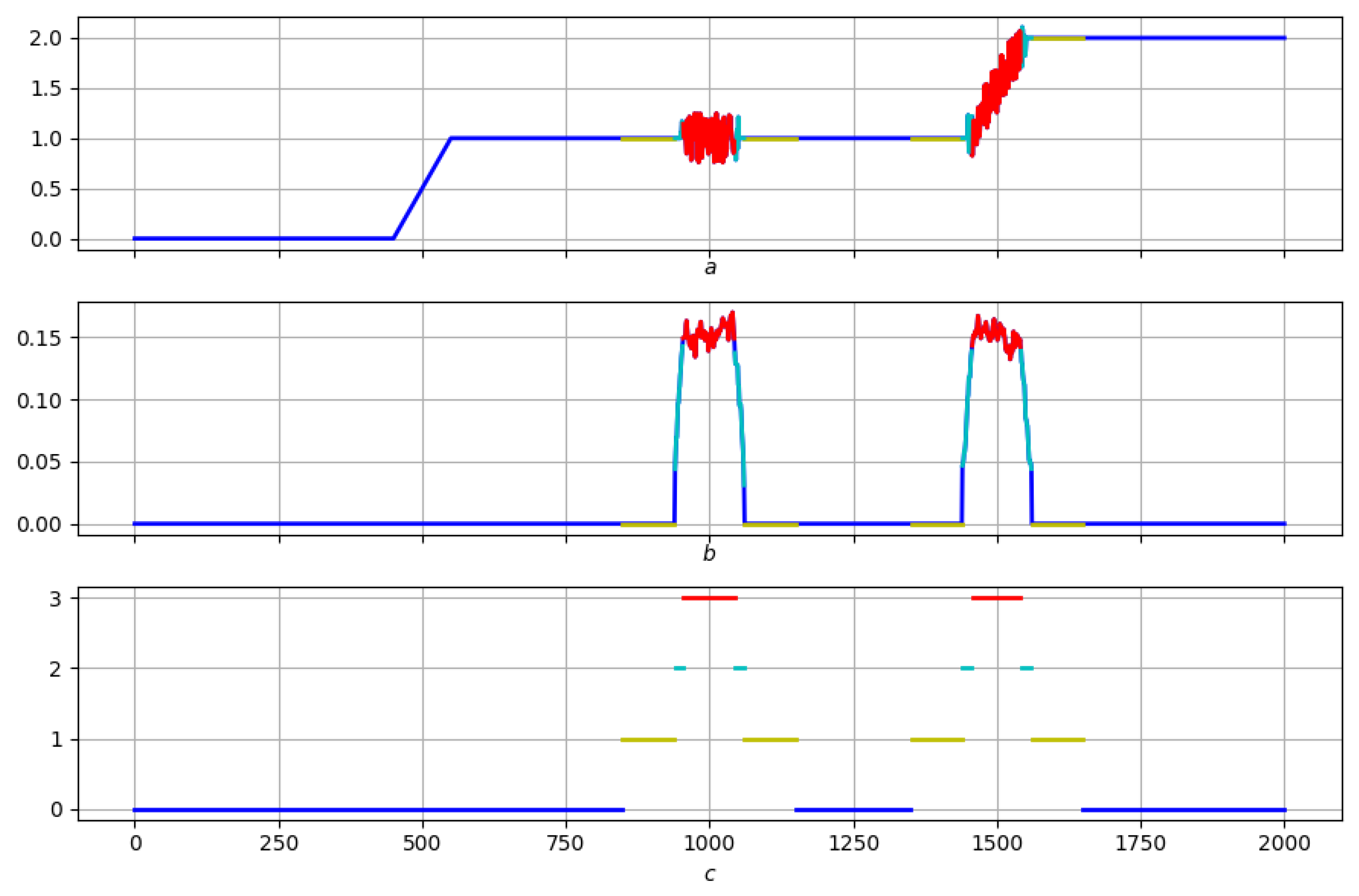
4.2. Search Algorithm: Logic and Formalization
4.2.1. Construction of Elevation
4.2.2. Logic of the Initial Stage
4.2.3. Formalization of the Initial Stage
4.2.4. End Stage Logic
4.2.5. Formalization of the Final Stage
4.2.6. The Logic of the Central Part
4.2.7. Formalization of the Central Part
4.2.8. Left Slope
4.2.9. Right Slope
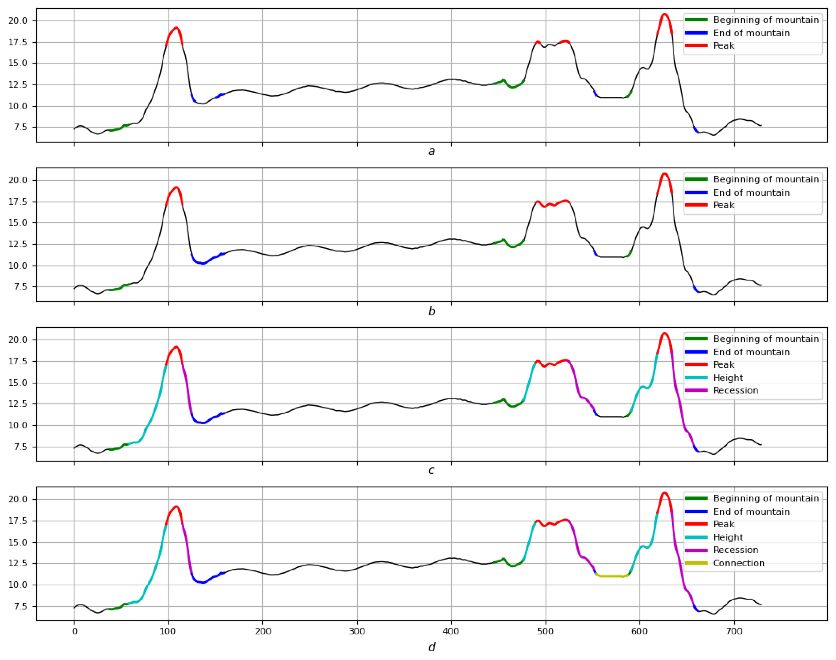
4.2.10. Elevations and Their Chains
4.2.11. Conclusions
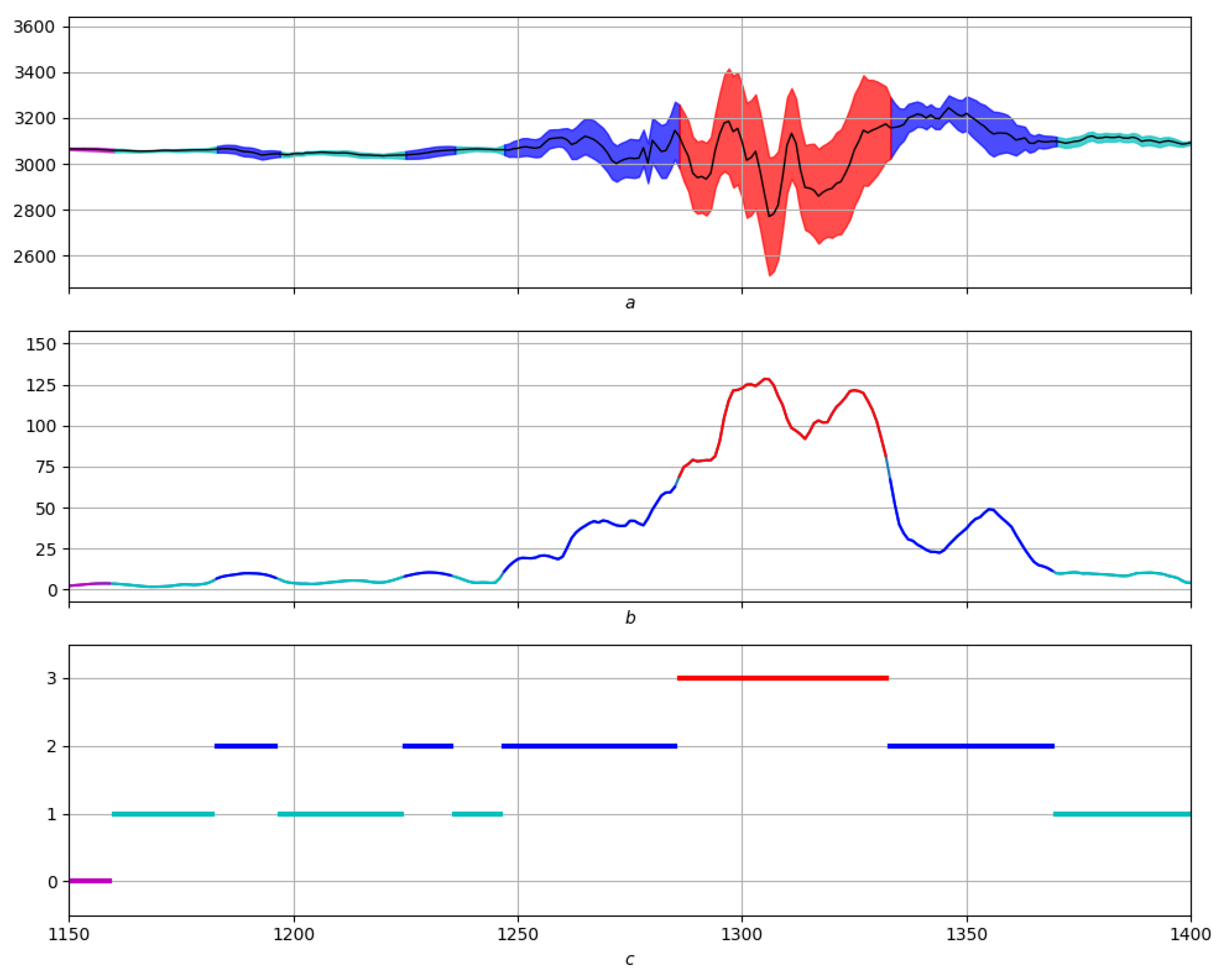
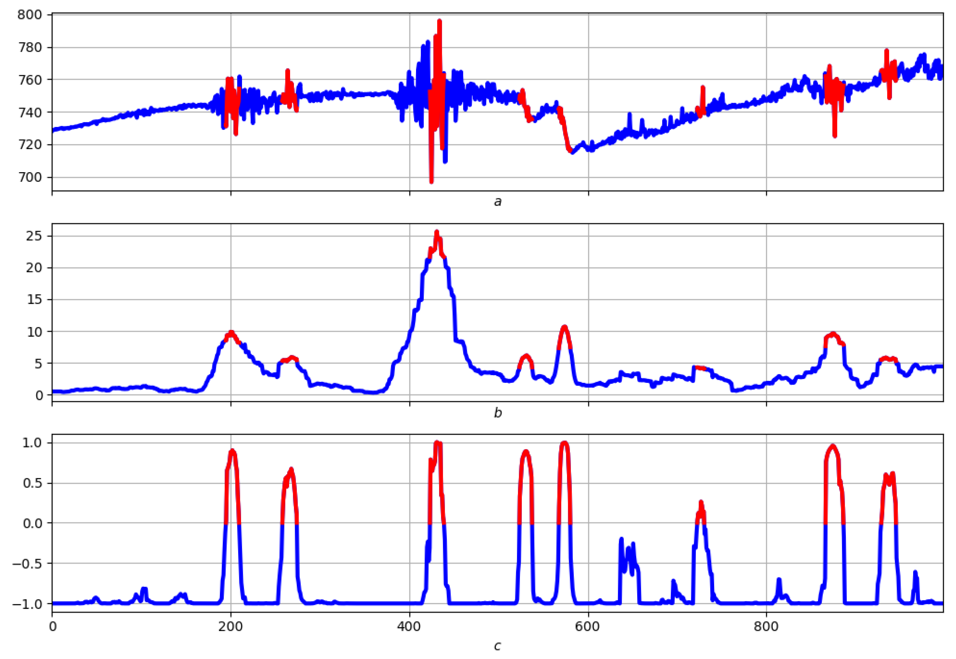
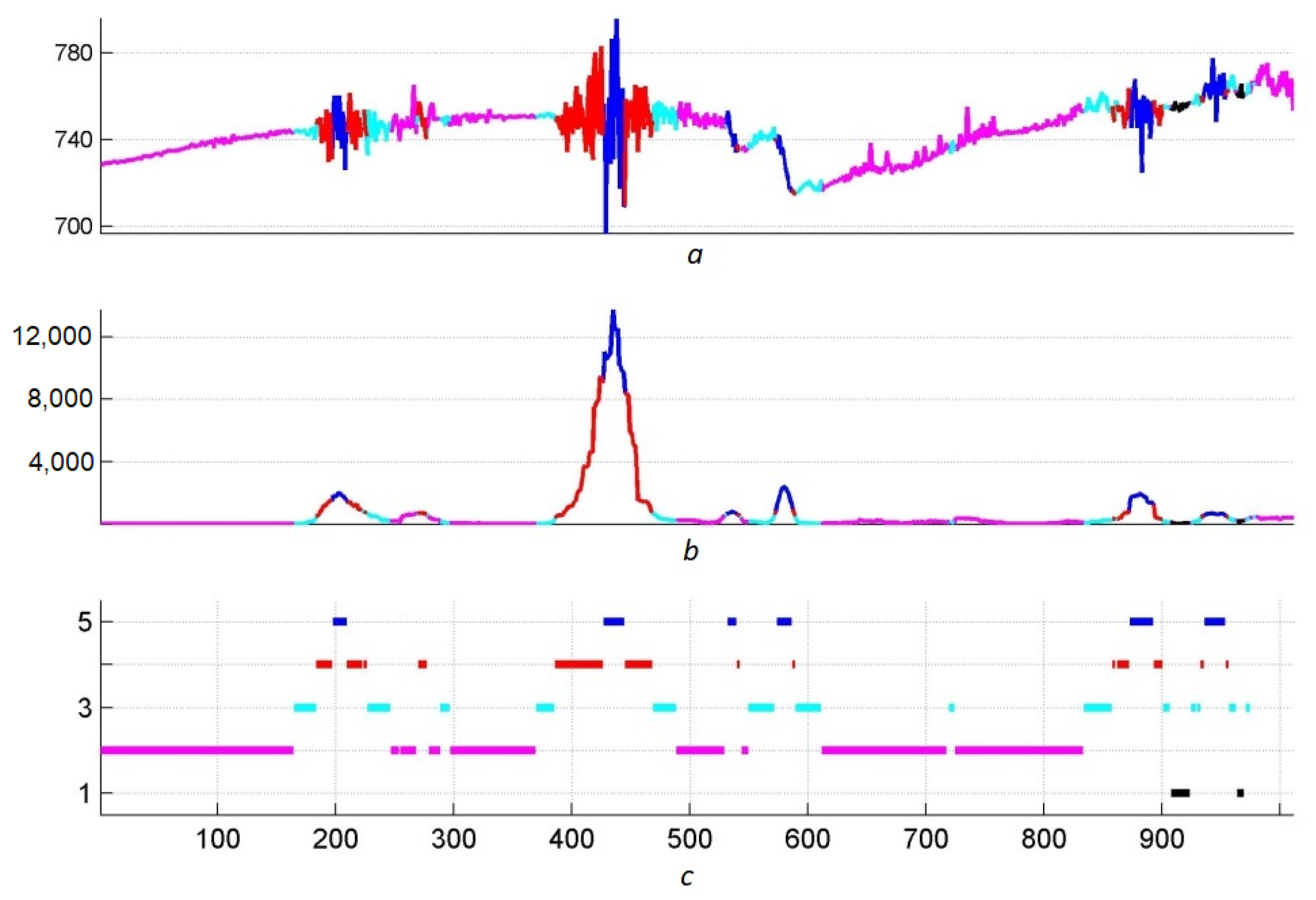
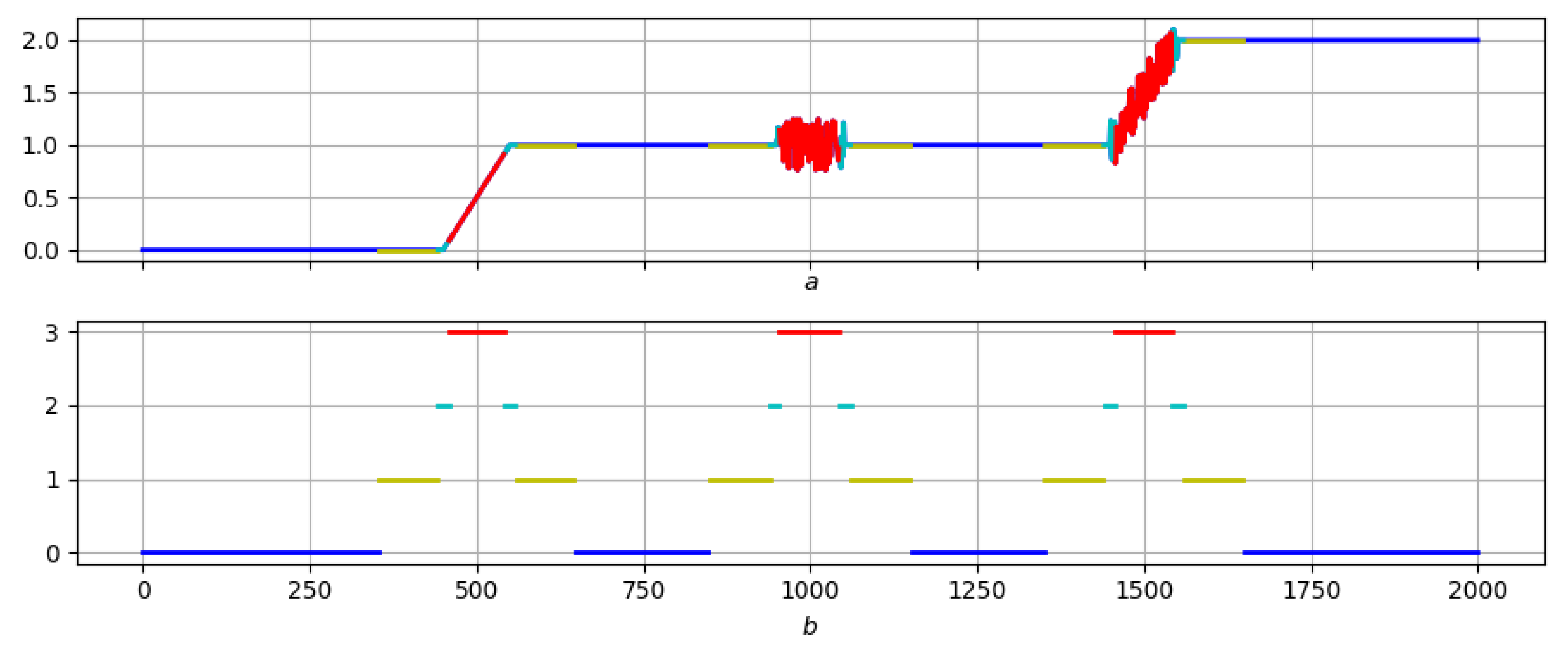
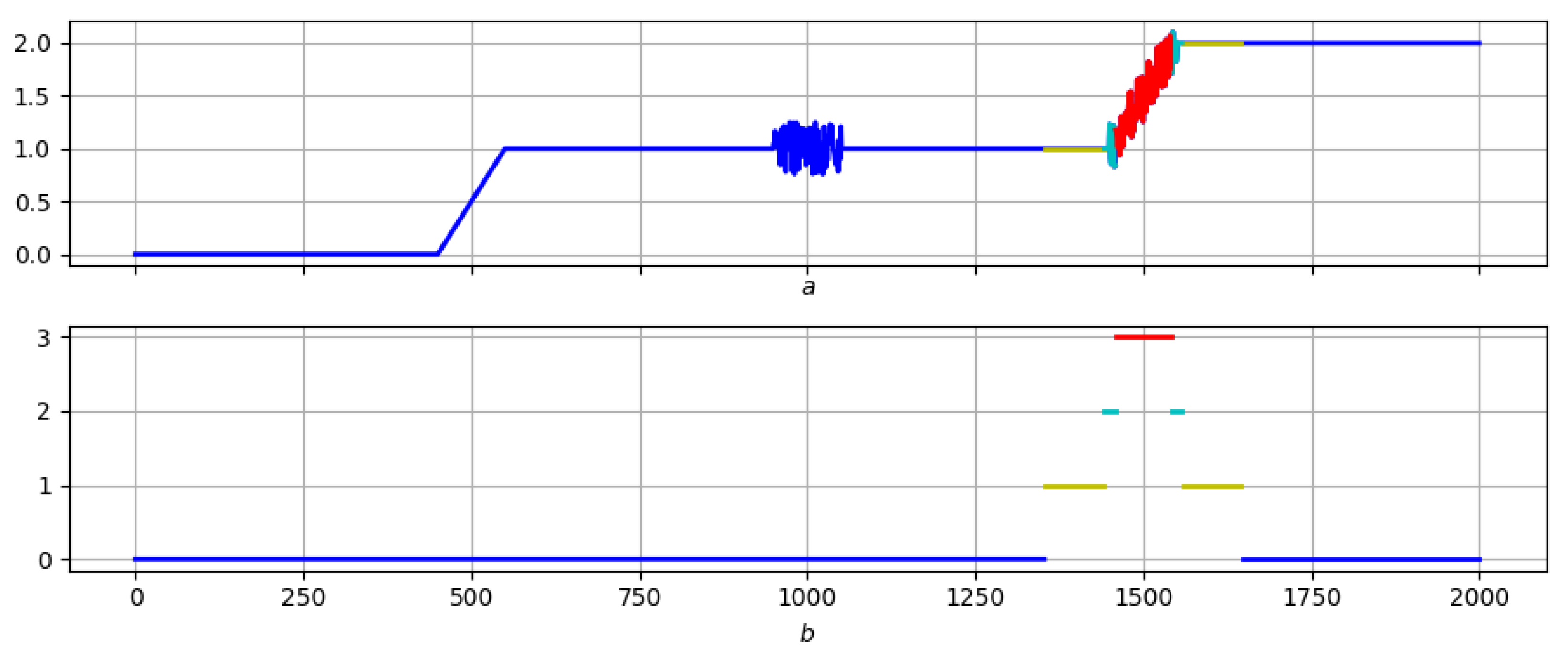
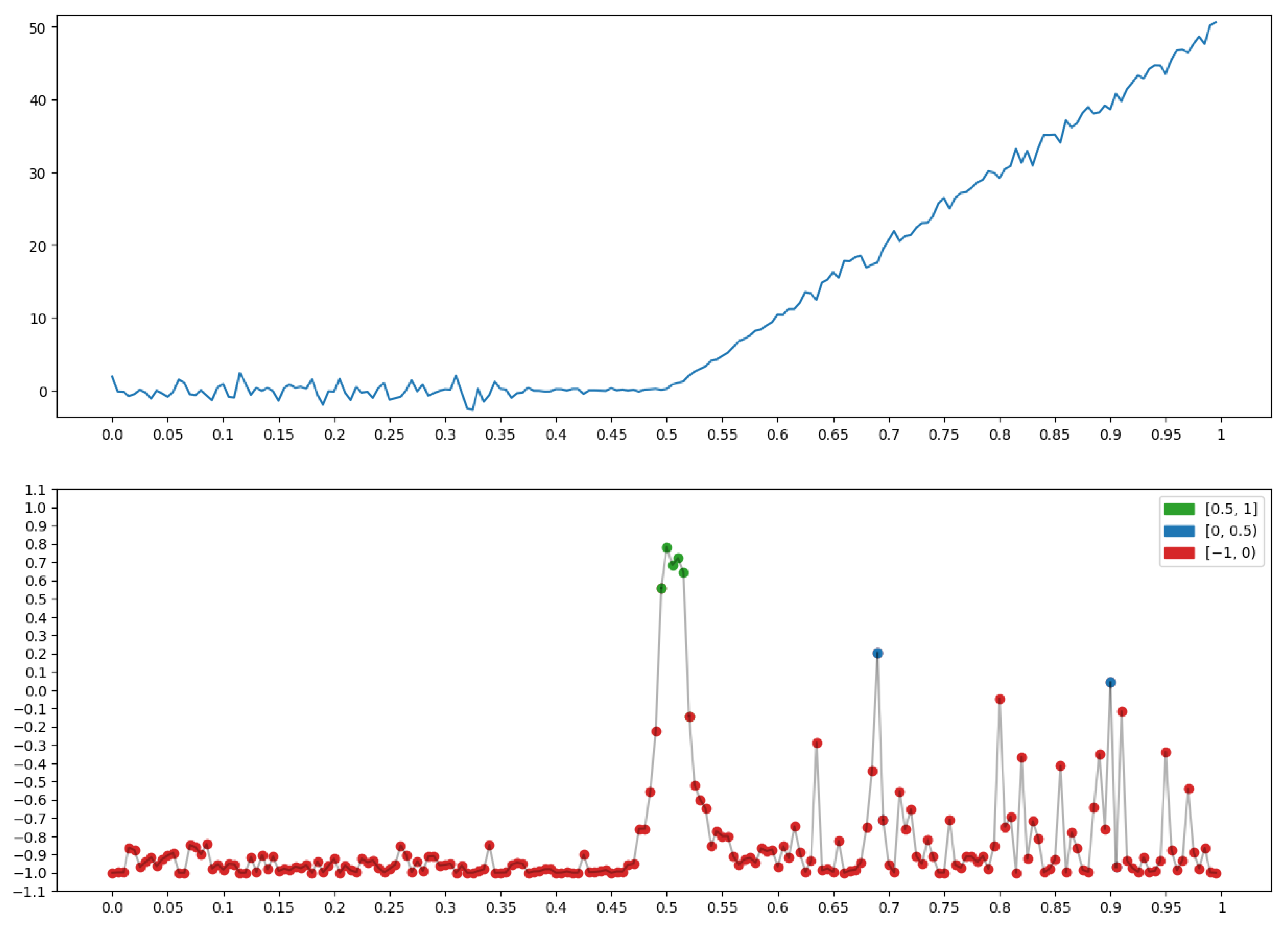
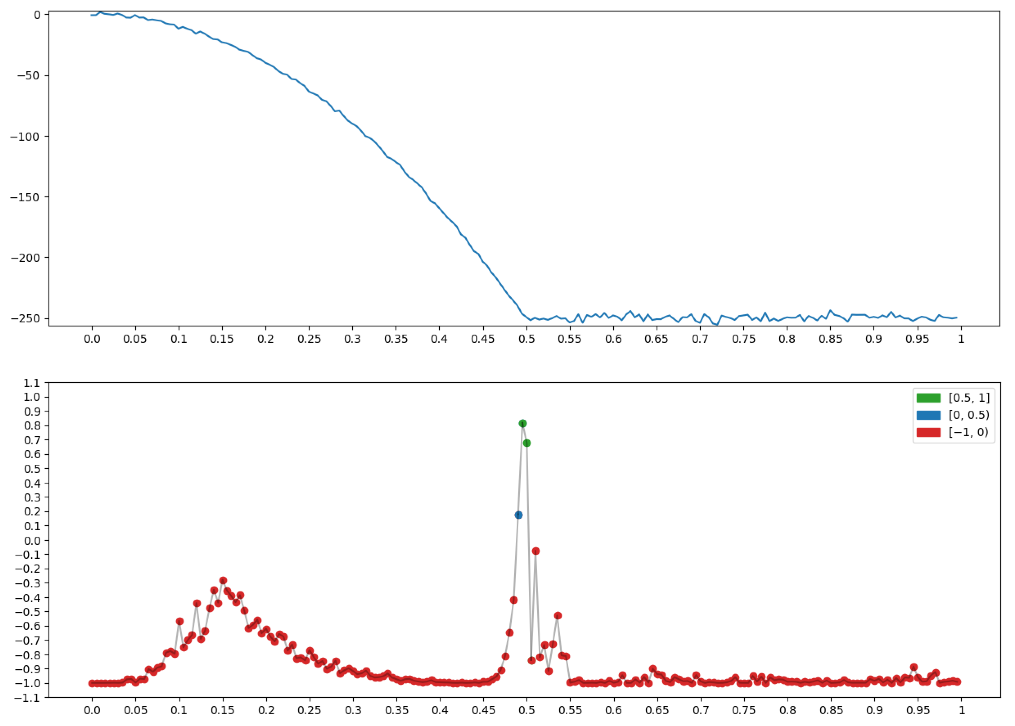
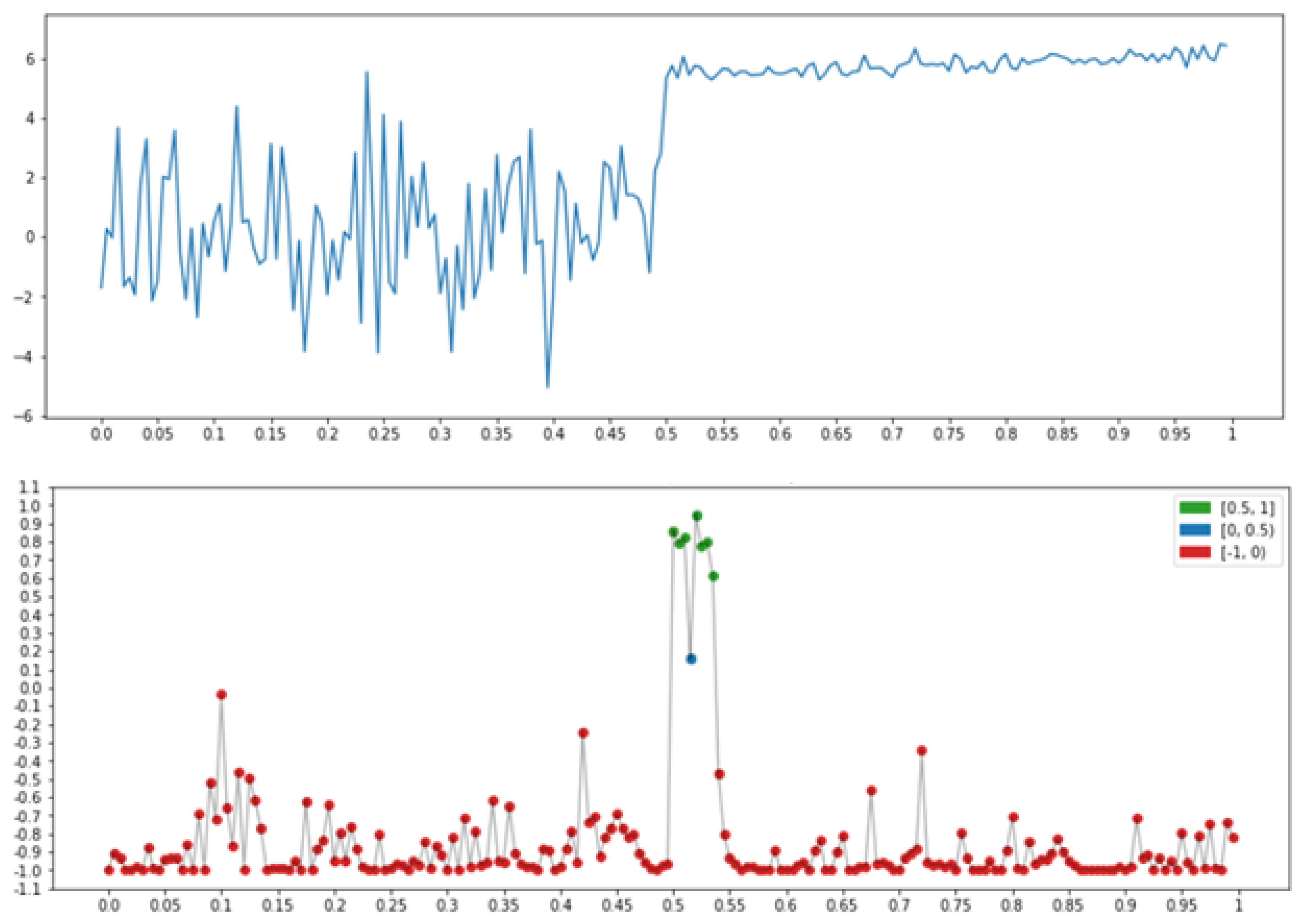
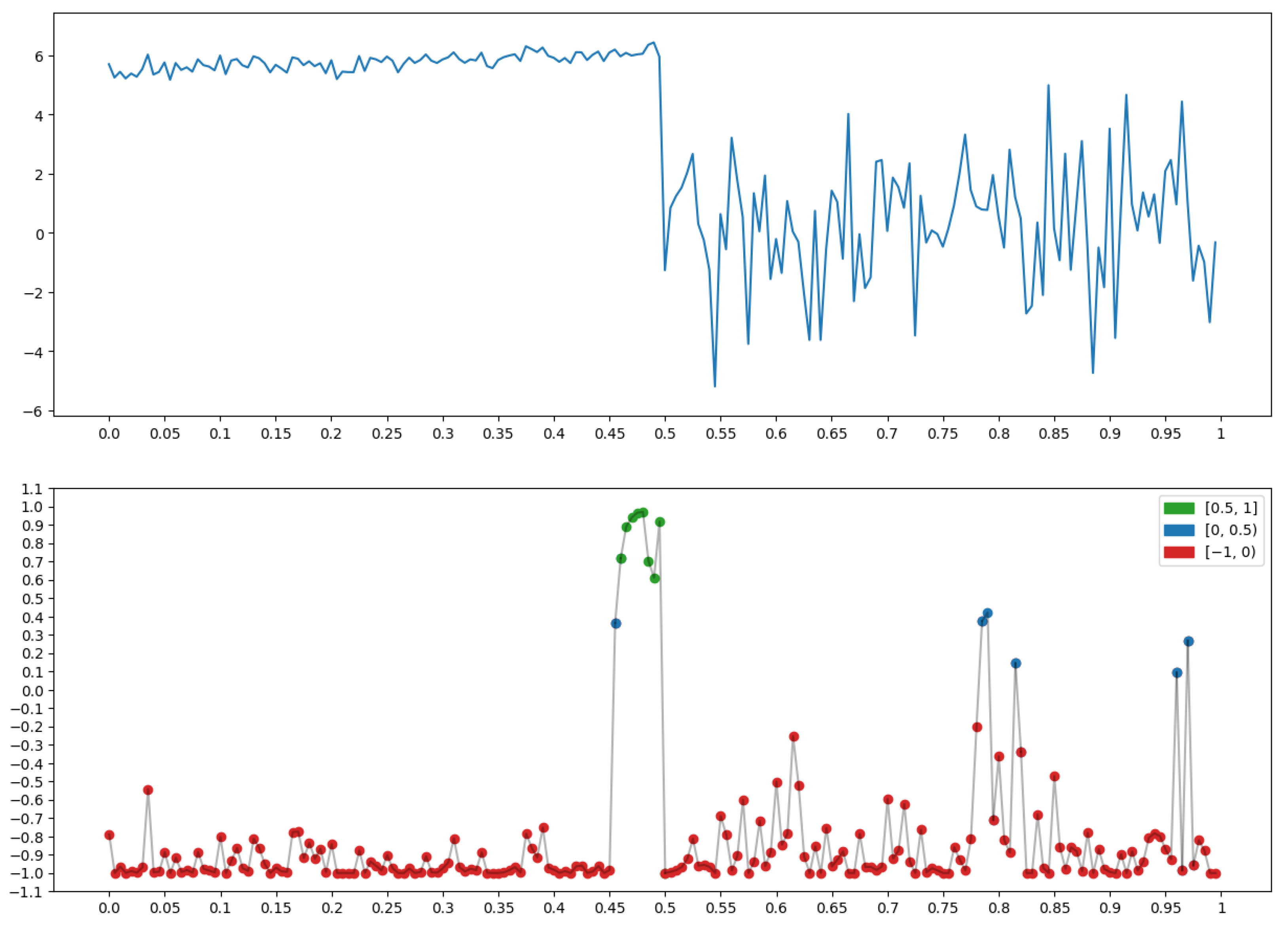
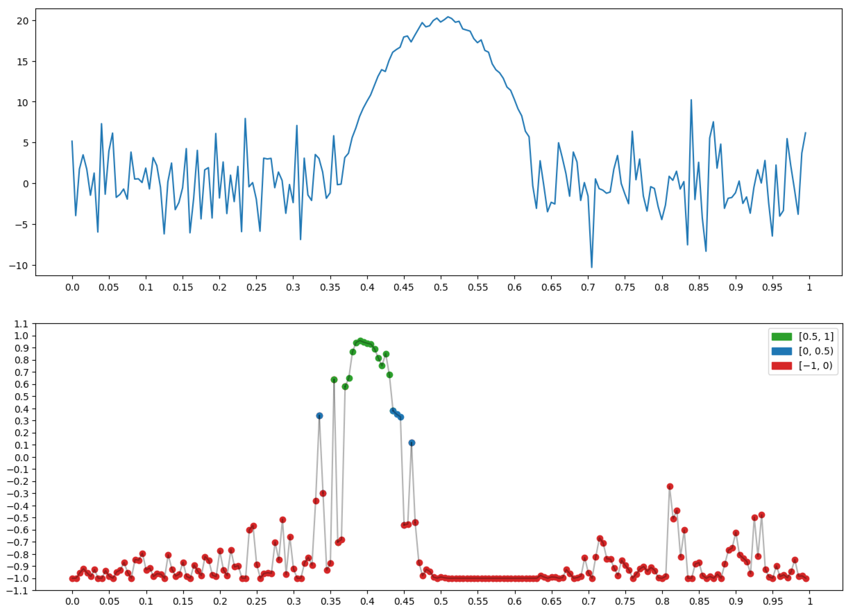
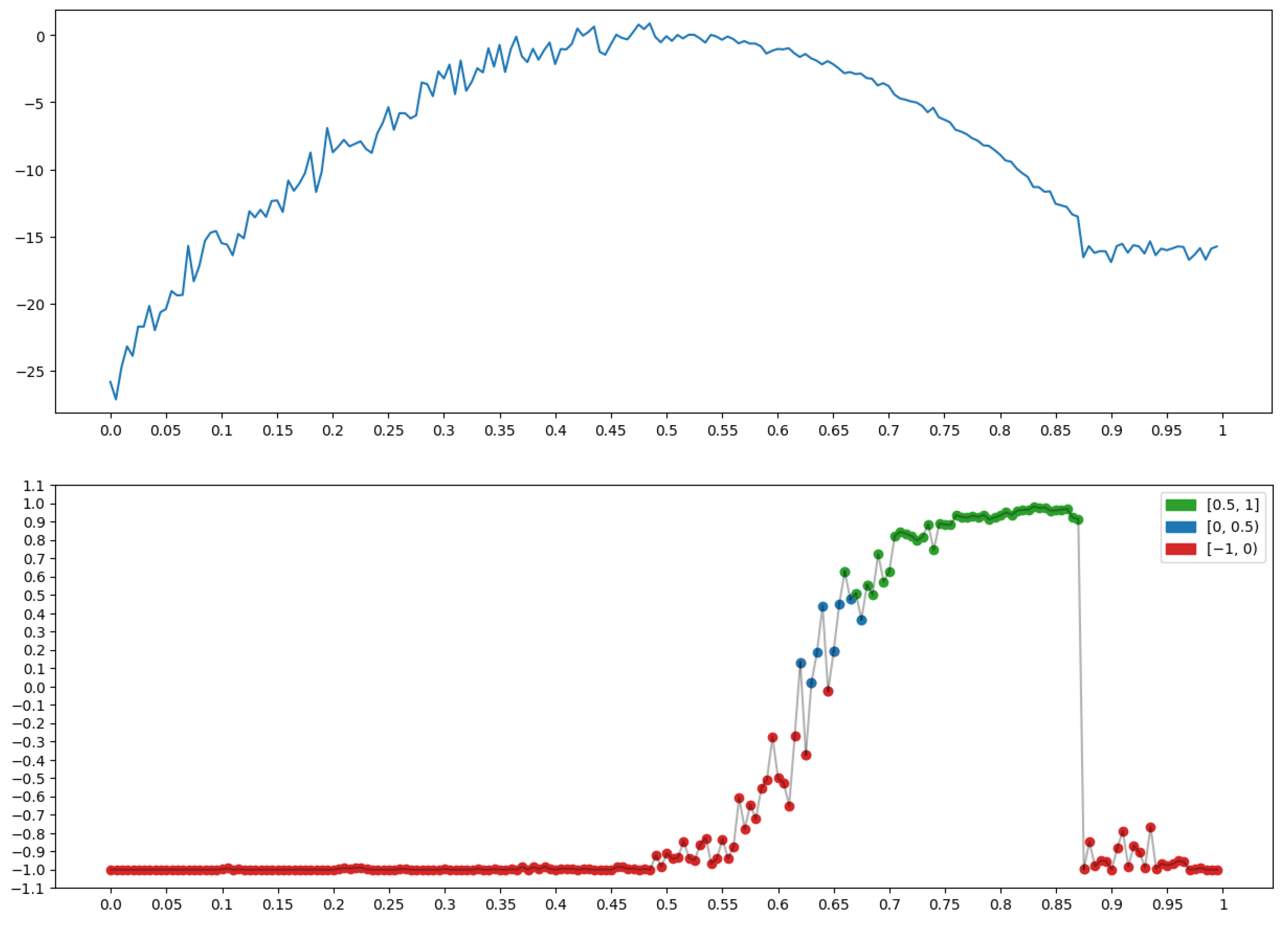
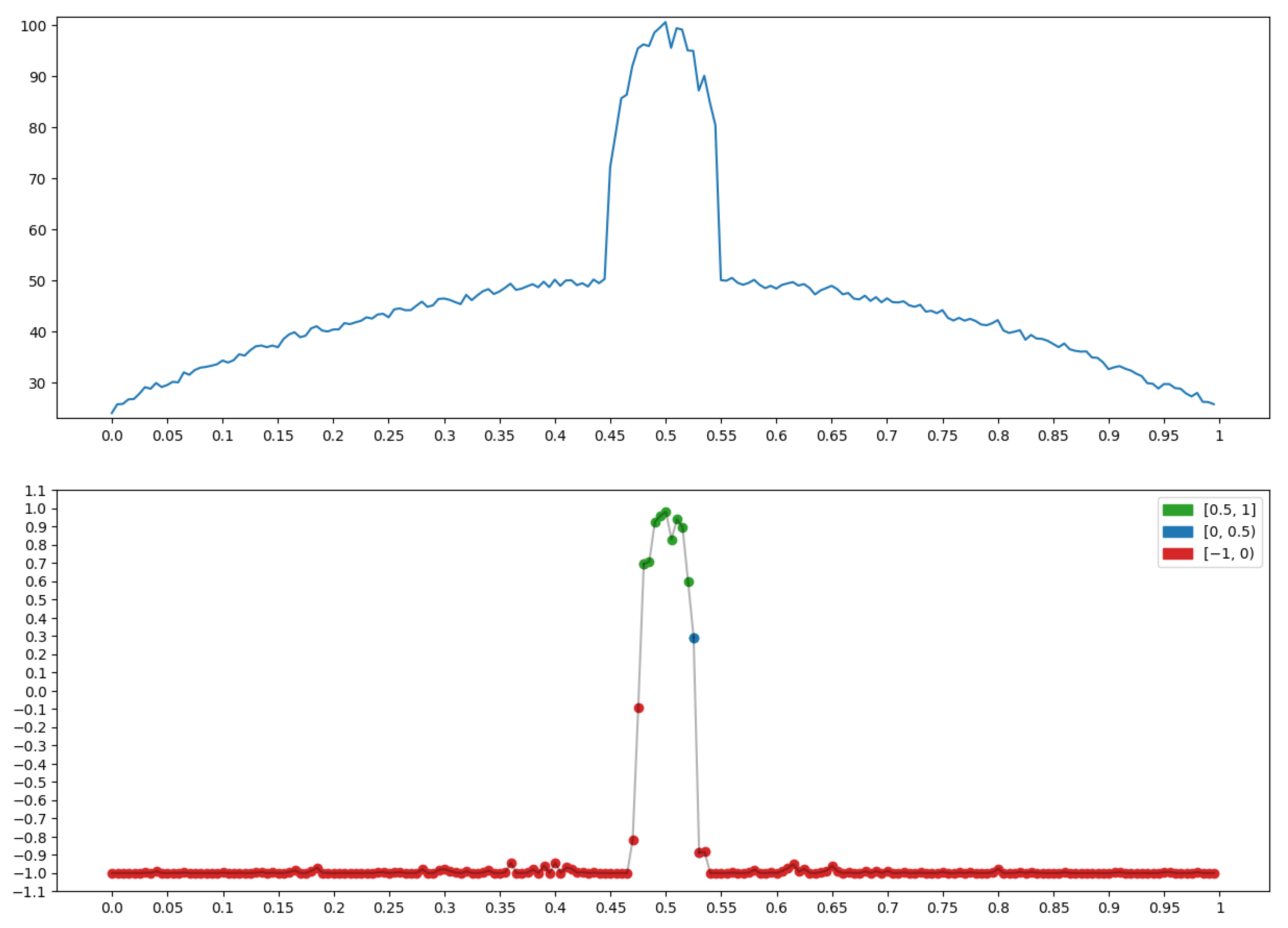
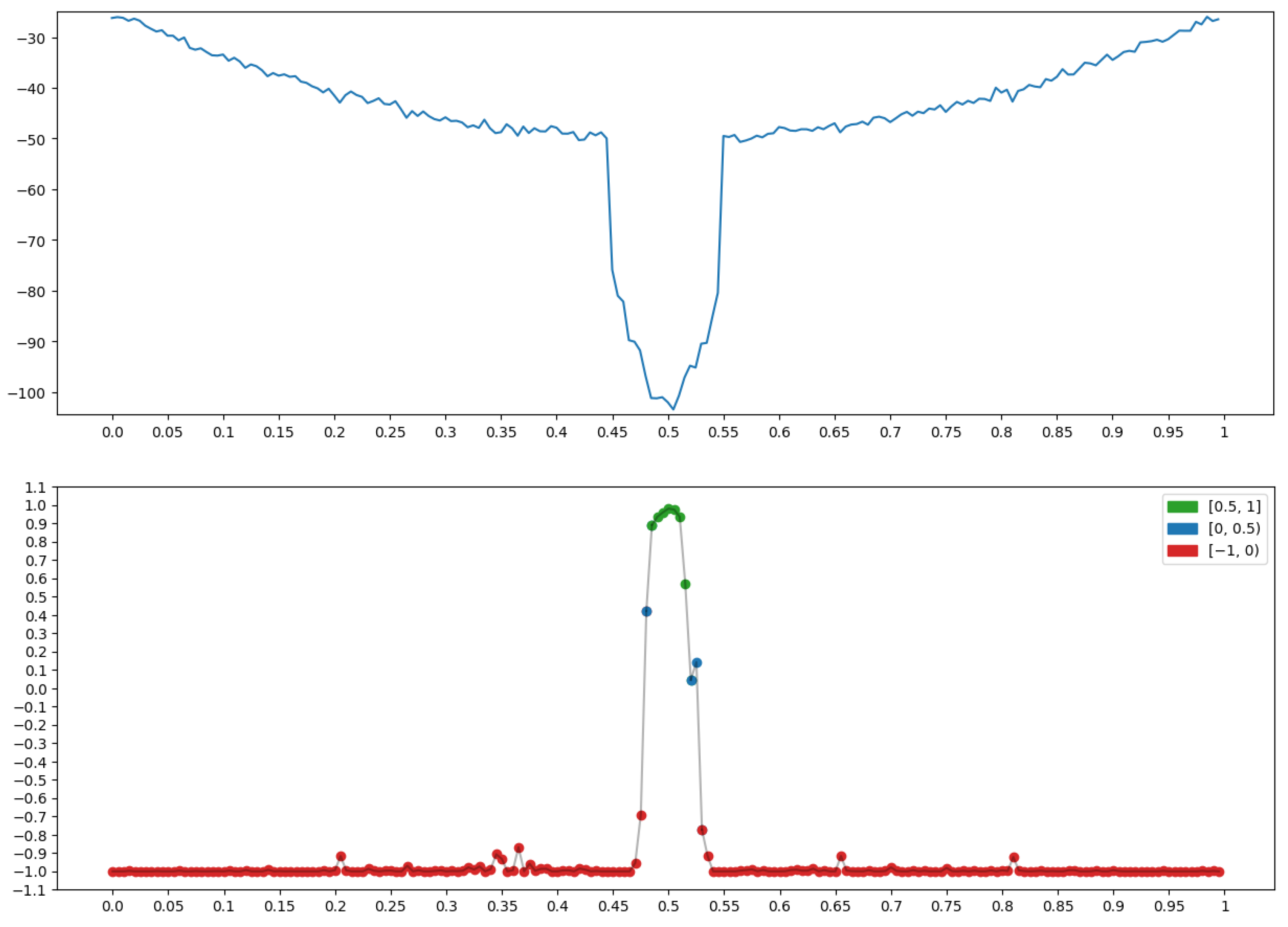
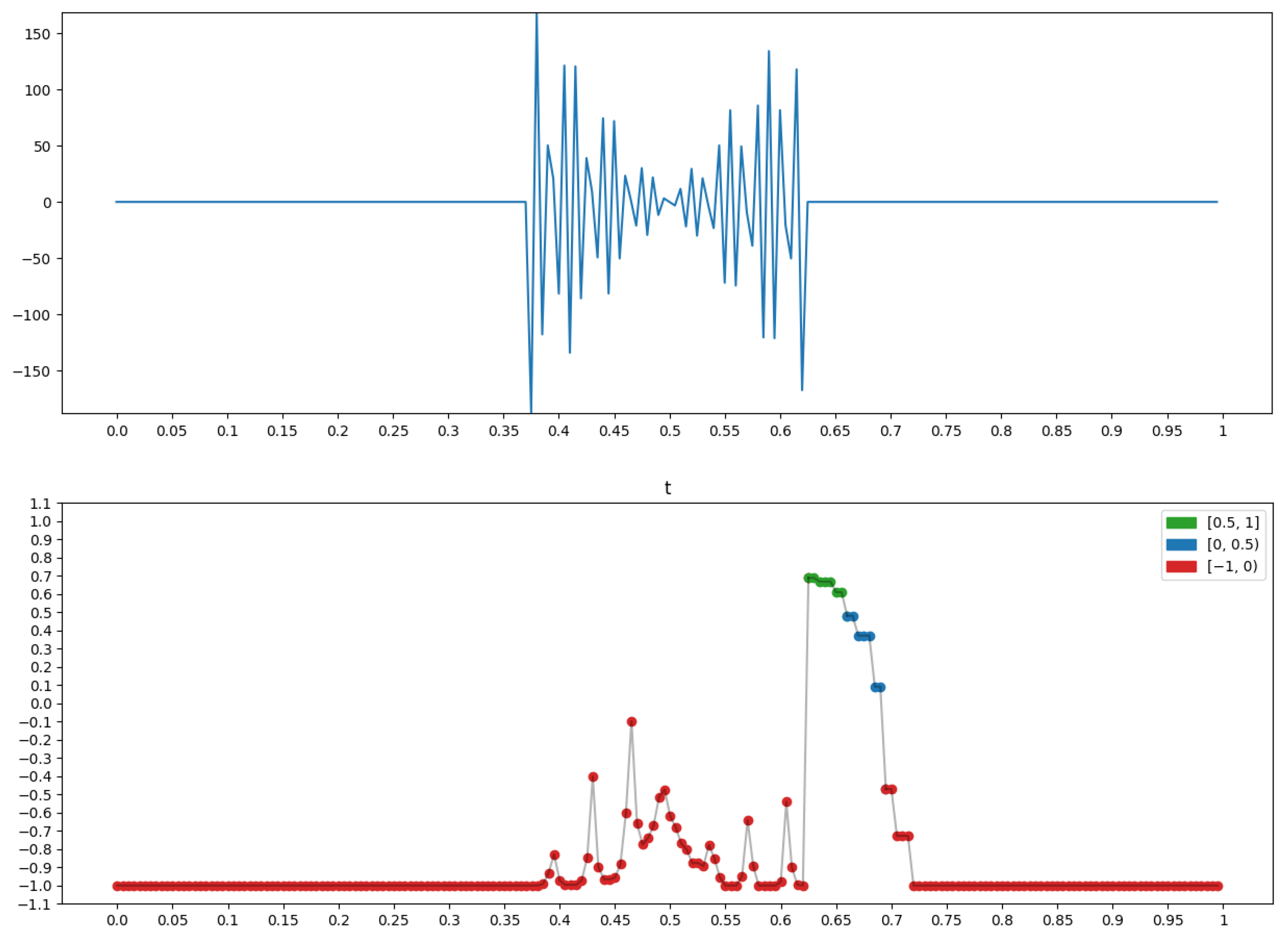
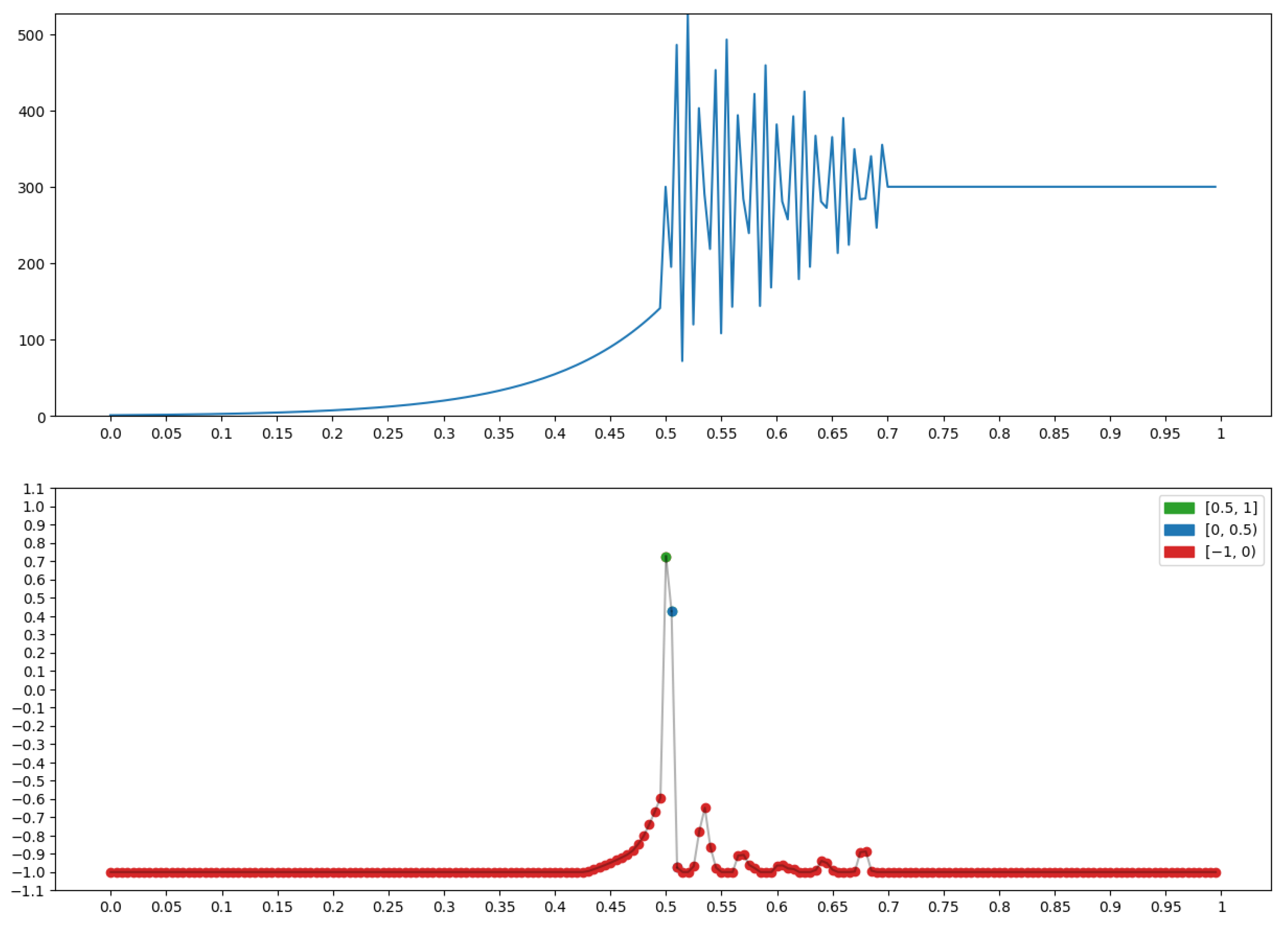
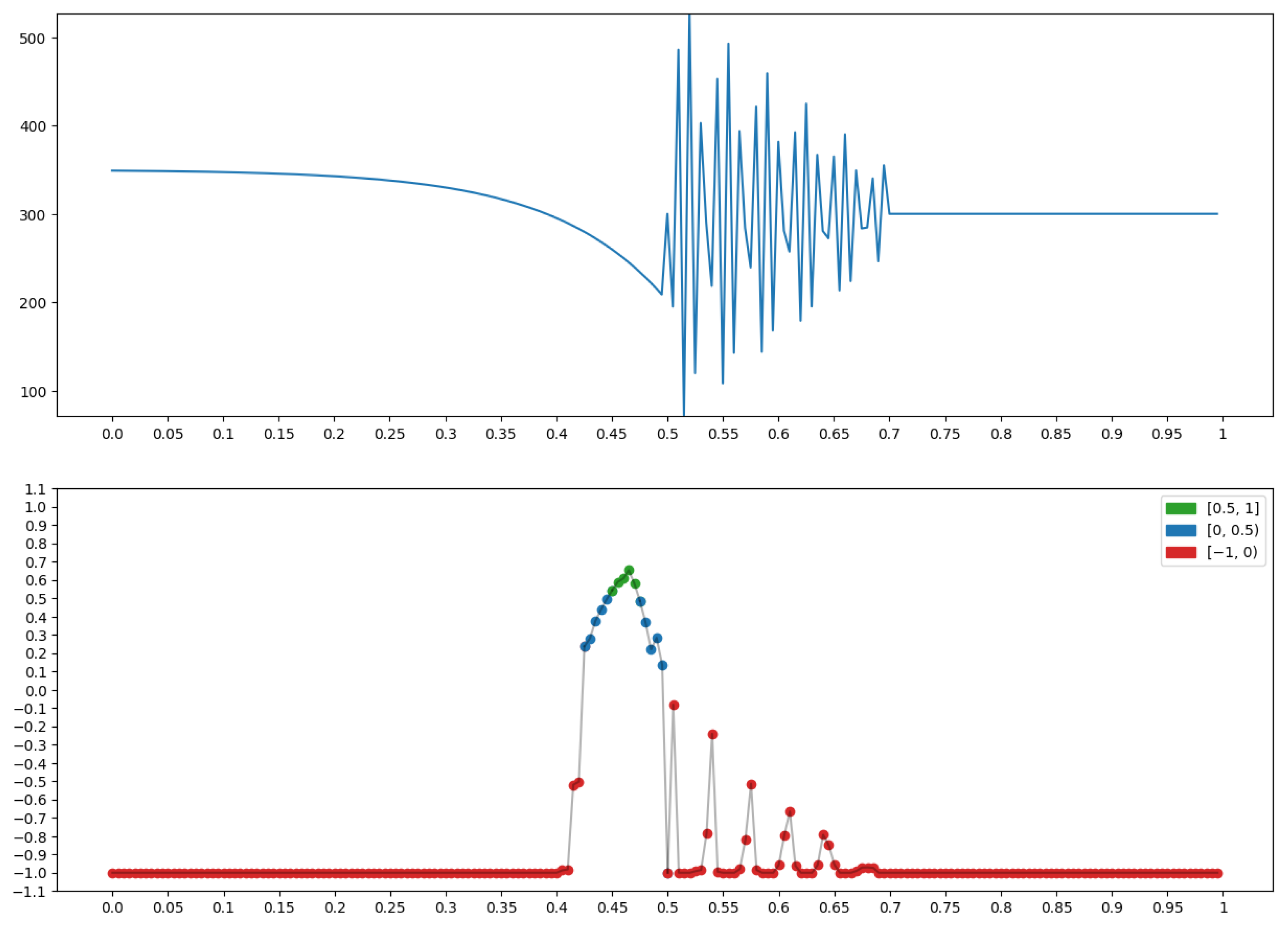
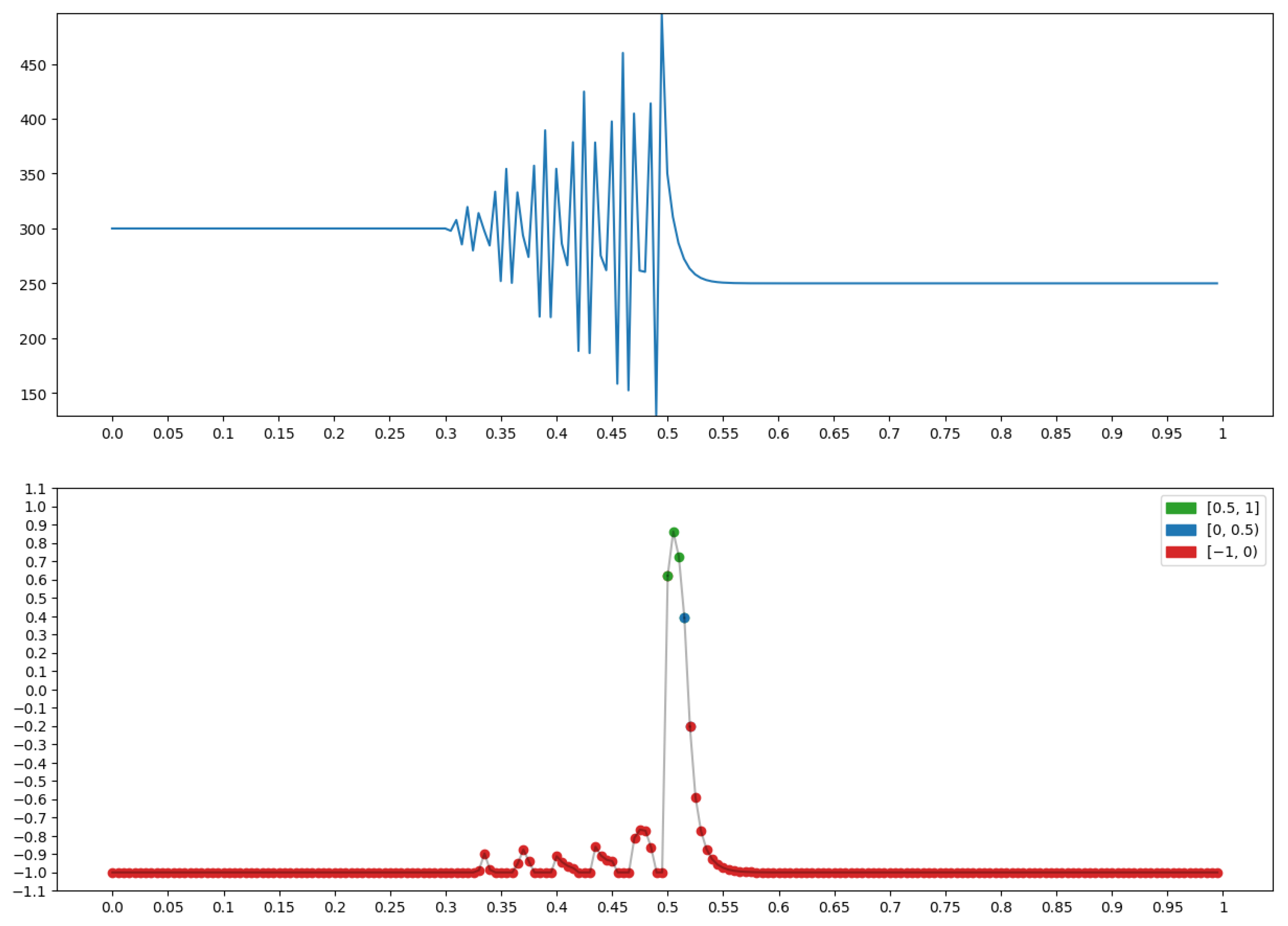
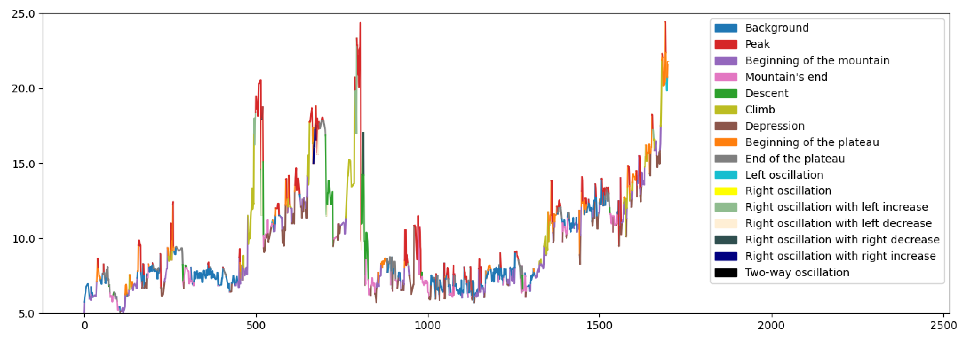
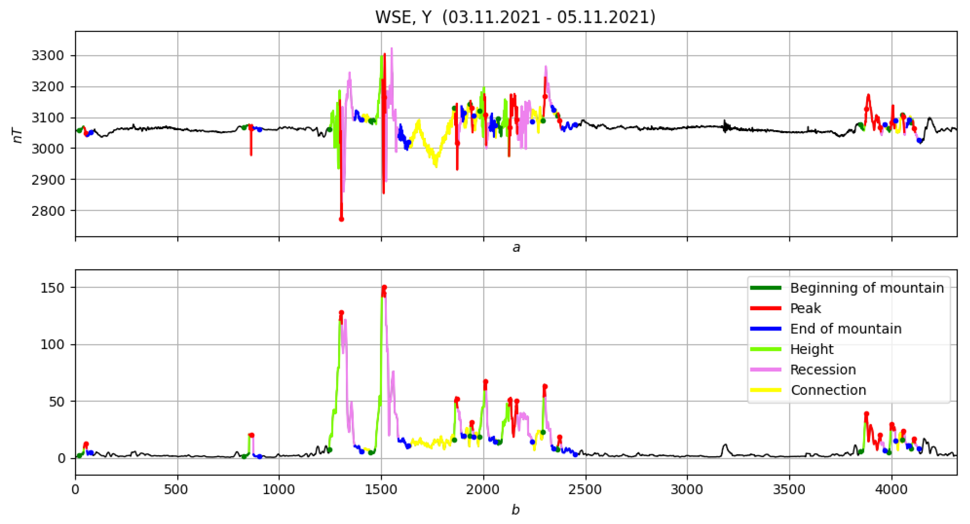
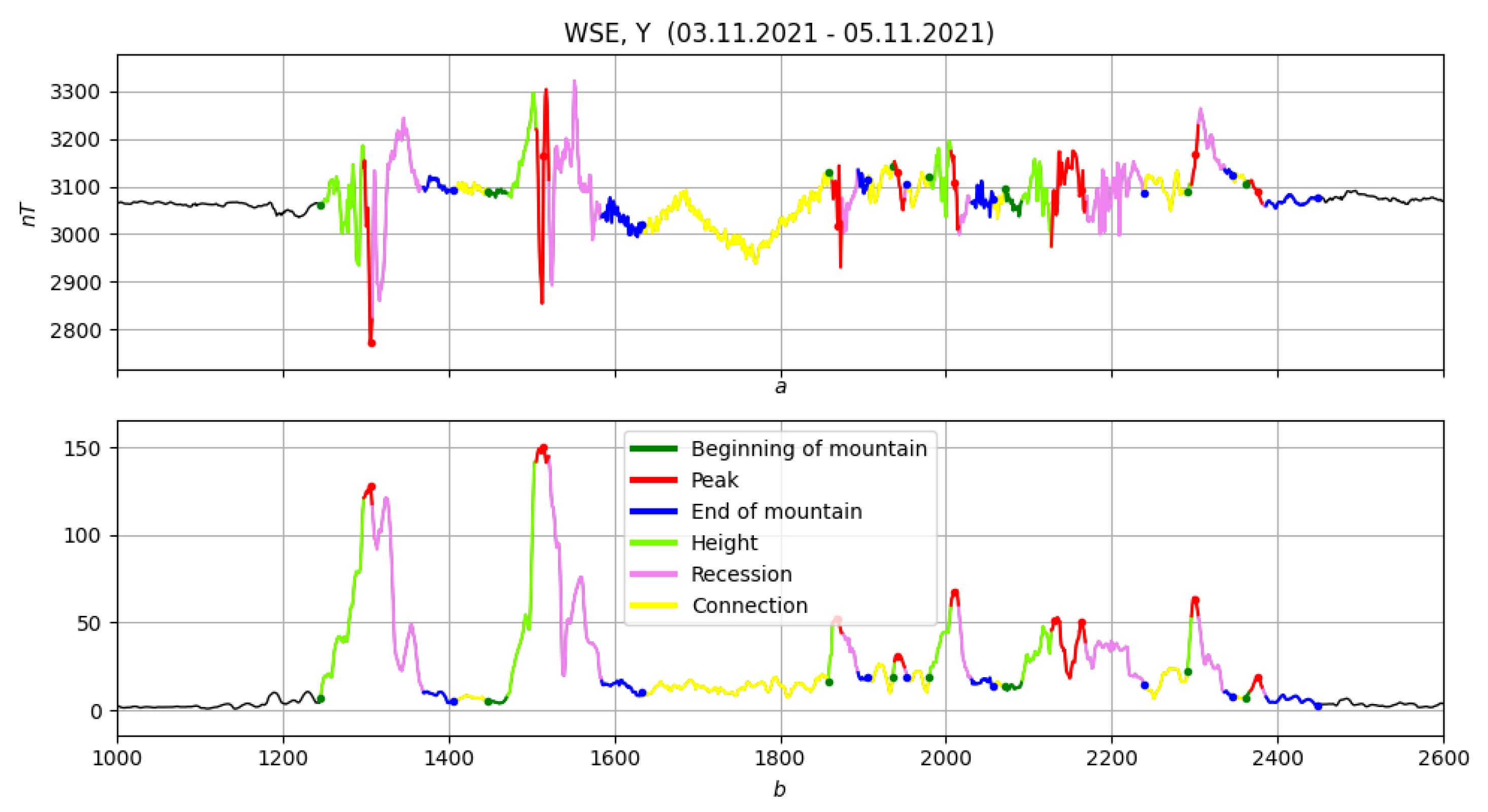
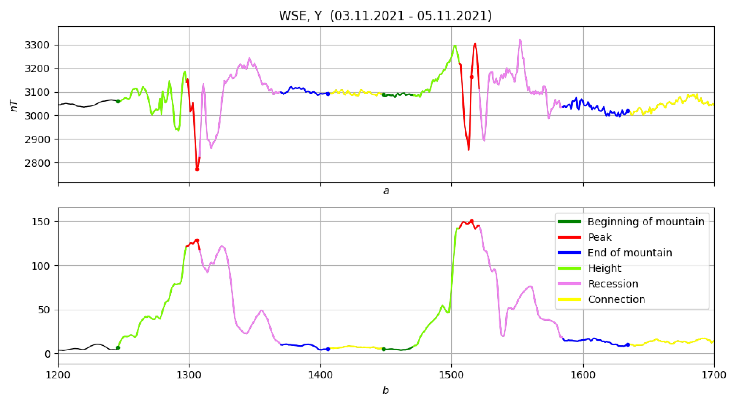
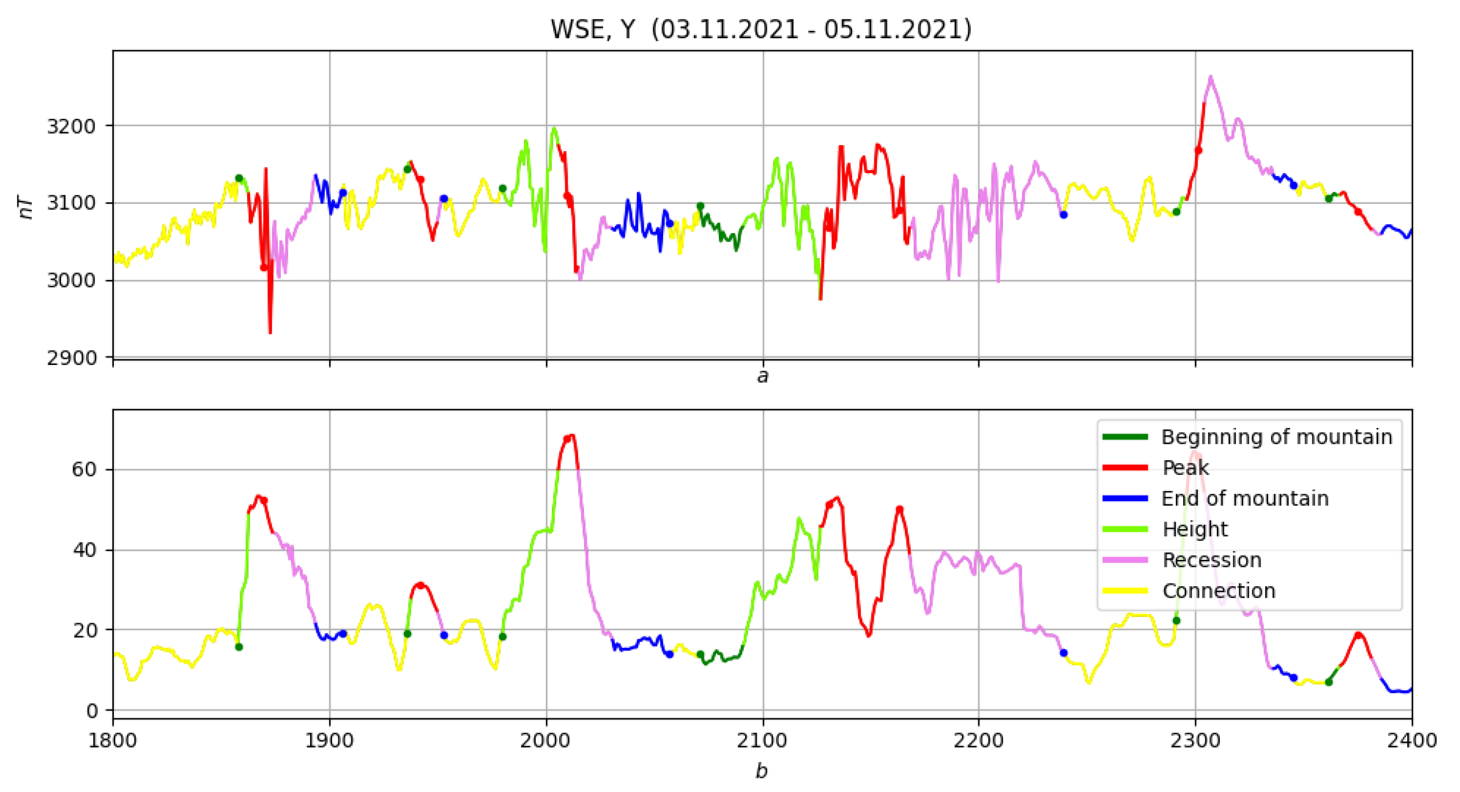
4.3. Example: Morphological Analysis of a Magnetic Storm Record
Conclusions
5. Conclusions
Author Contributions
Funding
Informed Consent Statement
Acknowledgments
Conflicts of Interest
Abbreviations
| DMA | Discrete Mathematical Analysis |
| FM | Fuzzy Mathematics |
| FL | Fuzzy Logic |
| DRAS | Difference Recognition Algorithm for Signals |
| FCARS | Fuzzy Comparison Algorithm for Recognition of Signals |
| MAGNUS | Monitoring and Analysis of Geomagnetic aNomalies in Unified System |
References
- Gvishiani, A.; Soloviev, A. Observations, Modeling and Systems Analysis in Geomagnetic Data Interpretation; Springer International Publishing: Cham, Switzerland, 2020. [Google Scholar] [CrossRef]
- Agayan, S.M.; Bogoutdinov, S.R.; Krasnoperov, R.I. Short introduction into DMA. Russ. J. Earth Sci. 2018, 18, 1–10. [Google Scholar] [CrossRef]
- Gvishiani, A.D.; Agayan, S.M.; Bogoutdinov, S.R.; Zlotnicki, J.; Bonnin, J. Mathematical methods of geoinformatics. III. Fuzzy comparisons and recognition of anomalies in time series. Cybern. Syst. Anal. 2008, 44, 309–323. [Google Scholar] [CrossRef]
- Gvishiani, A.D.; Agayan, S.M.; Bogoutdinov, S.R. Fuzzy recognition of anomalies in time series. Dokl. Earth Sci. 2008, 421, 838–842. [Google Scholar] [CrossRef]
- Agayan, S.; Bogoutdinov, S.; Soloviev, A.; Sidorov, R. The Study of Time Series Using the DMA Methods and Geophysical Applications. Data Sci. J. 2016, 15, 16. [Google Scholar] [CrossRef]
- Serra, J. Image Analysis and Mathematical Morphology; Academic Press: Cambridge, MA, USA, 1982; p. 610. [Google Scholar]
- Serra, J. Image Analysis and Mathematical Morphology, Volume 2: Theoretical Advances, 1st ed.; Academic Press: Cambridge, MA, USA, 1988; p. 411. [Google Scholar]
- Matheron, G. Random Sets and Integral Geometry; Wiley: New York, NY, USA, 1975; p. 261. [Google Scholar]
- Gonzalez, R.C.; Woods, R.E. Digital Image Processing, 4th ed.; Pearson: London, UK, 2017; p. 1192. [Google Scholar]
- Maragos, P. Pattern spectrum and multiscale shape representation. IEEE Trans. Pattern Anal. Mach. Intell. 1989, 11, 701–716. [Google Scholar] [CrossRef]
- Urbach, E.R.; Roerdink, J.; Michael Wilkinson, M.H.F. Connected Shape-Size Pattern Spectra for Rotation and Scale-Invariant Classification of Gray-Scale Images. IEEE Trans. Pattern Anal. Mach. Intell. 2007, 29, 272–285. [Google Scholar] [CrossRef] [PubMed]
- Wilkinson, M.H.F. Generalized pattern spectra sensitive to spatial information. In Proceedings of the 16th International Conference on Pattern Recognition, Québec City, QC, Canada, 11–15 August 2002; Volume 1, pp. 21–24. [Google Scholar] [CrossRef]
- Kulichkov, S.N.; Chulichkov, A.I.; Demin, D.S. Morphological Analysis Infrasonic Signals in Acoustics; Novyi Akropol: Moscow, Russia, 2010; p. 132. (In Russian) [Google Scholar]
- Pyt’ev, Y.; Chulichkov, A. Morphological Methods for Image Analysis; Fiz-matlit Publisher: Moscow, Russia, 2010; p. 336. (In Russian) [Google Scholar]
- Pyt’ev, Y. Morphological image analysis. Pattern Recognit. Image Anal. 1993, 3, 19–28. (In Russian) [Google Scholar]
- Vizil’ter, Y.V.; Zheltov, S.Y.; Bondarenko, A.V.; Osokov, M.V.; Morzhin, A.V. Image Processing and Analysis in Machine Vision Problems. A Course of Lectures and Practical Exercises; Fizmatkniga: Moscow, Russia, 2010; p. 672. (In Russian) [Google Scholar]
- Zadeh, L.A. The Concept of a Linguistic Variable and its Application to Approximate Reasoning. In Learning Systems and Intelligent Robots; Springer: New York, NY, USA, 1974; pp. 1–10. [Google Scholar] [CrossRef]
- Novák, V.; Perfilieva, I.; Močkoř, J. Mathematical Principles of Fuzzy Logic; Springer: New York, NY, USA, 1999. [Google Scholar] [CrossRef]
- Box, G.E.P.; Jenkins, G.M. Time Series Analysis: Forecasting and Control; Holden-Day: San Francisco, CA, USA, 1976. [Google Scholar]
- Hamilton, J.D. Time Series Analysis; Princeton University Press: Princeton, NJ, USA, 1994. [Google Scholar] [CrossRef]
- Priestley, M.B. Spectral Analysis and Time Series; Academic Press Inc.: New York, NY, USA, 1981. [Google Scholar]
- Shumway, R.H.; Stoffer, D.S. Time Series Analysis and Its Applications; Springer International Publishing: Cham, Switzerland, 2017. [Google Scholar] [CrossRef]
- Woodward, W.A.; Gray, H.L.; Elliot, A.C. Applied Time Series Analysis; CRC Press: Boca Baton, FL, USA, 2012. [Google Scholar]
- Chen, S.M. Forecasting enrollments based on fuzzy time series. Fuzzy Sets Syst. 1996, 81, 311–319. [Google Scholar] [CrossRef]
- Novák, V.; Perfilieva, I.; Dvořák, A. Insight into Fuzzy Modeling; John Wiley & Sons, Inc.: New York, NY, USA, 2016. [Google Scholar] [CrossRef]
- Song, Q.; Chissom, B.S. Fuzzy time series and its models. Fuzzy Sets Syst. 1993, 54, 269–277. [Google Scholar] [CrossRef]


Disclaimer/Publisher’s Note: The statements, opinions and data contained in all publications are solely those of the individual author(s) and contributor(s) and not of MDPI and/or the editor(s). MDPI and/or the editor(s) disclaim responsibility for any injury to people or property resulting from any ideas, methods, instructions or products referred to in the content. |
© 2023 by the authors. Licensee MDPI, Basel, Switzerland. This article is an open access article distributed under the terms and conditions of the Creative Commons Attribution (CC BY) license (https://creativecommons.org/licenses/by/4.0/).
Share and Cite
Agayan, S.M.; Kamaev, D.A.; Bogoutdinov, S.R.; Aleksanyan, A.O.; Dzeranov, B.V. Time Series Analysis by Fuzzy Logic Methods. Algorithms 2023, 16, 238. https://doi.org/10.3390/a16050238
Agayan SM, Kamaev DA, Bogoutdinov SR, Aleksanyan AO, Dzeranov BV. Time Series Analysis by Fuzzy Logic Methods. Algorithms. 2023; 16(5):238. https://doi.org/10.3390/a16050238
Chicago/Turabian StyleAgayan, Sergey M., Dmitriy A. Kamaev, Shamil R. Bogoutdinov, Andron O. Aleksanyan, and Boris V. Dzeranov. 2023. "Time Series Analysis by Fuzzy Logic Methods" Algorithms 16, no. 5: 238. https://doi.org/10.3390/a16050238
APA StyleAgayan, S. M., Kamaev, D. A., Bogoutdinov, S. R., Aleksanyan, A. O., & Dzeranov, B. V. (2023). Time Series Analysis by Fuzzy Logic Methods. Algorithms, 16(5), 238. https://doi.org/10.3390/a16050238