Abstract
Chest X-ray image classification suffers from the high inter-similarity in appearance that is vulnerable to noisy labels. The data-dependent and heteroscedastic characteristic label noise make chest X-ray image classification more challenging. To address this problem, in this paper, we first revisit the heteroscedastic modeling (HM) for image classification with noise labels. Rather than modeling all images in one fell swoop as in HM, we instead propose a novel framework that considers the noisy and clean samples separately for chest X-ray image classification. The proposed framework consists of a Gaussian Mixture Model-based noise detector and a Heteroscedastic Modeling-based noise-aware classification network, named GMM-HM. The noise detector is constructed to judge whether one sample is clean or noisy. The noise-aware classification network models the noisy and clean samples with heteroscedastic and homoscedastic hypotheses, respectively. Through building the correlations between the corrupted noisy samples, the GMM-HM is much more robust than HM, which uses only the homoscedastic hypothesis. Compared with HM, we show consistent improvements on the ChestX-ray2017 dataset with different levels of symmetric and asymmetric noise. Furthermore, we also conduct experiments on a real asymmetric noisy dataset, ChestX-ray14. The experimental results on ChestX-ray14 show the superiority of the proposed method.
1. Introduction
The chest X-ray is one of the most common examination methods to diagnose thorax diseases in medical screening. In practice, the diagnosis system needs a large amount of accurately labeled data to train a deep model. Manually distinguishing different pathologies in screening is a time-consuming and labor-intensive task. Moreover, a large number of noisy labels are also easily introduced in the annotations of chest X-ray images. First, chest X-rays caused by different causative agents usually present similarities in appearance, which make it difficult to distinguish. Furthermore, the noisy labels could also originate from other kinds of factors, e.g., inter-observer variability, annotation errors, or errors generated by the annotation algorithms. Therefore, it is important to explore a robust, accurate, computer-aided diagnosis system with noisy labels to assist in diagnosing radiographs.
Chest X-ray image classification suffers from specific heteroscedastic and highly data-dependent noise. Figure 1a–c show different kinds of pneumonia and the normal case of chest X-ray images. Pneumonia (caused by bacteria or a virus) images, even the normal images, show very high inter-similarity in appearance. Compared with the noise existing in natural images, the highly noisy labels in chest X-ray image datasets often happen in the related classes. Furthermore, chest X-ray image classification is also limited by the high similarity in the feature space. In Figure 1d, we visualize the features extracted by ResNet-50 [1] with the t-distributed stochastic neighbor embedding (t-SNE). The manifolds of bacterial and viral pneumonia and normal samples locate very close; thus, they are difficult to correctly classify with the network.
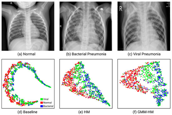
Figure 1.
Examples of (a) Normal, (b) Bacterial Pneumonia, (c) Viral Pneumonia, and (d–f) are the visualized t-SNE feature distributions of the Baseline, HM, and the proposed GMM-HM methods (with 20% asymmetric noise on the ChestX-ray2017 dataset [2]).
Collier et al. [3] propose heteroscedastic modeling (HM) that places a multivariate normally distributed latent variable on the final hidden layer of a neural network classifier for the heteroscedastic label noise. HM breaks the homoscedasticity assumptions in network optimization with a cross-entropy loss function. However, for most of the existing datasets, only parts of the samples are wrongly annotated. Modeling all the samples with the relaxed hypothesis, especially the large number of clean samples, would affect the network convergence and increase the burden of network optimization. In Figure 1e, we could observe that the distance between the normal and the pneumonia is expanded with HM. However, the bacterial and viral pneumonia samples still locate very close and are difficult to recognize. Therefore, to enhance efficiency, it is necessary to handle the clean and noisy samples individually.
In this paper, rather than model all the samples in one fell swoop as in [3], we propose to consider the clean and noisy samples separately and construct a novel framework that integrates noise detection and noise-aware classification for chest X-ray image classification with noisy labels. The noise detection module builds on a Gaussian Mixture Model (GMM) to judge whether one sample is clean or noisy. The noise-aware classification network consists of two branches that extract the specific features for clean and noisy samples and classify the input images. For the clean samples, we input them into the backbone network and classify them as usual, while for the noisy samples, we add a heteroscedastic layer to model the aleatoric uncertainty due to the data-dependent label noise. As shown in Figure 1f, by introducing noise detection and HM, the feature distribution of different kinds of samples is much easier to distinguish compared with that of HM. We verify the effectiveness of the proposed method by conducting extensive experiments on a pediatric pneumonia dataset (very easily introducing noise), ChestX-ray2017, and a real noisy dataset, ChestX-ray14. Empirically, GMM-HM is superior to HM in recognition performance.
We summarize the contributions of this work as follows:
- We revisit Heteroscedastic Modeling and illustrate that it is superior for modeling the clean and noisy samples separately, rather than modeling all images in one fell swoop for chest X-ray image classification with noisy labels.
- We propose a novel GMM-HM that integrates a GMM-based noise detector and an HM-based noise-aware classification into a unified framework to classify the chest X-ray images with noisy labels.
- We present a superior performance improvement on both the ChestX-ray2017 and the ChestX-ray14 datasets. The proposed GMM-HM shows strongly superior performance compared with the baseline and HM methods on symmetric and asymmetric noise on the ChestX-ray2017 dataset. On the ChestX-ray14 dataset, GMM-HM also achieves comparable or even better performance than the state-of-the-art methods.
Table 1 gives details of the abbreviations in this paper.

Table 1.
The abbreviation table.
2. Related Works
2.1. Chest X-ray Image Classification with Noisy Labels
Chest X-ray (CXR) image classification with deep learning has been widely explored and achieved significant progress in recent years. Some methods focus on generating more discriminative features to facilitate classification by designing novel architectures in deep neural networks [4,5,6,7,8,9,10]. Some other methods use the attention mechanism to improve the classification performance by focusing on the lesion area, e.g., [11,12,13,14,15,16]. In addition, some methods try to improve classification performance by capturing dependencies between chest disease labels [17,18,19].
Label noise is inevitably introduced into the large-scale chest X-ray image dataset due to the errors produced by the annotators or the annotation algorithms. The deep networks are easily overfitted to these noisy samples, which leads to performance degradation. To combat the noise in medical images, Karimi et al. [20] investigate the probabilistic methods against label noise in solving medical image analysis tasks. Pham et al. [21] use the label smoothing regularization (LSR) technique [22] to handle noisy samples. Calli et al. [23] propose to use model confidence and uncertainty as metrics to identify samples mislabeled as emphysema in the chest X-ray images. Chen et al. [24] propose to correct the label noise by building an attribute-level graph and estimating the virtual attributes of CXR images. Li et al. [25] propose a Bootstrap Knowledge Distillation (BKD) method to correct noisy labels and theoretically deduce that the distribution of distilled labels is closer to the ground truth. Liu et al. [26] use an improved Early Learning Regularization (ELR) [27] loss function to robustly combat noise. Gundel et al. [28] design a noise-resistant loss function that takes the human-assessed label noise probability and the observed label correlation as two priors for the loss functions. Xue et al. [29] propose a collaborative training framework to filter and train clean samples. Some methods also use a self-supervised learning strategy for noisy samples and design a loss function to mitigate overfitting to noisy labels in global and local representation learning for CXR images.
Most of the existing methods aim at designing robust loss functions or designing efficient strategies to identify the noise labels and then correct them. Unlike previous works, we consider the label noise from the aspect of label generation and design a robust model to combat noise for chest X-ray image classification.
2.2. Heteroscedastic Classification
Kendall et al. [30] propose to model the heteroscedasticity between the pixels among the boundaries by placing a Gaussian distribution with diagonal covariance matrix over the network outputs in the semantic segmentation task. The study in [30] could be considered as a special case of the method of [31]. Collier et al. [31] perform general heteroscedastic modeling (HM) that assumes the noise term is a multivariate normal distribution. HM computes an input-dependent covariance matrix which enables modeling the inter-class label noise correlations on a per-image basis. Experiments show that HM can effectively improve image classification and segmentation performance under input-dependent label noise. The chest X-ray images with noisy labels exhibit heteroscedasticity which is data-dependent. In this paper, we explore the heteroscedasticity classification in chest X-ray images. Unlike [3], we illustrate that it is superior to separate the clean and noisy samples and model them individually. Therefore, we propose a novel framework that includes a noise detector and a noise-aware classification module to achieve the above purpose.
3. Methodology
3.1. Revisiting Heteroscedastic Modeling
Heteroscedastic-based methods have been explored to model label noise, offering an objective method for image classification with data-dependent label noise. Collier et al. [3] propose to model such noise based on probabilistic modeling [30,31]. Suppose there are some latent vectors of utility , where C is the number of classes. The utility is the sum of a deterministic reference utility and a stochastic component , . The label of input image x is generated by sampling from the utility and taking the argmax, i.e., an image belongs to class c if its associated utility is greater than the utility for all other classes,
where C is the number of the classes. Conventionally, the popularly used cross-entropy loss function in training a neural network is precisely the closed-form solution of predictive probabilities under the assumption that the stochastic component is the Gumbel distribution independently,
Meanwhile, the Gumbel noise distribution is always too restrictive for the data-dependent label noise. Collier et al. [3] propose to break the above assumption by assuming that the noise term is a multivariate normal distribution, . To solve the problem of no closed-form solution, the Monte Carlo estimation is used to approximate the expectation of . Notice that the gradient-based optimization would be infeasible; thus, the is approximated with a temperature-parameterized ,
where S is the number of Monte Carlo samplings.
3.2. The Proposed GMM-HM
3.2.1. Overview of the Framework
The framework of GMM-HM is shown in Figure 2. GMM-HM consists of a Gaussian Mixture Model-based noise detector and a Heteroscedastic Modeling-based noise-aware classification network. During training, we build a GMM on the sample loss values in the previous epoch to divide the samples into a clean set and a noisy set in each epoch. The clean and noisy samples are input to the corresponding clean or noisy branch in the noise-aware classification network. The noisy branch models the data-dependent noisy samples with a heteroscedastic layer. Then, the clean or noisy samples are classified. The two branches share the weights of the backbone. The network is optimized with a cross-entropy loss function. During testing, all the samples are fed into the clean branch to be classified.
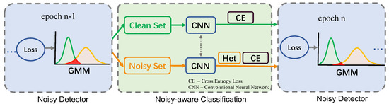
Figure 2.
The framework of the proposed GMM-HM.
3.2.2. Noisy Detector
Generally, the small-loss samples are considered as the clean ones, and the large-loss samples as the noisy ones [32,33]. We could straightforwardly use the loss values to distinguish the clean and the noisy samples by setting a threshold. However, the threshold is difficult to choose for different datasets. Another way is to model the loss distribution and then distinguish the clean or noisy samples by the distribution. Li et al. [33] propose that due to the flexibility of the Gaussian Mixture Model (GMM) model distribution, clean and noise samples can be better distinguished. To this end, we build a GMM based on the losses to determine whether one sample is clean or noisy.
Given training data , where N is the total number of training images, is the i-th training image and is its label vector. C is the number of the pathologies. If belongs to class c, then ; otherwise, . Let be the loss values at the epoch of producing the best performance. We build a K-component GMM to loss values , and the predicted probability of each sample is formalized as
where and are the mean and standard variance of the k-th Gaussian component, respectively. is the weight of the k-th Gaussian component. K is 2 in our experiments. The parameters , , and of the GMM can be estimated using the Expectation Maximization algorithm. At each epoch, GMM divides the training data into a clean set and a noisy set. Specifically, we distinguish one sample as belonging to clean set () or noisy set () by setting a threshold T on the ,
where g is the Gaussian component with a smaller mean (small loss). Generally, we set the T as 0.5 in the experiment. At the first epoch, due to the fact that there are effective loss values, we consider all the training samples as clean ones, feeding into the clean branch of the noise-aware classification network. In subsequent training, we dynamically fit a two-component GMM on its per-sample loss distribution in the previous epoch to divide the training samples into a noisy and a clean set. Whether a sample belongs to the clean or noisy set is determined by the posterior probability whose loss belongs to the Gaussian component with smaller mean (smaller loss). That is, if is larger than a threshold T, the corresponding sample is judged to the clean set. Otherwise, it would be classified as noisy. Therefore, all the samples in the noisy set would input into the noisy branch of the noise-aware classification network from the second epoch in the training.
3.2.3. Noisy-Aware Classification
The noise-aware classification network consists of two branches for dealing with the clean and noisy samples, respectively. The clean branch is as same as the classical classification networks, e.g., ResNet [1]. The noisy branch is placed in a multivariate normally distributed latent variable on the final hidden layer of the classifier. The clean and noisy branches share the weights of the CNN backbone. The clean and noisy samples are fed into the corresponding branches to be classified.
Let the predicted logits of an image x as , where f represents the deep networks with parameter . We omit the subscript of x for simplification. Next, to make a clear distinction in this section, we denote the samples coming from clean set and noisy set as and , respectively. The predicted logits of clean samples are directly input into the classifier. The logits of noisy samples are first fed into the heteroscedastic layer to compute the heteroscedastic representation , which is then fed into the final classifier.
The is computed as follows. We compute the deterministic item as , where and are the parameters of a convolutional layer. The stochastic item of the heteroscedastic layer is implemented with a low-rank approximation method by , where is a matrix, and . In practice, the is computed as an affine transformation of as , where and are the parameters of a convolutional layer. In order to ensure the positive semi-definiteness of the covariance matrix, a C-dimensional vector is added to the diagonal of ,
where is a diagonal correction matrix. and are the parameters of a convolutional layer. and are sampled from and , respectively. ⊙ denotes the element-wise multiplication. Finally, the latent vector of input is computed by
3.2.4. Optimization
Algorithm 1 shows the whole training procedures. Let g denote the classifier of the neural network with parameters . We denote the predicted logits representing the output logits of x. With , we optimize the deep network by measuring the classification loss.
The classification loss is computed by cross-entropy or binary cross-entropy loss functions determined by the tasks. For the multi-class classification task, the probability is obtained by feeding the logits into the Softmax function . The loss is calculated with a cross-entropy loss function as follows,
For the multi-label classification task, the probability is calculated with the Sigmoid function . Then the network is optimized by the binary cross-entropy loss function,
| Algorithm 1: The trainingprocedures of the proposed GMM-HM |
Input: Training dataset , threshold T Initialization: Weights [, ] 1 while epoch < MaxEpoch do 2 // construct the GMM based on the loss values in the previous epoch. 3 4 5 if 6 //inputting the clean branch. 7 else 8 //inputting the noisy branch, and computing the latent vector as Equation (7) 10 updating with SGD. 11 end |
4. Experiment
This section evaluates the performance of the proposed GMM-HM. We first introduce the experimental datasets, evaluation metrics, and training details in Section 4.1 and Section 4.2, respectively. Then, we compare and analyze the performance of the GMM-HM on different datasets in Section 4.3. Finally, we also visualize the features to demonstrate the effectiveness of the proposed method.
4.1. Datasets and Evaluation Metrics
ChestX-ray2017 [2] has a total of 5856 anterior-posterior Chest X-ray images. Each CXR image belongs to either normal, bacterial pneumonia, or viral pneumonia. The training and testing sets include 5232 and 624 images, respectively. On ChestX-ray2017, we conduct experiments with symmetric and asymmetric noise following previous works [33,34]. ChestX-ray2017 is a clean dataset. We artificially add 20%, 40%, and 60% symmetric or asymmetric noise on the training set, respectively. Symmetric noise means that any class of labels is replaced by any class. Asymmetric noise means that label swapping occurs only for similar categories. We compute the Accuracy (Acc), Sensitivity (Sens), Specificity (Spec), and AUC as the evaluation of the proposed method,
where TP, FP, FN, and TN are true positive, false positive, false negative, and true negative, respectively. AUC (Area Under The Curve) is the area under the ROC (Receiver Operating Characteristics) curve.
ChestX-ray14 [4] contains a total of 112,120 frontal-view chest X-ray images of 30,805 patients. ChestX-ray14 is a real asymmetric noisy dataset whose noise labels originate from algorithm errors. The noise proportion of the training set and test set is unknown. This dataset includes 14 pathologies: Atelectasis, Cardiomegaly, Effusion, Infiltration, Mass, Nodule, Pneumonia, Pneumothorax, Consolidation, Edema, Emphysema, Fibrosis, PT, and Hernia. The training set and validation set have 86,524 images, and the test set has 25,596 images. The AUC score for each pathology and the average AUC over 14 pathologies are used to evaluate the performance of the proposed method.
4.2. Implementation Details
First, we introduce the details about how GMM is applied. In one training epoch, we fit a two-component GMM on the per-sample loss in the previous epoch to divide the training samples into a noisy and a clean set. The posterior probability of one sample whose loss belongs to the Gaussian component with a smaller mean larger than T (0.5 in the experiments) belongs to the clean set. Otherwise, it belongs to the noisy set. Second, for the noise-aware network, we perform data augmentation by randomly resizing and cropping to 224 × 224 and randomly horizontal flipping and normalizing with the mean and standard variance of ImageNet [34] in training. During testing, the image is also resized to 224 × 224. We train the GMM-HM with a stochastic gradient descent algorithm with an initial learning rate of 0.01. The batch size is set to 16. The threshold T in GMM is set to 0.5. On the ChestX-ray14 dataset, we train the network using stochastic gradient descent with an initial learning rate of 0.01. The learning rate is reduced by a factor of 10 after every 30 epochs. The batch size is 64. In HM and GMM-HM for both of these two datasets, we set the momentum to 0.9 and weight decay to 5e-4 in SGD, the softmax temperature to 1.5, and MC samples to 10,000.
4.3. Comparative Studies
Comparitive Methods. (1) Baseline.We train a ResNet-50 [1] as our baseline method. We replace the last fully connected layer with a C-dimensional fully connected layer to classify the input images, e.g., on ChestX-ray2017 and on ChestX-ray14. (2) Heteroscedastic Modeling. We also compare our method to the original Heteroscedastic Modeling (HM) [3]. In HM, we input all the samples into the heteroscedastic layer and do not distinguish the clean or noisy samples like our proposed GMM-HM.
4.3.1. Results on ChestX-ray2017
Table 2 shows the results on the ChestX-ray2017 dataset. We train a strong baseline on the ChestX-ray2017 dataset with different levels of symmetric or asymmetric noise. We first analyze the symmetric noise case. When the noise level is 20%, the accuracy of the Baseline is 84.29%, the sensitivity is 84.29%, the specificity is 91.95%, and the AUC is 93.60%. By introducing the Heteroscedastic Modeling of noise labels, these four evaluation metrics are obviously improved, especially the accuracy and sensitivity (about 2%). Promoted by our GMM-HM, the performance over all the evaluation metrics is further enhanced by at least 1%. Compared with the Baseline, GMM-HM achieves a significant improvement of about 3% in accuracy and sensitivity. When the noise level increases to 40%, the entire performance of the Baseline method decreases by about 2%. We observe that the improvement with HM is slight on some metrics, e.g., specificity and AUC. On the other metrics, the performance is improved by about 1%. However, GMM-HM is not affected by the noise ratio and promotes performance improvement on all metrics by about 3%. We could obtain similar or greater improvements when the noise ratio increases to 60%. Particularly, compared with Baseline, the AUC of GMM-HM achieves a significant improvement of about 4.29%.
Table 2.
The experimental results on the ChestX-ray2017 dataset.
Next, we analyze the case where the noise type is asymmetric noise. When the noise ratio is 20%, the accuracy of the Baseline is 84.94%, the sensitivity is 84.94%, the specificity is 91.96%, and the AUC is 94.46%. Similar to the symmetric noise, the performance on the four evaluation metrics is improved by introducing the Heteroscedastic Modeling for noisy samples. We could observe that the performance of most of these metrics is enhanced by over 2%, e.g., accuracy and sensitivity. The proposed GMM-HM obtains greater performance gains on all evaluation metrics, especially the sensitivity with 3.36%. When the noise ratio increases to 40%, we could observe that the performance with HM and GMM-HM is consistently improved by about 1–2%. Particularly, GMM-HM significantly improves the accuracy and sensitivity by 2.4%. With a larger 60% asymmetric noise, the pneumonia recognition performance largely decreases with the Baseline method. The HM introduces about 1–2% improvement on the four evaluation metrics. Particularly, HM surpasses the Baseline by about 5% on the AUC score. With GMM-HM, we observe that the pneumonia recognition performance is tremendously enhanced compared with the Baseline method, e.g., AUC with 7.63%, accuracy and sensitivity with about 5%. We empirically conclude that the data-independent pneumonia noise is properly modeled by the HM and separating the noise and clean samples could also benefit further performance enhancement.
4.3.2. Results on ChestX-ray14
Table 3 reports the AUC score of each pathology and the average AUC score of 14 pathologies of Baseline, HM, and GMM-HM methods on the ChestX-ray14 dataset. We train a relatively strong baseline which achieves an average AUC of 0.805. By introducing the heteroscedastic modeling for the noisy samples, the average AUC score of 14 pathologies achieves 0.812. We observe that the AUC scores of “Emphysema” and “Hernia” are obviously improved from 0.893 to 0.904 and 0.885 to 0.915, respectively. This illustrates that introducing the noise label strategy could benefit the model performance on the chestX-ray14 dataset. While further handling the noisy and clean samples separately, the proposed GMM-HM achieves the highest average AUC score of 0.822 among the three methods. Moreover, among the 14 pathologies, some of them are improved significantly, e.g., over 2% for “Pneumonia”, “Pneumothorax”, and “Hernia”. The results suggest that detecting noisy samples and modeling the noisy data with a heteroscedastic layer is necessary to robustly combat noise and improve classification performance. In Table 3, we also report the performance comparisons with the state-of-the-art methods.
Table 3.
Comparisons of GMM-HM with Baseline and HM methods on ChestX-ray14.
Previous works focus on network design and performance improvement but seldom consider the noisy labels existing in ChestX-ray14. By considering the data-correlated noise, GMM-HM performs better than other methods. The average AUC score achieves 0.822, which is better than the SOTA [28]. Among the 14 pathologies, GMM-HM surpasses other methods by a large gap and has the best AUC score on the “Hernia” (0.945). In addition, on “Infiltration”, “Pneumonia”, “Pneumothorax”, and “Edema”, the AUC score of GMM-HM also achieves a new state of the art. Basically, the proposed GMM-HM achieves comparable or even better performance compared with the state-of-the-art methods.
4.3.3. Feature Visualization
Figure 3 visualizes the features of the Baseline, HM, and GMM-HM methods with t-SNE [36] on different datasets. On the ChestX-ray2017 dataset, with the Baseline method, shown in Figure 1d, pneumonia and normal samples locate very close, which makes them difficult to distinguish. With HM, the distances between pneumonia and normal samples become larger, but the bacterial and viral pneumonia samples are still difficult to correctly classify (Figure 1e). With GMM-HM, we observe that the features of normal and pneumonia, even the bacterial and viral pneumonia samples, are further separated, which leads to easy classification (Figure 1f). As shown in Table 2 and Table 3, GMM-HM also exceeds the HM and Baseline methods by a large gap and benefits from better feature representation. On the ChestX-ray14 dataset, as shown in Figure 3, we randomly select two pathologies to show the feature distributions and could also conclude that the proposed GMM-HM is superior to the HM and the Baseline methods.
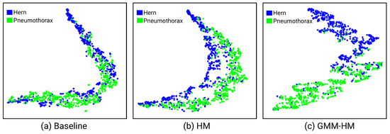
Figure 3.
(a–c) are the visualized t-SNE feature distributions of the Baseline, HM, and the proposed GMM-HM methods on the ChestXray14 dataset.
5. Conclusions
In this paper, we rethink heteroscedastic modeling for chest X-ray image classification with noisy labels. Rather than inputting all the samples into the heteroscedastic layer, we propose a novel framework that considers the clean and noisy samples separately. A GMM-based noise detector and an HM-based noise-aware classification are integrated into a framework to robustly detect noisy samples and correctly classify the input images. Experimental results demonstrate the superiority of the proposed framework for pneumonia classification and multi-label disease classification tasks. In the future, instead of imposing a classification step between clean and noisy, we would consider keeping the conditional probabilities of the GMM and integrating them into the classification decision under a Bayesian approach framework.
Author Contributions
Q.G. and Q.C. (Formal analysis, Validation, Writing-Review, Editing, Experiments, Draft writing), Y.H. (Supervision, Writing-Review). All authors have read and agreed to the published version of the manuscript.
Funding
The research was funded by China Postdoctoral Science Foundation (2022M710338) and the Fundamental Research Funds for the Central Universities (2022JBMC008).
Data Availability Statement
The data used in this article are publicly available at ChestX-ray2017 (https://www.kaggle.com/paultimothymooney/chest-xray-pneumonia, accessed on 1 March 2023) and ChestX-ray14 (https://nihcc.app.box.com/v/ChestXray-NIHCC, accessed on 1 March 2023).
Conflicts of Interest
The authors declare no conflict of interest.
References
- He, K.; Zhang, X.; Ren, S.; Sun, J. Deep residual learning for image recognition. In Proceedings of the IEEE Conference on Computer Vision and Pattern Recognition, Las Vegas, NV, USA, 27–30 June 2016; pp. 770–778. [Google Scholar]
- Kermany, D.S.; Goldbaum, M.; Cai, W.; Valentim, C.C.; Liang, H.; Baxter, S.L.; McKeown, A.; Yang, G.; Wu, X.; Yan, F.; et al. Identifying medical diagnoses and treatable diseases by image-based deep learning. Cell 2018, 172, 1122–1131. [Google Scholar] [CrossRef]
- Collier, M.; Mustafa, B.; Kokiopoulou, E.; Jenatton, R.; Berent, J. Correlated input-dependent label noise in large-scale image classification. In Proceedings of the IEEE/CVF Conference on Computer Vision and Pattern Recognition, Nashville, TN, USA, 20–25 June 2021; pp. 1551–1560. [Google Scholar]
- Wang, X.; Peng, Y.; Lu, L.; Lu, Z.; Bagheri, M.; Summers, R.M. Chestx-ray8: Hospital-scale chest x-ray database and benchmarks on weakly-supervised classification and localization of common thorax diseases. In Proceedings of the IEEE Conference on Computer Vision and Pattern Recognition, Honolulu, HI, USA, 21–26 July 2017; pp. 2097–2106. [Google Scholar]
- Shen, Y.; Gao, M. Dynamic routing on deep neural network for thoracic disease classification and sensitive area localization. In Proceedings of the International Workshop on Machine Learning in Medical Imaging, Granada, Spain, 16 September 2018; Springer: Cham, Switzerland, 2018; pp. 389–397. [Google Scholar]
- Chen, B.; Li, J.; Guo, X.; Lu, G. DualCheXNet: Dual asymmetric feature learning for thoracic disease classification in chest X-rays. Biomed. Signal Process. Control 2019, 53, 101554. [Google Scholar] [CrossRef]
- Guan, Q.; Huang, Y.; Luo, Y.; Liu, P.; Xu, M.; Yang, Y. Discriminative Feature Learning for Thorax Disease Classification in Chest X-ray Images. IEEE Trans. Image Process. 2021, 30, 2476–2487. [Google Scholar] [CrossRef]
- Wang, X.; Peng, Y.; Lu, L.; Lu, Z.; Summers, R.M. Tienet: Text-image embedding network for common thorax disease classification and reporting in chest x-rays. In Proceedings of the IEEE Conference on Computer Vision and Pattern Recognition, Salt Lake City, UT, USA, 18–22 June 2018; pp. 9049–9058. [Google Scholar]
- Bhatt, C.M.; Patel, P.; Ghetia, T.; Mazzeo, P.L. Effective Heart Disease Prediction Using Machine Learning Techniques. Algorithms 2023, 16, 88. [Google Scholar] [CrossRef]
- Alamr, A.; Artoli, A. Unsupervised Transformer-Based Anomaly Detection in ECG Signals. Algorithms 2023, 16, 152. [Google Scholar] [CrossRef]
- Ypsilantis, P.P.; Montana, G. Learning what to look in chest X-rays with a recurrent visual attention model. arXiv 2017, arXiv:1701.06452. [Google Scholar]
- Tang, Y.; Wang, X.; Harrison, A.P.; Lu, L.; Xiao, J.; Summers, R.M. Attention-guided curriculum learning for weakly supervised classification and localization of thoracic diseases on chest radiographs. In Proceedings of the International Workshop on Machine Learning in Medical Imaging, Granada, Spain, 16 September 2018; Springer: Cham, Switzerland, 2018; pp. 249–258. [Google Scholar]
- Chen, B.; Li, J.; Lu, G.; Zhang, D. Lesion location attention guided network for multi-label thoracic disease classification in chest X-rays. IEEE J. Biomed. Health Inform. 2019, 24, 2016–2027. [Google Scholar] [CrossRef]
- Guan, Q.; Huang, Y. Multi-label chest X-ray image classification via category-wise residual attention learning. Pattern Recognit. Lett. 2020, 130, 259–266. [Google Scholar] [CrossRef]
- Ma, C.; Wang, H.; Hoi, S.C. Multi-label thoracic disease image classification with cross-attention networks. In Proceedings of the International Conference on Medical Image Computing and Computer-Assisted Intervention, Shenzhen, China, 13–17 October 2019; Springer: Cham, Switzerland, 2019; pp. 730–738. [Google Scholar]
- Lei, K.; Syed, A.; Zhu, X.; Pauly, J.; Vasanawala, S. Automated MRI Field of View Prescription from Region of Interest Prediction by Intra-Stack Attention Neural Network. Bioengineering 2023, 10, 92. [Google Scholar] [PubMed]
- Yao, L.; Poblenz, E.; Dagunts, D.; Covington, B.; Bernard, D.; Lyman, K. Learning to diagnose from scratch by exploiting dependencies among labels. arXiv 2017, arXiv:1710.10501. [Google Scholar]
- Kumar, P.; Grewal, M.; Srivastava, M.M. Boosted cascaded convnets for multilabel classification of thoracic diseases in chest radiographs. In Proceedings of the International Conference Image Analysis and Recognition, Póvoa de Varzim, Portugal, 27–29 June 2018; Springer: Cham, Switzerland, 2018; pp. 546–552. [Google Scholar]
- Chen, B.; Li, J.; Lu, G.; Yu, H.; Zhang, D. Label co-occurrence learning with graph convolutional networks for multi-label chest x-ray image classification. IEEE J. Biomed. Health Inform. 2020, 24, 2292–2302. [Google Scholar] [CrossRef]
- Karimi, D.; Dou, H.; Warfield, S.K.; Gholipour, A. Deep learning with noisy labels: Exploring techniques and remedies in medical image analysis. Med. Image Anal. 2020, 65, 101759. [Google Scholar] [CrossRef] [PubMed]
- Pham, H.H.; Le, T.T.; Tran, D.Q.; Ngo, D.T.; Nguyen, H.Q. Interpreting chest X-rays via CNNs that exploit hierarchical disease dependencies and uncertainty labels. Neurocomputing 2021, 437, 186–194. [Google Scholar] [CrossRef]
- Müller, R.; Kornblith, S.; Hinton, G.E. When does label smoothing help? Adv. Neural Inf. Process. Syst. 2019, 32, 6448–6458. [Google Scholar]
- Calli, E.; Sogancioglu, E.; Scholten, E.T.; Murphy, K.; van Ginneken, B. Handling label noise through model confidence and uncertainty: Application to chest radiograph classification. In Proceedings of the Medical Imaging 2019: Computer-Aided Diagnosis, San Diego, CA, USA, 17–20 February 2019; SPIE: Washington, DC, USA, 2019; Volume 10950, pp. 289–296. [Google Scholar]
- Chen, Y.; Liu, F.; Tian, Y.; Liu, Y.; Carneiro, G. Semantic-guided Image Virtual Attribute Learning for Noisy Multi-label Chest X-ray Classification. arXiv 2022, arXiv:2203.01937. [Google Scholar]
- Li, M.; Xu, J. Bootstrap Knowledge Distillation for Chest X-ray Image Classification with Noisy Labelling. In Proceedings of the International Conference on Image and Graphics, Haikou, China, 26–28 December 2021; Springer: Cham, Switzerland, 2021; pp. 704–715. [Google Scholar]
- Liu, F.; Tian, Y.; Cordeiro, F.R.; Belagiannis, V.; Reid, I.; Carneiro, G. Noisy label learning for large-scale medical image classification. arXiv 2021, arXiv:2103.04053. [Google Scholar]
- Liu, S.; Niles-Weed, J.; Razavian, N.; Fernandez-Granda, C. Early-learning regularization prevents memorization of noisy labels. Adv. Neural Inf. Process. Syst. 2020, 33, 20331–20342. [Google Scholar]
- Gündel, S.; Setio, A.A.; Ghesu, F.C.; Grbic, S.; Georgescu, B.; Maier, A.; Comaniciu, D. Robust classification from noisy labels: Integrating additional knowledge for chest radiography abnormality assessment. Med. Image Anal. 2021, 72, 102087. [Google Scholar] [CrossRef]
- Xue, C.; Yu, L.; Chen, P.; Dou, Q.; Heng, P.A. Robust Medical Image Classification from Noisy Labeled Data with Global and Local Representation Guided Co-training. IEEE Trans. Med. Imaging 2022, 41, 1371–1382. [Google Scholar] [CrossRef]
- Kendall, A.; Gal, Y. What uncertainties do we need in bayesian deep learning for computer vision? Adv. Neural Inf. Process. Syst. 2017, 30, 1–11. [Google Scholar]
- Collier, M.; Mustafa, B.; Kokiopoulou, E.; Jenatton, R.; Berent, J. A simple probabilistic method for deep classification under input-dependent label noise. arXiv 2020, arXiv:2003.06778. [Google Scholar]
- Han, B.; Yao, Q.; Yu, X.; Niu, G.; Xu, M.; Hu, W.; Tsang, I.; Sugiyama, M. Co-teaching: Robust training of deep neural networks with extremely noisy labels. Adv. Neural Inf. Process. Syst. 2018, 31, 1–11. [Google Scholar]
- Li, J.; Socher, R.; Hoi, S.C. DivideMix: Learning with Noisy Labels as Semi-supervised Learning. In Proceedings of the International Conference on Learning Representations, New Orleans, LA, USA, 6–9 May 2019. [Google Scholar]
- Russakovsky, O.; Deng, J.; Su, H.; Krause, J.; Satheesh, S.; Ma, S.; Huang, Z.; Karpathy, A.; Khosla, A.; Bernstein, M.; et al. Imagenet large scale visual recognition challenge. Int. J. Comput. Vis. 2015, 115, 211–252. [Google Scholar] [CrossRef]
- Guendel, S.; Grbic, S.; Georgescu, B.; Liu, S.; Maier, A.; Comaniciu, D. Learning to recognize abnormalities in chest x-rays with location-aware dense networks. In Proceedings of the Iberoamerican Congress on Pattern Recognition, Madrid, Spain, 19–22 November 2018; Springer: Cham, Switzerland; pp. 757–765. [Google Scholar]
- Van der Maaten, L.; Hinton, G. Visualizing data using t-SNE. J. Mach. Learn. Res. 2008, 9, 2579–2605. [Google Scholar]
Disclaimer/Publisher’s Note: The statements, opinions and data contained in all publications are solely those of the individual author(s) and contributor(s) and not of MDPI and/or the editor(s). MDPI and/or the editor(s) disclaim responsibility for any injury to people or property resulting from any ideas, methods, instructions or products referred to in the content. |
© 2023 by the authors. Licensee MDPI, Basel, Switzerland. This article is an open access article distributed under the terms and conditions of the Creative Commons Attribution (CC BY) license (https://creativecommons.org/licenses/by/4.0/).