Article

Quantum Circuit-Width Reduction through Parameterisation and Specialisation

1
School of Computing Science, University of Glasgow, Glasgow G12 8QQ, UK
2
James Watt School of Engineering, University of Glasgow, Glasgow G12 8QQ, UK
*
Author to whom correspondence should be addressed.
Algorithms 2023, 16(5), 241; https://doi.org/10.3390/a16050241
Submission received: 27 February 2023 / Revised: 17 April 2023 / Accepted: 21 April 2023 / Published: 5 May 2023
(This article belongs to the Special Issue Space-Efficient Algorithms and Data Structures)

Abstract

:
As quantum computing technology continues to develop, the need for research into novel quantum algorithms is growing. However, such algorithms cannot yet be reliably tested on actual quantum hardware, which is still limited in several ways, including qubit coherence times, connectivity, and available qubits. To facilitate the development of novel algorithms despite this, simulators on classical computing systems are used to verify the correctness of an algorithm, and study its behaviour under different error models. In general, this involves operating on a memory space that grows exponentially with the number of qubits. In this work, we introduce quantum circuit transformations that allow for the construction of parameterised circuits for quantum algorithms. The parameterised circuits are in an ideal form to be processed by quantum compilation tools, such that the circuit can be partially evaluated prior to simulation, and a smaller specialised circuit can be constructed by eliminating fixed input qubits. We show significant reduction in the number of qubits for various quantum arithmetic circuits. Divide-by-n-bits quantum integer dividers are used as an example demonstration. It is shown that the complexity reduces from 4 n + 2 to 3 n + 2 qubits in the specialised versions. For quantum algorithms involving divide-by-8 arithmetic operations, a reduction by 2 8 = 256 in required memory is achieved for classical simulation, reducing the memory required from 137 GB to 0.53 GB.

1. Introduction

In recent years, research in Quantum Computing (QC) [1] has developed into a large-scale global activity aimed at creating ever more capable quantum computing hardware, as well as quantum computing applications, with the potential to revolutionise computational science. Despite this progress, current and near-future quantum computers (commonly referred to as Noisy Intermediate-Scale Quantum (NISQ)-era quantum computers [2]) are still limited in their capability. Realising the potential of quantum computers requires that certain features of quantum mechanics not available in classical computing are exploited. The potential computational benefit of quantum computers relies on information being processed while encoded in a coherent quantum state in the qubit register. In NISQ-era hardware, information is encoded in a relatively small number of qubits, with limited connectivity between qubits and a limited extent of quantum error correction techniques. Quantum error correction is needed to maintain this coherent state for a sufficiently long time so that meaningful computations can be performed. Recently, quantum computers with O ( 100 ) `noisy’ qubits (e.g., prone to significant quantum errors and decoherence) have been realised [3]. This is projected to grow to O ( 10 4 ) or O ( 10 5 ) [4] in the coming decade. This way, future quantum hardware with more fault-tolerance can be built, where the quantum error correction is used on the many implemented qubits to create O ( 100 ) fault-tolerant or `functional qubits’ (as termed by IBM).
In addition to the challenges involved in realising quantum hardware, it is also clear that major challenges exist in devising suitable applications and algorithms for quantum computers. Theoretical aspects of quantum algorithms, as well as the implementation in terms of quantum circuits represent major research areas.
A key role in developing quantum algorithms and their realisation on quantum hardware is played by quantum computing simulation on classical computing hardware. Applications requiring a number of qubits not yet available on hardware can be evaluated provided sufficient classical computing resources are available. This type of simulation also allows to evaluate for example the performance and reliability of an algorithm in the presence of simulated quantum errors.
As reviewed later this section, the representation in a classical simulation of a coherent quantum state involving n qubits in its most general form requires 2 n degrees of freedom. This characteristic forms a key aspect of the huge potential of quantum computers (“exponential speed-ups”). At the same time, it means that even for relatively small quantum computer applications, the classical computing resources required for simulation become excessive. For illustration, the Intel Quantum Simulator [5] was demonstrated recently for simulations using 42 qubits on a state-of-the-art supercomputing facility.
Reducing the computational cost of simulating quantum circuits on classical hardware forms the main motivation of the present investigation. Specifically, the present work introduces transformations to quantum algorithms represented in terms of a quantum circuit, leading to more compact representations involving fewer qubits and, thus, reduced storage needs for the simulation.
Quantum circuit transformation methods represent a broad and active research area. One type of transformations map quantum circuits to specific quantum hardware. In the quantum circuit model (detailed later), quantum algorithms can be expressed in terms of quantum gate operations, such that all qubits can access all other qubits. For more limited connectivity in specific hardware configurations, a transformation of the circuit representation is then required. Childs et al. [6] present a recent review of such transformations. Another type of transformations, closer related to the present work, involves circuit transformation aimed at facilitating classical simulation on large-scale distributed memory computing facilities. Graph-based transformation techniques have been introduced by a range of researchers to achieve a reduction in memory requirements. Boixo et al. [7], Chen et al. [8], and Schutski et al. [9] employ a tensor network-based approach, while Pednault et al. [10] use an undirected graph model. Further transformation methods presented in the literature include the circuit partitioning scheme described by Chen et al. [11] and the implicit decomposition technique described by Li et al. [12], transforming the original circuit into multiple, smaller transformed circuits so that communication in parallel simulations on classical computers could be reduced.
The quantum circuit transformations introduced in this work are mainly aimed at facilitating simulating quantum circuits on classical computers. Additionally, the introduced transformation can be used in quantum hardware realisations, where the qubit count reduction can be used to facilitate realisation of circuits that would not fit without the transformations introduced here. It is important to note that the output of the proposed transformation involves gate operations with multiple control qubits (as detailed later). Therefore, a subsequent transpilation step accounting for available native gates and qubit connectivity of target quantum hardware is required for quantum hardware realisations. For quantum circuit simulation on classical hardware, a similar transpilation step is often required for applications where the impact of (modelled) quantum gate errors is investigated. In the transpilation step, a well-considered trade-off between quantum circuit width and quantum circuit depth is required to avoid undoing the circuit width reduction achieved by the quantum circuit transformations introduced here. If IBM quantum hardware is used in realisation, the transformation step in IBM Qiskit [13] would be performed after the transformations proposed here. Beyond IBM’s Qiskit, several other tools exist that were designed to facilitate the specification and transformation of quantum circuits, e.g., Quipper [14], OpenQASM 3 [15,16], Xanadu’s Strawberry Fields [17], PennyLane [18], and Microsoft Q# [19]. Xanadu’s tools primarily focus on Quantum Machine Learning and compilation to photonic quantum computers; OpenQASM is an effort to standardise quantum circuit specification. While the circuit specification and manipulation techniques provided by Qiskit, Quipper, and Microsoft Q# are similar to those provided by our toolchain, these tools were developed for more general circuit transformations and do not provide a similar functionality in terms of static analysis to achieve circuit width reduction of parameterised quantum arithmetic circuits.
The transformations introduced in this work rely on the concept of identifying qubits in the circuit that can be specialised to a constant value, i.e., | 0 or | 1 , as explained later. If the identified qubit only acts as control qubit in the quantum gate operations in the circuit, then two independent circuits (with one fewer qubit) can be defined for both choices of the specialised qubit. This approach works independent of the application domain for which the considered quantum circuit was developed, and was used in a different context in the works on circuit partitioning [11] and circuit decomposition [12], as mentioned previously. The second concept on which the transformations introduced in this work rely involves exploiting application domain knowledge to facilitate the identification of qubits suitable for specialisation. As explained later in this section, a wide range of practically important quantum algorithms exist where quantum arithmetic occurs as part of the larger computation. This includes the famous Shor algorithm for integer factorization [20]. In typical quantum circuit implementations of arithmetic operations, the identification of qubits suitable for the specialisation outlined above is a challenging task as a result of qubits acting repeatedly as control, as well as target qubit in gate operations. However, in reversible arithmetic operations, half of the input qubits will have an unchanged state upon completion of the computation. This domain-specific feature motivated the development of transformations of arithmetic circuits to a parameterised form such that qubit specialisation can be automated in a quantum computing toolchain. This second aspect of the introduced quantum circuit transformations involving parameterisation of circuits represents the main novelty of the present work. Despite this use of domain specific knowledge, it is shown that the approach is still general enough for a wide range of quantum algorithms in the field of computational science and engineering.
In a broader context, it can be noted that program transformation algorithms are essential constituents of modern compilers for classical languages [21,22,23,24]. These are used to optimise the instructions corresponding to the original source code of a program to, e.g., minimise register use, instruction count or run time, or make optimal use of features, such as vector operations. Thus, the current work can be considered as extending the concept of program transformations to the field of quantum computing. The specific transformations presented are quantum circuit substitutions that allow static analysis tools to easily specialise circuits for fixed inputs, reducing the quantum circuit width (qubit count).
Our main motivation for reducing the number of required qubits is to reduce the classical computing resources. However, the introduced transformations can also be used to create smaller circuits for proof-of-concept demonstrations on near-future quantum hardware, and would be an integral part of any future compiler for mature quantum computers.
The rest of this section presents a brief review of quantum computing concepts, provides context in terms of the type of quantum algorithms our transformations introduced are aimed at, and presents the primary contributions of this work.

1.1. Brief Review of Quantum Computing Essentials

In this section, some core concepts of quantum computing that are particularly relevant to this work are reviewed. A full treatment can be found in [1].

1.1.1. Qubit Representation and Manipulation

In quantum computing, qubits are the units of information that can be manipulated. Using the Dirac notation, a single qubit can be described by two complex probability amplitudes
| q = a | 0 + b | 1 ; | a | 2 + | b | 2 = 1
such that | a | 2 is the probability of finding the qubit in state | 0 and | b | 2 is the probability of finding the qubit in state | 1 . We can compose a system with two qubits by taking the tensor product of the qubits’ state vectors
| q 0 | q 1 = | q 0 | q 1 = a 0 a 1 | 00 + a 0 b 1 | 01 + b 0 a 1 | 10 + b 0 b 1 | 11
showing that in this case 4 complex amplitudes define the quantum state | q 0 | q 1 where | 00 , | 01 , | 10 , and | 11 represent the four computational basis states. This concept can be extended to n qubits, such that the quantum wave function, | Ψ is defined by 2 n complex amplitudes
| Ψ = k = 0 2 n 1 C k | k
where | k represent the 2 n computational basis states, with the integer value of k obtained from the binary representation of the n qubits. Another way of interpreting this is that a system of n qubits forms a 2 n -dimensional Hilbert space. In quantum mechanics, operations performed on the quantum state are represented by unitary Hermitian matrices. In the quantum circuit model, discussed in next section, these unitary operations are performed by quantum gates.

1.1.2. Quantum Circuit Model

The quantum circuit model is widely used in Quantum Computing to represent quantum algorithms as a series of “quantum gate” operations acting on one or more qubits. Each of the qubits is represented by a horizontal solid line in quantum circuit diagrams, with a vertical arrangement of the multiple qubits in the register. The number of qubits and, therefore, the number of parallel lines defines the circuit width. Quantum gates are designed to either work on a single qubit (“single-qubit gates”) or work on multiple qubits simultaneously (“multi-qubit gates”). The quantum computation progresses step-by-step in the horizontal direction, starting from the initial qubit register state defined on the left-hand side. The diagram in the left-hand side of Figure 1 shows a simple two-qubit quantum circuit with a single two-qubit gate acting on the state of qubits | q 1 | q 0 . The example shows a controlled- N O T ( C N O T ) operation, where the N O T (also termed X in quantum computing) is performed on qubit | q 0 conditional on qubit | q 1 = | 1 . This operation represent a single time instance. The X gate ( X 0 1 1 0 ) has the effect of flipping a qubit in the computational basis, such that X | 0 = | 1 , X | 1 = | 0 , by swapping of the qubit’s probability amplitudes. This is the analogue of the classical NOT gate. In more complex circuits, a series of such quantum gate operations is performed step-by-step. For illustration, the right-hand side of Figure 1 shows how a general single-qubit gate G with a negative control (here | q 1 = | 0 ) can be implemented using a sequence of three gate operations. The number of time slices required to run the circuit (i.e., circuit slices with gates that affect mutually exclusive qubits) defines the circuit depth. Since a quantum circuit is composed of unitary operations, every quantum circuit has an inverse. The inverse of a quantum circuit can simply be composed of the inverse of all its constituent quantum gates, applied in reverse order. The operation of applying the inverse of a circuit after “moving” useful data from the circuit is common in quantum computing, and is termed uncomputation. This is typically used to return qubits allocated to create workspace to their initial state, so that these can be re-used in subsequent parts of the circuit.
The quantum circuits considered in the current work typically involve tens or hundreds of qubits, with a quantum circuit depth of tens to thousands of gate operation steps. Simulating quantum circuits with this number of qubits clearly represents a major computational challenge.

1.2. Context of Present Work

In recent years, significant research efforts have focused on developing quantum algorithms for computational engineering applications, including fluid dynamics, with the aim of achieving significant quantum speed-up. A promising line of investigation in the context of computational fluid dynamics focuses on developing quantum circuit implementations of lattice-based models of a range of problems [25,26,27,28,29,30,31]. A quantum algorithm for the collisionless Boltzmann equation and its application to rarefied supersonic flows was presented by Todorova and Steijl [25,26]. Budinski [27] introduced a quantum algorithm for the linear advection–diffusion equation based on the Lattice Boltzmann method. In this work and in the work of Todorova and Steijl [25], particle distribution functions defined in each of the lattice sites on the considered regular lattice move to a neighbouring site during subsequent time steps. The quantum circuit implementation of this step shows strong similarity with quantum modulo adders. Therefore, it can be expected that the transformations introduced here can also be extended to this type of circuits. In the Lattice Boltzmann method, a collision term appears on the right-hand side of the equation and its non-linearity for the Navier–Stokes equations in fluid dynamics was considered by Steijl [29] using quantum floating-point arithmetic and using Carleman linearisation in the work of Itani and Succi [28]. In the context of the Lattice Boltzmann method for fluid dynamics, in Moawad et al. [30] the authors presented quantum circuit implementations of non-linear one-dimensional models. More recently, the quantum circuit implementation of multi-dimensional non-linear lattice models was presented by one of the authors [31]. Both these works employed an application-specific floating-point representation with reduced precision relative to the IEEE-754 single-precision standard [32]. A key feature of this ongoing work on quantum circuit implementation of lattice modelling is the reliance on a range of quantum arithmetic operations. An illustrative example is shown in Figure 2 where for a fixed-point definition of velocities u and v in a two-dimensional problem, the quantity u 2 + v 2 (i.e., directly related to kinetic energy) is evaluated using a shift-and-add based approach to sum contributions from u and v into the output register defining u 2 + v 2 . The quantum circuit shown in Figure 2 is based on the more complex circuits shown in Steijl [31] that involve floating-point operations. For the current work, the modified 4-qubit full adders F A u and F A v are of particular interest. Specifically, for larger fixed-point data representations with an increased number of qubits, it is clear that the quantum circuit width often exceeds the size that can be routinely simulated using a full state vector Quantum Circuit Simulator (as discussed in more detail in Section 3). In the ongoing development of quantum algorithms for lattice-based modeling, but also many further quantum algorithms employing similar quantum arithmetic operations, the quantum circuit width is often a limiting factor. This means that for quantum algorithms involving quantum arithmetic operations, the introduction of circuit-width reduction steps on the circuit performing quantum arithmetic operations would facilitate the classical simulation of larger circuits, as well as a wider range of quantum algorithms.

1.3. Exemplar Circuit: Integer Divider

Figure 3 shows a top-level representation of a quantum integer divider as an illustrative example and as the target application in this work. The design shown performs a 4-step long division to create a 4-qubit quotient | o u t 3 | o u t 2 | o u t 1 | o u t 0 from a dividend defined by a 7-qubit register and a divisor defined by a 4-qubit register | q 3 d | q 2 d | q 1 d | q 0 d . The 7-qubit dividend register comprises the original 4-qubit representation of the dividend | q 3 i | q 2 i | q 1 i | q 0 i extended by three qubits in state | 0 , i.e., | q i n 2 | q i n 1 | q i n 0 . This integer divider can for example be used in fixed-point arithmetic, or as part of a floating-point divider. The key building blocks of this quantum circuit are the Comparator (indicated by C in Figure 3) and its uncomputation (termed U ( C ) in Figure 3), as well as the controlled Subtractor operations. As can be seen, once the 4-qubit register | o u t 3 | o u t 2 | o u t 1 | o u t 0 is defined, the controlled subtractions are uncomputed using controlled add ( A d d in Figure 3) circuits to restore all qubits to their original state, except the four qubits defining desired output. Possible quantum circuit implementations of these operations are detailed in Figure 4, where the comparator is based on the subtractor circuits proposed by Xia et al. [33].
The design and quantum circuit implementation of quantum comparators has been investigated in detail in the past decade [33,34,35,36]. Often, this work was conducted in the context of quantum image processing, where the comparator circuits were employed in image binarisation. The circuits take as input two multi-qubit registers defining integers a and b in binary representation. For use in quantum long-division only a < b or a b need to be identified, while some of the comparator designs also separate a = b and a > b . The work of Xia et al. al. [33] includes a brief review of past work on quantum comparators. The type of quantum comparator circuits introduced by Xia et al. [33] is well-suited to the requirements of the present work since it involves a minimum number of auxiliary qubits. It was also recently used in the work of Yuan et al. [37], where the design of a fault-tolerant implementation of quantum divider was considered.
It should be noted that the quantum circuit transformation steps demonstrated here using the quantum integer divider target a wider range of quantum arithmetic operations and should, therefore, benefit a significant research community working on quantum arithmetic circuits and their application within more complex algorithms. From the quantum computing literature, it is clear that work on quantum arithmetic circuits remains an active area of research, even after two decades of work. Relating to the example shown in Figure 2 for a quantum circuit used for evaluation of kinetic energy in fixed-point representation in a two-dimensional lattice-based model, work on the development of efficient quantum multipliers constitutes significant ongoing activity [38,39,40]. Recent work on improved quantum circuits for addition and subtraction often focuses on fault-tolerant implementations, e.g., Orts et al. [41] propose three fault-tolerant carry look-ahead adders that improve the cost in terms of quantum gates and qubits relative to previous works. Recently, a quantum circuit design for single-precision floating-point division was presented by Gayathri et al. [42]. Their emphasis was on creating resource estimates in terms of number of qubits required, as well as circuit depth. This type of research work could benefit from the quantum circuit transformation introduced here as it facilitates more efficient classical simulations of the circuits.

1.4. Contributions of This Work

The main novelty and contributions of the presented work can be summarized as follows:
  • Demonstration of quantum circuit width reduction transformations based on Circuit Parameterisation and Qubit Specialisation for quantum algorithms performing arithmetic operations as part of the computational work;
  • Demonstration of the derivation steps used in creating parameterised quantum circuits for quantum arithmetic. The formulation in parameterised form for a quantum comparator and a quantum subtractor are detailed. To the best of the authors’ knowledge, these parameterised circuits have not been considered in the literature before. The derivations detailed here also show how similar parameterisation can be applied to a wider range of arithmetic circuits;
  • Analysis of the quantum circuit design of integer dividers in terms of suitability for the proposed quantum circuit width transformations;
  • Demonstration how for the quantum divider exemplar the pre-computed and verified comparator and subtractor circuits in parameterised form can be imported into the complete quantum circuit implementation, followed by the automated selection of qubits suitable for specialisation and the automated specialisation for different user-defined inputs;
  • Analysis in terms of circuit complexity of specialised quantum integer divider circuits as obtained from the transformation techniques introduced. The correctness of the circuits is verified using a quantum circuit simulator.
The rest of this manuscript is structured as follows. Section 2 presents the two main types of data encoding techniques used in quantum information processing. Section 3 discusses key aspects of simulation of quantum circuits on a classical computer. The key concepts introduced in this work are outlined in Section 4. Section 5 describes the derivation of the parameterised comparator and its specialised forms. Section 6 then details the parameterised subtractor circuits. Section 7 describes the design and quantum circuit implementation of quantum integer dividers. The quantum circuit toolchain employed in this work is described in Section 8. Section 9 demonstrates the implementation of the divider in the presented toolchain and describes its specialisation and verification. The results of using the toolchain to reduce the divider are presented. Finally, Section 10 presents the conclusions and suggestions for future work.

2. Data Encoding in Quantum Information

The quantum circuit transformation approaches introduced here were designed to reduce quantum circuits performing quantum arithmetic operations. In the intended application, the quantum circuit considered represents a larger, and more general quantum algorithm were the arithmetic represents a part of the computational work. Quantum arithmetic operations typically rely on a specific type of data encoding. To explain this further, the two main data encoding approaches used in quantum information processing are summarized here.
In amplitude-based encoding, a vector of normalised complex data (of size up to N = 2 n ) is encoded into the amplitudes, C k in Equation (3). This encoding technique is the most widely used encoding technique in quantum algorithms since it creates the most direct means of taking advantage of quantum parallelism (i.e., exponential growth of number of degrees of freedom with linear increase in the number of qubits). For this type of data encoding, the most widely used quantum circuit simulation approach on classical computers is full state vector simulation, where the 2 n complex amplitudes are all stored and the gate operations in a considered circuit lead to step-by-step modifications of these amplitudes.
In the present work, the focus is on the alternative approach termed computational-basis encoding. In this data encoding approach, the quantum algorithm is designed such that at initialisation only the complex amplitude of a single computational basis state has non-zero amplitude. After completion of the quantum algorithm the output is represented similarly by a single non-zero amplitude for one of the quantum basis states. For quantum algorithms employing the computational basis encoding a few important observations relevant to the present work can be made:
  • The motivation for this type of encoding is typically performing quantum arithmetic operations;
  • To maintain the property that only a single computational basis state has a non-zero amplitude throughout the computation, the gates in the Quantum Circuit model are limited to quantum equivalents of logic gates (e.g., X as equivalent of N O T and Toffoli as doubly-controlled N O T ). By doing so, the quantum circuit can efficiently be simulated on a classical computer using a logic-based simulator. In such a simulator, n classical bits suffice to represent the state of n qubits. Then, the controlled logic gate operations conditionally flip states between 0 and 1;
  • If quantum arithmetic operations are implemented in the quantum circuit model based on the Quantum Fourier Transform [43,44], then efficient simulation using classical logic-based simulation is not possible, since the QFT in the case of quantum arithmetic circuits temporarily moves the encoding approach to amplitude-based encoding, before finally returning an output in computational basis encoding.
Since the circuit transformation approaches introduced here target quantum arithmetic operations, key aspects of computational basis encoding were used in creating these transformation steps. Specifically, identifying qubits that throughout a quantum computation are guaranteed to remain in either state | 0 or | 1 relies on this type of encoding throughout the computation or at least for the considered part of the algorithm performing arithmetic operations. For more general algorithms using amplitude encoding the transformation approaches introduced cannot be employed.
Relating to the use of the transformation approaches in quantum algorithm development process, the following observations need to be made:
  • The quantum arithmetic operations in circuit using computational basis encoding considered here can be efficiently simulated on a classical computer using a logic based simulator—these circuits act as classical reversible circuits when not used as part of a larger quantum algorithm;
  • As arithmetic blocks which operate in the computational basis are often parts of larger quantum algorithms, quantum circuit simulations often require a full-state vector simulation approach;
  • For quantum circuit simulations where the effect of (modeled) quantum errors are included, the full-state vector simulation approach is generally required even for algorithms operating entirely (through computation) with computational basis encoding.
Because of the essential role played by full-state vector simulation, this aspect of quantum algorithm analysis is considered in more detail in the following section.

3. Quantum Circuit Simulation

In this section, the full-state vector simulation of quantum circuits is considered in more detail. As mentioned in Section 1.1, the quantum state of n qubits in a qubit register is defined by 2 n complex amplitudes defining the quantum wave function. In a full-state vector quantum circuit simulator, the 2 n complex numbers are all stored in memory irrespective of the amplitude. Specifically, in cases where many of the amplitudes are zero, the potential savings offered by only storing non-zero amplitudes are not employed. During the evolution of the quantum state in the considered quantum computation, some or even all amplitudes will change in time, complicating approaches where only non-zero amplitudes are stored.
In general, to simulate the operation of a quantum gate on a full state vector, the entire memory space needs to be accessed. The access pattern depends on the index of the gate’s target qubit in the quantum register. This index t is 0 for the least significant qubit in the indexing used (at the bottom of quantum circuit diagrams), while t = n 1 for the most significant qubit (at the top of quantum circuit diagrams). The memory space is accessed in pairs, where the stride between the pair elements is 2 t , for target t. Each pair is then updated by direct matrix-vector multiplication by the gate’s 2 × 2 matrix. As an example of the computational work involved in quantum circuit simulation, consider the application of a general gate, G = a b c d , where a , b , c , d C , on the most-significant qubit. If the initial quantum state is defined by | Ψ 0 and the state after applying the gate by | Ψ 1 then
| Ψ 1 = k = 0 2 n C k ( 1 ) | k
where complex amplitudes C k ( 1 ) are related to previous amplitudes C k ( 0 ) as
C k ( 1 ) = a C k ( 0 ) + b C k + 2 t ( 0 ) C k + 2 t ( 1 ) = c C k ( 0 ) + d C k + 2 t ( 0 )
for k [ 0 , 2 n 1 1 ] . The indexing of the amplitudes in Equation (5) shows that the simulation of gate operations in the quantum circuit model typically involves large memory strides. For the application of a gate on the qubit that represents the most-significant bit in terms of indexing, this stride equals half the state-vector length, i.e., 2 n 1 . In an application of a gate on the qubit representing the least-significant bit in the indexing, the stride in memory reduces to 1.

4. Discussion of Key Concepts

A key aspect of the quantum circuit transformations presented in this work involves reducing the number of qubits by redefining the circuit for specific states of one or more qubits. To illustrate this concept, consider the reduction of a 3-qubit modulo adder. Figure 5 illustrates the step-by-step specialisation of the ripple-carry 3-qubit modulo adder for the specific case | a 2 | a 1 | a 0 = | 101 . In terms of 2’s complement representation, this modulo adder can then be used to subtract 3 from a positive integer represented in binary by 2 qubits | b 1 | b 0 . In the modulo adder, this input is set as | b 2 | b 1 | b 0 with | b 2 = | 0 .
In Figure 5, ‘Step 0’ shows the Cuccaro-type modulo adder [45] with the M A J (Majority) and U M A (UnMajority and Add) blocks expanded. The 3-qubit modulo adder in its unmodified form employs three M A J blocks on the left-hand side of the circuit shown, and three U M A blocks on the right-hand side. The steps shown in the figure are described here:
  • Step 1: For the three most-significant qubits | a 2 | r 2 | a 1 at the top of the circuit, the gate operations in the neighbouring M A J and U M A blocks partially cancel out. Specifically, only two C N O T s remain. The C N O T with | a 2 as control and | b 2 target can then be reduced to a N O T on | b 2 since in the specialisation shown | a 2 = | 1 .
  • Step 2: | a 1 = | 0 is accounted for by removing the three C N O T s where | a 1 acts as control.
  • Step 3: The actions on | a 1 can be removed by replacing the two Toffoli gates that conditionally change | a 1 = | 0 into state | 1 and the C N O T gate with | b 2 as target, by a single Toffoli gate with | b 2 as target and with the same control qubits as the replaced Toffoli gates.
  • Step 4: | a 0 = | 1 is accounted for first by replacing three C N O T s by three N O T s.
  • Step 5: The three N O T s resulting from the previous step are then accounted for by modifying the control in two Toffoli gates with | a 0 as target.
  • Step 6: | c = | 0 is accounted for by removing | c as control from the two Toffoli gates with | b 0 as target and removing the C N O T with | b 0 as target.
  • Step 7: The actions on | a 0 are removed by removing the remaining two C N O T s with | a 0 acting as target. The resulting circuit has no gate operations on the qubits used for specialisation and so this is the final reduced form of the circuit for these values of the specialisation qubits ( | a 2 | a 1 | a 0 ).

4.1. Issue with Reduction-by-Specialisation

For the example application involving a quantum integer divider, an important part of the quantum arithmetic operations perform controlled subtractions during each of the long-division steps. Assuming an example 4-qubit divisor is represented in 2’s complement representation by the qubits | q 4 d | q 3 d | q 2 d | q 1 d | q 0 d , the subtraction is assumed to be carried out by a 5-qubit ripple-carry modulo adder, as shown in the top half of Figure 6. To achieve quantum circuit width reduction, the proposed transformation techniques aim to eliminate one or more of the divisor qubits (in 2’s complement representation). The qubits defining the dividend are to be left unchanged, as explained later. As an illustration of a reduced circuit, the bottom half of Figure 6 shows the transformed ripple-carry modulo adder when the three most-significant divisor qubits, i.e., | q 4 d | q 3 d | q 2 d , specialised to a state of | 101 . This specialisation followed similar steps to those outlined previously for the 3-qubit modulo adder in Figure 5. However, this reduction-by-specialisation as shown here is challenging to automate by a quantum circuit transformation tool. A key part of this challenge is that the states of the ‘constant’ qubits (i.e., those for which circuit is specialised) can temporarily change during the quantum computation. This challenge to automating the reduction-by-specialisation transformations as illustrated in Figure 5 and Figure 6 extends to more general quantum arithmetic circuit implementations where similar ripple-carry based addition or subtraction is performed, e.g., circuits where controlled additions are used in multiplications.

4.2. Our Approach: Reduction by Parameterisation

Based on this observed challenge in automating the reduction to the reduced circuit shown in bottom half of Figure 6, an alternative approach is proposed here.
  • First, the original quantum circuit implementation shown in the top half of Figure 6 is replaced with a parameterised subtractor circuit; this causes one of the inputs to the subtractor to be only used as controls and the states of its qubits will remain static throughout the entire subtractor.
  • Then a choice is made for the input values of the static qubits and a smaller specialised circuit can be constructed for this choice of input during the static analysis step.
In the present work, it is assumed that quantum circuits are defined using an embedded Domain Specific Language (eDSL), where the information related to the intended replacement will be provided by higher-order functions in the eDSL (i.e., functions on circuits, rather than functions on qubits). However, the proposed transformation approach is more general. It can also be applied to quantum computing tool chains that feature a static-analysis capability, while employing an alternative approach to specifying quantum circuits. In QC research, OpenQASM [15] is widely used to specify quantum circuits. The transformation approach could, e.g., be embedded in a pre-processing step where directives added to the OpenQASM specification of the quantum circuit inform the interpreter to replace the original block of gate operations with those representing the parameterised circuit.
For the previously considered example specialisation, Figure 7 illustrates the alternative approach proposed here. The top part of the figure shows the parameterised subtractor circuit before reduction-by-specialisation. For the choice | q 4 d | q 3 d | q 2 d = | 101 , static analysis is then used to create the reduced circuit shown in the bottom half of Figure 7.

4.3. Reducing Memory Requirement in Full-State Vector Simulation

Section 3 highlighted the challenges in terms of memory requirements and strides when performing full-state simulations of quantum circuits. For quantum circuits where one or more qubits remain in a constant state throughout the quantum simulation, circuit transformations can be used to create a smaller computational problem. Here, this is illustrated for an example circuit applying the C N O T gate. For an example 3-qubit register | q 2 | q 1 | q 0 , applying the C N O T gate to | q 0 (least-significant qubit used in indexing of amplitudes) as target and | q 2 as control, the amplitudes of the updated state vector | Ψ 1 follow as,
C 000 C 001 C 010 C 011 C 100 C 101 C 110 C 111 ( 1 ) = 1 0 0 0 0 0 0 0 0 1 0 0 0 0 0 0 0 0 1 0 0 0 0 0 0 0 0 1 0 0 0 0 0 0 0 0 0 1 0 0 0 0 0 0 1 0 0 0 0 0 0 0 0 0 0 1 0 0 0 0 0 0 1 0 C 000 C 001 C 010 C 011 C 100 C 101 C 110 C 111 ( 0 )
where the previously used indices k are represented in binary format for convenience. The sparsity pattern in Equation (6) shows that in this case, the N O T operations only change the amplitudes in the ‘lower’ half of the amplitude vector corresponding to | q 2 = | 1 . If | q 2 = | 1 is fixed for a circuit, then the circuit simulation can be performed while only considering half the original problem.
This principle can be extended to cases with the two most-significant qubits acting as control (now a Toffoli gate is considered) with | q 0 still acting as the target, and | q 1 acting as the additional control.
C 000 C 001 C 010 C 011 C 100 C 101 C 110 C 111 ( 1 ) = 1 0 0 0 0 0 0 0 0 1 0 0 0 0 0 0 0 0 1 0 0 0 0 0 0 0 0 1 0 0 0 0 0 0 0 0 1 0 0 0 0 0 0 0 0 1 0 0 0 0 0 0 0 0 0 1 0 0 0 0 0 0 1 0 C 000 C 001 C 010 C 011 C 100 C 101 C 110 C 111 ( 0 )
Similarly, this approach can be extended further to N O T gates controlled by a larger number of control qubits, as well as circuits where a series of N O T and controlled- N O T operations are performed, provided the qubits acting as control remain in original state.
It should be noted that the concept of removing constant-state qubits (e.g., acting only a control qubit in controlled-gate operations) to achieve memory saving in full-state vector simulations applies equally to algorithms employing amplitude based encoding and algorithms using computational-basis encoding. The focus of the current transformation on quantum arithmetic operations in quantum algorithms is motivated by the relative ease in identifying such constant-state qubits once parameterised circuits have been introduced.

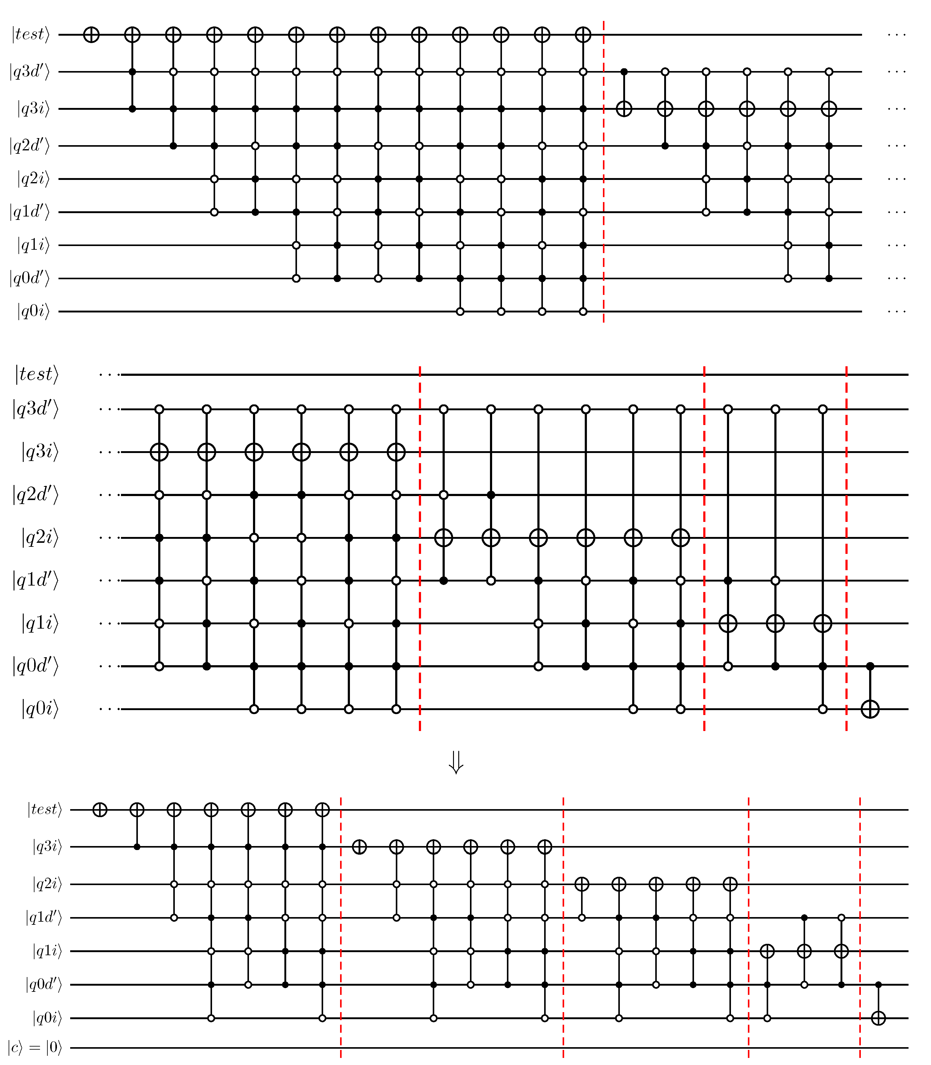
5. Derivation of Parameterised Comparator Circuits

In Section 1, the concept of the comparator step in quantum circuit implementations of a long-division based quantum integer divider was introduced. An example quantum circuit that performs the comparator step for two 4-qubit registers was shown in the top half of Figure 4, where the quantum circuit design followed the work of Xia et al. [33]. In this section, an alternative type of quantum comparator circuits will be derived that facilitates automated quantum circuit reduction steps. Specifically, the aim is to create comparator circuits where, in contrast to the quantum comparator shown in Figure 4, the qubits defining the divisor in the long division will remain unchanged in the circuit and where these qubits can only acts as control qubits in quantum gate operations. For an n-qubit comparator, the derivation works as follows.
  • An ( n + 1 ) -qubit ripple-carry modulo adder of the type introduced by Cuccaro acts as starting point where subtraction of two positive numbers can be achieved by having one of the ( n + 1 ) -qubit inputs represent an n-qubit number in 2’s complement, while the second input will have its leading qubit in state | 0 ;
  • For a specific choice of the n + 1 qubits defining the divisor in 2’s complements representation, qubit specialisation steps of the type previously illustrated in Figure 5 for a 3-qubit modulo adder are applied;
  • The reduced circuits that result from this process represent a subtraction operation by the integer value represented in negative form by the 2’s complement representation;
  • Next, the gate operations in the reduced circuits are sorted in n + 1 groups, where each group represents gate operations affecting the state of each of the n + 1 qubits from the second (remaining) input string;
  • To create the comparator circuit, the group acting on the most-significant qubit of the input qubit register is selected, while the rest of the gate operations can be ignored;
  • The subtractor circuits discussed in Section 6 are similarly created by using the gate operations from each of the n + 1 groups identified.
Since the interest is only in positive divisors defined by a qubit string with the most-significant qubit in state | 1 , 2 n 1 specialised, reduced circuits can be defined. For n = 3 and n = 4 , the top half of Figure 8 and Figure 9, respectively, shows these circuits for specific values of the divisor. As a final step in creating a parameterised comparator, the gate operations from these 2 n 1 specialised circuits are parameterised using the qubits defining the divisor. Two options are available here. First, the use of the n qubits defining the divisor in its original form. Alternatively, the n + 1 qubits defining the divisor in 2’s complement representation can be used. Design choices made in the quantum circuit implementation of the integer divider determine which approach is the most suitable. In this work, for qubit registers where prime superscripts are used in qubit indices, the integer representation is in 2’s complement representation. The next subsections show the quantum comparators for n = 3 , n = 4 , and n = 5 to illustrate the results of the specialisation for divisors represented by an increasing number of qubits.

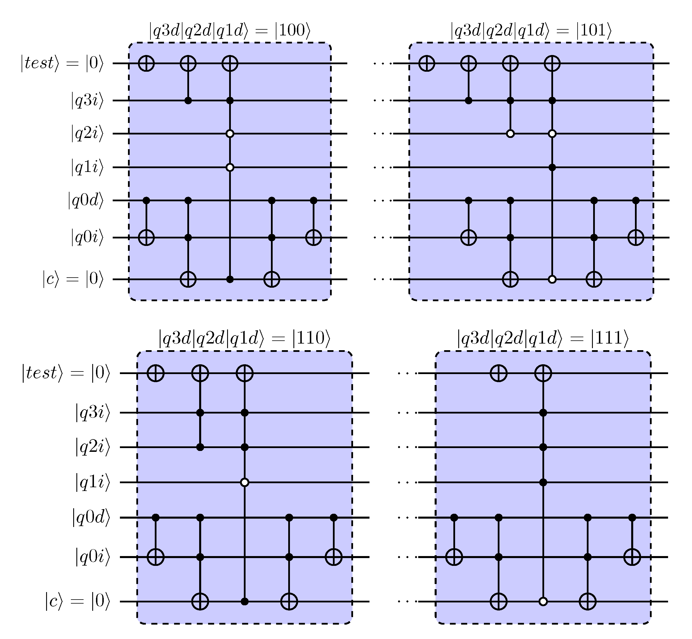
5.1. Comparator Circuits for 3-Qubit Divisor

Based on the reduction in 4-qubit modulo adders, comparator circuits can be derived for quantum dividers with a 3-qubit divisor. Assuming that the divisor is defined by | q 2 d | q 1 d | q 0 d with | q 2 d = | 1 , four different comparator circuits will result. The four comparator circuits are shown at the top of Figure 8.
Using the three divisor qubits as parameters, a parameterised subtractor can be obtained as shown in the bottom half of Figure 8. As will be explained in later sections, the quantum-circuit implementation of quantum integer dividers may employ 2’s complement representation of the divisor qubits. Using the 4-qubit 2’s complement representation | q 3 d | q 2 d | q 1 d | q 0 d , the comparator can be parameterised, as shown in Figure 8. The leading qubit | q 3 d = | 1 as a result of the positive value for divisor assumed here.

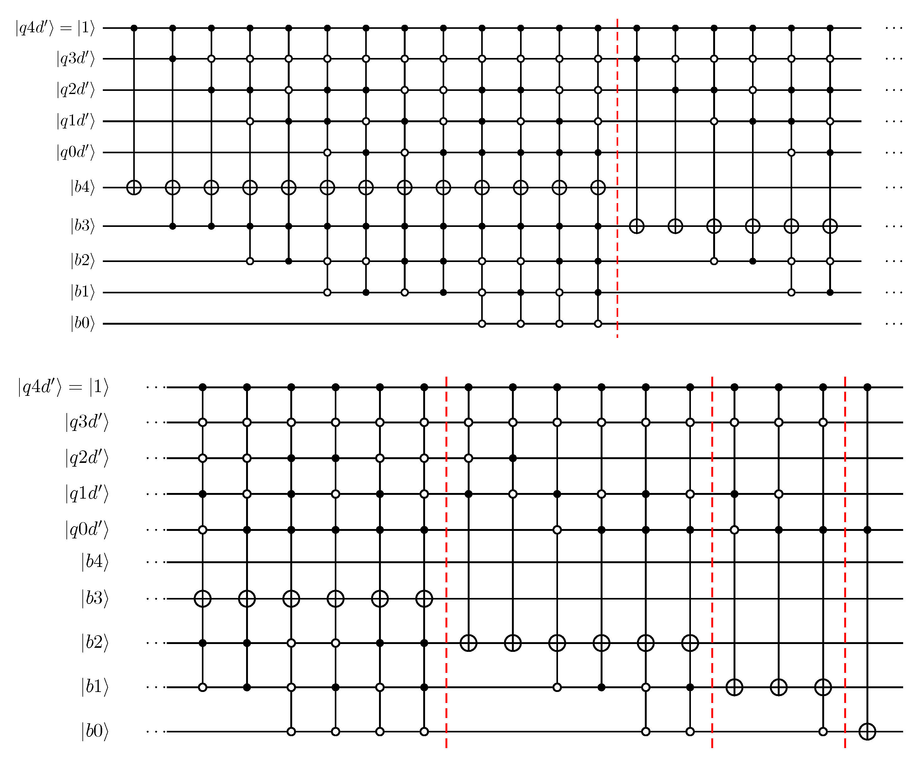
5.2. Comparator Circuits for 4-Qubit Divisor

Based on reduction of 5-qubit modulo adders, comparator circuits can be derived for quantum dividers with 4-qubit divisor using the same approach as in the previous section. Assuming that the divisor is defined by | q 3 d | q 2 d | q 1 d | q 0 d with | q 3 d = | 1 , eight different comparator circuits will result. The top part of Figure 9 summarised the 8 comparator circuits.
The lower part of Figure 9 shows the parameterised comparator circuit for the 4-qubit divisor. The parameterisation is based on the 5-qubit 2’s complement representation of the divisor. As before, the leading qubit | q 4 d in this representation is in state | 1 as a result of the assumption of a positive divisor.

5.3. Comparator Circuits for 5-Qubit Divisor

To further illustrate the parameterised comparator circuits, and to show the increase in circuit complexity for increased number of divisor qubits, the example for 5-qubit divisors is summarized in Figure 10.

6. Derivation of Parameterised Subtractor Circuits

The specialisation of modulo adders used in deriving quantum comparator and subtractor circuits was detailed in Section 5. Here, parameterised subtractors for the example n = 4 (used in division by 4-qubit divisor) are detailed. As explained later in Section 7, the present work considers divider designs where the divisor is represented directly in 2’s complement. For n = 4 , the 5-qubit string representing the divisor in 2’s complement is then considered as the basis for a parameterised 4-qubit subtractor, where, as a result of the assumed positive divisor, | q 4 d = | 1 is guaranteed. The parameterised quantum circuit design is shown in Figure 11. Clearly, the parameterised gate operations acting on the leading qubit of the input register (termed | b 4 here) match the gate operations in the comparator circuit for division by a 4-qubit divisor.
Comparing the quantum circuit in Figure 11 with the quantum circuit implementation of an equivalent ripple-carry adder/subtractor, it is apparent that the complexity of the parameterised quantum circuits is significantly larger in terms of the number of gate operations and, in particular, the number of control qubits used in the majority of gate operations. Therefore, ‘complete’ parameterised circuits as shown in Figure 11 are there to be introduced temporarily during the quantum-circuit transformation with subsequent reduction steps creating smaller, reduced circuits.

7. Applying Circuit Transformations to a Quantum Integer Divider

The quantum circuit implementations for integer dividers considered in this work are based on the concept of long division. Specifically, for a dividend and divisor represented by n qubits, a ( 2 n 1 ) -qubit dividend register (with n 1 least significant qubits in state | 0 ) is created that is then divided by the n-qubit divisor in n long-division steps. This creates an n-qubit representation of the quotient, assuming that the most significant qubit in divisor is in state | 1 . This integer divider can be used in algorithms using fixed-point arithmetic. Additionally, the divider can be used as building block of a floating-point divider where n mantissa bits are used in the floating-point representation. In the quantum circuit implementation, comparator steps are performed that need an additional qubit to act as ‘sign’ qubit. Therefore, for n = 4 , a qubit register with 8 qubits is created to hold the 7-qubit representation of dividend along with this sign qubit. Furthermore, the designs considered are based on the requirement that in the final quantum state, only the qubits representing the result will have been updated, while all other qubits remain in or return to their original state. To achieve this, after the setting the n-qubit result, the steps representing the long division need to be ‘uncomputed’.

7.1. Design 1: Baseline Divider

Figure 3 shows the quantum circuit design of an integer divider based on the long-division approach. The example shown divides a 7-qubit dividend by a 4-qubit divisor. The qubits in this circuit represent the following
| o u t 3 | o u t 2 | o u t 1 | o u t 0 : n   qubits   defining   output | t e s t : qubit   defining   comparator   result | q 4 d : additional   qubit   needed   in   2   complement | q 3 d | q 2 d | q 1 d | q 0 d : n - qubit   representation   of   divisor | q 3 i | q 2 i | q 1 i | q 0 i : n - qubit   representation   of   dividend | c : carry   qubit   in   modulo   adder | q i n 2 | q i n 1 | q i n 0 : n 1   qubits   used   to   create   the   7 - qubit dividend   along   with   | q 3 i | q 2 i | q 1 i | q 0 i
for the quantum circuit implementation illustrated in Figure 3 for the example n = 4 , the circuit complexity in terms of required number of qubits as a function of n is,
n + 2 + 2 n + 1 + ( n 1 ) = 4 n + 2
for n = 4 , a minimum of 18 qubits is, therefore, needed, as shown in Figure 3. For n = 5 , 22 qubits are required. For reference, when employing double-precision arithmetic in the simulators used in the present work, simulating circuits with 28 qubits typically requires 8 GB of memory. Increasing the dividend and divisor representation to n > 6 therefore means that computational resources on a desktop work station are challenged. The quantum circuit implementation of the comparator C and subtractor S u b used in the long-division steps are detailed in Figure 4.
Design 1, presents the following challenges to ‘reducing out’ one or more of the divisor qubits:
  • In the comparator C and its uncomputation U ( C ) , the state of the divisor qubits can temporarily become changed before returning the their original state;
  • The subtractor S u b involves a transformation to 2’s complement formulation for divisor qubits at start and completes with a transformation from 2’s complement to original representation. Along with the further temporary changes to divisor qubit states in the ripple-carry based modulo adder, this greatly complicates static analysis, as outlined previously in Section 4;
  • The ‘downward’ movement of subtractor circuit toward less significant qubits of the dividend in successive long-division steps requires re-arrangement of qubits so that the modular addition on which the subtractor S u b is based can be performed. This further complicates qubit-reduction steps.
The comparator circuit shown in Figure 4 can be reduced by specialisation of one or more (divisor) qubits. Reduction by two qubits is illustrated in Figure 12, while a further reduction by three and four divisor qubits is shown in Figure 13 and Figure 14, respectively. Note that, here, the divisor is represented in its original (4-qubit) form, not in 2’s complement used in later designs. The reductions shown were performed manually, following the same principles outlined previously in Figure 5 for the example of ripple-carry modulo adders. The complexity of step-by-step reduction in these comparator circuits further supports the conclusion drawn in Section 4, that this type of reductions present a major challenge to automation and that, therefore, the alternative approach based on parameterised circuits is preferable.

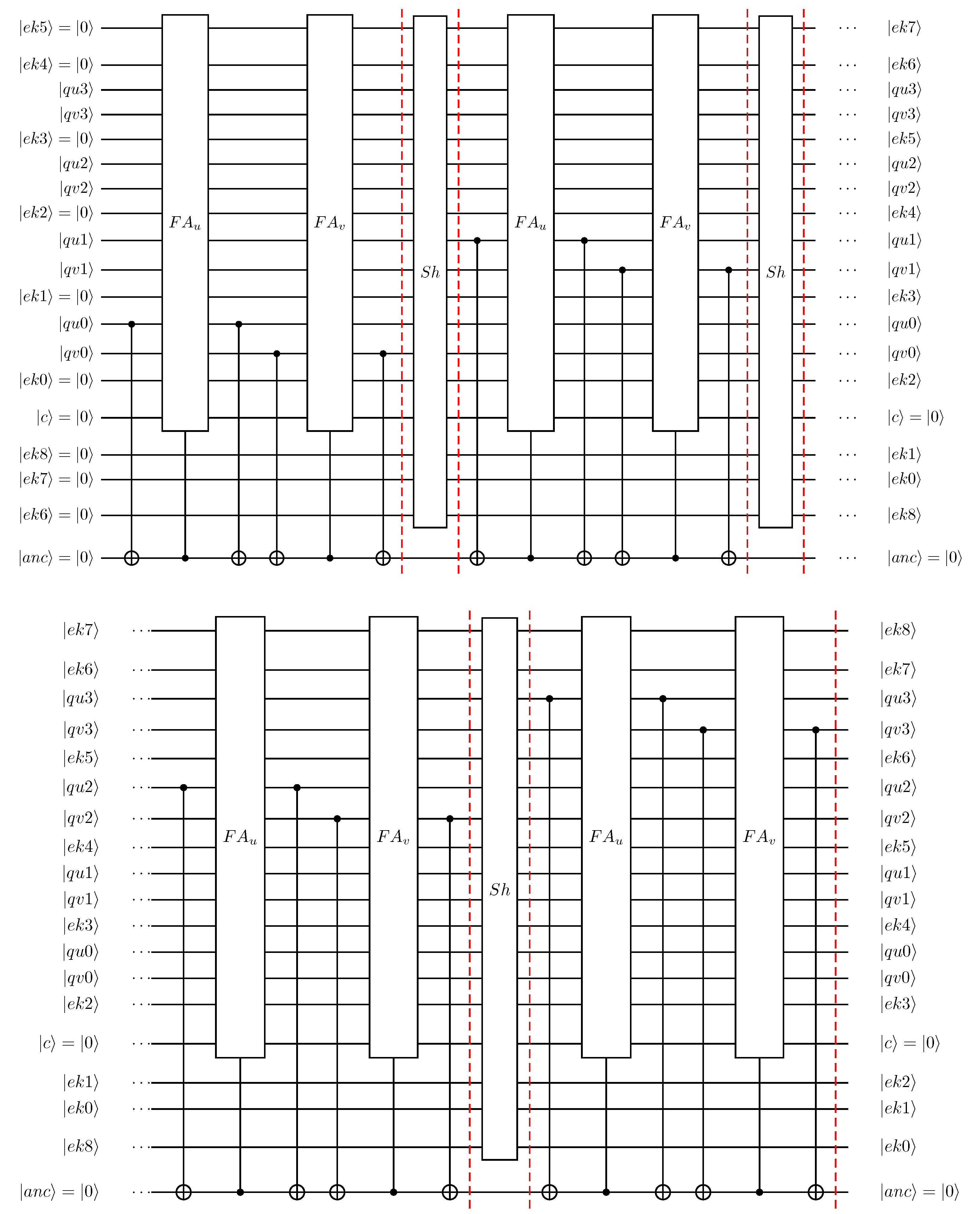
7.2. Design 2: Dividend Register-Shifting Divider

As a first step to facilitating reduction-by-specialisation of divisor qubits, the second design considered here (Design 2) includes a number of important changes relative to Design 1:
  • The ‘downward’ movement of the comparator (and its uncomputations) and subtraction steps for successive long-division steps have been removed by introducing shift operation S h that moves the dividend register one step toward more significant qubits. The quantum circuit implementation of this S h operation, as well as the reverse operation S h ^ (used in the uncomputation steps), was previously discussed in previous work by the authors [30] and follows the work of Jayashree et al. [38];
  • With the changes introduced, the divisor qubits (states) remain in the same position in the qubit register throughout the computation.
The quantum circuit implementation of C (and, therefore, also U ( C ) ), as well as S u b , remains unchanged relative to Design 1. For the quantum circuit implementation illustrated in Figure 15 for the example n = 4 , the circuit complexity in terms of required number of qubits as a function of n is the same for Design 1, i.e., defined by Equation (8).

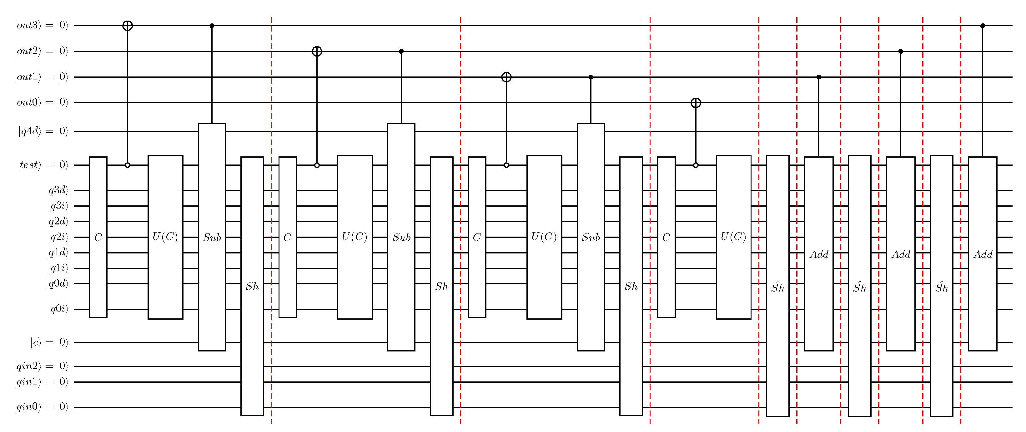
7.3. Design 3: Parameterised Divider

Figure 16 shows a top-level overview of the third design of for a quantum circuit implementation of quantum integer division. For this Design 3, the qubits represent the following:
| o u t 3 | o u t 2 | o u t 1 | o u t 0 : n   qubits   defining   output | t e s t : qubit   defining   comparator   result | q 4 d | q 3 d | q 2 d | q 1 d | q 0 d : ( n + 1 ) - qubit   representation   of   divisor in   2 s   complement   representation | q 3 i | q 2 i | q 1 i | q 0 i : n - qubit   representation   of   dividend | c : carry   qubit   in   modulo   adder | q i n 2 | q i n 1 | q i n 0 : n 1   qubits   used   to   create   the   7 - qubit dividend   along   with   | q 3 i | q 2 i | q 1 i | q 0 i
Therefore, the required number of qubits as a function of n can be written as,
n + 1 + ( n + 1 ) + n + 1 + ( n 1 ) = 4 n + 2
showing that the quantum circuit width remains the same as compared with Design 1 and Design 2.
The definition of the divisor qubits in terms of 2’s complement means that the comparator circuit used in Design 1 and Design 2 cannot be used. Instead, an alternative comparator circuit taking the qubits defining the divisor using 2’s complement is required. One possible way to create such a comparator is shown in Figure 17, where the original circuit following the design of Xia et al. [33] is modified such that the divisor qubits are transformed from 2’s complement representation at input on the left-hand side of the circuit to the regular representation. At the end of the comparator step, the transformation to return to 2’s complement representation for divisor qubits is performed. As can be seen from Figure 17, the additional steps introduced related to 2’s complement conversions add further complexity to the circuit, and therefore making the circuit-width transformation outlined in Figure 12, Figure 13 and Figure 14 for the original form of the comparator even more challenging to automate. This further supports the approach outlined next, where this type of reduction is circumvented.
In Design 3, the key ideas underpinning the automation of qubit reduction-by-specialisation are introduced:
  • For the comparator C and U ( C ) , the original implementation is replaced by an alternative, parameterised quantum circuit implementation where divisor qubits acts as specialisation parameters;
  • For the subtractor S u b , the original implementation is replaced by an alternative, parameterised quantum circuit implementation where divisor qubits acts as specialisation parameters;
  • Design 3 also stores divisor qubits directly in 2’s complement representation. The current analysis shows that using this form of the divisor state makes the parameterisation of the comparator and subtractor more compact than with the original form of divisor.
With these changes, the states of the divisor qubits remain unchanged throughout the computation. This way, automated qubit reduction-by-specialisation becomes a realistic prospect for the tool chain used here. This will be demonstrated in Section 9.
The quantum circuit implementation of the parameterised comparator used in division by 4-qubit divisor is shown in Figure 18, where the states of qubits | q 3 d , | q 2 d , | q 1 d and | q 0 d act as parameters. It should be noted that for the assumed positive divisor, | q 4 d = | 1 in all cases. Based on this parameterisation, a parameterised quantum circuit implementation for the subtractor can be derived as outlined previously in Section 6. For the case of division by a 4-qubit divisor, Figure 19 shows this parameterised quantum circuit implementation.

8. Quantum Circuit Toolchain

One of the general goals of this research is to use reconfigurable hardware to accelerate the simulation of quantum circuits. A quantum circuit toolchain known as the Functional Quantum Toolchain (FQT) [30,46] was developed with the primary purpose of outputting quantum assembly in forms specialised for our custom hardware architectures. Additionally, the toolchain includes utilities for expressing quantum circuits, circuit unit testing, static analysis, and other utilities specific to hardware acceleration. A custom eDSL facilitates expression of quantum circuits. The static analysis tools are particularly relevant to the current work since these form a key part of the automated quantum circuit reduction steps introduced here.

8.1. Circuit Specification and eDSL

FQT is developed in the functional programming language Haskell [47]. In FQT, a circuit (Circ) is defined as a list of gates that comprise the quantum circuit. A core set of gates is supported as primitives. Custom gates can be defined by composition of primitives. Circuits are defined by functions which return a Circ type; list concatenation (the ++ operator in the code snippets below) is used to compose more complex circuits.
At the level of our Haskell eDSL, qubits are given unique identifiers which are used as parameters for our circuit generation functions. Qu represents a single qubit identifier and QReg is an arbitrarily sized list of Qus. High-level operators allow for complex control patterns to be specified for a gate. control(s) takes one control or a list of controls to apply to a gate which follows. negControl(s) are the equivalents for negative controls. For a mix of controls and negative controls, the .== operator is provided to make specification easier. For example ([a,b,c] .== "011") (x d) applies the X gate to qubit d only when a is 0 and b and c are 1. Additional convenience operators include an inverse operator .! which gives the inverse of a quantum circuit by iterating through all gates, finding their inverse, and returning them in reverse. This is particularly useful when using the uncomputation pattern.
As a brief example of circuit specification in the eDSL, Figure 20 defines a specialised 4-qubit comparator circuit used to check if the input value is less than 9. Line 1 describes the type signature of the lt9q4 circuit generator, ascertaining it takes a quantum register QReg and a single qubit Qu, and returns a Circ. As QReg is an arbitrarily sized quantum register, the Line 2 pattern matches on its contents and tells the compiler to expect exactly four elements. Lines 3, 4, and 5 define and concatenate the three sub-circuits which form the comparator. Each of x, cnot, and .== are (informally) defined as ‘circuit generators’. In general, a circuit generator takes any number of arguments and returns a Circ. High-level operators (including .== are defined as functions which take at least one Circ argument.
The internal representation (IR) of a circuit defined in this way is simply a list of gates defined over some set of primitive gate types. Figure 21 shows the IR of the example 4-bit comparator, specialised for less-than-9.

8.2. Static Analysis to Reduce Qubit Count

A key component of our toolchain is the static analyser, which enables reducing a circuit’s depth by specialising the circuit for specific inputs for some qubits. In the presented version, the qubits to be reduced cannot have gates applied to them which change their state; they can only be used as controls or negative controls. To perform the reduction, the analyser iterates through the circuit gate-by-gate, checking if each gate’s controls satisfy the input specialisation; in the case they do, their controls are modified to no longer include the specialisation qubits and they are are added to the reduced circuit. If the controls are not satisfied, the gate is not included in the final circuit.

8.3. Testing and Verification

Verification of circuits is performed by implementing unit tests that comprise the following steps. First, for the specific case considered, the quantum register is initialized in the simulator, followed by the simulation of the quantum circuit. Then, the obtained output is checked against the intended output for the specified input. The example circuits considered here employ computational basis encoding, while the gate operations are restricted to logic gates, i.e., N O T with any number of control qubits. For this type of circuits, the simulations in the verification can be performed using the logic-based simulator described earlier. For more general circuits, as well as quantum circuits defining algorithms employing amplitude-based encoding, the verification is performed using a full-state-vector simulator. A QCTestSuite is defined as a set of tests with different preparations and expectations for the same circuit. It takes a string descriptor, the circuit to test, the full register over which to apply the circuit, and a list of QCTests. A QCTest is simply a string descriptor, a list of initial qubit register states, and a list of expected output qubit register states. An example of manually specifying tests suites is given in Figure 22. In this example, Line 1 defines leftShiftTestSuite as a static QCTestSuite. Line 3 declares the register over which the circuit tests are to be ran. Line 4 declares the test suite itself, passing it the circuit (leftShift reg), and the register. Two test cases follow: lines 6 and 9 specify the preparations of the test cases, each preparing reg in a different state; lines 7 and 10 specify the intended output state of qubit register of the tests.
Manually specifying test cases can be tedious, and for larger circuits is very impractical. However, since the testing framework is implemented and used in Haskell, native Haskell features, such as list comprehensions, enable automated test generation, as shown in Figure 23.

9. Demonstration of Reduction of Integer Divider

This section illustrates the implementation of the full long division circuit (Figure 16) in the FQT toolchain and demonstrates the derivation and verification of its reduced forms.

9.1. Parameterised Integer Divider Implementation in Toolchain—Before Circuit Transformation

Figure 24 illustrates the implementation of the integer divider quantum circuit presented in Figure 16 in the FQT eDSL. As demonstrated in the figure, the division of a 7-bit dividend by a 4-bit divisor can be composed from three compare, subtract, and shift blocks and one compare block. To return qubits acting as workspace to the original | 0 state, a 3-step uncomputation of controlled subtractions (with associated reversed shifts) is performed.
The compare block uses a comparator circuit to set the | t e s t = | 1 qubit if the integer value of the considered 4-bit sub-string of the dividend is less than the divisor integer value. A controlled-X gate copies the result of the comparison to the output qubit for the considered long-division step. The uncomputation of the comparison is then performed to restore the test qubit to its original state.
The compare, subtract, and shift block (compareSubtractShiftBlock) uses this compare block and applies the subtraction circuit controlled by the out qubit (which now carries the result of the comparison). Finally, the left shift operator is applied to the dividend register (including | t e s t and | q i n ) to prepare the state for the next long division step. Three of these compare, subtract, and shift blocks are used (lines 9–11), each using an out qubit with the next lower significance in the | o u t register as the output of the comparator. The last compare block (without a subtractor) on line 12 sets the least significant out qubit. Finally, the uncomputation of the subtractions and shifts is performed on lines 13–15 by declaring three shiftUnsubtractBlocks. These blocks are defined as a right shift over the previously shifted qubits, followed by the inverse circuit of the subtractor. These operations are chained together to match the blocks in Figure 16.

9.2. Specialised Integer Divider

To specialise the circuit for particular values of the divisor, the specialisation function (specialiseQCircForQubitValues) is used, applying the static analysis methods discussed in Section 8.2 to reduce the divisor qubits. First the full circuit is created, and then passed to the specialiser, as shown in Figure 25. This high-order function expects three arguments, including the qubits over which to specialise, expressed as a QReg; a bit string indicating their initial values; and the circuit to specialise. The sizes of the register and the bit string must match and the circuit must not contain gates which change the state of the specialisation qubits, otherwise an error will be thrown. In the example shown, the function generating the specialised circuit now takes an integer representing the value of b (the divisor) instead of a register bReg. On line 7, an intermediate register bReg is created to pass to the generator of the full function on line 8. On line 9, the bit register is prepared by calling the utility function paddedTwoComplementBitString to obtain the 2’s complement representation of b (as required by the long division algorithm). Finally, the specialisation function is called to generate the qubit-reduced circuit.
Figure 26 and Figure 27 show the first blocks of a parameterised divider that has been fully specialised on the divider qubits. These are the initial comparison and subtraction blocks which set the most significant out qubit. Figure 26 shows the block specialised for a divisor value of 9, while Figure 27 shows the specialised circuit for a divisor value of 11 as illustrative examples.

9.3. Results

The primary goal of this work is to introduce techniques for facilitating the reduction in quantum circuit width (required qubit count) through static analysis. In this section, results from testing the full and specialised circuits are presented.
The toolchain’s testing components are used to verify the correctness of the generated dividers using the logic-based circuit simulator. Both the full divider and the specialised versions were tested.
We start by verifying the functionality of the non-specialised divider demonstrated in Figure 16 (Design 3). The circuit is constructed as described in the previous section by the code in Figure 24. Table 1 shows a sample from the results of running an automatically generated test suite for this circuit. The first column shows the integer division performed, while the second and third columns show the qubit register state after initialization and completion of the circuit simulation, respectively. For clarity, the final column summarizes the 4-qubit output from the long-division performed. For all cases considered, the obtained output from the quantum circuit simulator used in verification matched the intended output.
We also verify the functionality of a divider with a fully specialised divisor. It is important to note that, unlike the full divider test suite which operates only on one circuit, the specialised dividers require specific quantum circuits for each value of the divisor. Thus, several test suites are constructed (this is automated with list comprehensions, as described in Figure 23), one for each divisor. Table 2 shows the results of testing these circuits, collated from multiple test suites.

9.4. Discussion of Results—Implication for Wider Range of Circuits

As discussed in Section 1, the present work on circuit reduction steps for quantum arithmetic operations is motivated by the fact that such arithmetic operations are often an important part of a wide range of larger and more general quantum algorithms. The development and evaluation of these larger quantum algorithms typically involves large-scale full-state vector circuit simulations, e.g., to check correctness, sensitivity of quantum gate errors and effect of quantum decoherence errors. High-performance computing resources commonly available to quantum algorithm developers typically limit the qubit count to 30–35, so that reductions of multiple qubits that are only involved in quantum arithmetic operations create much needed reduced memory requirements.
Considering the small example problems discussed here, for the integer divider the quantum circuit width was reduced from 17 qubits in the original circuit (going down to 16 when parameterised, since a carry qubit used in the Cuccaro adders could be removed) to 12 in the ‘fully’ reduced circuit (i.e., specialised for a specific value of divisor). For a circuit simulator using full state vector, this results in a useful reduction in memory by a factor of 32.
The FQT toolchain was also used to inspect the gate complexity of the circuits that result from the various eDSL definitions above. To summarise the results of proposed transformation, the previously considered integer division circuit for a 7-qubit dividend and 4-qubit divisor is detailed in Table 3. The baseline circuit uses Cuccaro modulo adders. For a 4-qubit divisor, the reduction step can then reduce the qubit count by 5 since the carry qubit from the Cuccaro adder can also be removed. The gate count reduction relative to the baseline is dependent on the particular choice of the divisor value, as shown in the table for two example values. The baseline long division circuit without parameterisation requires 674 gates to implement. The implemented parameterised long division circuit produced by the listing in Figure 24 requires 1612 gate operations, while the fully reduced divider generated by Figure 25 requires only 252 gates for the dividing by 9 example and 296 gates for dividing by 11.
Today, it is feasible to simulate 20–25 qubits on a typical everyday laptop. For larger problems up to approximately 35 qubits, researchers using full-state vector simulators require distributed computing facilities often available in research centres and universities. For even larger circuit width, regional or national high-performance computing facilities are required, so that circuits simulations cannot be performed routinely in an algorithm development process where many repeated simulations are needed.
It is important to recognise that while the implemented examples here are four dividers with 4 divisor bits, the techniques described are applicable to dividers of any size. For example, the complexity analysis in Section 7.1 can be used to determine that a divider with an 8 bit divider would require a 34 qubit circuit to run (requiring over 137 GB of memory to simulate with 32-bit floating point precision). Using the described techniques, 8 qubits can be reduced, requiring only 26 qubits or 0.53 GB to be simulated. The quantum integer divider was used here for illustration purposes; the proposed reduction involving parameterisation and static analysis applies far more widely to quantum arithmetic operations.
The quantum circuits for integer arithmetic can naturally be extended to arithmetic of real numbers using fixed-point representation. Additionally, in ongoing work by one of the authors [29,31], arithmetic operations based on computational basis encoding is used for floating-point operations. In the interest of brevity, this was not discussed in the present work. However, the introduced quantum circuit transformations can be applied to this type of quantum circuit for floating-point arithmetic as well. This will be considered in future work.
The introduced circuit width reductions can therefore be of great benefit to algorithm developers by facilitating simulations of larger circuits on available computing resources.

10. Conclusions and Future Work

Quantum circuit transformation and parameterisation techniques were introduced that specifically target facilitating static analysis of quantum circuits for the purpose of circuit width reduction (reduced qubit count). Using these techniques, quantum circuits which would otherwise require excessive amounts of memory can be analysed on full state vector simulators. The introduced transformation approach can be applied to a wide range of quantum algorithms where quantum arithmetic operations form part of the computational work performed by the algorithm. The transformations are demonstrated for an exemplar quantum integer divider and its constituent parts, the comparators and subtractors. The first step in transformation involves a user-directed replacement of an quantum-circuit block performing arithmetic by a parameterised circuit performing this operation. In the next step, the presented static analysis tool can then automatically eliminate any qubits which are used only as controls for user-specified given inputs. As demonstrated for the integer divider example, using this approach, reductions in quantum circuit width can be achieved that match reductions obtained by manual reduction-by-specialisation.
While the introduced transformation approach is specific to quantum circuit operations performing arithmetic in the computational basis, it is clear that the specialised circuits can be used as building blocks in larger circuits which go beyond the computational basis. Furthermore, it is important to note that the transformation approach is not limited to the particular tool chain employed here, i.e., it is expected that other tool chains designed to perform transformations on circuits specified in other DSLs can be extended to include the transformation approach discussed here.
In future work, the introduced techniques will be extended to a wider range of quantum algorithms with embedded quantum arithmetic operations. Additionally, quantum algorithms for scientific computations using floating-point arithmetic will be targeted.

Author Contributions

Circuit Transformation and Reduction Concepts, R.S.; derivation of Parameterised Comparator, Subtractor, and Divider circuits, R.S.; Project administration and supervision, R.S. and W.V.; Functional Quantum Toolchain, Y.M.; Implementation and validation of circuits, Y.M.; Writing—review and editing, W.V. All authors have read and agreed to the published version of the manuscript.

Funding

This research received no external funding.

Institutional Review Board Statement

Not applicable.

Informed Consent Statement

Not applicable.

Data Availability Statement

The data being made available for this work is in the form of the FQT code which generates and processes the discussed circuits. The code is available on Zenodo: https://zenodo.org/record/7645972#.Y-3-6S-l1B0 (accessed on 3 February 2023).

Acknowledgments

The authors acknowledge financial support received from the University of Glasgow in the form of a Ph.D. scholarship for Y.M.

Conflicts of Interest

The authors declare no conflict of interest.

Abbreviations

The following abbreviations are used in this manuscript:
QCQuantum Computing
FQTFunctional Quantum Toolchain
DSLDomain Specific Language
eDSLEmbedded Domain Specific Language

References

  1. Nielsen, M.; Chuang, I. Quantum Computation and Quantum Information: 10th Anniversary Edition; Cambridge University Press: Cambridge, UK, 2010. [Google Scholar]
  2. Preskill, J. Quantum Computing in the NISQ era and beyond. Quantum 2018, 2, 79. [Google Scholar] [CrossRef]
  3. IBM unveils 127-qubit computer. Phys. World 2021, 34, 13ii. [CrossRef]
  4. Gambetta, J. IBM Quantum Roadmap to Build Quantum-Centric Supercomputers. 2022. Available online: https://research.ibm.com/blog/ibm-quantum-roadmap-2025 (accessed on 28 April 2023).
  5. Guerreschi, G.G.; Hogaboam, J.; Baruffa, F.; Sawaya, N.P.D. Intel Quantum Simulator: A cloud-ready high-performance simulator of quantum circuits. Quantum Sci. Technol. 2020, 5, 34007. [Google Scholar] [CrossRef]
  6. Childs, A.M.; Schoute, E.; Unsal, C.M. Circuit Transformations for Quantum Architectures. In Proceedings of the TQC 2019, College Park, MD, USA, 3–7 June 2019; Volume 135, pp. 1–24. [Google Scholar] [CrossRef]
  7. Boixo, S.; Isakov, S.V.; Smelyanskiy, V.N.; Neven, H. Simulation of low-depth quantum circuits as complex undirected graphical models. arXiv 2017, arXiv:1712.05384. [Google Scholar] [CrossRef]
  8. Chen, J.; Zhang, F.; Huang, C.; Newman, M.; Shi, Y. Classical Simulation of Intermediate-Size Quantum Circuits. arXiv 2018, arXiv:1805.01450. [Google Scholar] [CrossRef]
  9. Schutski, R.; Lykov, D.; Oseledets, I. Adaptive algorithm for quantum circuit simulation. Phys. Rev. A 2020, 101, 42335. [Google Scholar] [CrossRef]
  10. Pednault, E.; Gunnels, J.A.; Nannicini, G.; Horesh, L.; Magerlein, T.; Solomonik, E.; Draeger, E.W.; Holland, E.T.; Wisnieff, R. Pareto-Efficient Quantum Circuit Simulation Using Tensor Contraction Deferral. arXiv 2017, arXiv:1710.05867. [Google Scholar] [CrossRef]
  11. Chen, Z.Y.; Zhou, Q.; Xue, C.; Yang, X.; Guo, G.C.; Guo, G.P. 64-qubit quantum circuit simulation. Sci. Bull. 2018, 63, 964–971. [Google Scholar] [CrossRef]
  12. Li, R.; Wu, B.; Ying, M.; Sun, X.; Yang, G. Quantum Supremacy Circuit Simulation on Sunway TaihuLight. IEEE Trans. Parallel Distrib. Syst. 2018, 31, 805–816. [Google Scholar] [CrossRef]
  13. Qiskit Contributors. Qiskit: An Open-source Framework for Quantum Computing; Zenodo: Geneva, Switzerland, 2023. [Google Scholar] [CrossRef]
  14. Green, A.S.; LeFanu, P.; Ross, N.J.; Selinger, P.; Valiron, B. Quipper: A Scalable Quantum Programming Language. ACM SIGPLAN Not. 2013, 48, 333–342. [Google Scholar]
  15. Cross, A.W.; Bishop, L.S.; Smolin, J.A.; Gambetta, J.M. Open Quantum Assembly Language. arXiv 2017, arXiv:1707.03429. [Google Scholar]
  16. Cross, A.W.; Javadi-Abhari, A.; Alexander, T.; de Beaudrap, N.; Bishop, L.S.; Heidel, S.; Ryan, C.A.; Smolin, J.; Gambetta, J.M.; Johnson, B.R. OpenQASM 3: A broader and deeper quantum assembly language. ACM Trans. Quantum Comput. 2021, 3, 12. [Google Scholar] [CrossRef]
  17. Killoran, N.; Izaac, J.; Quesada, N.; Bergholm, V.; Amy, M.; Weedbrook, C. Strawberry Fields: A Software Platform for Photonic Quantum Computing. Quantum 2019, 3, 129. [Google Scholar] [CrossRef]
  18. Bergholm, V.; Izaac, J.; Schuld, M.; Gogolin, C.; Ahmed, S.; Ajith, V.; Alam, M.S.; Alonso-Linaje, G.; AkashNarayanan, B.; Asadi, A.; et al. PennyLane: Automatic differentiation of hybrid quantum-classical computations. arXiv 2018, arXiv:quant-ph/1811.04968. [Google Scholar]
  19. Hooyberghs, J. Q# Language Overview and the Quantum Simulator. In Introducing Microsoft Quantum Computing for Developers; Apress: Berkeley, CA, USA, 2022; pp. 121–167. [Google Scholar] [CrossRef]
  20. Shor, P. Algorithms for quantum computation: Discrete logarithms and factoring. In Proceedings of the 35th Annual Symposium on Foundations of Computer Science, Santa Fe, NM, USA, 20–22 November 1994; pp. 124–134. [Google Scholar] [CrossRef]
  21. Partsch, H.; Steinbrüggen, R. Program transformation systems. ACM Comput. Surv. 1983, 15, 199–236. [Google Scholar] [CrossRef]
  22. Lattner, C.; Amini, M.; Bondhugula, U.; Cohen, A.; Davis, A.; Pienaar, J.; Riddle, R.; Shpeisman, T.; Vasilache, N.; Zinenko, O. MLIR: Scaling compiler infrastructure for domain specific computation. In Proceedings of the 2021 IEEE/ACM International Symposium on Code Generation and Optimization (CGO), Seoul, Republic of Korea, 27 February–3 March 2021; IEEE: Piscataway, NJ, USA, 2021; pp. 2–14. [Google Scholar]
  23. Bastoul, C.; Cohen, A.; Girbal, S.; Sharma, S.; Temam, O. Putting polyhedral loop transformations to work. In Proceedings of the Languages and Compilers for Parallel Computing: 16th International Workshop (LCPC 2003), College Station, TX, USA, 2–4 October 2003; Springer: Berlin/Heidelberg, Germany, 2004; pp. 209–225. [Google Scholar]
  24. Vanderbauwhede, W. Making legacy Fortran code type safe through automated program transformation. J. Supercomput. 2022, 78, 2988–3028. [Google Scholar] [CrossRef]
  25. Todorova, B.; Steijl, R. Quantum Algorithm for the collisionless Boltzmann equation. J. Comp. Phys. 2020, 409, 109347. [Google Scholar] [CrossRef]
  26. Steijl, R. Quantum Algorithms for Fluid Simulations. In Advances in Quantum Communication and Information Bulnes; Bulnes, F., Ed.; IntechOpen: London, UK, 2020; ISBN 978-1-78-985268-4. [Google Scholar] [CrossRef]
  27. Budinski, L. Quantum algorithm for the advection–diffusion equation simulated with the lattice Boltzmann method. Quantum Inf. Process. 2021, 20, 57. [Google Scholar] [CrossRef]
  28. Itani, W.; Succi, S. Analysis of Carleman Linearization of Lattice Boltzmann. Fluids 2022, 7, 24. [Google Scholar] [CrossRef]
  29. Steijl, R. Quantum algorithms for nonlinear equations in fluid mechanics. In Quantum Computing and Communications; Zhao, Y., Ed.; IntechOpen: London, UK, 2022; ISBN 978-1-83-968133-2. [Google Scholar] [CrossRef]
  30. Moawad, Y.; Vanderbauwhede, W.; Steijl, R. Investigating hardware acceleration for simulation of CFD quantum circuits. Front. Mech. Eng. 2022, 8. [Google Scholar] [CrossRef]
  31. Steijl, R. Quantum Circuit Implementation of Multi-Dimensional Non-Linear Lattice Models. Appl. Sci. 2023, 13, 529. [Google Scholar] [CrossRef]
  32. Overton, M. Numerical Computing with IEEE Floating Point Arithmetic, 1st ed.; SIAM: Philadelphia, PA, USA, 2001. [Google Scholar]
  33. Xia, H.; Li, H.; Zhang, H.; Liang, Y.; Xin, J. Novel multi-bit quantum comparators and their application in image binarization. Quantum Inf. Process. 2019, 18, 229. [Google Scholar] [CrossRef]
  34. Shan-zhi, L. Design of Quantum Comparator Based on Extended General Toffoli Gates with Multiple Targets. Comput. Sci. 2012, 39, 302–306. [Google Scholar]
  35. Vudadha, C.; Phaneendra, P.S.; Sreehari, V.; Ahmed, S.E.; Muthukrishnan, N.M.; Srinivas, M. Design of Prefix-Based Optimal Reversible Comparator. In Proceedings of the 2012 IEEE Computer Society Annual Symposium on VLSI, Amherst, MA, USA, 19–21 August 2012; pp. 201–206. [Google Scholar] [CrossRef]
  36. Orts, F.; Ortega, G.; Cucura, A.C.; Filatovas, E.; Garzón, E.M. Optimal fault-tolerant quantum comparators for image binarization. J. Supercomput. 2021, 77, 8433–8444. [Google Scholar] [CrossRef]
  37. Yuan, S.; Gao, S.; Wen, C.; Wang, Y.; Qu, H.; Wang, Y. A novel fault-tolerant quantum divider and its simulation. Quantum Inf. Process. 2022, 21, 182. [Google Scholar] [CrossRef]
  38. Jayashree, H.; Thapliyal, H.; Arabnia, H.; Agrawal, V. Ancilla-input and garbage-output optimized design of a reversible quantum integer multiplier. J. Supercomput. 2016, 72, 1477–1493. [Google Scholar] [CrossRef]
  39. Dutta, S.; Bhattacharjee, D.; Chattopadhyay, A. Quantum circuits for Toom-Cook multiplication. Phys. Rev. A 2018, 98, 012311. [Google Scholar] [CrossRef]
  40. Munoz-Coreas, E.; Thapliyal, H. Quantum Circuit Design of a T-count Optimized Integer Multiplier. IEEE Trans. Comput. 2019, 68, 729–739. [Google Scholar] [CrossRef]
  41. Orts, F.; Ortega, G.; Filatovas, E.; Garzón, E.M. Implementation of three efficient 4-digit fault-tolerant quantum carry lookahead adders. J. Supercomput. 2022, 78, 13323–13341. [Google Scholar] [CrossRef]
  42. Gayathri, S.; Kumar, R.; Dhanalakshmi, S.; Dooly, G.; Duraibabu, D.B. T-Count Optimized Quantum Circuit Designs for Single-Precision Floating-Point Division. Electronics 2021, 10, 703. [Google Scholar] [CrossRef]
  43. Draper, T.G. Addition on a Quantum Computer. arXiv 2000, arXiv:quant-ph/0008033. [Google Scholar] [CrossRef]
  44. Ruiz-Perez, L.; Garcia-Escartin, J. Quantum arithmetic with the quantum Fourier transform. Quantum Inf. Process. 2017, 16, 152. [Google Scholar] [CrossRef]
  45. Cuccaro, S.A.; Draper, T.G.; Kutin, S.A.; Moulton, D.P. A new quantum ripple-carry addition circuit. arXiv 2004, arXiv:quant-ph/0410184. [Google Scholar] [CrossRef]
  46. Moawad, Y.; Vanderbauwhede, W.; Steijl, R. Transformations for accelerator-based quantum circuit simulation in Haskell. arXiv 2022, arXiv:2210.12703. [Google Scholar] [CrossRef]
  47. Marlow, S. Haskell 2010 Language Report. 2010. Available online: http://www.haskell.org/ (accessed on 28 April 2023).
Figure 1. Illustration of simple two-qubit quantum circuits.
Algorithms 16 00241 g001
Figure 2. Quantum circuit design for evaluation of u 2 + v 2 based on 4-qubit fixed-point representation of velocities u (defined by | q u 3 | q u 2 | q u 1 | q u 0 ) and v (defined by | q v 3 | q v 2 | q v 1 | q v 0 ). Upon completion on right-hand side of circuit, the kinetic energy is represented by 9 qubits | e k 8 | e k 7 | | e k 0 . F A u and F A v are modified 4-qubit full adders and S h performs incremental shifts on output register.
Algorithms 16 00241 g002
Figure 3. Quantum integer divider: top-level overview of quantum circuit implementation of quantum integer division. Example shown for 4-qubit representation of dividend, divisor, and output.
Algorithms 16 00241 g003
Figure 4. Quantum integer divider: quantum circuit implementation of comparator C and subtractor S u b . Example shown for 4-qubit representation of dividend, divisor, and output. Sub-circuits on left- and right-hand side perform transforms to/from 2’s complement for divisor qubits.
Algorithms 16 00241 g004
Figure 5. Specialised modulo 3-qubit modulo adders. Example shown for | a 2 | a 1 | a 0 = | 101 . Can be used to subtract 3 from integer defined by binary representation of | b 2 | b 1 | b 0 .
Algorithms 16 00241 g005
Figure 6. Illustration of reduction operation on divisor qubits in subtractor circuit. Example shows specialisation of three most-significant qubits | q 4 d | q 3 d | q 2 d to | 101 . In reduced quantum circuit shown at bottom, the M A J and U M A sub-circuits have been expanded for clarity.
Algorithms 16 00241 g006
Figure 7. Illustration of automated reduction of a quantum modulo adder in parameterised form. Example shows specialisation of three most-significant qubits | q 4 d | q 3 d | q 2 d to | 101 .
Algorithms 16 00241 g007
Figure 8. Comparator circuits for use in quantum dividers with 3-qubit divisor. Parameterisation with divisor qubits and with 2’s complement representation of divisor shown in lower half.
Algorithms 16 00241 g008
Figure 9. Comparator circuits for use in quantum dividers with 4-qubit divisor. Parameterisation with 2’s complement of the divisor is shown in the lower half.
Algorithms 16 00241 g009
Figure 10. Parameterised comparator circuit for division by 5-qubit divisor. Parameterisation employs qubits in 2’s complement representation.
Algorithms 16 00241 g010
Figure 11. Subtractor circuit for 4-qubit quantum divider. Gate operations are parameterised with divisor qubit state represented in 2’s complement.
Algorithms 16 00241 g011
Figure 12. Reduction-by-specialisation of comparator circuit introduced by Xia et al. [33]. Reduction by two qubits.
Algorithms 16 00241 g012
Figure 13. Reduction-by-specialisation of comparator circuit introduced by Xia et al. [33]. Reduction by three qubits.
Algorithms 16 00241 g013
Figure 14. Reduction-by-specialisation of comparator circuit introduced by Xia et al. [33]. Reduction by four qubits.
Algorithms 16 00241 g014
Figure 15. Quantum integer divider design 2: top-level overview of quantum circuit implementation of quantum integer division. Example shown for 4-qubit representation of dividend, divisor, and output. The quantum circuit implementation of C and S u b same as in Design 1.
Algorithms 16 00241 g015
Figure 16. Quantum integer divider Design 3: top-level overview of quantum circuit implementation of quantum integer division. Example shown for 4-qubit representation of dividend, divisor, and output. Based on parameterised quantum circuit implementation of C, U ( C ) , and S u b .
Algorithms 16 00241 g016
Figure 17. 4-qubit comparator based on design of Xia et al. [33] reworked to have divisor quantum state in terms of 2’s complement.
Algorithms 16 00241 g017
Figure 18. Quantum circuit implementation of comparator C as used in Design 3 for 4-qubit representation of dividend, divisor and output.
Algorithms 16 00241 g018
Figure 19. Quantum circuit implementation of subtractor S u b as used in Design 3 for 4-qubit representation of dividend, divisor and output.
Algorithms 16 00241 g019
Figure 20. A specialised four-qubit less than 9 operator expressed in the FQT eDSL. On the right is the circuit diagram of the comparator for reference.
Algorithms 16 00241 g020
Figure 21. Specialised 4-bit comparator (9) in the Toolchain IR. The X gates on r 2 , r 1 , and r 0 are there to enable the negative controls on these qubits.
Algorithms 16 00241 g021
Figure 22. Manually specifying test cases for a 4-qubit left shift operator.
Algorithms 16 00241 g022
Figure 23. Automating the generation of test cases for a parameterised subtractor circuit. As binary operations such as subtraction and comparison take two inputs, to fully iterate over the possible test cases, two list comprehensions are used. To keep the code clear and maintainable, two functions are used, each using a list comprehension to iterate on one of the inputs.
Algorithms 16 00241 g023
Figure 24. Long division operator specification.
Algorithms 16 00241 g024
Figure 25. Specialisation of the long division circuit.
Algorithms 16 00241 g025
Figure 26. Fully specialised quantum circuit implementation of integer division. Reduction for | q 4 d | q 3 d | q 2 d | q 1 d | q 0 d = | 10111 represents cases where the divisor is 9. First step of long division.
Algorithms 16 00241 g026
Figure 27. Fully specialised quantum circuit implementation of integer division. Reduction for | q 4 d | q 3 d | q 2 d | q 1 d | q 0 d = | 10101 represents cases where the divisor is 11. First step of long division.
Algorithms 16 00241 g027
Table 1. Full Design 3 long division divider testing results sample.
| out 3 | out 2 | out 1 | out 0 | test | b 3 | a 3 | b 2 | a 2 | b 1 | a 1 | b 0 | a 0 | qin 2 | qin 1 | qin 0
OperationInputOutputUnpacked | out
64 / 9 | 0 | 0 | 0 | 0 | 0 | 0 | 1 | 1 | 0 | 1 | 0 | 1 | 0 | 0 | 0 | 0 | 0 | 1 | 1 | 1 | 0 | 0 | 1 | 1 | 0 | 1 | 0 | 1 | 0 | 0 | 0 | 0 | 0111 (7)
72 / 10 | 0 | 0 | 0 | 0 | 0 | 0 | 1 | 1 | 0 | 1 | 0 | 0 | 1 | 0 | 0 | 0 | 0 | 1 | 1 | 1 | 0 | 0 | 1 | 1 | 0 | 1 | 0 | 0 | 1 | 0 | 0 | 0 | 0111 (7)
96 / 11 | 0 | 0 | 0 | 0 | 0 | 0 | 1 | 1 | 1 | 0 | 0 | 1 | 0 | 0 | 0 | 0 | 1 | 0 | 0 | 0 | 0 | 0 | 1 | 1 | 1 | 0 | 0 | 1 | 0 | 0 | 0 | 0 | 1000 (8)
104 / 12 | 0 | 0 | 0 | 0 | 0 | 0 | 1 | 1 | 1 | 0 | 0 | 0 | 1 | 0 | 0 | 0 | 1 | 0 | 0 | 0 | 0 | 0 | 1 | 1 | 1 | 0 | 0 | 0 | 1 | 0 | 0 | 0 | 1000 (8)
112 / 13 | 0 | 0 | 0 | 0 | 0 | 0 | 1 | 0 | 1 | 1 | 1 | 1 | 0 | 0 | 0 | 0 | 1 | 0 | 0 | 0 | 0 | 0 | 1 | 0 | 1 | 1 | 1 | 1 | 0 | 0 | 0 | 0 | 1000 (8)
80 / 14 | 0 | 0 | 0 | 0 | 0 | 0 | 1 | 0 | 0 | 1 | 1 | 0 | 0 | 0 | 0 | 0 | 0 | 1 | 0 | 1 | 0 | 0 | 1 | 0 | 0 | 1 | 1 | 0 | 0 | 0 | 0 | 0 | 0101 (5)
104 / 15 | 0 | 0 | 0 | 0 | 0 | 0 | 1 | 0 | 1 | 0 | 0 | 1 | 1 | 0 | 0 | 0 | 0 | 1 | 1 | 0 | 0 | 0 | 1 | 0 | 1 | 0 | 0 | 1 | 1 | 0 | 0 | 0 | 0110 (6)
Table 2. Specialised-divisor long division testing results sample.
| out 3 | out 2 | out 1 | out 0 | test | a 3 | a 2 | a 1 | a 0 | qin 2 | qin 1 | qin 0
OperationInputOutputUnpacked | out
64 / 9 | 0 | 0 | 0 | 0 | 0 | 1 | 0 | 0 | 0 | 0 | 0 | 0 | 0 | 1 | 1 | 1 | 0 | 1 | 0 | 0 | 0 | 0 | 0 | 0 | 0111 (7)
72 / 10 | 0 | 0 | 0 | 0 | 0 | 1 | 0 | 0 | 1 | 0 | 0 | 0 | 0 | 1 | 1 | 1 | 0 | 1 | 0 | 0 | 1 | 0 | 0 | 0 | 0111 (7)
96 / 11 | 0 | 0 | 0 | 0 | 0 | 1 | 1 | 0 | 0 | 0 | 0 | 0 | 1 | 0 | 0 | 0 | 0 | 1 | 1 | 0 | 0 | 0 | 0 | 0 | 1000 (8)
104 / 12 | 0 | 0 | 0 | 0 | 0 | 1 | 1 | 0 | 1 | 0 | 0 | 0 | 1 | 0 | 0 | 0 | 0 | 1 | 1 | 0 | 1 | 0 | 0 | 0 | 1000 (8)
112 / 13 | 0 | 0 | 0 | 0 | 0 | 1 | 1 | 1 | 0 | 0 | 0 | 0 | 1 | 0 | 0 | 0 | 0 | 1 | 1 | 1 | 0 | 0 | 0 | 0 | 1000 (8)
80 / 14 | 0 | 0 | 0 | 0 | 0 | 1 | 0 | 1 | 0 | 0 | 0 | 0 | 0 | 1 | 0 | 1 | 0 | 1 | 0 | 1 | 0 | 0 | 0 | 0 | 0101 (5)
104 / 15 | 0 | 0 | 0 | 0 | 0 | 1 | 1 | 0 | 1 | 0 | 0 | 0 | 0 | 1 | 1 | 0 | 0 | 1 | 1 | 0 | 1 | 0 | 0 | 0 | 0110 (6)
Table 3. Summary of circuit specialisation results. The results for the reduced circuit gate count are for specific examples of the divisor being specialised to 9 and 11.
DividerComparatorSubtractor
Baseline Circuit Qubit Count1798
Reduced Circuit Qubit Count1254
Baseline Circuit Gate Count6744924
Reduced Gate Count (for divisor | 1001 (9))252314
Reduced Gate Count (for divisor | 1011 (11))296519
Disclaimer/Publisher’s Note: The statements, opinions and data contained in all publications are solely those of the individual author(s) and contributor(s) and not of MDPI and/or the editor(s). MDPI and/or the editor(s) disclaim responsibility for any injury to people or property resulting from any ideas, methods, instructions or products referred to in the content.

