Article

A Brain Storm and Chaotic Accelerated Particle Swarm Optimization Hybridization

by
Alkmini Michaloglou
and
Nikolaos L. Tsitsas
*,†
School of Informatics, Aristotle University of Thessaloniki, 54124 Thessaloniki, Greece
*
Author to whom correspondence should be addressed.
These authors contributed equally to this work.
Algorithms 2023, 16(4), 208; https://doi.org/10.3390/a16040208
Submission received: 18 February 2023 / Revised: 24 March 2023 / Accepted: 6 April 2023 / Published: 13 April 2023
(This article belongs to the Collection Feature Paper in Metaheuristic Algorithms and Applications)

Abstract

:
Brain storm optimization (BSO) and particle swarm optimization (PSO) are two popular nature-inspired optimization algorithms, with BSO being the more recently developed one. It has been observed that BSO has an advantage over PSO regarding exploration with a random initialization, while PSO is more capable at local exploitation if given a predetermined initialization. The two algorithms have also been examined as a hybrid. In this work, the BSO algorithm was hybridized with the chaotic accelerated particle swarm optimization (CAPSO) algorithm in order to investigate how such an approach could serve as an improvement to the stand-alone algorithms. CAPSO is an advantageous variant of APSO, an accelerated, exploitative and minimalistic PSO algorithm. We initialized CAPSO with BSO in order to study the potential benefits from BSO’s initial exploration as well as CAPSO’s exploitation and speed. Seven benchmarking functions were used to compare the algorithms’ behavior. The chosen functions included both unimodal and multimodal benchmarking functions of various complexities and sizes of search areas. The functions were tested for different numbers of dimensions. The results showed that a properly tuned BSO–CAPSO hybrid could be significantly more beneficial over stand-alone BSO, especially with respect to computational time, while it heavily outperformed stand-alone CAPSO in the vast majority of cases.

1. Introduction

The constantly evolving families of evolutionary computation, swarm intelligence, metaheuristic and nature-inspired optimization algorithms have penetrated into various interdisciplinary scientific domains. Their applications to several optimization problems have offered a plethora of results and conclusions [1]. Recent studies have indicated that these optimization algorithms are here to stay since associated methodologies emerge rapidly. Interesting discourse and debate regarding the classification of metaheuristic and original nature-inspired algorithms have also been examined [2]. Thus, the need to evolve both the algorithms themselves as well as our own knowledge of them has arisen [3,4].
Regarding the improvement of existing metaheuristics/nature-inspired algorithms and their better utilization, one well-established approach is hybridization. We refer to hybrid algorithms as a combination or augmentation of two or more algorithms (and/or heuristics and metaheuristics) in order for them to work together to find the solution of a problem more effectively. This synergy can be achieved in many fashions: algorithms can work in parallel, compete or cooperate, switch places once or multiple times, or augment each other by sharing techniques and knowledge. A hybrid method can be more competitive or cooperative in nature, this depends on the hybridization scheme and the algorithms chosen. In evolutionary optimization, hybridization seems to be very popular and successful since it allows the utilization of advantages of more than one algorithms, while also combating some of their disadvantages. Many well-established nature-inspired algorithms have been incorporated into hybrids with other algorithms or techniques, resulting in many effective approaches which can also be utilized for diverse applications [5,6,7,8,9].
Brain storm optimization (BSO) is a relatively new nature-inspired evolutionary algorithm, which was originally introduced by Shi in [10]. BSO is considered a promising optimization method with several variants [11,12,13] and applications, e.g., in electromagnetic engineering [14]. BSO models the social behavior of brainstorming amongst a group of people with different characteristics and backgrounds. The goal of BSO is to consistently invent and improve ideas as solutions of a problem. On the other hand, particle swarm optimization (PSO) is an immensely popular nature-inspired optimization algorithm that efficiently models the behavior of a flock of birds in search of food. The group cooperates and shares some knowledge and alignment. Since its introduction and refinement by Kennedy, Eberhart and Shi in [15,16], PSO has been used in a multitude of optimization problems and proven to be a robust and relatively simple method. There exist several PSO variants that expand on the algorithm’s topologies, cooperation behaviors, problem domains, stochastic behaviors and more. The chaotic accelerated PSO (CAPSO) algorithm is such a variant [17], which utilizes chaotic maps, and has been successfully applied to different optimization problems, e.g., [18,19,20]. It constitutes an improvement of accelerated PSO (APSO), serving as a more exploitative and simplified PSO algorithm [21,22]. It is worth noting that both BSO (e.g., [23,24,25,26,27]) and PSO (e.g., [27,28,29,30,31,32]) are popular hybridization candidates.
For evolutionary global optimization algorithms, the importance of the exploration and exploitation phases is tremendous. Exploration ensures that the algorithm reaches different promising areas of the search space. Additionally, exploration serves the algorithm as a means to escape getting trapped into a local optimum. Exploitation allows the algorithm to effectively search a given promising area around a current solution. It is more comparable to local search behavior. The right balance between exploration and exploitation is necessary, but it is difficult to perfect. The most common approach is to encourage exploration during the initial iterations of the optimization process and exploitation during the later ones. This balance, also referred to as the exploration–exploitation trade-off, is one of the main points of focus when such a metaheuristic is fine tuned with respect to its own parameters.
BSO has demonstrated better speed in its global exploration for a random initialization compared to PSO, with the latter, however, being more competent at local exploitation when given a predefined initialization [33]. BSO utilizes a clustering process that is impactful and necessary for the algorithm’s update scheme, but, unfortunately, it can be computationally heavy. Considering the above facts, in this work, we hybridized BSO with CAPSO, which is computationally lighter than BSO and more simplistic than PSO. Our main aim was to create a hybrid that served as a possible improvement compared to BSO. The developed BSO–CAPSO hybrid initially ran as BSO, then it continued the optimization process as CAPSO. The two algorithms were used as simple building blocks, facilitating their development and application. Similarly, recent approaches can be found in [34,35], where PSO is hybridized with strategies/algorithms considering exploration and exploitation characteristics and benefits.
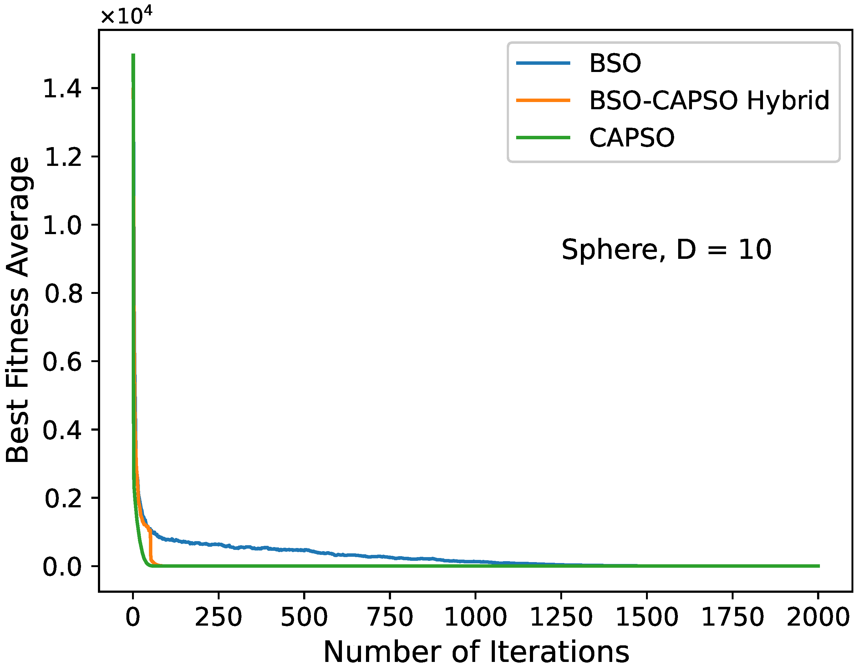
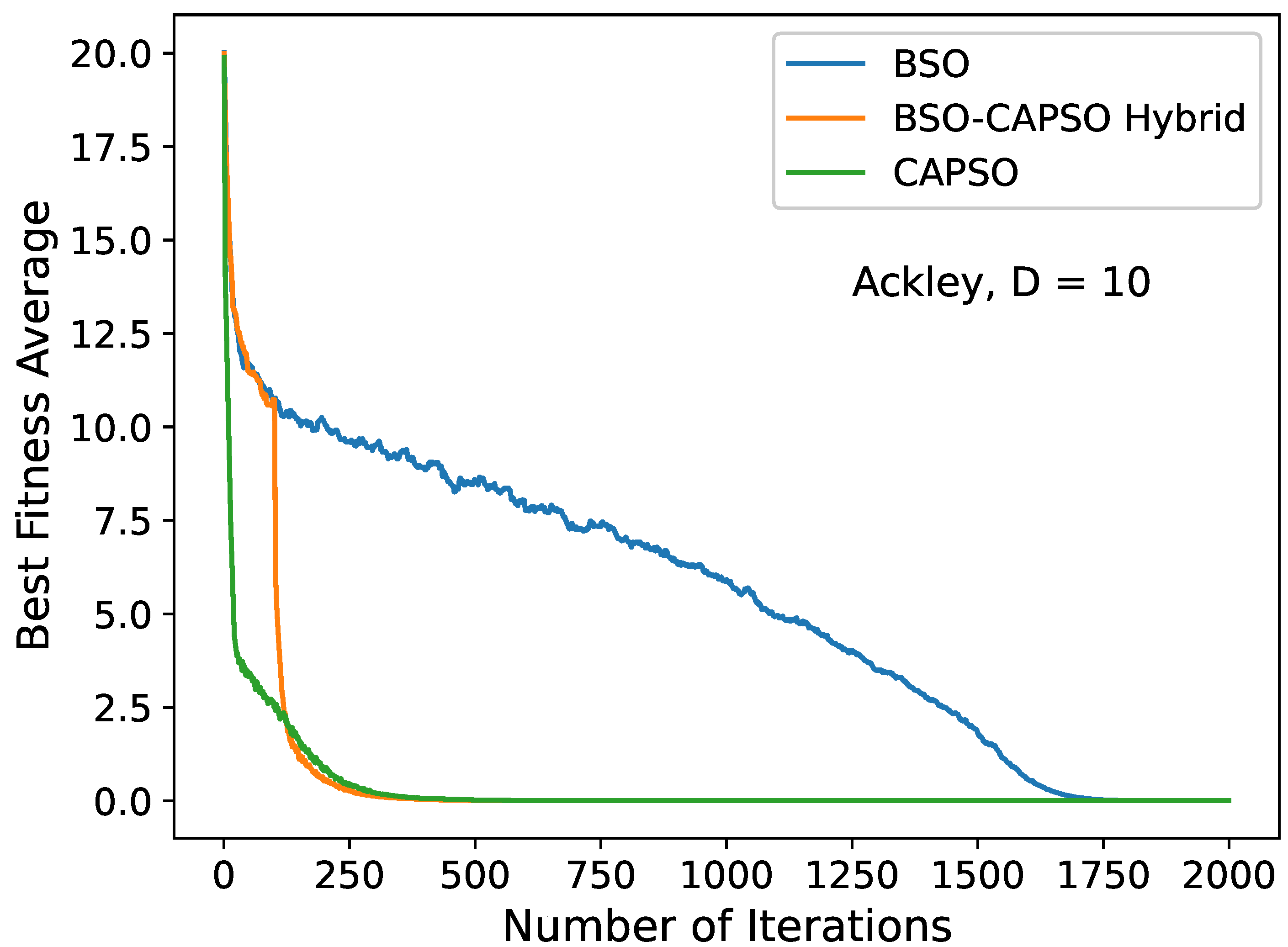
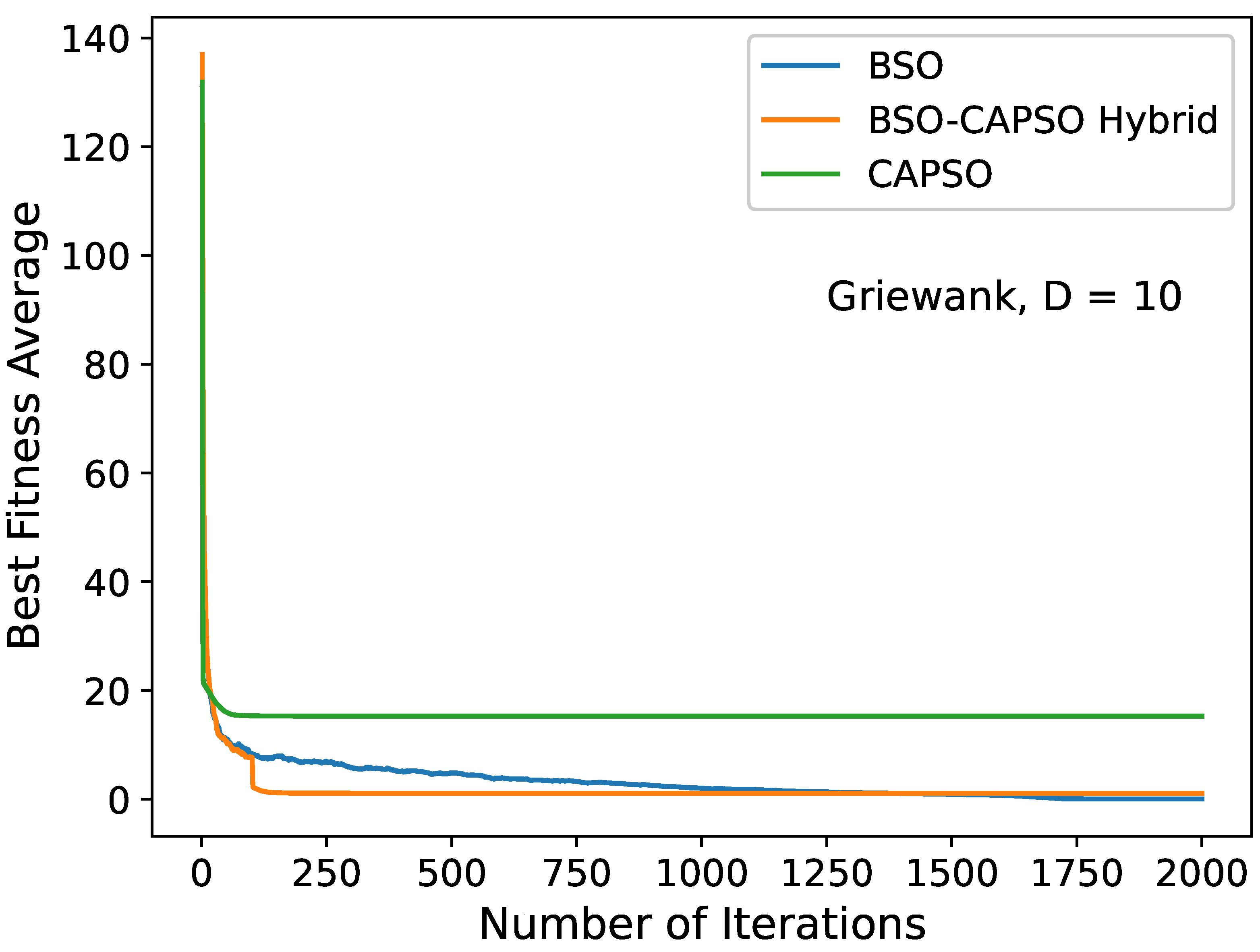
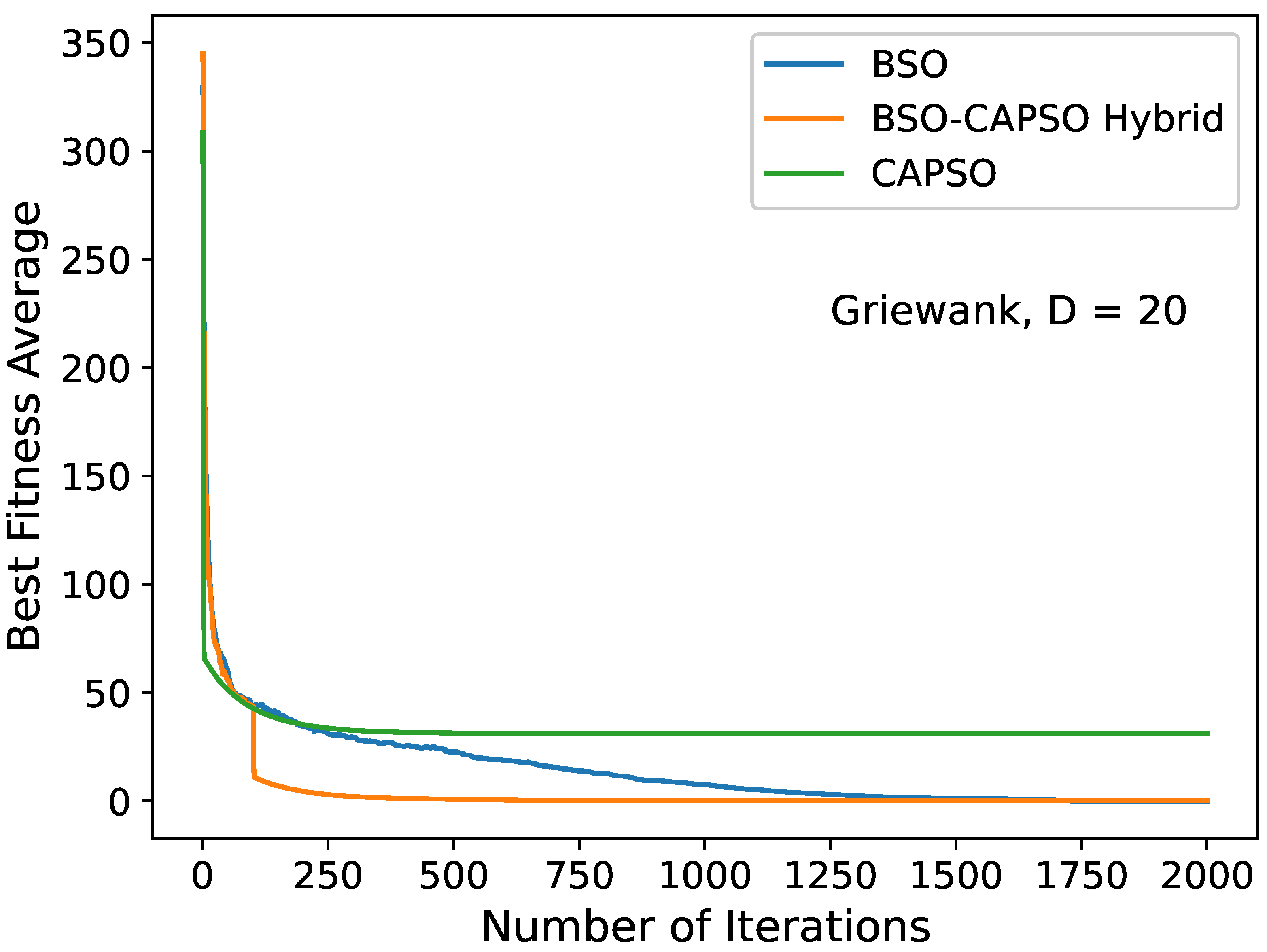
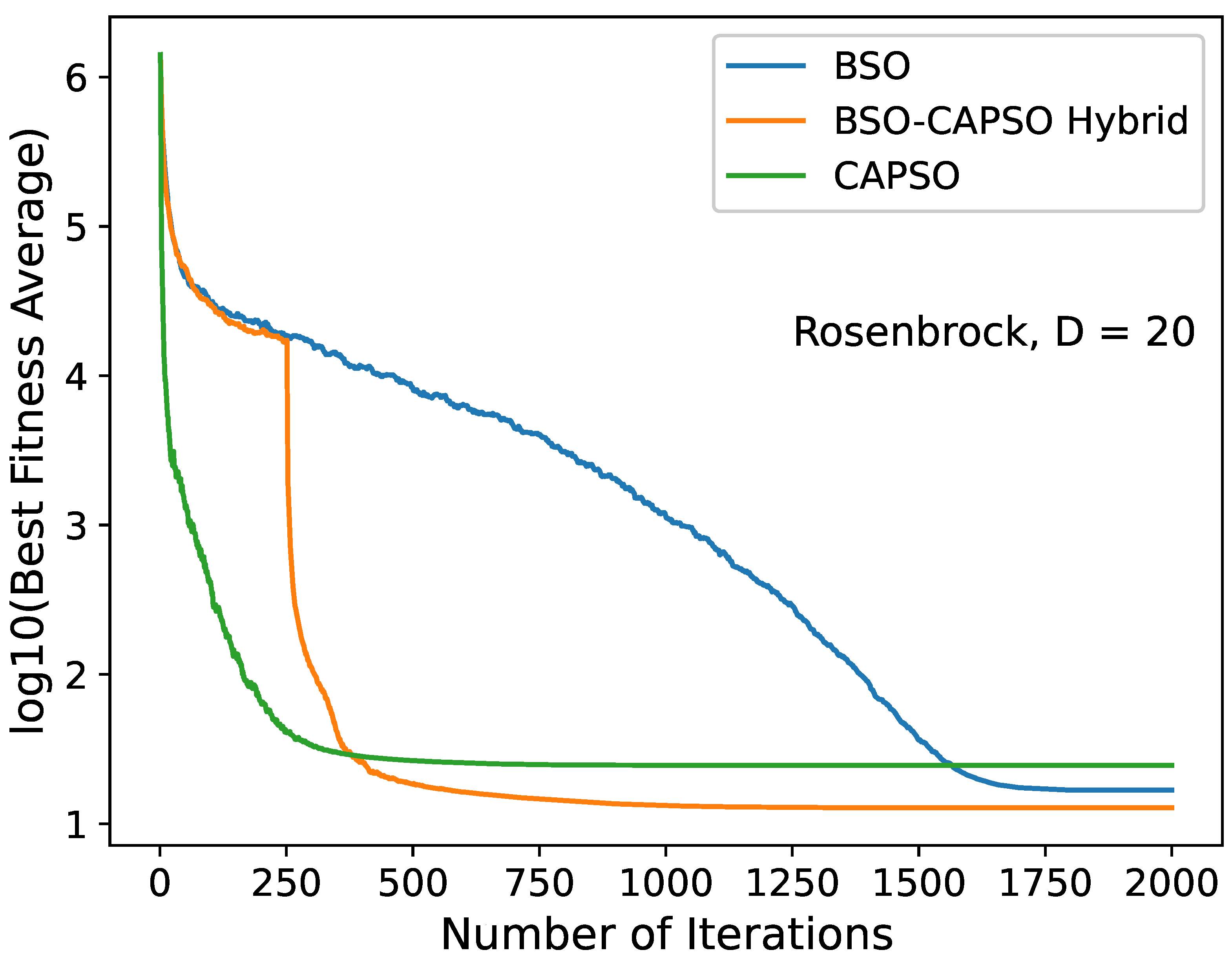
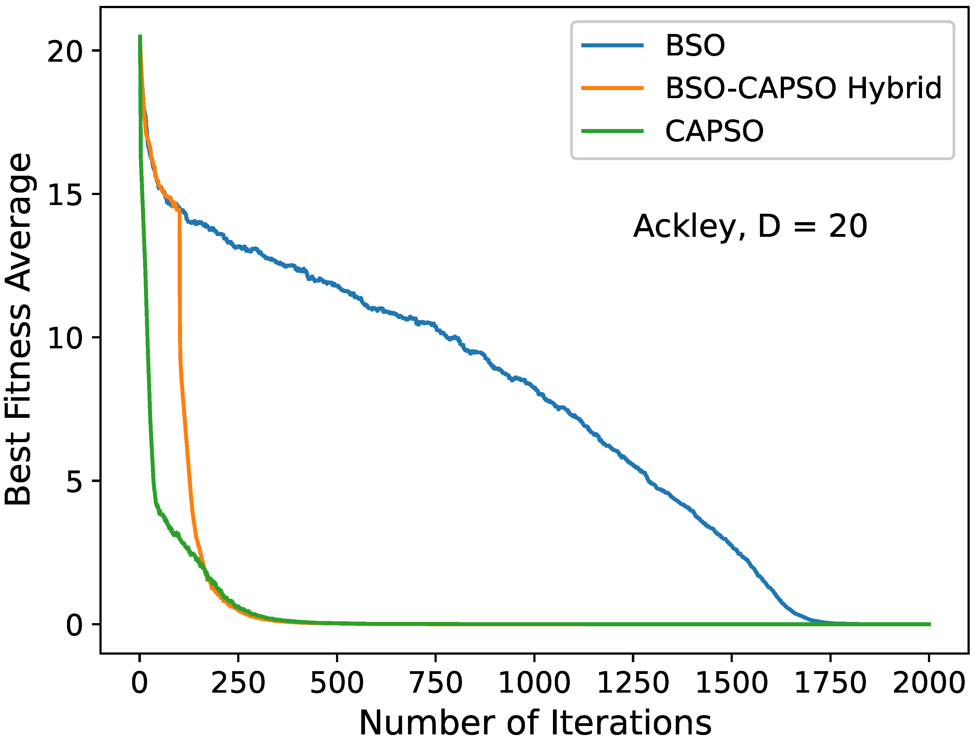
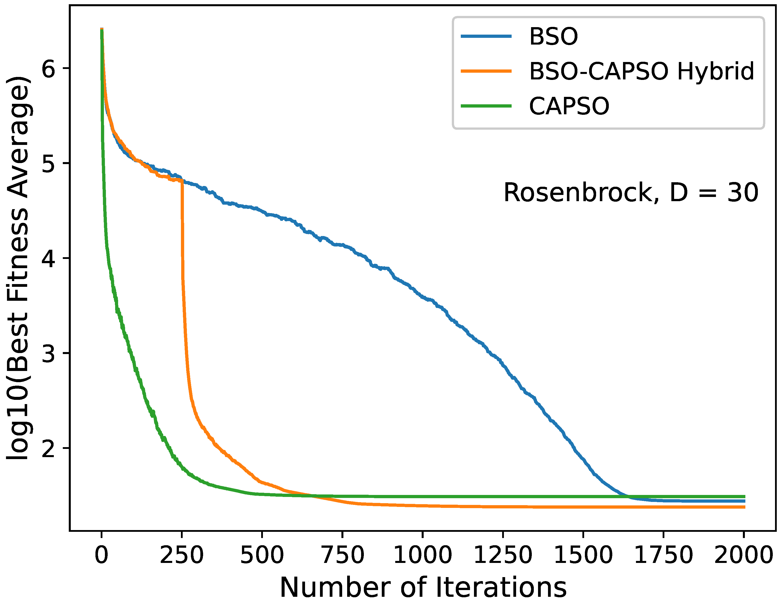
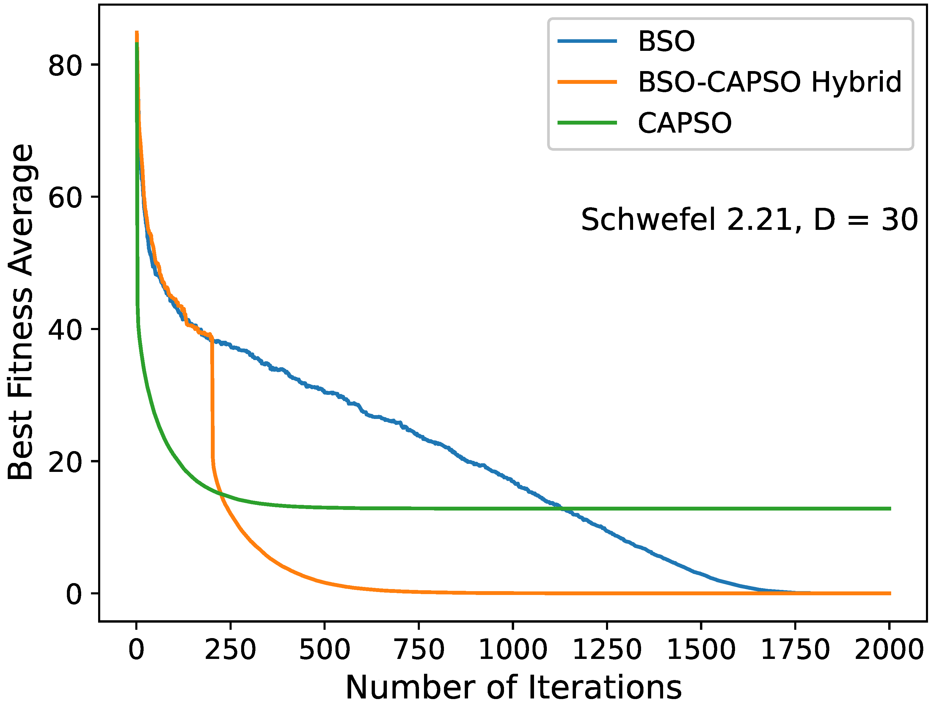
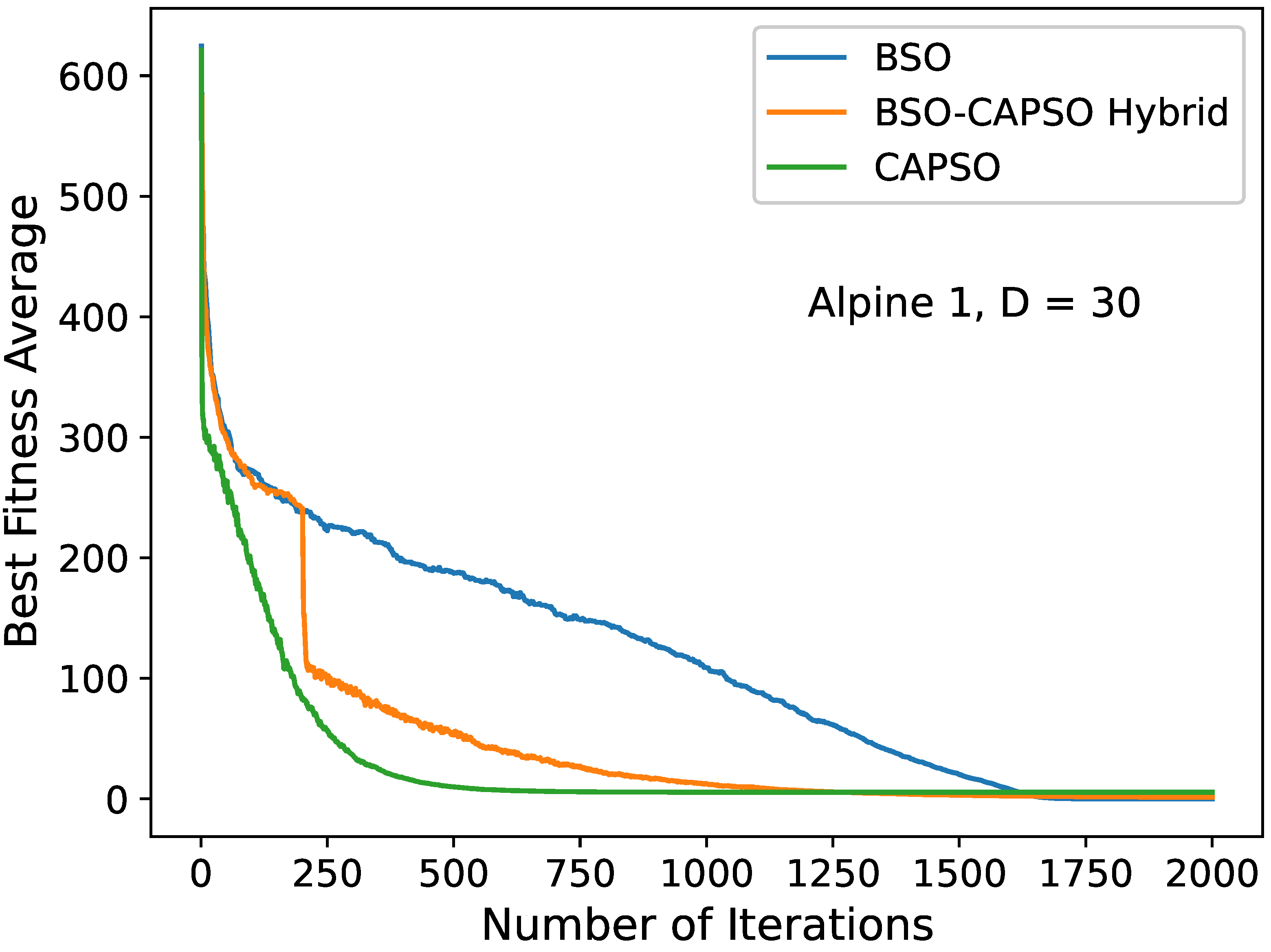
BSO–CAPSO was tested on seven benchmark functions of various characteristics for different numbers of dimensions. Results showed advantageous behavior when compared to stand-alone BSO and CAPSO. Particularly, the results provided demonstrated that the BSO–CAPSO hybrid achieved the following:
  • It severely outperformed CAPSO for most types of optimization benchmarks that were tested.
  • It was more effective when optimizing unimodal functions compared to BSO.
  • It showed advantageous behavior in multimodal problems with various degrees of success compared to BSO.
  • It was noticeably computationally lighter than BSO, to around one third of its computation time.
  • It led to high-quality local search areas within a short amount of iterations.
Thus, the BSO–CAPSO hybrid could be successfully used to explore areas of complex optimization problems efficiently and provide useful solutions or local search areas. It could improve both of the stand-alone algorithms, while its application was not of greater complexity.
The rest of the paper is outlined as follows. In Section 2, the theoretical bases of stand-alone BSO and CAPSO are presented in detail. In Section 3, we present the BSO–CAPSO hybrid as a concept; its parameters and hybridization method are demonstrated and explained. In Section 4, we expand on the experimental parameters and conditions while the benchmarking functions are also provided in detail. Information regarding the hybrid’s parameter tuning is provided alongside a detailed presentation of the parameters used for our set of experiments. In Section 5, the results for all the experiments are provided. The BSO–CAPSO hybrid is compared to the stand-alone BSO and CAPSO algorithms for all the benchmarking functions and for different numbers of dimensions. Computation time is also accounted for. The results are accompanied by several convergence diagrams to visualize the differences of the algorithms’ behaviors and efficiency. Finally, in Section 6, the observations regarding the results provided are organized and presented, and the benefits of the BSO–CAPSO hybrid are discussed. Additionally, further discussions regarding the applications of the proposed hybrid algorithm and future experimentation are included.

2. Background

2.1. Brain Storm Optimization (BSO)

BSO is inspired by the brainstorming process observed in groups of humans, which is generally characterized by a plethora of behaviors and mental processes. During brainstorming, a heterogeneous group of people tries to find solutions to a given problem. The group has the ability to generate new ideas, exchange information, inspire each other, form subgroups and constantly improve the candidate solution(s) formed within the group.
The algorithm modeling such a behavior was introduced by Shi in [10]. Precisely, a group of N people gathers to facilitate solutions to a difficult problem. Through the various interactions and dynamics, new ideas are generated with respect to Osborn’s four original laws of the brainstorming process [36]:
  • Suspend judgement: No idea can be denoted as good or bad. Judging too early is also advised against. The judgement of ideas is reserved for the end of the brainstorming process.
  • Anything goes: Any generated idea holds potential value, so every idea is presented to and shared with the group.
  • Cross-fertilize (piggyback): A plethora of ideas can come to life when an already existing idea is further explored and improved. Ideas themselves should be treated as generators of new ideas.
  • Go for quantity: It is of great importance to generate a very large number of ideas. Improved ideas come from other ideas, so quality depends on quantity for this concept and it will naturally emerge in time.

2.2. The BSO Algoritm

The original BSO algorithm has received various modifications to improve its effectiveness and adaptability to optimization problems. BSO, as it has been developed in this work, is described in the following steps.
  • Population initialization: As is common for evolutionary stochastic optimization, N points in a D-dimensional search space are randomly generated. In BSO, they are referred to as ideas. The initialization formula for the i t h idea is
    x i d = x m i n d + rand ( ) ( x m a x d x m i n d ) ,
    where d is one of the D dimensions and x m a x d , x m i n d are its maximum and minimum boundaries, respectively. The function rand ( ) returns a number between 0 and 1 via a uniform distribution.
  • Idea clustering: The N ideas are clustered into m groups, depending on their positions in the search space. Various clustering methods have been applied to and experimented with BSO. In this work, we used the k-means algorithm [10,37], which is the most popular. The variant applied to k-means is k-means++.
  • Idea evaluation: Each idea’s fitness is evaluated with respect to the objective function, f. The best idea in each one of the m clusters is denoted as the cluster center.
  • Cluster center disruption: This occasionally occurs to increase the population’s diversity. Disruption is controlled by the probability p r e p . A random number is generated. If this number is smaller than p r e p , one of the clusters is randomly selected and its center is replaced by a newly generated idea according to Equation (1).
  • Idea population update: The most important step in evolutionary global optimization algorithms is the update scheme. In BSO, a new idea can be generated from a chosen one. The update formula, see [10], is
    x n e w d = x c h o s e n d + ξ N ( 0 , 1 ) ,
    where N ( 0 , 1 ) is a Gaussian random value with mean 0 and variance 1. The original BSO algorithm [10] used a logarithmic sigmoid function for ξ , while alternative approaches were also developed [38,39,40]. In this work, see [14,33], ξ is calculated by
    ξ ( t ) = κ rand ( ) exp 1 T T t + 1 ,
    where T is the maximum number of iterations, t is the current iteration and κ adapts to the size of the search space as
    κ = 0.25 ( x m a x x m i n ) .
    The idea x c h o s e n can be a single selected idea from one cluster or a combination of two ideas from two clusters. This is similarly controlled by a probability, p g e n .
    (a)
    In one-cluster idea selection, a single cluster is selected. The probability of choosing a cluster is proportional to its size. After the cluster is chosen, x c h o s e n is either its center or a randomly chosen idea in it. This is controlled by p o n e C .
    (b)
    In two-cluster idea selection, two clusters are randomly chosen. The probability of choosing each cluster is the same. Similarly to one-cluster selection, either two centers or two random ideas are chosen. This is controlled by p t w o C . The two selected ideas are combined as
    x c h o s e n d = rand ( ) x s e l e c t e d 1 d + ( 1 rand ( ) ) x s e l e c t e d 2 d .
    Then, x c h o s e n d is used to generate a new idea by means of Equation (2). The newly generated idea is compared to the current idea, i. If it is evaluated as better, it replaces the current idea. Namely, for minimization problems, we have
    f ( x n e w ) < f ( x i ) : x i = x n e w ,
    while for maximization problems we have
    f ( x n e w ) > f ( x i ) : x i = x n e w .
    This iterative process takes place for all the individuals (ideas) in the population until the entire population has been updated for the cases when Equations (6) or (7) apply.
  • Termination criteria: Many termination criteria can be applied to BSO. One of the most common ones, and the one used in this paper, is when the maximum number of iterations T is reached. This mean that the population update process occurs T times.
Algorithm 1 contains simple pseudocode for the developed BSO.
Algorithm 1: BSO Algorithm
Algorithms 16 00208 i001

Clustering: k-Means Algorithm

In general, a clustering algorithm is presented with a set of objects (or data points) and groups them into clusters, meaning groups, according to the similarities they share. Clustering is a process met in many fields, such as data analysis, machine learning and pattern recognition. BSO utilizes clustering in order to group similar ideas (solutions) together. In BSO, ideas exist in the D-dimensional space of the optimization problem, thus similarity is examined as the distance between them in that space.
The k-means algorithm is a clustering algorithm that groups objects according to their Euclidean distance with respect to the space they belong in [41]. It forms groups around centers (centroids), which are the same in number as the number of clusters needed, and keeps refining them according to their distances from the iteratively updated centroids. Basic pseudocode for the k-means clustering process is presented in Algorithm 2.
In the k-means++ variant of the algorithm [42], the process is exactly the same except for the consideration of more refined sampling during the centroid initialization phase in order to speed up convergence. Particularly, it initializes the centroids to be adequately distant from each other, leading to (probably) better results than random initialization.
Algorithm 2: k-means Algorithm
Algorithms 16 00208 i002
It should be emphasized that the centroid of the k-means or k-means++ algorithm is not related to the cluster center we referred to in the BSO algorithm. The centroid is not necessarily a member of the population, it is a point in space that serves as a center and a point of reference. On the other hand, the cluster center is defined after the clusters are obtained as the solution with the fittest objective function evaluation.

2.3. Chaotic Accelerated Particle Swarm Optimization (CAPSO)

The original PSO algorithm [15,16] is inspired by the swarm intelligence observed in the behavior of swarms of birds in search for food. Swarms of birds (and other species, e.g., schools of fish) have the ability to cooperate instead of compete in order to find food sources. The members of the swarm have the ability to maintain cohesion, alignment and separation, while they also exhibit cognitive behaviors. They have memory for their own past success during the exploration process, while they can also communicate useful information to each other regarding food allocation.
Usually, in PSO algorithms, we do not refer to animals, but particles, meaning points (vectors) in the D-dimensional solution space. Each particle, i, represents a member of the swarm with position x i and velocity v i , both being vectors of R D . In the original PSO algorithm, each particle takes into account both the global best position, g , and its individual (local) best position, x i * , when it updates its velocity, v i .
The updated velocity is then used to update the position x i . So, the update scheme of PSO is performed in two steps.
The accelerated PSO (APSO) algorithm was proposed by Yang in 2008 [21,22]. Since the individual best of PSO is mainly used for necessary diversity, in the APSO algorithm this is instead simulated by randomness. Additionally, in APSO, each particle’s position updates in a single step (contrasting the two steps of PSO) as follows:
x n e w , i d = ( 1 β ) x i d + β g d + α N ( 0 , 1 ) ,
where β , commonly taken in [ 0.2 , 0.7 ] , is referred to as the attraction parameter for the global best and α , multiplied by a probability distribution, offers useful randomness to the updates. Here, a Gaussian random distribution is chosen. Moreover, it has been shown that a decreasing α is beneficial for the algorithm since, in this manner, it controls the exploration–exploitation trade-off more adequately during the iterative process. To this end, a strictly-decreasing function, α ( t ) , was chosen, with a commonly used one being
α ( t ) = γ t ,
where γ ( 0 , 1 ) is a control parameter and t refers to time (the current iteration). It is important to fine-tune α ( t ) to the nature of the optimization problem and search area [17,21,22].
The chaotic APSO (CAPSO) [17] is a variant of the APSO algorithm. In the CAPSO algorithm, the same single-step routine with APSO is utilized (i.e., Equation (8)), but a varying β is deemed beneficial for improved performance. This global attraction parameter is updated through a chaotic map. In [17], many chaotic maps were tested, and the most advantageous results stemmed from the sinusoidal and singer maps. Here, a simplified sinusoidal map was chosen for β , particularly
β k + 1 = sin ( π β k ) , β 0 = 0.7 .
Algorithm 3 contains simple pseudocode for CAPSO.
Algorithm 3: CAPSO Algorithm
Algorithms 16 00208 i003

3. The BSO–CAPSO Hybrid Concept

The BSO–CAPSO hybrid approach is fairly simple. Since BSO has better initial exploration compared to PSO [33], we can safely assume that this could be similar for CAPSO. Additionally, if CAPSO is provided with a predetermined initialization (which is practically a form of information exploitation), it could potentially converge to even better solutions than PSO, since it favors acceleration and exploitation.
Thus, the proposed hybrid algorithm randomly initializes its population, and it first runs as BSO for a fixed number of iterations. When this number of iterations is reached, it continues the optimization process as CAPSO, taking the last BSO updated population as its “initial” population, meaning that the CAPSO phase is active for the remaining iterations. It is worth mentioning that CAPSO is easy to implement and less computationally heavy than BSO, which uses clustering. Hence, the BSO–CAPSO hybrid is expected to demand less computation time than stand-alone BSO.
Important parameters: We refer to the iteration during which the switch between algorithms occurs as t s w i t c h ; this parameter depends on the optimization problem. The guideline for selecting an advantageous t s w i t c h is to approximately choose an iteration during which BSO starts to favor exploration less and begins to favor exploitation more. This could be observed in convergence diagrams or determined through some sampling procedure.
Furthermore, α ( t ) of the CAPSO phase is crucial since it affects a great part of CAPSO’s exploration–exploitation behavior. CAPSO’s α ( t ) and BSO’s ξ ( t ) are, after all, the functions that also represent the exploration–exploitation trade-off of their respective algorithms and they need to be adequately synchronized for the hybrid. The CAPSO phase of the BSO–CAPSO hybrid begins with α ( t s w i t c h ) . Since the initial exploration is carried out by BSO, α ( t ) must be adjusted to the optimization problem in a way that when the switch happens the value α ( t s w i t c h ) is as follows:
  • Not too large (too much added diversity), meaning CAPSO would not take advantage of BSO’s initial exploration.
  • Not too small (too little added diversity), meaning CAPSO would greatly favor exploitation too early and possibly become trapped in a local minimum and not be able to escape.
As with stand-alone APSO/CAPSO, it is recommended to investigate and fine-tune the decreasing function α ( t ) versus the optimization problem’s characteristics, as well as t s w i t c h .
Clustering management: It is also important to note that since BSO utilizes the k-means (k-means++) algorithm, the results of the clustering process need to be appropriately managed. If there is some converging behavior during the BSO process of the hybrid, there is a possibility that the clustering algorithm returns with less clusters than the ones set as its parameter. In the hybrid algorithm’s developed code, we implemented simple mechanisms that always check the cluster number returned by the k-means algorithm and we adjusted the probabilities of cluster/idea picking accordingly so that the algorithm never chooses an empty cluster or nonexistent solution and, thus, fails.
Boundary enforcement: There exist many methods to ensure that candidate solutions remain within the lower and upper boundaries of the available D-dimensional space; indicatively, we refer to [43,44]. In this iteration of the hybrid BSO–CAPSO algorithm, the technique we applied was absorbing walls. This technique is quite straightforward: if a boundary is crossed, the value of the stray variable becomes the minimum (or maximum) value allowed, depending on which boundary is crossed. For the i t h idea/solution, if there is boundary crossing in the d t h dimension, the rule is enforced as follows (for the lower and upper boundary, respectively):
x i d < x m i n d : x i d = x m i n d
x i d > x m a x d : x i d = x m a x d
A simple technique was chosen since the examined benchmark functions were all of a different nature. In general, when an algorithm is applied to an open or complex problem, it is preferable to choose boundary conditions that cooperate sufficiently with the problem’s characteristics and constraints.
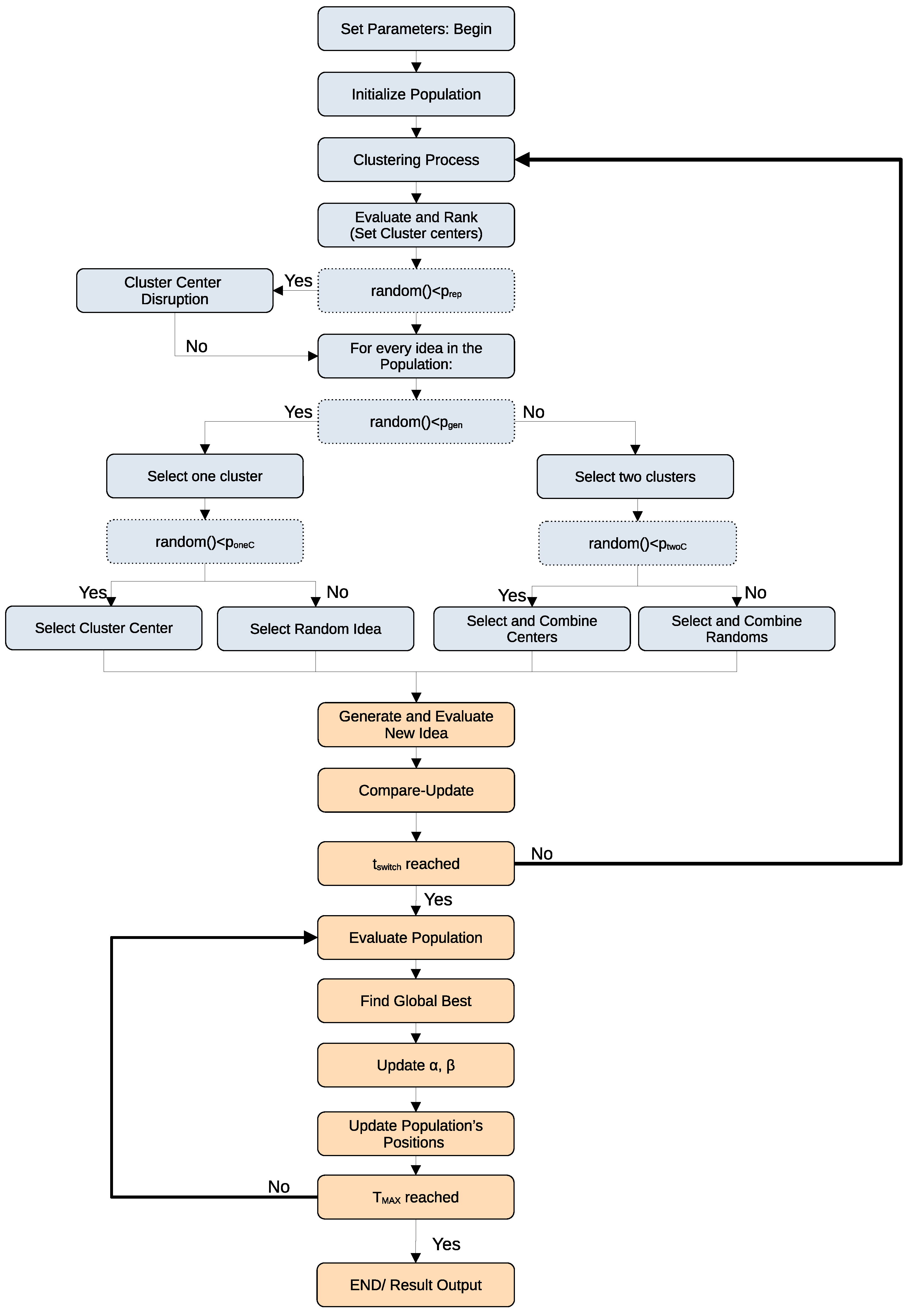
A flowchart diagram of the BSO–CAPSO hybrid algorithm is presented in Figure 1.

4. Considerations and Setup for the Numerical Experimentation

The BSO–CAPSO hybrid and stand-alone BSO/CAPSO algorithms were tested using the same benchmark functions to showcase the advantages of the hybrid approach.
It is noted that in this work, the proposed hybrid was compared to its parental algorithms; this is a fairly common practice, as can be seen in, e.g., [26,29,33], or similarly when a developed variant is examined against the main algorithm and/or closely-related variants [17,39,40,45].
BSO and PSO are very popular algorithms and their advantages and disadvantages are well documented. Moreover, CAPSO shares the same family tree with its main parental algorithm, PSO. Additionally, for CAPSO it has been demonstrated that it serves as an improvement to APSO and that it outperforms chaotic PSO (CPSO) [17]. Based on these considerations, the BSO–CAPSO hybrid is specifically examined as an improved alternative to the use of stand-alone BSO or CAPSO.

4.1. Benchmark Functions

Benchmark functions are typically used for testing optimization algorithms; Yang’s proposed test functions are widely utilized [46], while a recently organized collection is presented in [47]. In this work, we selected the functions f k presented in Table 1. Specifically, functions f 1 , f 2 , f 3 are unimodal, while functions f 4 , f 5 , f 6 , f 7 are multimodal.
In related works, the benchmarking experimentation process of an optimization algorithm has been examined in various manners. The original BSO [10] was initially only tested on two functions. In the hybrids presented in [27,29,32,33], the proposed algorithms were tested on two or three complex problems or designs in order to be evaluated. In this work, the above collection of seven popular functions served as an efficient and reliable experimental basis, with our approach being similar to [17,45], where six popular benchmarking functions were selected and examined. It is also important to note that multimodal functions are usually significantly more complex to optimize than unimodal ones. For this reason, more multimodal than unimodal functions were selected.

4.2. Experimental Parameters and Conditions

The stand-alone BSO, CAPSO and BSO–CAPSO hybrid algorithms were developed with Python3, with all experiments executed in the same computational platform. The employed k-means clustering algorithm was the one included in the scikit-learn library [48], which by default uses the k-means++ variant.
For each test, each algorithm was run 25 distinct times, for a maximum number of iterations T = 2000 , and the size of the population, N, was set as 4 D + 1 for D = 10 , 20 , 30 , yielding N = 41 , 81 , 121 , respectively. The numbers of clusters were set as one fifth or less of the population sizes, as is recommended in Ref. [14], thus m = 8 , 16 , 24 , respectively.

4.2.1. BSO Parameters

Both for the stand-alone BSO and the BSO–CAPSO hybrid, p r e p = 0.2 , p g e n = 0.8 , p o n e C = 0.4 and p t w o C = 0.5 , as suggested by BSO parameter selection studies [49].

4.2.2. CAPSO Parameters

For α ( t ) , we used Equation (9). We set the parameter γ as γ = 0.99 in order to be similar and comparable to the parameters chosen for the BSO–CAPSO hybrid.

4.2.3. BSO–CAPSO Hybrid Parameters

For the CAPSO phase, the β parameter updated through Equation (10). Additionally, its values were normalized in [ 0.2 , 0.7 ] [17]. For α ( t ) , we used Equation (9). Through experimentation, we noticed that values of γ 0.99 were the most beneficial. To produce such values, we used the following formula (a similar approach can be found in Ref. [50]):
γ = ( 10 20 ) 1 c T ,
where c > 0 , for which values of c ( 1 , 7.5 ) were adequate. It is also recommended to increase and adjust γ using (13) if the dimensions of the optimization problem increase. The adjusted t s w i t c h and the γ values per benchmark function f k are shown in Table 2. We note that if t s w i t c h was chosen somewhere between 2.5 % and 20 % of the number of iterations, T, the hybrid provided adequate solutions. The following t s w i t c h values were chosen with BSO’s behavior and the optimization problem’s complexity in mind.
We note that parameter tuning was applied while considering performance, but also stability. In general, stochastic algorithms, such as the ones employed in this paper, have a chance of providing outlier results, or results of varying orders of magnitude; this could be seen in BSO’s behavior for f 6 , f 7 , or the hybrid’s results for f 6 , as presented in Table 3. During the process of parameter selection, the hybrid provided outlier-like results for some parameter sets ( t s w i t c h and γ ). This was more probable in multimodal functions or functions with broader search areas when the parameters were not adequate. The provided sets of parameters and results were chosen with algorithm stability in mind, and each set of 25 algorithm runs was handled as a unit, a nonseparable experiment. It is also noted that for an acceptably wide range of parameter sets, outlier results were seldom and comparable to typical stochastic/metaheuristic algorithm behavior.

5. Results

The simulation results are given in Table 4 and Table 5 and they are organized per the number of dimensions, D. The results obtained were the mean, best and worst functions’ values, as well as average computation times (referred to as time), in seconds.

5.1. Time Calculations

In order to determine the computation time/cost for each experiment, Python 3’s library, Time (specifically time.perf_counter()), was used to calculate the difference between the moments in time an experiment began and ended. The signaling of an experiment’s beginning and ending remained exactly the same for each experiment, so that the results were as accurate as possible. All the experiments were performed on the same personal computer (CPU-AMD Ryzen 5 1600, RAM-8,00GB @ 1197MHz, OS-Windows 10 Pro 64-bit).

5.2. Convergence Diagrams

In Figure 2, Figure 3, Figure 4, Figure 5, Figure 6, Figure 7, Figure 8, Figure 9 and Figure 10, we depict certain convergence diagrams. Particularly, we plotted the average global best value of the considered benchmark function per iteration to provide some visual representations of the BSO–CAPSO hybrid’s behavior versus that of the BSO and CAPSO algorithms. The dimensions D = 10, 20 and 30 were considered. It was evident that the hybrid algorithm successfully accelerated convergence after t s w i t c h , while, simultaneously, it maintained the quality of the solutions compared to stand-alone BSO. It severely improved CAPSO. It specifically seemed to converge (or otherwise “accelerate”) more efficiently than CAPSO, while also improving the quality of its solutions in the vast majority of cases, especially regarding the complex multimodal functions. The diagrams’ data were obtained by the provided detailed results in Table 4 and Table 5.

6. Discussion and Conclusions

6.1. Observations and Remarks

The results demonstrated that the BSO–CAPSO Hybrid showcased improved behaviors compared to the stand-alone BSO and CAPSO algorithms. The hybrid provided better solutions regarding all unimodal functions, compared to both BSO and CAPSO. The only exception to this was the Schwefel 2.21 function, f 3 , for D = 10 dimensions, where CAPSO offered the best results. However, for larger numbers of dimensions the hybrid severely outperformed CAPSO for the said benchmark. For multimodal functions, the results were less absolute, but they were in favor of the hybrid approach. The hybrid outperformed CAPSO for all multimodal functions—with the exception of the Ackley function, f 5 , only for D = 30. In some cases, this was very impactful, such as for the Griewank function, f 6 . Compared to BSO it showcased both more and less advantageous results. Nevertheless, it decreased BSO’s computational time significantly— up to a third or less—while providing acceptable and comparable results. Additionally, the BSO–CAPSO hybrid accelerated convergence at t s w i t c h . This means that the BSO initialization could, indeed, be beneficial for CAPSO’s local exploitation. Additionally, acceleration at t s w i t c h often showcases the ability to discover a high-quality local search area (a high-quality attraction basin) very early during the iterative process, which means access to high-quality solutions with minimal computational costs; see, e.g., Figure 3 and Figure 6.
Moreover, it was observed that in some functions (e.g., f 3 , f 4 , f 6 ) discovering a good value for γ of α ( t ) (cf. Equation (9)) was challenging and demanded some intuition and a trial-and-error approach. This possibly implies that a different α ( t ) function could be more beneficial for these cases, since this function is also problem-dependent to some degree. In this work, however, guidelines regarding the tuning of the hybrid’s parameters were provided; thus, a solid baseline regarding parameter setting was solidified. Good results were obtained, and they supported the usage of the hybrid approach. Hence, it is also implied that the BSO–CAPSO’s performance on multimodal functions could be further improved; this was also discussed in Section 2.2 and Section 2.3, above. Future investigation into α ( t ) could benefit not only the BSO–CAPSO hybrid but also CAPSO’s use of hybridization in general. Additionally, although the sinusoidal chaotic map was showcased as the top performer in previous research regarding CAPSO [17], it is possible that different chaotic maps could be beneficial for some problems and should be considered in the BSO–CAPSO hybridization.

6.2. Further Discussion

Since BSO–CAPSO outperformed BSO significantly when applied to unimodal functions, we can assume that this hybrid approach could be efficiently utilized for local search in combination with global search optimization algorithms when applied to complex problems. If BSO–CAPSO is provided with a single attraction basin, or a small number of attraction basins, the results of this paper imply that it could outperform stand-alone BSO and provide a better result faster. This could extend to several multimodal functions, since the hybrid provided optimal results in some cases.
Regarding CAPSO, the hybrid approach demonstrated significant improvements compared to the stand-alone version, so it is advantageous to propose replacing CAPSO with the BSO–CAPSO hybrid when it is applied to a complex problem.
An important point of discussion is that several optimization problems remain open, very complex and computationally heavy (e.g., engineering optimization problems such as antenna design). In such problems, calculating the value of the objective function for a single solution or a set of solutions can be a time-consuming process. This means that the process of optimization through a metaheuristic global optimization method (which traditionally evaluates the objective function several hundreds or thousands of times) can be very computationally demanding. Thus, the use of the proposed hybrid could be applicable and valuable for such cases. This is reinforced if the BSO–CAPSO hybrid is applied to classes of problems that are known to benefit from BSO or algorithms with similar behaviors and effectiveness. Furthermore, when the global best solution of the problem is unknown, and, instead, the goal of the global optimization is a solution that serves specific quality conditions and constraints, BSO–CAPSO could prove fairly valuable since it is noticeably less time consuming and it shows a tendency to discover high-quality local search areas after t s w i t c h , which is a point early in the iterative process. Even in case of a potential loss of accuracy (when compared to standalone BSO), BSO–CAPSO could be an advantageous trade-off if solutions of the desired quality are obtained in a significantly smaller amount of computational time. Finally, the hybrid’s ability to discover high-quality local search areas early on is also promising for the future use of CAPSO hybridization, regarding the acceleration of optimization algorithms that utilize clustering or computationally heavy topologies for their exploration.

Author Contributions

Investigation, A.M. and N.L.T.; methodology, A.M. and N.L.T.; writing—review and editing, A.M. and N.L.T. All authors have read and agreed to the published version of the manuscript.

Funding

This research received no external funding.

Data Availability Statement

Data supporting reported results are available from the authors upon reasonable request.

Conflicts of Interest

The authors declare no conflict of interest.

Abbreviations

The following abbreviations were used in this manuscript:
PSOparticle swarm optimization;
BSObrain storm optimization;
APSOaccelerated particle swarm optimization;
CAPSOchaotic accelerated particle swarm optimization.

References

  1. Fister, I., Jr.; Yang, X.S.; Fister, I.; Brest, J.; Fister, D. A brief review of nature-inspired algorithms for optimization. arXiv 2013, arXiv:1307.4186. [Google Scholar]
  2. Tzanetos, A.; Dounias, G. Nature inspired optimization algorithms or simply variations of metaheuristics? Artif. Intell. Rev. 2021, 54, 1841–1862. [Google Scholar] [CrossRef]
  3. Vikhar, P.A. Evolutionary algorithms: A critical review and its future prospects. In Proceedings of the 2016 International Conference on Global Trends in Signal Processing, Information Computing and Communication (ICGTSPICC), Jalgaon, India, 22–24 December 2016; pp. 261–265. [Google Scholar] [CrossRef]
  4. Yang, X.S. Nature-inspired optimization algorithms: Challenges and open problems. J. Comput. Sci. 2020, 46, 101104. [Google Scholar] [CrossRef] [Green Version]
  5. Das, S.; Abraham, A.; Konar, A. Particle swarm optimization and differential evolution algorithms: Technical analysis, applications and hybridization perspectives. In Advances of Computational Intelligence in Industrial Systems; Springer: Berlin/Heidelberg, Germany, 2008; pp. 1–38. [Google Scholar]
  6. Ghamisi, P.; Benediktsson, J.A. Feature selection based on hybridization of genetic algorithm and particle swarm optimization. IEEE Geosci. Remote Sens. Lett. 2014, 12, 309–313. [Google Scholar] [CrossRef] [Green Version]
  7. Jadhav, A.N.; Gomathi, N. WGC: Hybridization of exponential grey wolf optimizer with whale optimization for data clustering. Alex. Eng. J. 2018, 57, 1569–1584. [Google Scholar] [CrossRef]
  8. Shelokar, P.; Siarry, P.; Jayaraman, V.K.; Kulkarni, B.D. Particle swarm and ant colony algorithms hybridized for improved continuous optimization. Appl. Math. Comput. 2007, 188, 129–142. [Google Scholar] [CrossRef]
  9. Teng, Z.j.; Lv, J.l.; Guo, L.w. An improved hybrid grey wolf optimization algorithm. Soft Comput. 2019, 23, 6617–6631. [Google Scholar] [CrossRef]
  10. Shi, Y. Brain storm optimization algorithm. In Proceedings of the International Conference in Swarm Intelligence, Chongqing, China, 14–15 June 2011; Springer: Berlin/Heidelberg, Germany, 2011; pp. 303–309. [Google Scholar]
  11. Cheng, S.; Sun, Y.; Chen, J.; Qin, Q.; Chu, X.; Lei, X.; Shi, Y. A comprehensive survey of brain storm optimization algorithms. In Proceedings of the 2017 IEEE Congress on Evolutionary Computation (CEC), San Sebastian, Spain, 5–8 June 2017; pp. 1637–1644. [Google Scholar] [CrossRef]
  12. Oliva, D.; Elaziz, M.A. An improved brainstorm optimization using chaotic opposite-based learning with disruption operator for global optimization and feature selection. Soft Comput. 2020, 24, 14051–14072. [Google Scholar] [CrossRef]
  13. Tuba, E.; Dolicanin, E.; Tuba, M. Chaotic brain storm optimization algorithm. In Proceedings of the International Conference on Intelligent Data Engineering and Automated Learning, Guilin, China, 30 October–1 November 2017; Springer: Cham, Switzerland, 2017; pp. 551–559. [Google Scholar] [CrossRef]
  14. Aldhafeeri, A.; Rahmat-Samii, Y. Brain Storm Optimization for Electromagnetic Applications: Continuous and Discrete. IEEE Trans. Antennas Propag. 2019, 67, 2710–2722. [Google Scholar] [CrossRef]
  15. Kennedy, J.; Eberhart, R. Particle swarm optimization. In Proceedings of the ICNN’95-International Conference on Neural Networks, Perth, WA, Australia, 27 November–1 December 1995; Volume 4, pp. 1942–1948. [Google Scholar] [CrossRef]
  16. Shi, Y.; Eberhart, R.C. Parameter selection in particle swarm optimization. In Proceedings of the International Conference on Evolutionary Programming, San Diego, CA, USA, 25–27 March 1998; Springer: Berlin/Heidelberg, Germany, 1998; pp. 591–600. [Google Scholar] [CrossRef]
  17. Gandomi, A.H.; Yun, G.J.; Yang, X.S.; Talatahari, S. Chaos-enhanced accelerated particle swarm optimization. Commun. Nonlinear Sci. Numer. Simul. 2013, 18, 327–340. [Google Scholar] [CrossRef]
  18. Michaloglou, A.; Tsitsas, N.L. Feasible Optimal Solutions of Electromagnetic Cloaking Problems by Chaotic Accelerated Particle Swarm Optimization. Mathematics 2021, 9, 2725. [Google Scholar] [CrossRef]
  19. Michaloglou, A.; Tsitsas, N.L. Particle Swarm Optimization Algorithms with Applications to Wave Scattering Problems. In Optimisation Algorithms and Swarm Intelligence; IntechOpen Limited: London, UK, 2021. [Google Scholar] [CrossRef]
  20. Zhou, Q.; Zhang, W.; Cash, S.; Olatunbosun, O.; Xu, H.; Lu, G. Intelligent sizing of a series hybrid electric power-train system based on Chaos-enhanced accelerated particle swarm optimization. Appl. Energy 2017, 189, 588–601. [Google Scholar] [CrossRef]
  21. Yang, X.S. Engineering Optimization: An Introduction with Metaheuristic Applications; John Wiley & Sons: Hoboken, NJ, USA, 2010. [Google Scholar]
  22. Yang, X.S. Nature-Inspired Optimization Algorithms; Academic Press: Cambridge, MA, USA, 2020. [Google Scholar]
  23. Narmatha, C.; Eljack, S.M.; Tuka, A.A.R.M.; Manimurugan, S.; Mustafa, M. A hybrid fuzzy brain-storm optimization algorithm for the classification of brain tumor MRI images. J. Ambient. Intell. Humaniz. Comput. 2020, 1–9. [Google Scholar] [CrossRef]
  24. Ibrahim, R.A.; Abd Elaziz, M.; Ewees, A.A.; Selim, I.M.; Lu, S. Galaxy images classification using hybrid brain storm optimization with moth flame optimization. J. Astron. Telesc. Instruments Syst. 2018, 4, 038001. [Google Scholar] [CrossRef]
  25. Bezdan, T.; Zivkovic, M.; Bacanin, N.; Chhabra, A.; Suresh, M. Feature Selection by Hybrid Brain Storm Optimization Algorithm for COVID-19 Classification. J. Comput. Biol. 2022, 29, 515–529. [Google Scholar] [CrossRef]
  26. Alzaqebah, M.; Jawarneh, S.; Alwohaibi, M.; Alsmadi, M.K.; Almarashdeh, I.; Mohammad, R.M.A. Hybrid brain storm optimization algorithm and late acceptance hill climbing to solve the flexible job-shop scheduling problem. J. King Saud-Univ.-Comput. Inf. Sci. 2022, 34, 2926–2937. [Google Scholar] [CrossRef]
  27. Hua, Z.; Chen, J.; Xie, Y. Brain storm optimization with discrete particle swarm optimization for TSP. In Proceedings of the 2016 12th International Conference on Computational Intelligence and Security (CIS), Wuxi, China, 16–19 December 2016; pp. 190–193. [Google Scholar]
  28. Kao, Y.T.; Zahara, E. A hybrid genetic algorithm and particle swarm optimization for multimodal functions. Appl. Soft Comput. 2008, 8, 849–857. [Google Scholar] [CrossRef]
  29. Juang, C.F. A hybrid of genetic algorithm and particle swarm optimization for recurrent network design. IEEE Trans. Syst. Man Cybern. Part B Cybern. 2004, 34, 997–1006. [Google Scholar] [CrossRef]
  30. Thangaraj, R.; Pant, M.; Abraham, A.; Bouvry, P. Particle swarm optimization: Hybridization perspectives and experimental illustrations. Appl. Math. Comput. 2011, 217, 5208–5226. [Google Scholar] [CrossRef]
  31. Sengupta, S.; Basak, S.; Peters, R.A. Particle Swarm Optimization: A survey of historical and recent developments with hybridization perspectives. Mach. Learn. Knowl. Extr. 2018, 1, 157–191. [Google Scholar] [CrossRef] [Green Version]
  32. Victoire, T.A.A.; Jeyakumar, A.E. Hybrid PSO–SQP for economic dispatch with valve-point effect. Electr. Power Syst. Res. 2004, 71, 51–59. [Google Scholar] [CrossRef]
  33. Song, L.; Rahmat-Samii, Y. Hybridizing Particle Swarm and Brain Storm Optimizations for Applications in Electromagnetics. In Proceedings of the 2021 XXXIVth General Assembly and Scientific Symposium of the International Union of Radio Science (URSI GASS), Rome, Italy, 28 August–4 September 2021; pp. 1–4. [Google Scholar] [CrossRef]
  34. Alkayem, N.F.; Cao, M.; Shen, L.; Fu, R.; Šumarac, D. The combined social engineering particle swarm optimization for real-world engineering problems: A case study of model-based structural health monitoring. Appl. Soft Comput. 2022, 123, 108919. [Google Scholar] [CrossRef]
  35. Alkayem, N.F.; Shen, L.; Al-hababi, T.; Qian, X.; Cao, M. Inverse Analysis of Structural Damage Based on the Modal Kinetic and Strain Energies with the Novel Oppositional Unified Particle Swarm Gradient-Based Optimizer. Appl. Sci. 2022, 12, 11689. [Google Scholar] [CrossRef]
  36. Smith, R. The 7 Levels of Change: Diffferent Thinking for Diffferent Results; Tapestry Press: Abingdon, UK, 2002; Volume 3. [Google Scholar]
  37. Zhu, H.; Shi, Y. Brain storm optimization algorithms with k-medians clustering algorithms. In Proceedings of the 2015 Seventh International Conference on Advanced Computational Intelligence (ICACI), Wuyi, China, 27–29 March 2015; pp. 107–110. [Google Scholar] [CrossRef]
  38. Cao, Z.; Hei, X.; Wang, L.; Shi, Y.; Rong, X. An improved brain storm optimization with differential evolution strategy for applications of ANNs. Math. Probl. Eng. 2015, 2015, 923698. [Google Scholar] [CrossRef] [Green Version]
  39. El-Abd, M. Brain storm optimization algorithm with re-initialized ideas and adaptive step size. In Proceedings of the 2016 IEEE Congress on Evolutionary Computation (CEC), Vancouver, BC, Canada, 24–29 July 2016; pp. 2682–2686. [Google Scholar] [CrossRef]
  40. Zhou, D.; Shi, Y.; Cheng, S. Brain storm optimization algorithm with modified step-size and individual generation. In Proceedings of the International Conference in Swarm Intelligence, Shenzhen, China, 17–20 June 2012; Springer: Berlin/Heidelberg, Germany, 2012; pp. 243–252. [Google Scholar] [CrossRef]
  41. Lloyd, S. Least squares quantization in PCM. IEEE Trans. Inf. Theory 1982, 28, 129–137. [Google Scholar] [CrossRef] [Green Version]
  42. Vassilvitskii, S.; Arthur, D. k-means++: The advantages of careful seeding. In Proceedings of the Eighteenth Annual ACM-SIAM Symposium on Discrete Algorithms, San Diego, CA, USA, 22–24 January 2006; pp. 1027–1035. [Google Scholar]
  43. Wang, D.; Tan, D.; Liu, L. Particle swarm optimization algorithm: An overview. Soft Comput. 2018, 22, 387–408. [Google Scholar] [CrossRef]
  44. Huang, T.; Mohan, A.S. A hybrid boundary condition for robust particle swarm optimization. IEEE Antennas Wirel. Propag. Lett. 2005, 4, 112–117. [Google Scholar] [CrossRef] [Green Version]
  45. Li, L.; Zhang, F.; Chu, X.; Niu, B. Modified brain storm optimization algorithms based on topology structures. In Proceedings of the Advances in Swarm Intelligence: 7th International Conference, ICSI 2016, Bali, Indonesia, 25–30 June 2016; pp. 408–415. [Google Scholar]
  46. Yang, X.-S. Test problems in optimization. arXiv 2010, arXiv:1008.0549. [Google Scholar]
  47. Plevris, V.; Solorzano, G. A Collection of 30 Multidimensional Functions for Global Optimization Benchmarking. Data 2022, 7, 46. [Google Scholar] [CrossRef]
  48. Pedregosa, F.; Varoquaux, G.; Gramfort, A.; Michel, V.; Thirion, B.; Grisel, O.; Blondel, M.; Prettenhofer, P.; Weiss, R.; Dubourg, V.; et al. Scikit-learn: Machine Learning in Python. J. Mach. Learn. Res. 2011, 12, 2825–2830. [Google Scholar]
  49. Zhan, Z.H.; Chen, W.N.; Lin, Y.; Gong, Y.J.; Li, Y.L.; Zhang, J. Parameter investigation in brain storm optimization. In Proceedings of the 2013 IEEE Symposium on Swarm Intelligence (SIS), Singapore, 16–19 April 2013; pp. 103–110. [Google Scholar] [CrossRef]
  50. Yang, X.S.; Accelerated Particle Swarm Optimization (APSO). Online at MATLAB Central File Exchange. 2022. Available online: https://www.mathworks.com/matlabcentral/fileexchange/74766-accelerated-particle-swarm-optimization-apso (accessed on 1 April 2022).
Figure 1. Flowchart diagram of the BSO–CAPSO hybrid algorithm.
Algorithms 16 00208 g001
Figure 2. Convergence diagram of the stand-alone BSO, BSO–CAPSO hybrid and stand-alone CAPSO algorithms for the sphere ( f 1 ) function with D = 10 . Convergence acceleration occurred after t s w i t c h = 50 .
Algorithms 16 00208 g002
Figure 3. Convergence diagram of the stand-alone BSO, BSO–CAPSO hybrid and CAPSO algorithms for the Ackley ( f 5 ) function with D = 10 . Convergence acceleration occurred after t s w i t c h = 100 .
Algorithms 16 00208 g003
Figure 4. Convergence diagram of the stand-alone BSO, BSO–CAPSO hybrid and CAPSO algorithms for the Griewank ( f 6 ) function with D = 10 . Convergence acceleration occurred after t s w i t c h = 100 .
Algorithms 16 00208 g004
Figure 5. Convergence diagram of the stand-alone BSO, BSO–CAPSO hybrid and stand-alone CAPSO algorithms for the Griewank ( f 6 ) function with D = 20 . Convergence acceleration occurred after t s w i t c h = 100 .
Algorithms 16 00208 g005
Figure 6. Convergence diagram of the stand-alone BSO, BSO–CAPSO hybrid and stand-alone CAPSO algorithms for the Rosenbrock ( f 2 ) function with D = 20 . Convergence acceleration occurred after t s w i t c h = 250 .
Algorithms 16 00208 g006
Figure 7. Convergence diagram of the stand-alone BSO, BSO–CAPSO hybrid and stand-alone CAPSO algorithms for the Ackley ( f 5 ) function with D = 20 . Convergence acceleration occurred after t s w i t c h = 100 .
Algorithms 16 00208 g007
Figure 8. Convergence diagram of the stand-alone BSO, BSO–CAPSO hybrid and stand-alone CAPSO algorithms for the Rosenbrock ( f 2 ) function with D = 30 . Convergence acceleration occurred after t s w i t c h = 250 .
Algorithms 16 00208 g008
Figure 9. Convergence diagram of the stand-alone BSO, BSO–CAPSO hybrid and stand-alone CAPSO algorithms for the Schwefel 2.21 ( f 3 ) function with D = 30 . Convergence acceleration occurred after t s w i t c h = 200 .
Algorithms 16 00208 g009
Figure 10. Convergence diagram of the stand-alone BSO, BSO–CAPSO hybrid and stand-alone CAPSO algorithms for the Alpine 1 ( f 7 ) function with D = 30 . Convergence acceleration occurred after t s w i t c h = 200 .
Algorithms 16 00208 g010
Table 1. Benchmark functions.
FunctionFormulaGlobal MinimumSearch Area
Sphere f 1 = i = 1 D x i 2 f 1 ( x * ) = 0 , x * = { 0 , , 0 } [ 100 , 100 ] D
Rosenbrock f 2 = i = 1 D 1 [ 100 ( x i + 1 x i 2 ) 2 + ( 1 x i ) 2 ] f 2 ( x * ) = 0 , x * = { 1 , , 1 } [ 10 , 10 ] D
Schwefel 2.21 f 3 = max i = 1 , , D | x i | f 3 ( x * ) = 0 , x * = { 0 , , 0 } [ 100 , 100 ] D
Rastrigin f 4 = 10 D + i = 1 D [ x i 2 10 cos ( 2 π x i ) ] f 4 ( x * ) = 0 , x * = { 0 , , 0 } [ 5.12 , 5.12 ] D
Ackley f 5 = 20 exp 0.2 1 D n = 1 D x i 2 exp 1 D i = 1 D cos 2 π x i + e + 20 f 5 ( x * ) = 0 , x * = { 0 , , 0 } [ 32.768 , 32.768 ] D
Griewank f 6 = 1 4000 i = 1 D x i 2 i = 1 D cos x i i + 1 f 6 ( x * ) = 0 , x * = { 0 , , 0 } [ 600 , 600 ] D
Alpine 1 f 7 = i = 1 D | x i sin ( x i ) + 0.1 x i | f 7 ( x * ) = 0 , x * = { 0 , , 0 } [ 100 , 100 ] D
Table 2. BSO–CAPSO hybrid parameter values per benchmark function.
D = 10D = 20D = 30
t switch γ t switch γ t switch γ
f 1 500.9817479430199844500.9885530946569389500.9885530946569389
f 2 2500.99235409613210052500.99294016136668182500.9934427784709274
f 3 2000.99166191953867642000.99426007395295672000.9958222329003689
f 4 4000.99472068575697704000.99478052112557794000.9948099330498242
f 5 1000.98855309465693891000.98922280011554641000.9902907258434653
f 6 1000.98855309465693891000.99540541735152701000.9967159968972744
f 7 2000.99426007395295672000.99582223290036892000.9967159968972744
Table 3. Simulation results for D = 10.
BSOBSO–CAPSO HybridCAPSO
D : 10 MeanBestWorstTimeMeanBestWorstTimeMeanBestWorstTime
f 1 5.08 × 10 14 2.69 × 10 15 2.50 × 10 13 99.955.59 × 10 32 3.30 × 10 32 1.17 × 10 31 13.201.92 × 10 17 6.95 × 10 18 3.22 × 10 17 11.44
f 2 5.74 × 10 0 4.08 × 10 0 6.48 × 10 0 105.971.70 × 10 0 5.03 × 10 2 5.53 × 10 0 23.873.22 × 10 0 0.34 × 10 0 7.92 × 10 0 12.53
f 3 2.92 × 10 6 3.14 × 10 7 1.01 × 10 5 97.457.35 × 10 8 5.08 × 10 8 1.05 × 10 7 19.072.72 × 10 9 1.85 × 10 9 3.54 × 10 9 10.74
f 4 4.38 × 10 0 9.95 × 10 1 7.96 × 10 0 109.469.55 × 10 0 1.99 × 10 0 1.89 × 10 1 34.761.65 × 10 1 4.97 × 10 0 3.28 × 10 1 13.88
f 5 7.34 × 10 8 9.34 × 10 9 2.45 × 10 7 116.023.03 × 10 10 1.83 × 10 10 5.08 × 10 10 18.845.52 × 10 9 3.38 × 10 9 7.44 × 10 9 14.74
f 6 4.0 × 10 2 7.40 × 10 3 9.60 × 10 2 116.701.09 × 10 0 3.71 × 10 1 1.98 × 10 0 20.881.53 × 10 1 7.98 × 10 0 2.61 × 10 1 15.22
f 7 7.05 × 10 8 1.21 × 10 8 4.52 × 10 7 114.813.97 × 10 2 3.17 × 10 4 2.64 × 10 1 24.311.13 × 10 0 2.04 × 10 7 6.87 × 10 0 13.41
Table 4. Simulation results for D = 20.
BSOBSO–CAPSO HybridCAPSO
D : 20 MeanBestWorstTimeMeanBestWorstTimeMeanBestWorstTime
f 1 2.17 × 10 10 2.53 × 10 11 1.28 × 10 9 187.461.93 × 10 19 1.10 × 10 19 3.40 × 10 19 45.746.11 × 10 17 3.65 × 10 17 8.17 × 10 17 42.72
f 2 1.68 × 10 1 1.55 × 10 1 1.76 × 10 1 213.091.28 × 10 1 9.90 × 10 0 1.70 × 10 1 68.542.46 × 10 1 1.25 × 10 1 1.52 × 10 2 48.19
f 3 1.57 × 10 4 5.84 × 10 5 5.05 × 10 4 185.892.05 × 10 5 1.42 × 10 5 2.62 × 10 5 55.294.53 × 10 0 3.96 × 10 9 1.37 × 10 1 40.49
f 4 1.32 × 10 1 6.96 × 10 0 1.89 × 10 1 224.781.91 × 10 1 9.95 × 10 0 3.88 × 10 1 85.314.66 × 10 1 3.18 × 10 1 8.36 × 10 1 53.41
f 5 2.91 × 10 6 1.18 × 10 6 5.00 × 10 6 230.731.49 × 10 9 1.08 × 10 9 1.93 × 10 9 61.737.46 × 10 9 5.57 × 10 9 9.95 × 10 9 54.26
f 6 3.15 × 10 3 3.97 × 10 10 2.22 × 10 2 246.621.56 × 10 1 9.75 × 10 9 1.38 × 10 0 68.863.12 × 10 1 9.77 × 10 0 5.01 × 10 1 59.24
f 7 1.25 × 10 4 1.37 × 10 6 1.79 × 10 3 260.693.72 × 10 1 3.63 × 10 2 1.42 × 10 0 68.832.70 × 10 0 1.42 × 10 1 1.32 × 10 1 51.48
Table 5. Simulation results for D = 30.
BSOBSO–CAPSO HybridCAPSO
D : 30 MeanBestWorstTimeMeanBestWorstTimeMeanBestWorstTime
f 1 4.88 × 10 9 8.11 × 10 10 1.95 × 10 8 313.013.75 × 10 19 2.38 × 10 19 5.95 × 10 19 99.641.38 × 10 16 8.92 × 10 17 2.18 × 10 16 92.19
f 2 2.77 × 10 1 2.69 × 10 1 2.86 × 10 1 347.052.39 × 10 1 2.08 × 10 1 2.92 × 10 1 137.793.08 × 10 1 2.18 × 10 1 1.25 × 10 2 108.55
f 3 9.99 × 10 4 3.75 × 10 4 2.25 × 10 3 288.036.10 × 10 4 5.02 × 10 4 7.65 × 10 4 110.771.28 × 10 1 6.48 × 10 0 2.06 × 10 1 89.58
f 4 2.22 × 10 1 9.95 × 10 0 3.38 × 10 1 379.653.64 × 10 1 1.59 × 10 1 6.27 × 10 1 167.258.45 × 10 1 3.58 × 10 1 1.50 × 10 2 118.06
f 5 1.51 × 10 5 6.73 × 10 6 2.20 × 10 5 375.911.48 × 10 8 1.13 × 10 8 1.89 × 10 8 130.918.30 × 10 9 6.99 × 10 9 9.47 × 10 9 119.61
f 6 1.25 × 10 6 8.74 × 10 8 4.41 × 10 6 419.781.91 × 10 2 3.42 × 10 6 7.60 × 10 2 145.276.72 × 10 1 3.55 × 10 1 9.58 × 10 1 129.30
f 7 1.67 × 10 3 3.03 × 10 5 4.73 × 10 3 390.751.24 × 10 0 3.77 × 10 1 2.54 × 10 0 142.585.46 × 10 0 5.94 × 10 1 1.34 × 10 1 114.90
Disclaimer/Publisher’s Note: The statements, opinions and data contained in all publications are solely those of the individual author(s) and contributor(s) and not of MDPI and/or the editor(s). MDPI and/or the editor(s) disclaim responsibility for any injury to people or property resulting from any ideas, methods, instructions or products referred to in the content.

