A Trajectory-Based Immigration Strategy Genetic Algorithm to Solve a Single-Machine Scheduling Problem with Job Release Times and Flexible Preventive Maintenance

Abstract

This paper considers the single-machine problem with job release times and flexible preventive maintenance activities to minimize total weighted tardiness, a complicated scheduling problem for which many algorithms have been proposed in the literature. However, the considered problems are rarely solved by genetic algorithms (GAs), even though it has successfully solved various complicated combinatorial optimization problems. For the problem, we propose a trajectory-based immigration strategy, where immigrant generation is based on the given information of solution extraction knowledge matrices. We embed the immigration strategy into the GA method to improve the population’s diversification process. To examine the performance of the proposed GA method, two versions of GA methods (the GA without immigration and the GA method with random immigration) and a mixed integer programming (MIP) model are also developed. Comprehensive experiments demonstrate the effectiveness of the proposed GA method by comparing the MIP model with two versions of GA methods. Overall, the proposed GA method significantly outperforms the other GA methods regarding solution quality due to the trajectory-based immigration strategy.

1. Introduction

In this paper, we consider the single-machine problem with job release times and machine unavailable periods, where machine unavailable periods are caused by flexible preventive maintenance (PM) activities. For classical single-machine scheduling problems, most research assumes that all jobs are ready for processing simultaneously or that machines are always available to simplify the complexity of scheduling problems. These two assumptions may impede many possible practical applications, and some studies have demonstrated that there is a need to consider the dynamic job release time [1] or machine unavailable periods [2,3]. Both are common phenomena in the real world and are significant factors in production scheduling decisions. That is, taking into consideration jobs’ release time and machine unavailable periods, a given production scheduling problem can be solved more realistically.

For the considered problem, more precisely, there are n jobs with different release times to the production system and waiting to be processed on a single machine without preemption. The machine is not always available; it needs to be maintained periodically to prevent its continuous working time from exceeding a specific threshold value and to initialize the machine’s status. To the best of our knowledge, there are only three studies considering dynamic job release time and machine availability constraints simultaneously for the single-machine scheduling problem. Detienne [4] was the first to consider this type of problem and proposed a MIP model to minimize the weighted number of late jobs. In this study, the machine unavailable periods were fixed and known in advance. Cui and Lu [5] considered the dynamic job release time for the machine availability scheduling problem. The main difference from the study of Detienne [4] is that, when implementing PM as a decision variable in scheduling planning, it is not fixed and known. For this problem, the researchers proposed a MIP model, heuristic algorithms and the branch and bound (BAB) method to minimize the makespan. Pang et al. [6] considered the single-machine maintenance scheduling problem with dynamic job release time, and this study was motivated by a clean operation of semiconductor manufacturing in which the machine had to stop to remove the dirt in the machine as a clean agent. For this problem, the researchers proposed a scatter simulated annealing algorithm to simultaneously minimize the total weighted tardiness and total completion time.

Our considered problem is the same as that of Cui and Lu [5] mentioned above; the objective of Cui and Lu [5] is to minimize the makespan, implying maximizing the throughput of the system. With the increasing importance of time-related competition and customer satisfaction, production performance based on due-dates becomes more significant. Thus, the objective we adopted is to minimize the total weighted tardiness (TWT) for responding to the needs of on-time delivery in just-in-time (JIT) production, which is one of the important, relevant objectives for today’s manufacturing environments. Moreover, the TWT objective has not been considered as often by researchers in this problem. This problem is also NP-hard because the special case without machine maintenance constraints, that is, the single-machine scheduling problem to minimize the total weighted tardiness has proven to be NP-hard [7].

For the NP-hard problem considered in this paper, we propose a trajectory-based immigration strategy genetic algorithm. The main reason is that different genetic algorithms (GAs) have been implemented successfully in many complicated scheduling problems but are seldom applied to the considered problem. Additionally, an immigration strategy is one of the common ways to keep the diversity of the population and avoid local convergence. Thus, we develop a novel trajectory-based immigration strategy containing three different solution knowledge extraction matrices for collecting important information from the searched chromosomes and embed the immigration strategy into the proposed GA method to generate better immigrants. Furthermore, we develop a mixed integer programming (MIP) model to obtain benchmark solutions to evaluate the performance of the proposed GA.

The rest of this paper is as follows. In Section 2, we review previous related studies. We define the considered problem and a mixed integer programming model to minimize the total weighted tardiness in Section 3. In Section 4, we describe the trajectory-based GA in this paper. Section 5 describes the computational experiment, including the parameter settings of the GA, test data generation scheme and experimental results. In Section 6, we discuss the results obtained. Finally, Section 7 contains our conclusions and future research.

2. Literature Review

Regarding scheduling problems with machine availability constraints, hundreds of contributions have been developed in the literature. Most of the machine availability is caused by preventive maintenance. Preventive maintenance (PM) is designed as a prior measure to reduce the probability of failure or degradation, and activating PM tasks in scheduling problems are usually classified into two categories: (i) PM tasks are performed at a fixed interval or within a time window or (ii) PM tasks are carried out depending on certain monitored conditions. Table 1 exhibits a brief review of work on single-machine scheduling problems with PM tasks based on the two categories. As seen from Table 1, the previous major studies focused on the first category with different objective functions. Additionally, Ma et al. [8] provided a detailed review and classification of papers that dealt with deterministic scheduling problems related to fixed PM tasks in different manufacturing shop floors. This information indicated increasing interest in studying this field over the past several decades.

The references most pertinent to our considered paper are Qi et al. [9], Sbihi and Varnier [2], and Cui and Lu [5]. In these studies, the PM task is driven by monitoring the current machine’s working time to ensure that it does not exceed a preset critical time threshold and to initialize the status of the machine. Qi et al. [9] proposed three heuristic algorithms and a branch and bound (BAB) method to minimize the total completion time. Sbihi and Varnier [2] considered the two categories mentioned in Table 1 and proposed the BAB method to minimize maximum tardiness. The two above studies assumed that all jobs were ready at time 0. Cui and Lu [5] first considered the dynamic case of jobs’ release time in the single-machine problem. They proposed a mixed integer programming (MIP), a BAB method and a heuristic algorithm to minimize the makespan.

Another PM task motivated by the wafer cleaning operation of a semiconductor manufacturing factory was proposed by Su and Wang [10], where a machine has to be maintained periodically so that the amount of dirt left on the machine does not exceed a preset critical dirt threshold. Su and Wang [10] developed a MIP, a dynamic programming-based heuristic algorithm to minimize the total absolute deviation of job completion times. Later, Su et al. [11] extended the single-machine problem to a parallel machine problem and developed a MIP model and three heuristic algorithms to minimize the number of tardy jobs. Pang et al. [6] extended the study of Su and Wang [10] to consider job release time and bicriteria (total weighted tardiness and job completion time). They proposed a scatter simulated annealing (SSA) algorithm to obtain nondominated solutions.

From Table 1, it is evident that our considered problem, i.e., the dynamic single-machine scheduling problem with PM tasks, where PM tasks are driven by the threshold value of the machine’s continuous working time and the total weighted tardiness as the objective, has not been studied so far. The considered problem is NP-hard since the static single-machine problem with the objective of the total weighted tardiness, where the machine is always available, has proven to be NP-hard [7]. For this kind of NP-hard problem, applying traditional methodologies, such as heuristic algorithms or exact algorithms, suffers either from solution effectiveness or computational efficiency. In recent years, various GAs based on global exploration and local exploitation search mechanisms, due to their flexibility, have been utilized more successfully than traditional approaches in solving NP-hard problems [12].

Table 1. Two categories of related studies for the considered problem.

Objectives	First Category	Second Category
Makespan	[3,13,14,15,16]	[5]
Total completion time or total flow time	[14,17,18,19,20]	[9]
Total weighted completion time	[21,22,23,24,25]	[26]
Total absolute deviation of job completion times		[10]
Maximum lateness	[14]	[26]
Maximum earliness	[27]
Maximum tardiness	[2,20,28]	[2]
Mean lateness	[20]
Mean tardiness	[20]
Number of tardy jobs	[14,29,30,31]	[11]
Weighted number of late jobs	[4]
Bicriteria (total weighted tardiness and total completion time)		[6]

Table 1. Two categories of related studies for the considered problem.

Objectives	First Category	Second Category
Makespan	[3,13,14,15,16]	[5]
Total completion time or total flow time	[14,17,18,19,20]	[9]
Total weighted completion time	[21,22,23,24,25]	[26]
Total absolute deviation of job completion times		[10]
Maximum lateness	[14]	[26]
Maximum earliness	[27]
Maximum tardiness	[2,20,28]	[2]
Mean lateness	[20]
Mean tardiness	[20]
Number of tardy jobs	[14,29,30,31]	[11]
Weighted number of late jobs	[4]
Bicriteria (total weighted tardiness and total completion time)		[6]

Compared with classical scheduling problems, employing meta-heuristic algorithms to solve single-machine scheduling problems with machine unavailability constraints has been very limited, with only a few studies to date. Pang et al. [6] considered a single-machine scheduling problem in which PM tasks are driven by the accumulated dirt and adopted the total weighted tardiness and total completion time simultaneously as an objective. The researchers proposed a scatter simulated annealing (SSA) algorithm to obtain nondominated solutions. Chen et al. [32] developed a GA to solve a single-machine scheduling problem by minimizing total tardiness, where machine availability is measured by its reliability. Due to their success in applying meta-heuristic algorithms to solve the scheduling problem with machine availability constraints, we propose a new GA with knowledge of solution trajectory, aiming at presenting a trajectory-based immigration strategy to enhance the effectiveness of our GA.

3. Problem Description and Methodology

3.1. Problem Description

Let J = {$J_j|$j = 1, 2, …, n} be the set of n jobs that are scheduled on a single machine. To keep the machine in good condition, the machine’s continuous working time cannot exceed a maximum specific time L. As a result, it is necessary to perform maintenance activity irregularly to initialize the machine. The maintenance time is MT. This paper considers non-preemptive and non-resumable cases; all jobs must be processed without interruption, and a job should be finished before a maintenance activity without restarting. Additionally, we assume that a job has a processing time, release time and due date for which data can be estimated in advance from the manufacturing execution system (MES). The objective is to minimize the total weighted tardiness (TWT) subject to the given job release time and maintenance constraint. According to the standard machine scheduling classification, the problem can be denoted as $1\left|r_j,nr,fpm\right|{\displaystyle \sum }{w}_j{T}_j$.

3.2. Mixed Integer Programming (MIP) Model

Based on the above description, we formulate a MIP model for the $1\left|r_j,nr, fpm\right|{\displaystyle \sum }{w}_j{T}_j$ problem. The parameters and variables used in the model are as follows:

• Parameters
  $n$: number of jobs
  $J_j$: job j
  $L$: maximum working time limit
  $MT$: maintenance time, which is a constant
  $M$: a very large positive integer constant
  $r_j$: release time of job j
  $p_j$: processing time of job j
  $w_j$: weight of job j
  $d_j$: due date of job j
• Decision variables
  $C_j$: completion time of job j
  $T_j$: tardiness of job j, where $T_j=max\left(0,C_j-d_j\right)$
  $X_{jk}$: 1 if job j is assigned at position k in the sequence, 0 otherwise
  $Y_k$: 1 if maintenance activity is assigned after position k in the sequence,
  0 otherwise
  $Q_k$: continuous working time of machine after position k in the sequence
  $S{T}_k$: start time at position k for processing in the sequence
  $P{T}_k$: processing time for the job assigned at position k in the sequence
  $C{T}_k$: completion time at position k in the sequence

To obtain a feasible schedule, variables $X_{jk}$ and $Y_k$ are binary and decide which job is assigned at position k and whether a maintenance activity is assigned after position k, as shown in Figure 1. This is based on the following constraints.

Each job must be arranged into exactly one position

$${{\displaystyle \sum }}_{k=1}^n{X}_{jk}=1\hspace{1em}\hspace{1em}\hspace{1em}\hspace{1em}\hspace{1em}\hspace{1em}\begin{array}{cc}\forall & j=1,2,3,\dots ,n\end{array}$$

(1)

Each position must be occupied by exactly one job

$${{\displaystyle \sum }}_{j=1}^n{X}_{jk}=1\hspace{1em}\hspace{1em}\hspace{1em}\hspace{1em}\hspace{1em}\hspace{1em}\begin{array}{cc}\forall & k=1,2,3,\dots ,n\end{array}$$

(2)

For each position k, the start time for the processing job can be given by

$$S{T}_k\ge {{\displaystyle \sum }}_{j=1}^n\left(r_j·X_{jk}\right)\hspace{1em}\hspace{1em}\hspace{1em}\hspace{1em}\hspace{1em}\begin{array}{cc}\forall & k=1,2,3,\dots ,n\end{array}$$

(3)

$$S{T}_k\ge C{T}_{k-1}+\left(MT·Y_{k-1}\right)\hspace{1em}\hspace{1em}\hspace{1em}\hspace{1em}\begin{array}{cc}\forall & k=2,3,4,\dots ,n\end{array}$$

(4)

For each position k, the processing time for the assigned job can be given by

$$P{T}_k={{\displaystyle \sum }}_{j=1}^n\left(p_j·X_{jk}\right)\hspace{1em}\hspace{1em}\hspace{1em}\hspace{1em}\hspace{1em}\begin{array}{cc}\forall & k=1,2,3,\dots ,n\end{array}$$

(5)

For each position k, the completion time of position k should be satisfied by

$$C{T}_k\ge S{T}_k+P{T}_k\hspace{1em}\hspace{1em}\hspace{1em}\hspace{1em}\hspace{1em}\hspace{1em}\begin{array}{cc}\forall & k=1,2,3,\dots ,n\end{array}$$

(6)

For the first position, the continuous working time can be given by

$$Q_1={{\displaystyle \sum }}_{j=1}^n\left(p_j·X_{j1}\right)$$

(7)

For each position k, excluding the first position, the continuous working time can be given by

$$Q_{k-1}+{{\displaystyle \sum }}_{j=1}^n\left(p_j·X_{jk}\right)\le Q_k+\left(M·Y_{k-1}\right)\hspace{1em}\hspace{1em}\begin{array}{cc}\forall & k=2,3,4,\dots ,n\end{array}$$

(8)

$${{\displaystyle \sum }}_{j=1}^n\left(p_j·X_{jk}\right)\le Q_k+M·\left(1-Y_{k-1}\right)\hspace{1em}\hspace{1em}\begin{array}{cc}\forall & k=2,3,4,\dots ,n\end{array}$$

(9)

In the above two equations, we apply the M value, a very large positive constant, to obtain the continuous working time for each position. If $Y_{k-1}=0$, then the continuous working time at position k ($Q_k$) will be forced to be $Q_{k-1}+{{\displaystyle \sum }}_{j=1}^n\left(p_j·X_{jk}\right)$; on the other hand, if $Y_{k-1}=1$, then the continuous working time at position k ($Q_k$) will be ${{\displaystyle \sum }}_{j=1}^n\left(p_j·X_{jk}\right)$.

For each position, the continuous working time should satisfy

$$Q_k\le L\hspace{1em}\hspace{1em}\hspace{1em}\hspace{1em}\hspace{1em}\hspace{1em}\hspace{1em}\begin{array}{cc}\forall & k=1,2,3,\dots ,n\end{array}$$

(10)

At the end of the sequence, there is no need to maintain the machine:

$$Y_n=0$$

(11)

For each job, the completion time can be given by

$$C_j+M·\left(1-X_{jk}\right)\ge C{T}_k\hspace{1em}\hspace{1em}\hspace{1em}\hspace{1em}\begin{array}{cc}\forall & \{\begin{array}{c}j=1,2,3,\dots ,n\\ k=1,2,3,\dots ,n\end{array}\end{array}$$

(12)

For each job, tardiness can be given by

$$T_j\ge \left(C_j-d_j\right)\hspace{1em}\hspace{1em}\hspace{1em}\hspace{1em}\hspace{1em}\hspace{1em}\begin{array}{cc}\forall & j=1,2,3,\dots ,n\end{array}$$

(13)

In this model, our goal is to minimize total weighted tardiness, which is given by

$$Min{{\displaystyle \sum }}_{j=1}^n(w_j·T_j)$$

(14)

It is worth noting from Figure 1 that the considered problem here involves two interrelated sets of decisions: how to sequence the jobs and when to execute PM activities. Implicitly, the decision of PM activities may affect the objective value, even for the same job sequence. To describe this phenomenon, suppose that the job sequence of J₁-J₃-J₄-J₅-J₂ is given for the 5-job instance in

Table 2. Five-job instance where L = 10 and MT = 5.

	${\mathit{r}}_{\mathit{j}}$	${\mathit{p}}_{\mathit{j}}$	${\mathit{d}}_{\mathit{j}}$	${\mathit{w}}_{\mathit{j}}$
$J_1$	0	2	4	1
$J_2$	8	8	17	3
$J_3$	5	2	9	2
$J_4$	7	4	12	2
$J_5$	13	4	19	3

, and two different PM decision methods are used for the job sequence.

The first PM decision method is inspired by the first fit (FF) concept for bin packing problems [33]. Thus, the jobs are assigned to the machine in orders as long as the working time of the machine does not exceed the threshold value (L). Based on the FF concept, the obtained TWT value is 51, according to the Gantt chart in Figure 2. The second PM decision method is motivated by the dynamic programming (DP) method for batch problems [34,35]. Using the DP method, the obtained TWT value is 41 to the Gantt chart in Figure 3. Additionally, the detailed steps of the DP method are demonstrated in Appendix A for the sake of brevity.

From this example, adopting the DP method as the PM decision method is better than the former. Moreover, the above two sets of decisions affect each other. In this paper, the sequence of jobs is in the form of chromosomes, and then the DP method is used as a decoding method to obtain an objective value for any chromosome in our GA.

4. The Proposed GA

GAs are well-known stochastic search algorithms to solve combinatorial optimization problems. The original idea was developed by Holland [36]. In a GA, a population is maintained by selection, crossover and mutation operators until a stopping criterion is satisfied and an optimal/best solution is obtained. However, it is likely to be trapped in local optima [37]. As a result, immigration strategies, such as random immigrants [38] and elitism-based immigrants [39], have been proposed to enhance the diversity of chromosomes in the population [40]. In this paper, we develop a trajectory-based immigrant scheme to maintain the diversity of chromosomes in each population.

Trajectory-based immigration schemes are not like random-based immigrant or elitism-based immigrant schemes. The former (random-based immigrant scheme) randomly generated immigrants. Regarding the latter, it adopted the elite chromosome as a base to generate immigrants with better solution quality in this way. In this paper, we develop a solution-characteristic reserved technology based on solution extraction knowledge matrices to extract the relation between job and position, job and job, and from job to job for each feasible solution. The solution extraction knowledge matrices are called job-position trajectory (JPT), job-job trajectory (JJT) and from-to trajectory (FTT). Based on the information provided by the three matrices, we develop a trajectory-based immigration scheme such that the generated immigrants can gain a balance between randomness and solution quality for the GA. Next, the steps for building three trajectory matrices are described as follows.

Step 1. Generate feasible schedules ${\pi }_y$ randomly and obtain the corresponding TWT value $x_y$, y = 1, 2, …, N. N is the number of the population.

Step 2. Calculate the mean ($\overline{x}={\displaystyle \sum }{x}_y/N$) and standard deviation ($\sigma =\sqrt{{\displaystyle \sum }{\left(x_y-\overline{x}\right)}^2/N-1}$) for this group.

Step 3. Obtain a semaphore value ($s_y$) for each schedule ${\pi }_y$ by normalization, i.e., $s_y=(\overline{x}-x_y)/\sigma$. Note that a larger signal is better to minimize the TWT.

Step 4. Initialize matrices CJP, CJJ, CFT, SJP, SJJ and SFT.

Step 5. Complete count matrix (CJP) by counting the number of jobs i occupied at position j in schedule ${\pi }_y$, and in a similar fashion to complete matrices (CJJ and CFT) if job i is before job j in schedule ${\pi }_y$, and if job i is from to job j (job i and j is adjacent).

Step 6. Complete semaphore matrix SJP by accumulating semaphore value ($s_y$) if job i occupied position j in schedule ${\pi }_y$, and in a similar fashion to complete matrix SJJ if job i is before job j in schedule ${\pi }_y$, and matrix SFT if from the job i is to job j.

Step 7. Obtain each element of the job-position trajectory (JPT) matrix by the following equation:

$$JP{T}_{ij}=\{\begin{array}{cc}0& if CJ{P}_{ij}=0\\ \frac{SJ{P}_{ij}}{CJ{P}_{ij}}& otherwise\end{array}\begin{array}{cc}\forall & \{\begin{array}{c}i=1,2,3,\dots ,n\\ j=1,2,3,\dots ,n\end{array}\end{array}$$

Step 8. Obtain each element of the job-job trajectory (JJT) matrix by the following equation:

$$JJ{T}_{ij}=\{\begin{array}{cc}0& if CJ{J}_{ij}=0\\ \frac{SJ{J}_{ij}}{CJ{J}_{ij}}& otherwise\end{array}\begin{array}{cc}\forall & \{\begin{array}{c}i=1,2,3,\dots ,n\\ j=1,2,3,\dots ,n\end{array}\end{array}$$

Step 9. Obtain each element of the from-to trajectory (FTT) matrix by the following equation:

$$FT{T}_{ij}=\{\begin{array}{cc}0& if CF{T}_{ij}=0\\ \frac{SF{T}_{ij}}{CF{T}_{ij}}& otherwise\end{array}\begin{array}{cc}\forall & \{\begin{array}{c}i=0,1,2,\dots ,n\\ j=0,1,2,\dots ,n\end{array}\end{array}$$

To demonstrate the three types of trajectory forms (job-position, job-job and from-to), we use an 8-job instance in

Table 3. Eight-job instance with L = 15 and MT = 5.

	${\mathit{J}}_1$	${\mathit{J}}_2$	${\mathit{J}}_3$	${\mathit{J}}_4$	${\mathit{J}}_5$	${\mathit{J}}_6$	${\mathit{J}}_7$	${\mathit{J}}_8$
$r_j$	35	45	44	33	41	3	32	43
$p_j$	8	13	3	5	3	3	4	3
$w_j$	3	1	7	2	8	3	1	3
$d_j$	47	55	62	44	56	16	49	58

and generate 1000 solutions randomly, for example. Applying the above steps, the JPT, JJT and FTT matrices are built, as shown in

Table 4. Job-position trajectory (JPT) matrix from 1000 random solutions for 8-job instance.

	Positions
		1	2	3	4	5	6	7	8
Jobs	1	0.31917	0.02314	−0.16659	−0.21222	−0.14115	−0.02065	0.06266	0.13564
	2	−1.38125	−0.79550	−0.41909	−0.10038	0.17369	0.46689	0.83788	1.21775
	3	−0.22808	0.20669	0.30798	0.26575	0.15107	−0.02584	−0.23395	−0.44361
	4	0.33685	0.00495	−0.12552	−0.11933	−0.08009	−0.21764	−0.46876	−0.71966
	5	0.25933	0.44942	0.41268	0.25655	0.02808	−0.21764	−0.46876	−0.71966
	6	0.87978	0.13539	−0.01647	−0.10382	−0.15826	−0.19973	−0.24555	−0.29134
	7	0.21466	−0.05454	−0.12392	−0.11331	−0.06601	−0.00804	0.04788	0.10329
	8	−0.40050	0.03045	0.13093	0.12675	0.09266	0.05228	0.00663	−0.03926

,

Table 5. Job-Job trajectory (JJT) matrix from 1000 random solutions for 8-job instance.

	Jobs
		1	2	3	4	5	6	7	8
Jobs	1	---	0.48009	−0.06691	−0.02260	−0.20985	−0.16732	0.00882	0.05005
	2	−0.48009	---	−0.53775	−0.48038	−0.70475	−0.62080	−0.43232	−0.40540
	3	0.06691	0.53775	---	0.00448	−0.12972	−0.08990	0.07447	0.09916
	4	0.02260	0.48038	−0.00448	---	−0.17715	−0.13956	0.02889	0.06497
	5	0.20985	0.70475	0.12972	0.17715	---	0.03882	0.20382	0.23131
	6	0.16732	0.62080	0.08990	0.13956	−0.03882	---	0.16483	0.19474
	7	−0.00882	0.43232	−0.07447	−0.02889	−0.20382	−0.16483	---	0.03258
	8	−0.05005	0.40540	−0.09916	−0.06497	−0.23131	−0.19474	−0.03258	---

and

Table 6. From-to trajectory (FTT) matrix from 1000 random solutions for an 8-job instance.

	To
		0	1	2	3	4	5	6	7	8
From	0	---	0.31917	−1.38125	−0.22808	0.33685	0.25933	0.87978	0.21466	−0.40045
	1	0.13564	---	0.18265	0.02463	−0.13640	−0.05755	−0.15306	−0.05853	0.06264
	2	1.21775	−0.25050	---	−0.08189	−0.19567	−0.27148	−0.27544	−0.11941	−0.02336
	3	−0.44361	0.02318	0.29617	---	0.00209	0.08335	−0.08437	−0.00576	0.12895
	4	0.03719	−0.10368	0.12910	0.02109	---	−0.02009	−0.09564	−0.01771	0.04974
	5	−0.71966	0.06846	0.39703	0.14226	0.02626	---	−0.06619	0.01413	0.13772
	6	−0.29134	0.03036	0.17156	0.02005	0.03065	−0.00769	---	0.01462	0.03179
	7	0.10329	−0.03578	0.07060	−0.00748	−0.01915	−0.03210	−0.09235	---	0.01297
	8	−0.03926	−0.05121	0.13414	0.10942	−0.04461	0.04624	−0.11273	−0.04199	---

.

To validate whether the three matrices can help us to find good immigrants, we applied correlation analysis to realize the correlation between the objective value and matrices. The steps are described as follows:

Step 1. For instance, generate K feasible solutions (π𝑦) randomly and obtain objective values ($x_y$) for solution y, y = 1, 2,…, K.

Step 2. For each solution, ${\pi }_y=\left\{J_{\left[1\right]}, J_{\left[2\right]},\dots J_{\left[i\right]},\dots ,J_{\left[j\right]},\dots ,J_{\left[n\right]}\right\}$, obtain three feature values based on the JPT, JJT and FTT matrices using the following equations:

$$Z{1}_y={{\displaystyle \sum }}_{j=1}^{n}JP{T}_{J_{\left[j\right]},j}$$

$$Z{2}_y={\displaystyle \sum }_{i=1}^{n-1}{{\displaystyle \sum }}_{j=i+1}^{n}JJ{T}_{J_{\left[i\right]},J_{\left[j\right]}}$$

$$Z{3}_y=FT{T}_{0, J_{\left[1\right]}}+{{\displaystyle \sum }}_{j=1}^{n-1}FT{T}_{J_{\left[j\right]},J_{\left[j+1\right]}}+FT{T}_{J_{\left[n\right]}, 0}$$

Step 3. Obtain the mean and standard deviation of the objective value and feature values for the K solutions using the following equations:

$$\overline{x}=\frac{1}{K}{{\displaystyle \sum }}_{y=1}^K{x}_y,S_x=\sqrt{{{\displaystyle \sum }}_{y=1}^K{\left(x_y-\overline{x}\right)}^2/\left(K-1\right)}$$

$$\overline{Z1}=\frac{1}{K}{{\displaystyle \sum }}_{y=1}^{K}Z{1}_y,S_{Z1}=\sqrt{{{\displaystyle \sum }}_{y=1}^K{\left(Z{1}_y-\overline{Z1}\right)}^2/\left(K-1\right)}$$

$$\overline{Z2}=\frac{1}{K}{{\displaystyle \sum }}_{y=1}^{K}Z{2}_y,S_{Z2}=\sqrt{{{\displaystyle \sum }}_{y=1}^K{\left(Z{2}_y-\overline{Z2}\right)}^2/\left(K-1\right)}$$

$$\overline{Z3}=\frac{1}{K}{{\displaystyle \sum }}_{y=1}^{K}Z{3}_y,S_{Z3}=\sqrt{{{\displaystyle \sum }}_{y=1}^K{\left(Z{3}_y-\overline{Z3}\right)}^2/\left(K-1\right)}$$

Step 4. Calculate the correlation values between the objective value and matrices by the following equation:

$$r_{x,Z1}=\frac{1}{\left(K-1\right)}\times {\displaystyle \sum }_{y=1}^K\left(\frac{x_y-\overline{x}}{S_x}\right)\times \left(\frac{Z{1}_y-\overline{Z1}}{S_{Z1}}\right)$$

$$r_{x,Z2}=\frac{1}{\left(K-1\right)}\times {\displaystyle \sum }_{y=1}^K\left(\frac{x_y-\overline{x}}{S_x}\right)\times \left(\frac{Z{2}_y-\overline{Z2}}{S_{Z2}}\right)$$

$$r_{x,Z3}=\frac{1}{\left(K-1\right)}\times {\displaystyle \sum }_{y=1}^K\left(\frac{x_y-\overline{x}}{S_x}\right)\times \left(\frac{Z{3}_y-\overline{Z3}}{S_{Z3}}\right)$$

For the example of Table 3 and based on the results in Table 4, Table 5 and Table 6, we determine that the correlation values $\left(r_{x,Z1}, r_{x,Z2}, r_{x,Z3}\right)$ are −0.97130, −0.88297 and −0.81809 when K = 250. The values are negative because the objective function is minimized. To further examine the correlation between objective value and matrices, we randomly regenerate 80 instances with eight jobs and follow the procedures mentioned above to obtain the correlation values shown in

Table 7. Obtained correlation values between the objective value and matrices for different instances.

No.	${\mathit{r}}_{\mathit{x},\mathit{Z}1}$	${\mathit{r}}_{\mathit{x},\mathit{Z}2}$	${\mathit{r}}_{\mathit{x},\mathit{Z}3}$	No.	${\mathit{r}}_{\mathit{x},\mathit{Z}1}$	${\mathit{r}}_{\mathit{x},\mathit{Z}2}$	${\mathit{r}}_{\mathit{x},\mathit{Z}3}$
1	−0.97398	−0.90259	−0.82521	41	−0.93246	−0.78268	−0.82146
2	−0.93389	−0.67382	−0.91551	42	−0.96903	−0.90456	−0.82889
3	−0.89515	−0.70715	−0.79133	43	−0.96012	−0.85805	−0.85599
4	−0.95873	−0.85844	−0.80679	44	−0.96275	−0.75995	−0.83542
5	−0.98988	−0.85009	−0.82317	45	−0.93506	−0.64075	−0.83282
6	−0.97103	−0.78600	−0.86143	46	−0.94614	−0.81629	−0.86377
7	−0.96237	−0.80414	−0.81064	47	−0.95039	−0.68591	−0.88292
8	−0.95706	−0.83210	−0.80263	48	−0.92468	−0.81150	−0.81777
9	−0.93486	−0.64478	−0.81466	49	−0.95806	−0.78674	−0.90038
10	−0.96672	−0.78058	−0.87700	50	−0.97217	−0.83153	−0.84326
11	−0.95342	−0.73581	−0.86859	51	−0.95388	−0.65682	−0.82511
12	−0.95444	−0.66436	−0.86279	52	−0.94202	−0.76971	−0.83592
13	−0.94975	−0.76062	−0.82653	53	−0.97487	−0.87496	−0.85896
14	−0.94608	−0.72400	−0.81843	54	−0.95419	−0.83605	−0.78963
15	−0.91384	−0.51343	−0.80317	55	−0.94642	−0.80198	−0.77172
16	−0.96407	−0.75132	−0.85303	56	−0.97563	−0.74293	−0.78009
17	−0.94233	−0.57961	−0.86445	57	−0.95643	−0.82493	−0.87601
18	−0.98302	−0.89270	−0.89220	58	−0.91590	−0.67764	−0.86478
19	−0.96143	−0.78270	−0.89244	59	−0.96370	−0.80954	−0.81591
20	−0.96040	−0.50497	−0.87309	60	−0.94539	−0.67941	−0.82872
21	−0.93761	−0.67141	−0.86832	61	−0.96729	−0.85690	−0.83829
22	−0.94733	−0.82641	−0.87715	62	−0.96834	−0.73018	−0.90983
23	−0.96481	−0.77928	−0.86784	63	−0.98041	−0.85956	−0.81707
24	−0.96752	−0.75952	−0.88022	64	−0.97940	−0.84165	−0.84504
25	−0.94186	−0.64615	−0.87946	65	−0.94475	−0.76231	−0.82987
26	−0.95828	−0.79151	−0.88050	66	−0.95450	−0.86418	−0.83902
27	−0.95353	−0.83410	−0.88704	67	−0.94122	−0.67374	−0.80949
28	−0.93543	−0.63366	−0.85822	68	−0.97977	−0.83760	−0.90741
29	−0.96274	−0.83366	−0.72312	69	−0.96696	−0.81004	−0.81336
30	−0.98589	−0.84328	−0.86550	70	−0.97713	−0.77468	−0.85297
31	−0.94389	−0.46264	−0.90581	71	−0.95879	−0.79762	−0.87808
32	−0.94480	−0.66877	−0.84578	72	−0.97632	−0.82410	−0.88502
33	−0.94191	−0.63167	−0.89761	73	−0.94578	−0.79615	−0.83772
34	−0.96513	−0.83834	−0.85896	74	−0.95980	−0.84630	−0.83950
35	−0.95250	−0.78039	−0.82646	75	−0.94803	−0.79279	−0.82569
36	−0.95126	−0.79587	−0.86244	76	−0.95494	−0.68985	−0.86193
37	−0.92409	−0.67215	−0.86366	77	−0.96827	−0.86258	−0.83804
38	−0.98108	−0.91518	−0.83011	78	−0.94943	−0.80676	−0.82839
39	−0.89571	−0.57850	−0.80123	79	−0.93170	−0.61759	−0.88283
40	−0.94395	−0.81748	−0.86455	80	−0.94562	−0.77085	−0.84916

.

From Table 7, the results achieved for the JJT matrix are slightly worse, where the correlation value is greater than 75% in 53 cases of the 80 total instances is 66.25%, which is less than the 100% and 98.75% obtained by JPT and FTT, respectively. As expected, the impact of the position information for jobs on the objective function appears to be more significant than that of the precedence relationship of pairs of jobs. Overall, the majority of correlation values are greater than 75%, which indicates that the proposed matrices are highly correlated with the objective value of the schedule. That is, it is implied that we can apply the information provided by the proposed matrices to search for better solutions.

Based on this finding, we constructed the trajectory matrices of JPT, JJT and FTT from the previously explored chromosomes during the GA process. We did not discard or ignore the hidden information in them. Based on the information given by the three trajectory matrices, we developed the immigrant generation method and embedded it into the GA. Thus, the developed GA is called the trajectory-based immigration strategy GA (TISGA) in this paper. Each part of TISGA is described as follows:

4.1. Encoding Scheme

The encoding scheme is important in making a solution recognizable in applying GA. Our proposed GA is based on a permutation representation of n jobs, which is the natural representation of a solution and one of the widely used encoding schemes for single-machine scheduling problems.

4.2. Population Initialization

To generate a variety of chromosomes, i.e., the sequence of jobs, the jobs are first sorted according to the following dispatching rules, and then the rest of the chromosomes are generated randomly.

• First-in, first-out (FIFO): sequence the jobs by increasing the order of their release time, i.e., $r_j$. Ties are broken by the EDD rule.
• Shortest processing time (SPT): sequence the jobs by increasing the order of their processing time, i.e., $p_j$. Ties are broken by the FIFO rule.
• Largest processing time (LPT): sequence the jobs by decreasing the order of their processing time. Ties are broken by the FIFO rule.
• Weight shortest processing time (WSPT): sequence the jobs by increasing the order of the index $p_j/w_j$. Ties are broken by the FIFO rule.
• Earliest due date (EDD): sequence the jobs by increasing the order of their due date, i.e., $d_j$. Ties are broken by the FIFO rule.

4.3. Fitness Function and Evaluation

In this study, our objective was to minimize the TWT, and it was expected that a chromosome with a smaller TWT would have a larger fitness value for survival. Thus, the fitness value of a chromosome is evaluated by the inverse of its value as follows:

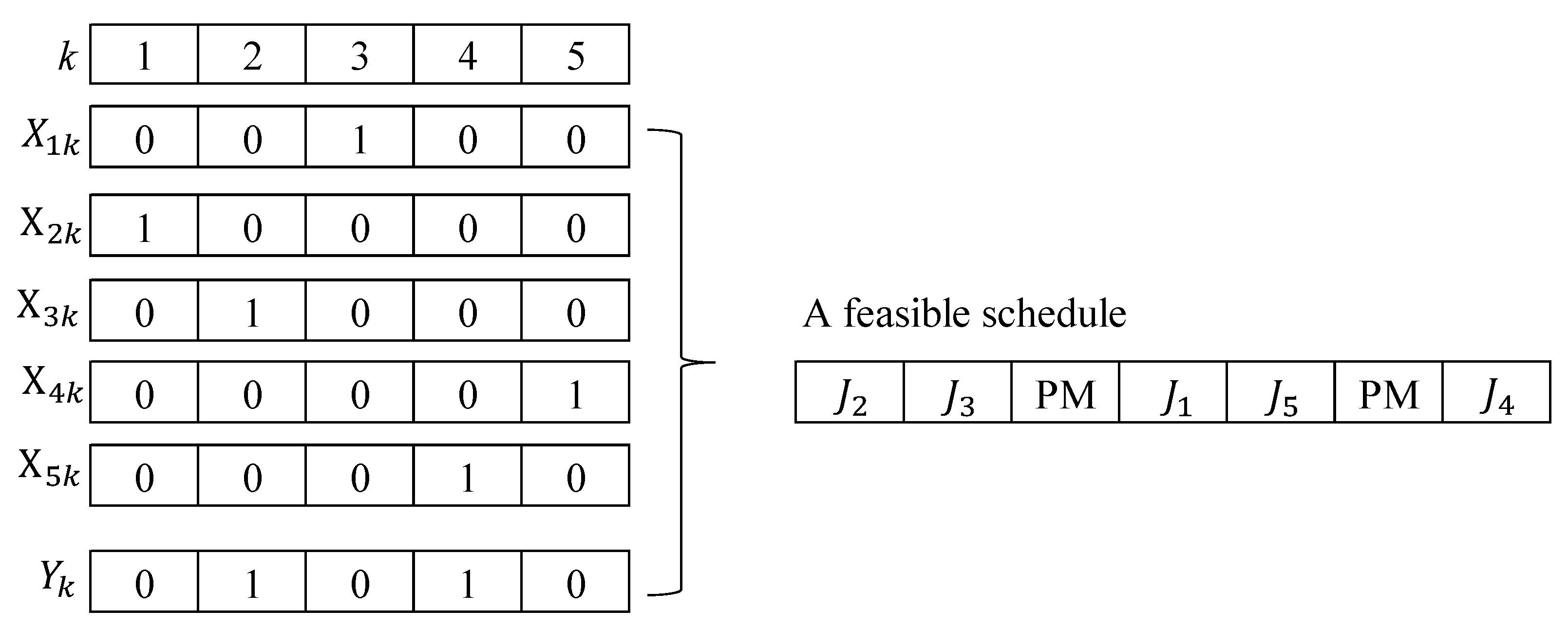
$\mathrm{fitness}\left({\pi }_y\right)=1/\left[TWT\left({\pi }_y\right)+\epsilon \right]$, y = 1, 2,…, population size, where fitness (${\pi }_y$) is the fitness value for the yth chromosome; TWT(${\pi }_y$) is the TWT value; and $\epsilon$ is the smallest value ($\epsilon$ = 0.000001), which aims to keep the denominator greater than zero. To obtain the TWT value for each chromosome, we use the DP method, as mentioned above. In this decoding, the job sequence is based on the relative order in the chromosome, but when to execute PM activities depends on the proposed DP method, as mentioned above. Suppose one of the chromosomes is represented by J₁-J₃-J₄-J₅-J₂ for the 5-job instance shown in Table 2. Using the proposed decoding method, the feasible schedule for the chromosome of J₁-J₃-J₄-J₅-J₂ is obtained, as shown in Figure 3, where the corresponding TWT and fitness values are 41 and 0.0244, respectively.

4.4. Crossover/Mutation

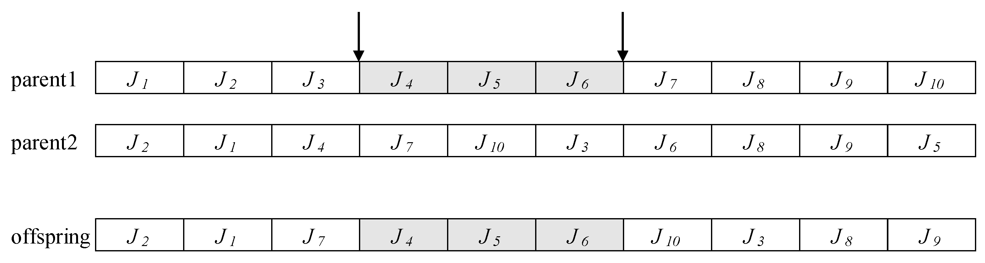
For recombination/crossover to generate offspring, we applied bias roulette wheel selection to choose parents from the pool of the population, which was the first selection operator proposed by Holland in 1975 (Goldberg, 1989). Since then, it has become a common method used in a variety of GA applications. For crossover, we consider order crossover (OX). In the OX crossover, two cutoff points from parent one are randomly selected, and the information between the two cutoff points is added to the generated offspring. The remaining jobs are filled in the order from parent 2. In this way, OX crossover always generates feasible offspring. Figure 4 illustrates an example of an OX crossover.

For each offspring generated by OX crossover, the parent solution’s features may be randomly modified by the mutation operator. The mutation operator preserves a reasonable level of population diversity that helps the GA escape local optima. In this paper, we adopt a swap mutation. More precisely, we produced a random number $r_{mut}$ from uniformly distributed between 0 and 1. If the random number $r_{mut}$ is less than or equal to a given mutation probability $p_{mut}$, i.e., $r_{mut}\le p_{mut}$, then the contents of two random genes of the offspring are swapped.

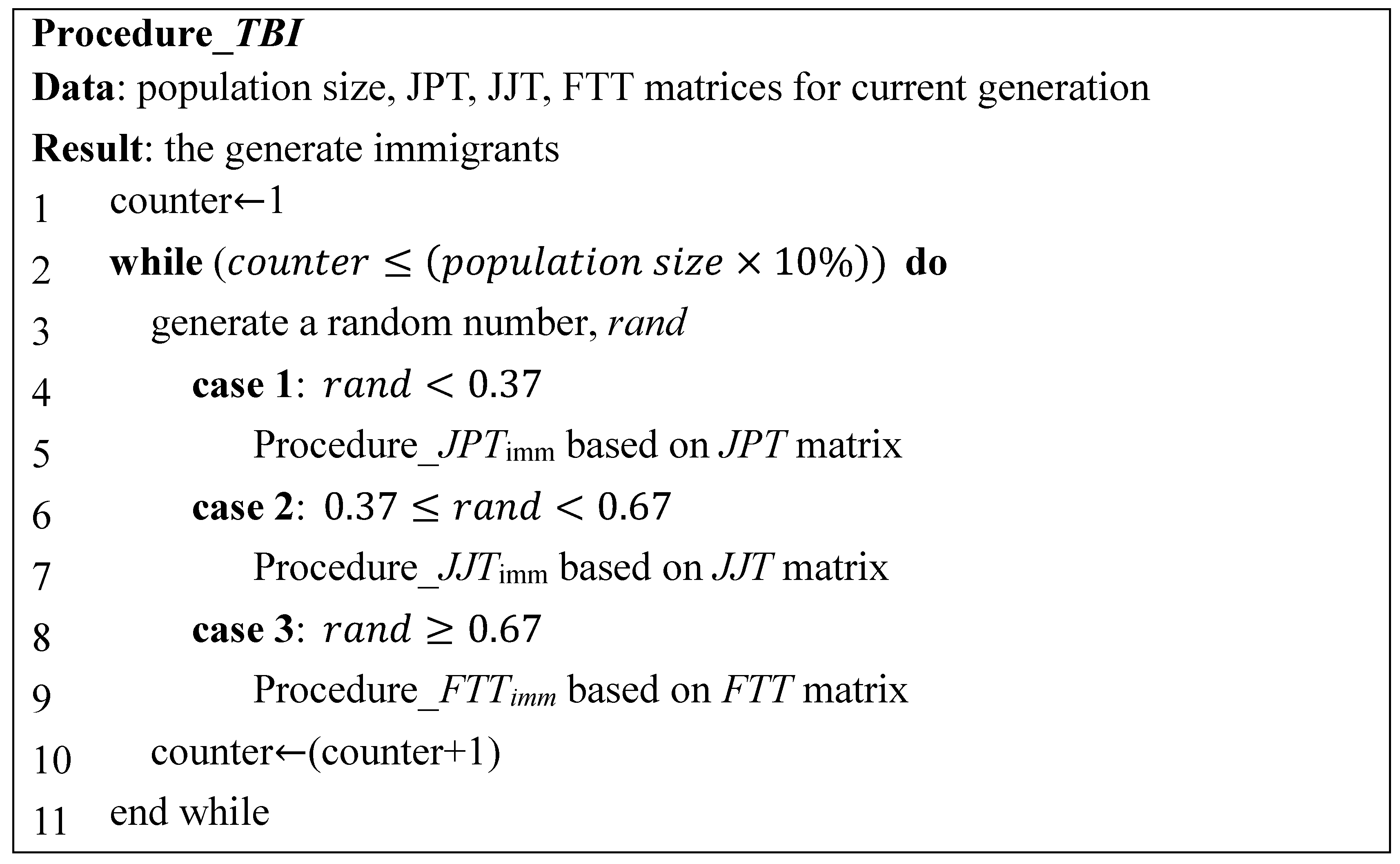
4.5. Immigration

In immigrant schemes, a certain number of immigrants are generated and added to the pool of the population by replacing the worst individuals from the current generation. In this paper, we applied random immigration and trajectory-based immigration strategies addressed in this paper to create immigrants for the next population. For the trajectory-based immigration strategy, the percentage of immigrants generated from JPT, FTT and JJT is 37%, 33% and 30%, respectively, since the first two matrices have a higher correlation with the objective value mentioned above. A bias roulette wheel as the basic selection mechanism is used for producing immigrants based on the information of JPT, JJT and FTT matrices in which a job of higher $v_{jk}$ has a large chance to be selected.

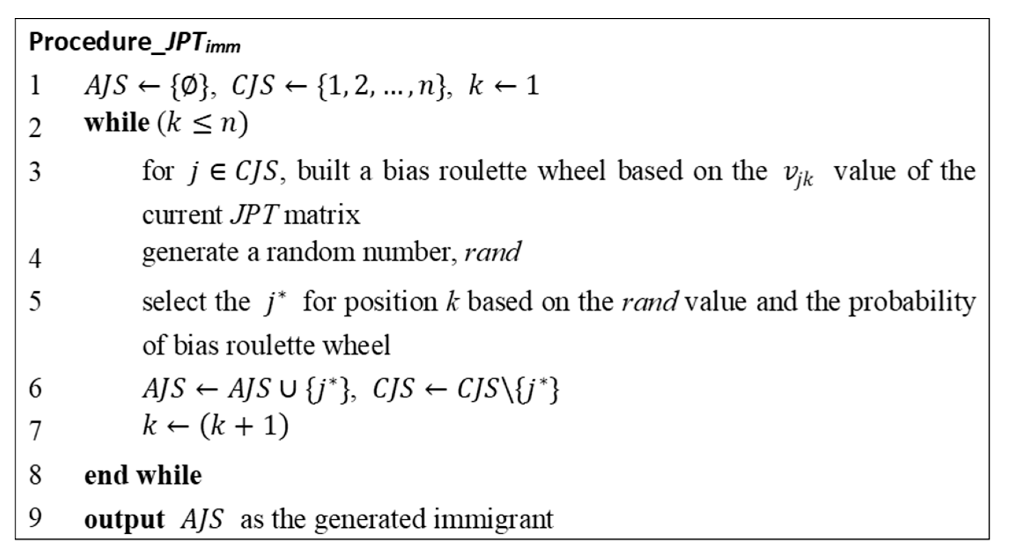
The pseudocode of the trajectory-based immigration procedure and immigrant-creation procedure based on JPT, JJT and FTT are described in Procedure_TBI (seen in Figure 5), Procedure_JPT_imm, Procedure_JJT_imm and Procedure_FTT_imm. Note that the main difference among the three procedures is that the given information to generate immigrants is different, i.e., provided by either JPT, JJT or FTT matrices. Here, we only use Procedure_JPT_imm as an illustration in the following (seen in Figure 6).

It is noted that the value of k in Procedure_$FT{T}_{imm}$ begins from 0, not 1, which is the main difference between Procedure_$FT{T}_{imm}$ and the other two procedures.

4.6. New Generation

For a subsequent generation, first, we used the elitist strategy for reproduction, where 10% of the chromosomes with higher fitness values are automatically copied to the next generation. Second, the worse 10% of chromosomes are directly replaced by new chromosomes generated by “immigration” in the next generation. Finally, 80% of the chromosomes in the next generation come from crossover/mutation. If GA has no immigration scheme, then the rates for reproduction and crossover/mutation are changed to 10% and 90%, respectively.

The pseudocode for the proposed TISGA is described in Figure 7.

5. Computational Experiment

The A comprehensive experiments are conducted; there are 23 test problem sizes n ={5, 6, 7, 8, 9, 10, 15, 20, 25, 30, 35, 40, 45, 50, 60, 70, 80, 90, 100, 200, 300, 400, 500}. Job processing time, release time and weights are generated uniformly on the interval [2, 15], [0, 50] and [1, 10], respectively. The maximum working time limit and maintenance time are L = {15, 30} and MT = 5. Additionally, the due date of each job was generated from a uniform distribution $\left(r_j+p_j\right)+U[(1-\mathrm{TF}-\mathrm{R}/2)\overline{P}, \left(1-\mathrm{TF}+\mathrm{R}/2\right)\overline{P}$], where $\overline{P}$ is the average processing time of all jobs, tardiness factor TF = {0.4, 0.6} and relative range factor of the due date R = {0.4, 0.6}. Ten instances were generated for each of the eight combinations of parameter values (L, TF, R), yielding 80 instances for each value of n. Our MIP model is executed by IBM ILOG CPLEX Optimization Studio Version 12.7.1, and the proposed GA is coded in C++. All tests were conducted on a PC with an Intel Xeon E-2124 3.4 GHz CPU with 32 GB of RAM.

To examine the performance of the proposed TISGA, we also proposed a basic GA without immigration and a GA with a random immigration strategy (GARI). For a fair comparison, all versions of the proposed GAs have $\left(2\times n\right)$ and 100 chromosomes for $\left(n\le 50\right)$ and $\left(n>50\right)$, respectively, and their parameter settings mentioned above are the same. Each version of the GA algorithm is run five times repeatedly to obtain the best result for each instance, and the computational time limit is set to $\left(n\times 0.01\right)$ CPU seconds as the stopping criterion for each version of the GAs.

First, we aim to show the efficiency of the proposed GAs. The proposed MIP model is built to find optimal solutions for small-sized problems since the considered problem here is NP-hard.

Table 8. Comparison of results for MIP and GAs for small-sized problems.

n	Combinations (L, TF, R)	AveTWT				Nopt
		MIP	Basic GA	GARI	TISGA	MIP	Basic	GARI	TISAB
5	(1,1,1)	75.700	75.700	75.700	75.700	10	10	10	10
	(1,1,2)	108.900	108.900	108.900	108.900	10	10	10	10
	(1,2,1)	217.000	217.000	217.000	217.000	10	10	10	10
	(1,2,2)	203.200	203.200	203.200	203.200	10	10	10	10
	(2,1,1)	35.700	35.700	35.700	35.700	10	10	10	10
	(2,1,2)	50.900	50.900	50.900	50.900	10	10	10	10
	(2,2,1)	127.800	127.800	127.800	127.800	10	10	10	10
	(2,2,2)	132.900	132.900	132.900	132.900	10	10	10	10
6	(1,1,1)	178.300	178.300	178.300	178.300	10	10	10	10
	(1,1,2)	119.200	119.200	119.200	119.200	10	10	10	10
	(1,2,1)	229.800	229.800	229.800	229.800	10	10	10	10
	(1,2,2)	207.300	207.300	207.300	207.300	10	10	10	10
	(2,1,1)	62.600	62.600	62.600	62.600	10	10	10	10
	(2,1,2)	94.500	94.500	94.500	94.500	10	10	10	10
	(2,2,1)	190.000	190.000	190.000	190.000	10	10	10	10
	(2,2,2)	226.900	226.900	226.900	226.900	10	10	10	10
7	(1,1,1)	283.200	283.200	283.200	283.200	10	10	10	10
	(1,1,2)	227.700	227.700	227.700	227.700	10	10	10	10
	(1,2,1)	340.900	340.900	340.900	340.900	10	10	10	10
	(1,2,2)	321.700	324.700	324.700	324.700	10	9	9	9
	(2,1,1)	101.100	101.100	101.100	101.100	10	10	10	10
	(2,1,2)	173.900	173.900	173.900	173.900	10	10	10	10
	(2,2,1)	185.800	185.800	185.800	185.800	10	10	10	10
	(2,2,2)	245.300	245.300	245.300	245.300	10	10	10	10
8	(1,1,1)	343.200	343.200	343.200	343.200	10	10	10	10
	(1,1,2)	252.300	252.600	252.600	252.600	10	9	9	9
	(1,2,1)	556.300	556.300	556.300	556.300	10	10	10	10
	(1,2,2)	337.900	337.900	337.900	337.900	10	10	10	10
	(2,1,1)	134.700	134.700	134.700	134.700	10	10	10	10
	(2,1,2)	181.000	181.000	181.000	181.000	10	10	10	10
	(2,2,1)	224.300	224.300	224.300	224.300	10	10	10	10
	(2,2,2)	356.400	356.400	356.400	356.400	10	10	10	10
9	(1,1,1)	336.700	336.700	336.700	336.700	10	10	10	10
	(1,1,2)	461.200	461.200	461.200	461.200	10	10	10	10
	(1,2,1)	595.500	595.500	595.500	595.500	10	10	10	10
	(1,2,2)	477.100	478.400	478.400	478.400	10	8	8	8
	(2,1,1)	331.200	331.200	331.200	331.200	10	10	10	10
	(2,1,2)	148.100	148.100	148.100	148.100	10	10	10	10
	(2,2,1)	357.000	357.000	357.000	357.000	10	10	10	10
	(2,2,2)	463.500	463.500	463.500	463.500	10	10	10	10
10	(1,1,1)	432.100	432.100	432.100	432.100	10	10	10	10
	(1,1,2)	565.500	565.500	565.500	565.500	10	10	10	10
	(1,2,1)	612.500	612.500	612.500	612.500	10	10	10	10
	(1,2,2)	659.900	667.900	667.900	667.900	10	9	9	9
	(2,1,1)	421.000	421.000	421.000	421.000	10	10	10	10
	(2,1,2)	475.000	475.000	475.000	475.000	10	10	10	10
	(2,2,1)	328.900	328.900	328.900	328.900	10	10	10	10
	(2,2,2)	525.500	525.500	525.500	525.500	10	10	10	10
15	(1,1,1)	1158.800	1158.800	1158.800	1158.800	8	8	8	8
	(1,1,2)	1284.500	1293.300	1284.500	1284.500	8	7	8	8
	(1,2,1)	1982.300	1982.300	1982.300	1982.300	5	5	5	5
	(1,2,2)	1613.700	1612.000	1612.000	1612.000	6	6	6	6
	(2,1,1)	1210.600	1210.600	1210.600	1210.600	7	7	7	7
	(2,1,2)	1038.100	1038.100	1038.100	1038.100	10	10	10	10
	(2,2,1)	1284.300	1284.300	1284.300	1284.300	7	7	7	7
	(2,2,2)	1079.500	1079.500	1079.500	1079.500	10	10	10	10

shows the average TWT values (AveTWT) and the number of optimal solutions found by each algorithm for small-sized problems. The results obtained by the GA algorithms that are worse (higher) than those obtained by the MIP model are presented in boldface. From Table 8, even with a small increment of n (n = 15), it becomes impossible for the MIP model to reach optimal solutions within a reasonable computational time, where the computational time limit for the MIP model is set to 7200 s. Additionally, the three versions of the proposed GAs are almost equivalent when comparing the average TWT value and Nopt. Regarding the average computational time shown in

Table 9. The average computational time required by the MIP model and GAs.

n	MIP	All Versions of GAs
5	0.050	0.050
6	0.061	0.059
7	0.083	0.070
8	0.212	0.079
9	0.536	0.090
10	1.663	0.100
15	2854.086	0.150

Remark: For n = 15, there are 19 instances in which computational time solved by the MIP model exceeds 7200 s.

, note that the computational time limit of all versions of the GAs is the same as $\left(n\times 0.01\right)$ seconds. This experiment demonstrates that the MIP model is very expensive regarding the computational cost when n = 15. On the other hand, the GA performances are very reliable in finding the optimal solutions in less than 0.15 s. Therefore, this experiment justified that the development of GAs can reduce the computational effort without seriously losing solution quality.

Recall that the MIP model cannot find all optimal solutions within 7200 s, and the basic GA becomes slightly worse on solution quality when n = 15. Thus, we further investigate the performances of different GAs for large-sized problems in the second experiment. Please note that the computational time limits of the GAs are the same, i.e., $\left(n\times 0.01\right)$ seconds, for each n. For comparison, we apply the relative percentage deviation (RPD) of each instance computed as follows.

$\mathrm{RPD}=\left[\left(TWT\left(A\right)-Min\right)/Min\right]\times 100\%$, where Min is the lowest TWT value for a given instance obtained by any of the GA algorithms, and TWT(A) is the TWT value obtained for a given algorithm and instance. AveRPD refers to Average RPD.

Table 10. Comparison of results for GAs for large-sized problems.

	AveRPD			Nbest
n	Basic GA	GARI	TISGA	Basic GA	GARI	TISGA
20	0.126	0.180	0.000	68	64	80
25	0.545	0.369	0.015	40	48	79
30	0.731	0.490	0.005	19	22	79
35	1.121	0.834	0.000	4	6	80
40	1.012	0.908	0.001	2	8	78
45	0.997	0.994	0.000	1	1	80
50	1.409	1.325	0.005	2	1	79
60	1.209	1.317	0.000	0	0	80
70	1.440	1.271	0.001	0	1	79
80	1.384	1.188	0.000	0	0	80
90	1.733	1.349	0.000	0	0	80
100	2.045	1.419	0.000	0	0	80
200	4.572	3.315	0.000	0	0	80
300	6.110	4.896	0.000	0	0	80
400	7.074	6.055	0.000	0	0	80
500	5.944	5.083	0.028	0	5	75
mean	2.341	1.937	0.003	8.50	9.75	79.31

shows the AveRPD and the total number of best solutions (Nbest) obtained by each GA. As depicted in the table, GARI finds slightly better solutions than the basic GA; that is, 1.937% is obtained by GARI, while the basic GA gives a mean AveRPD value of 2.341%. Overall, TISGA significantly outperforms GARI and basic GA because the total number of best solutions obtained by the proposed TISGA is 1269, 136 for basic GA, and 156 for GARI among 1280 instances. The results support our inference that GAs maintain the diversity level of the population through immigration strategy to achieve a better quality of solutions. Furthermore, the proposed trajectory-based immigration strategy enhances the effectiveness of the GA method more than the random immigration strategy.

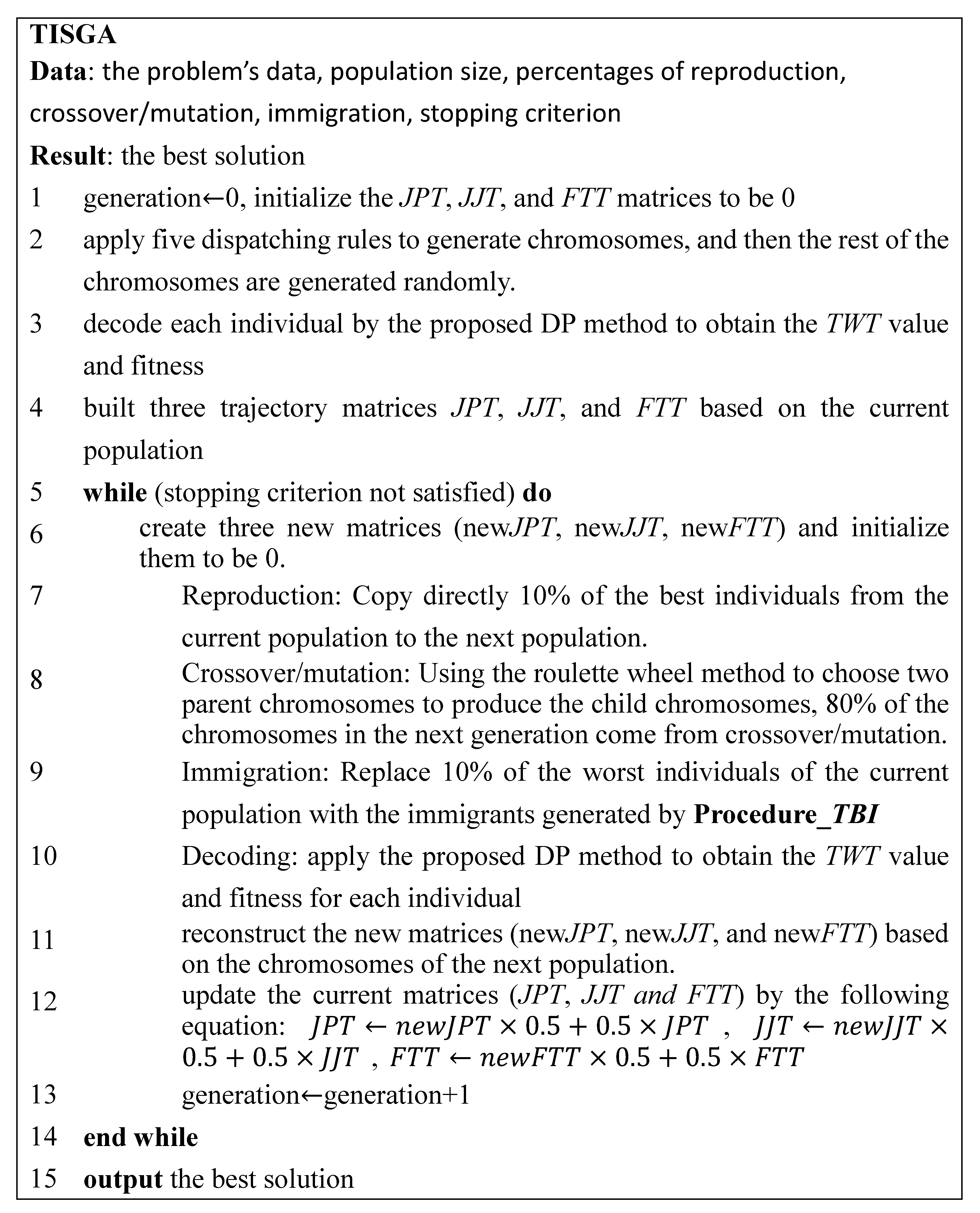
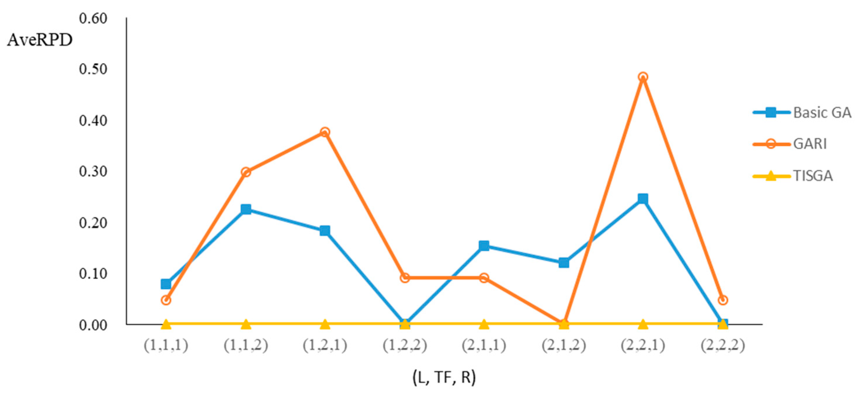
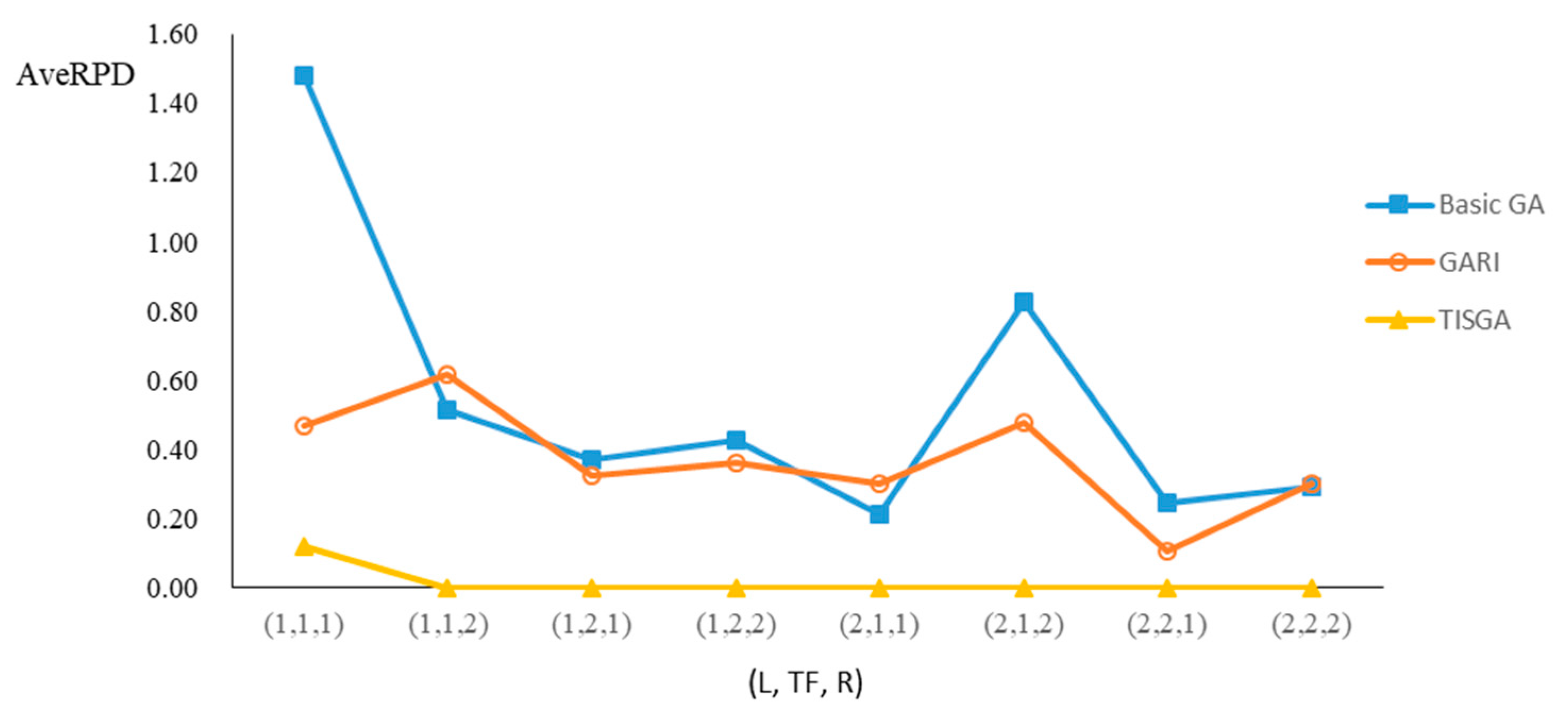
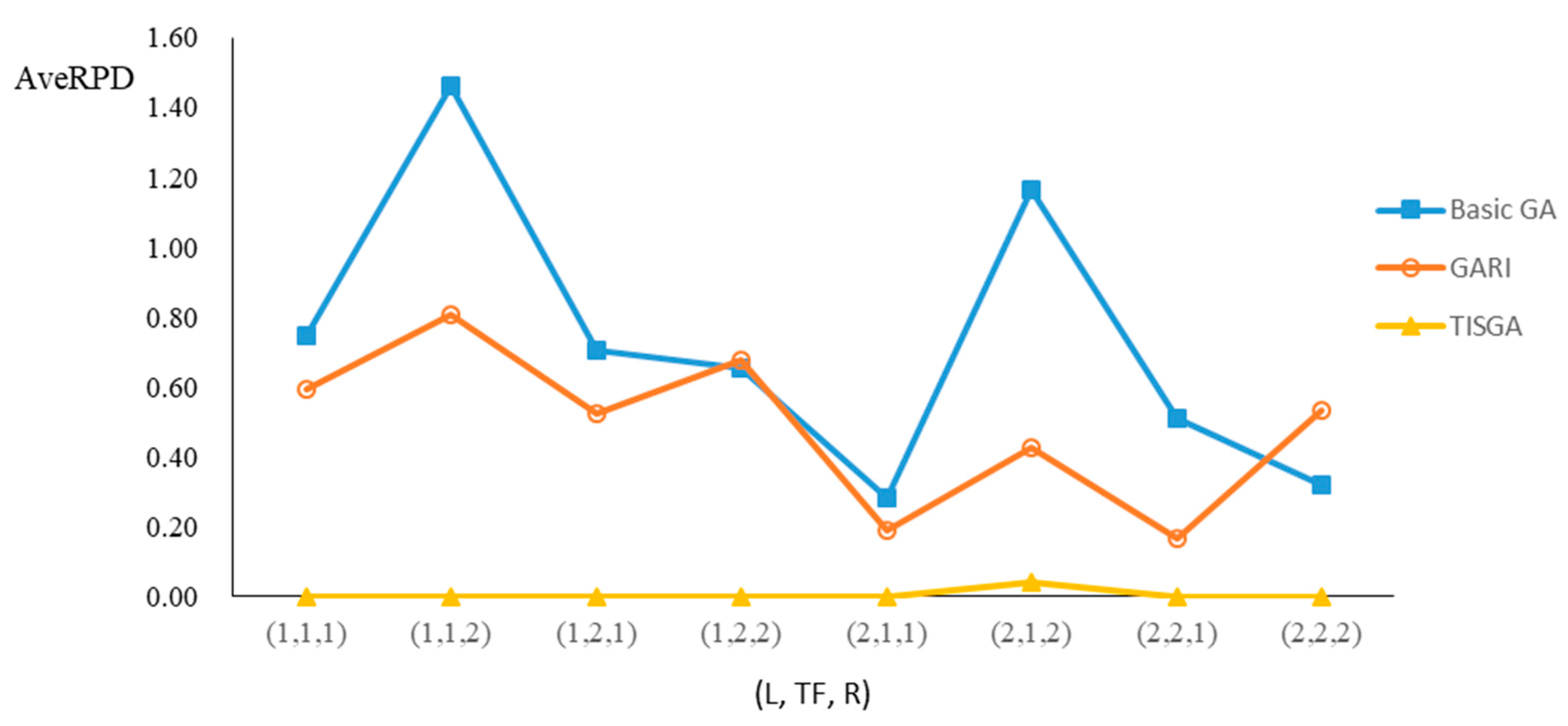
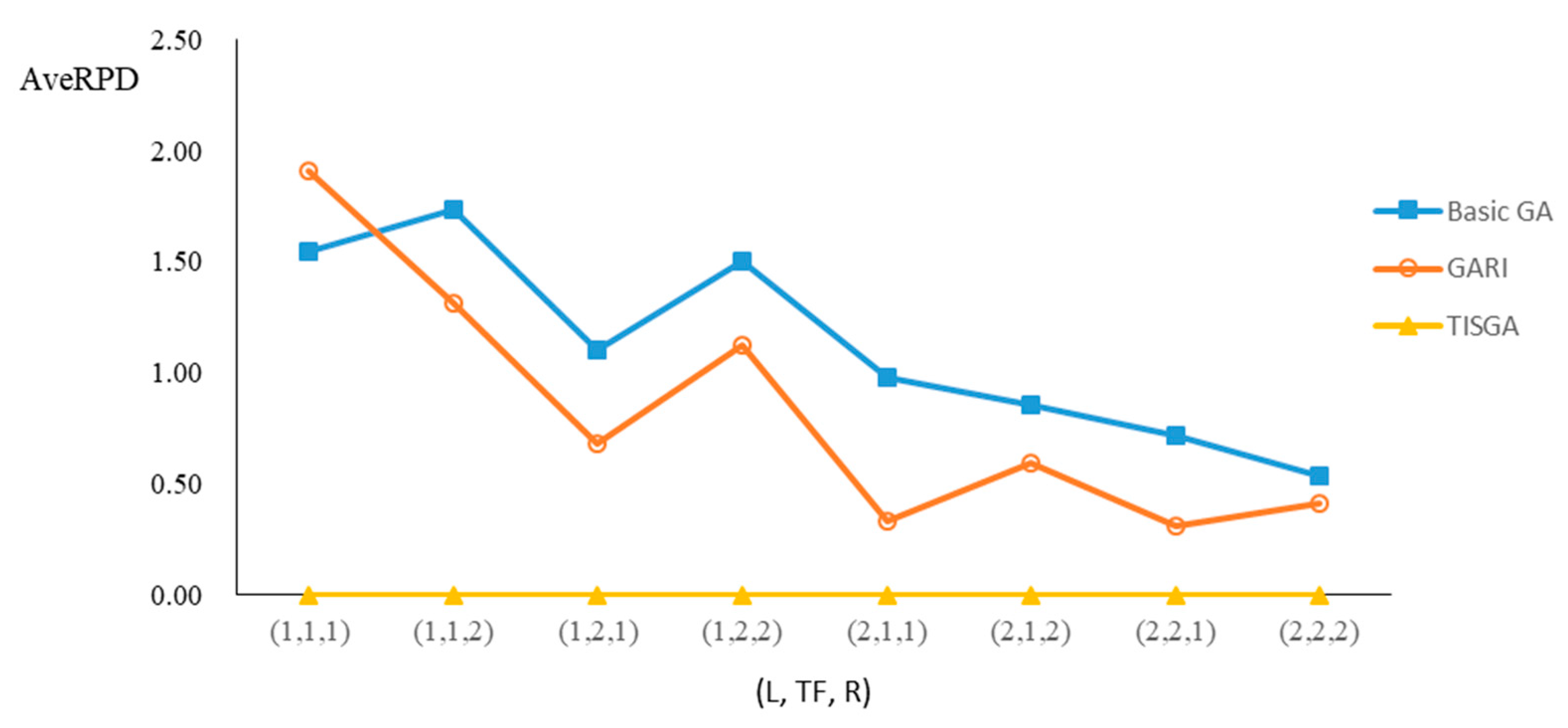
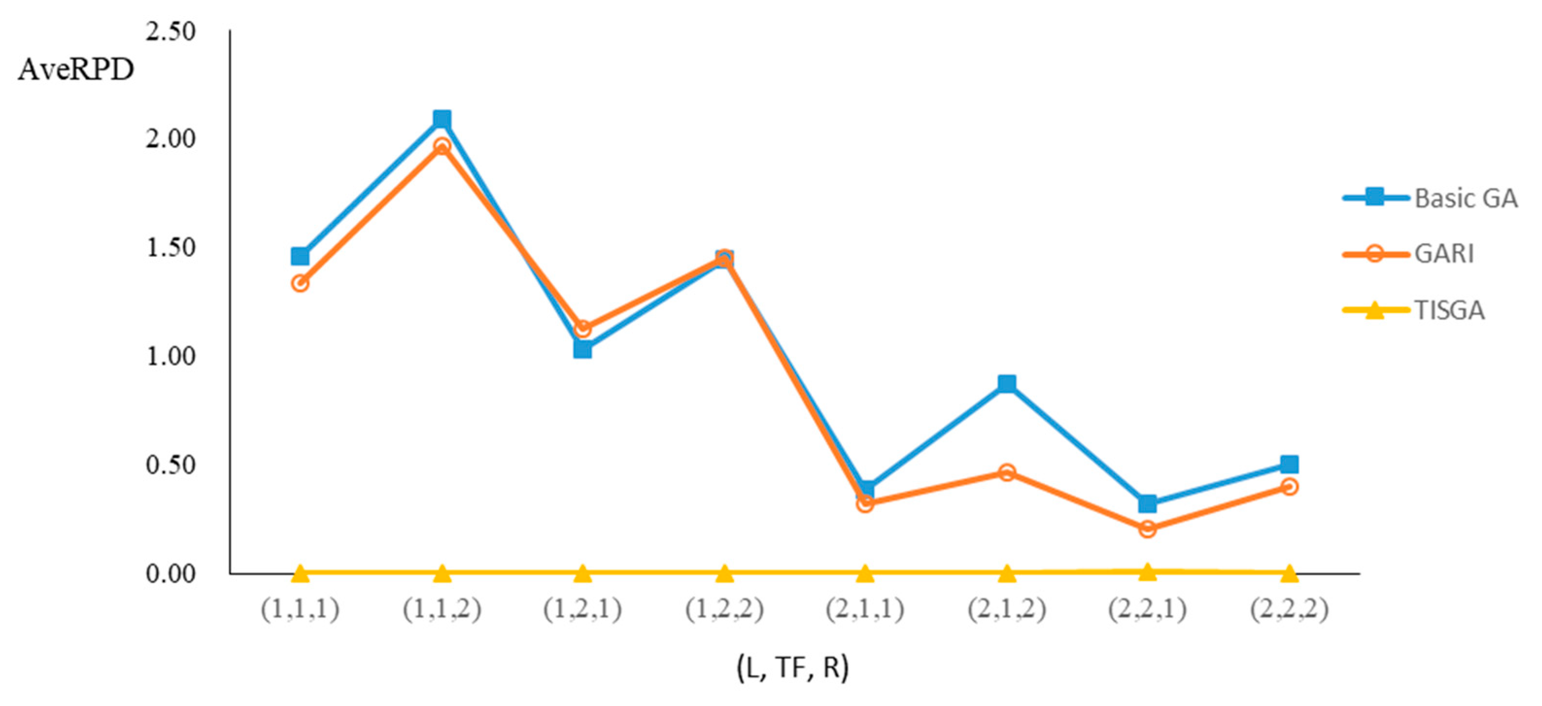
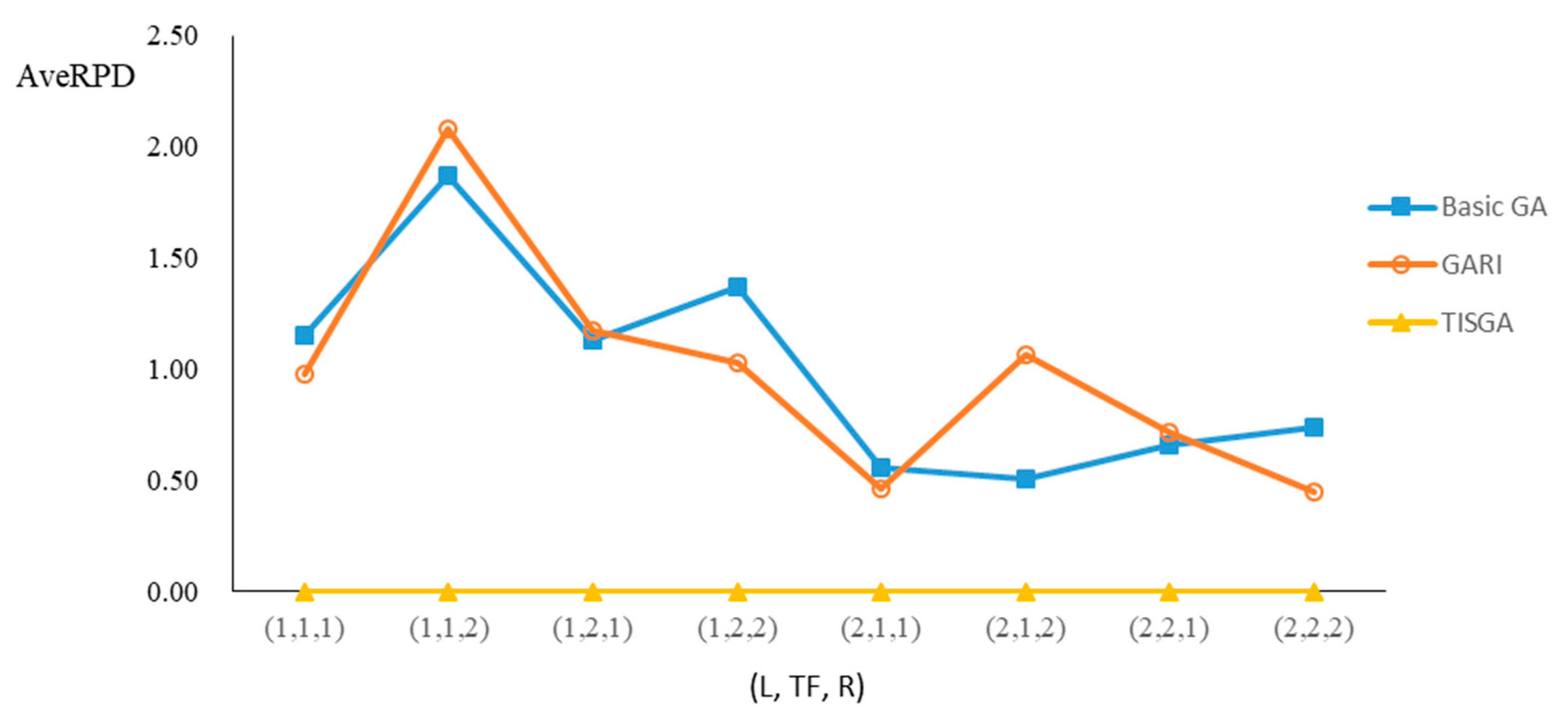
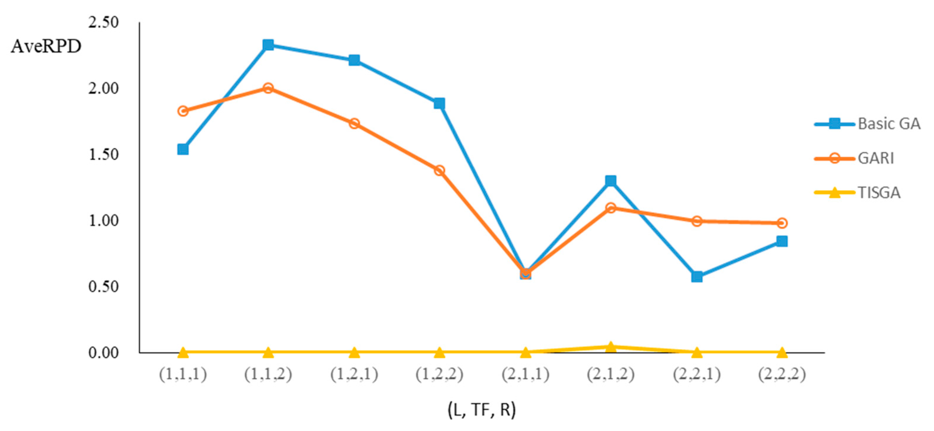
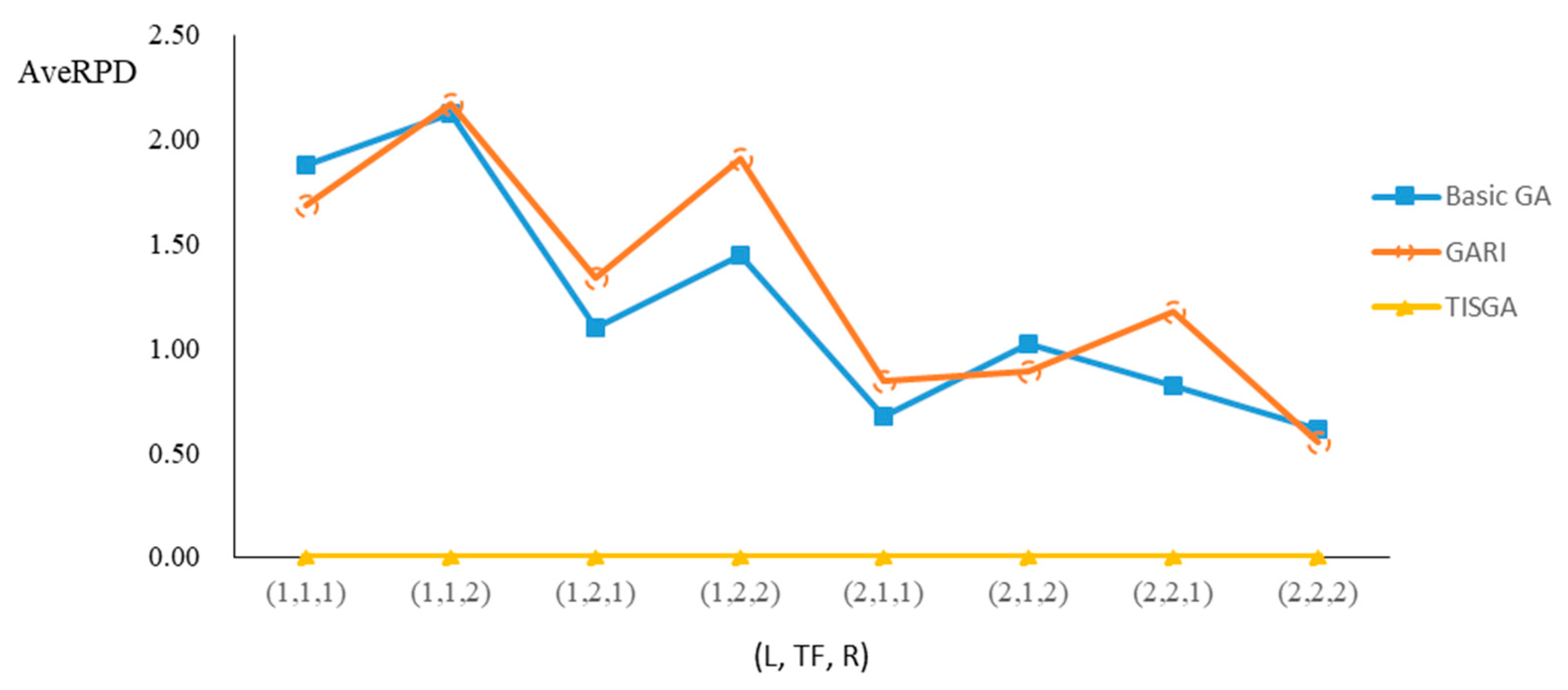
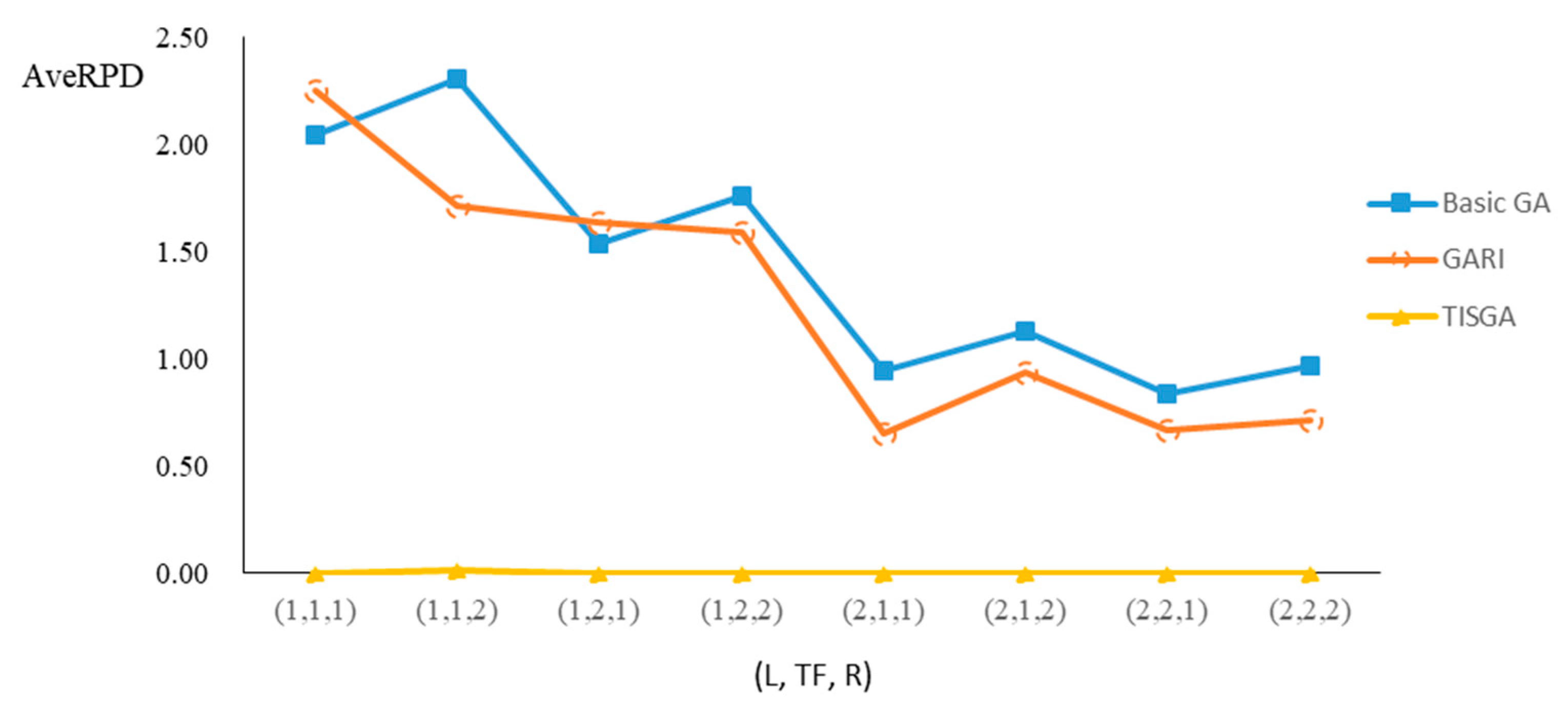
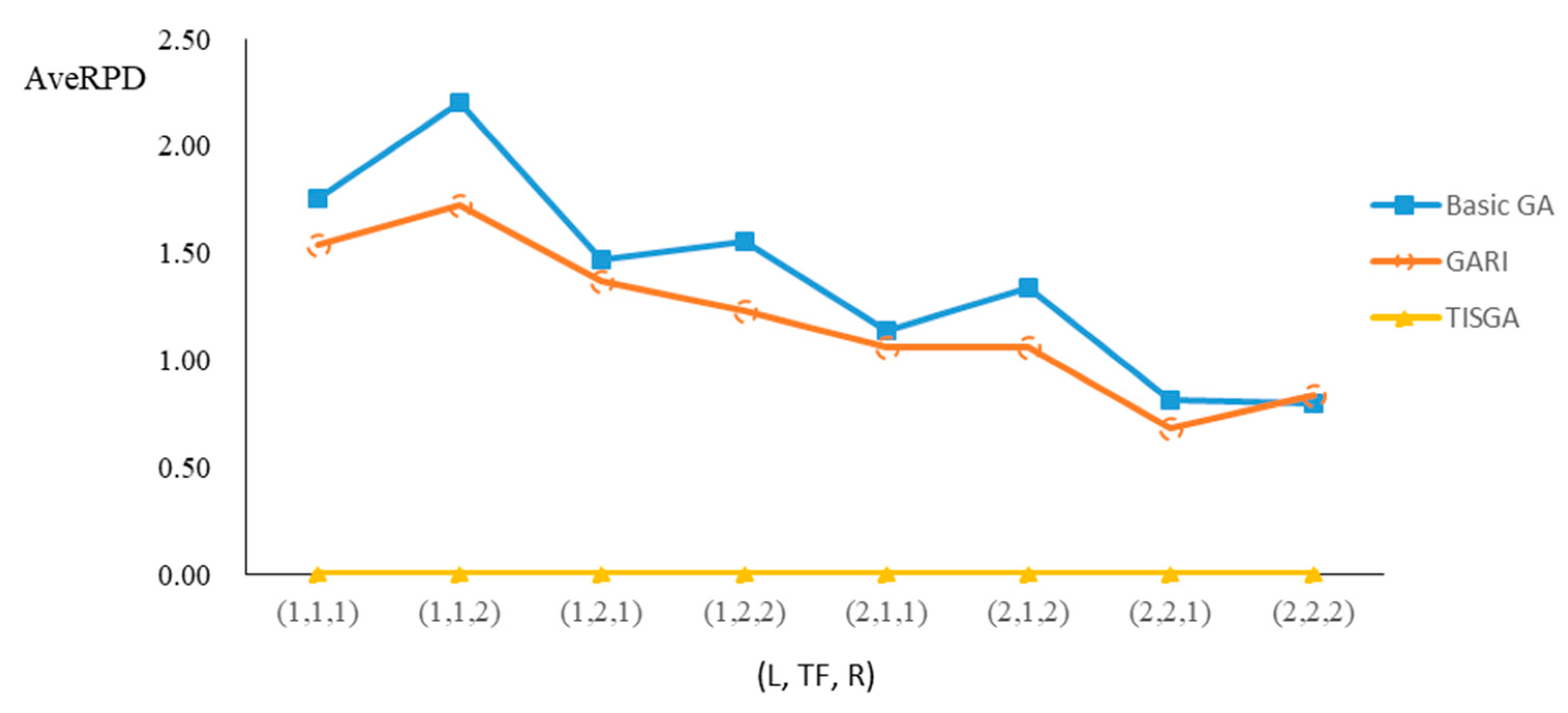
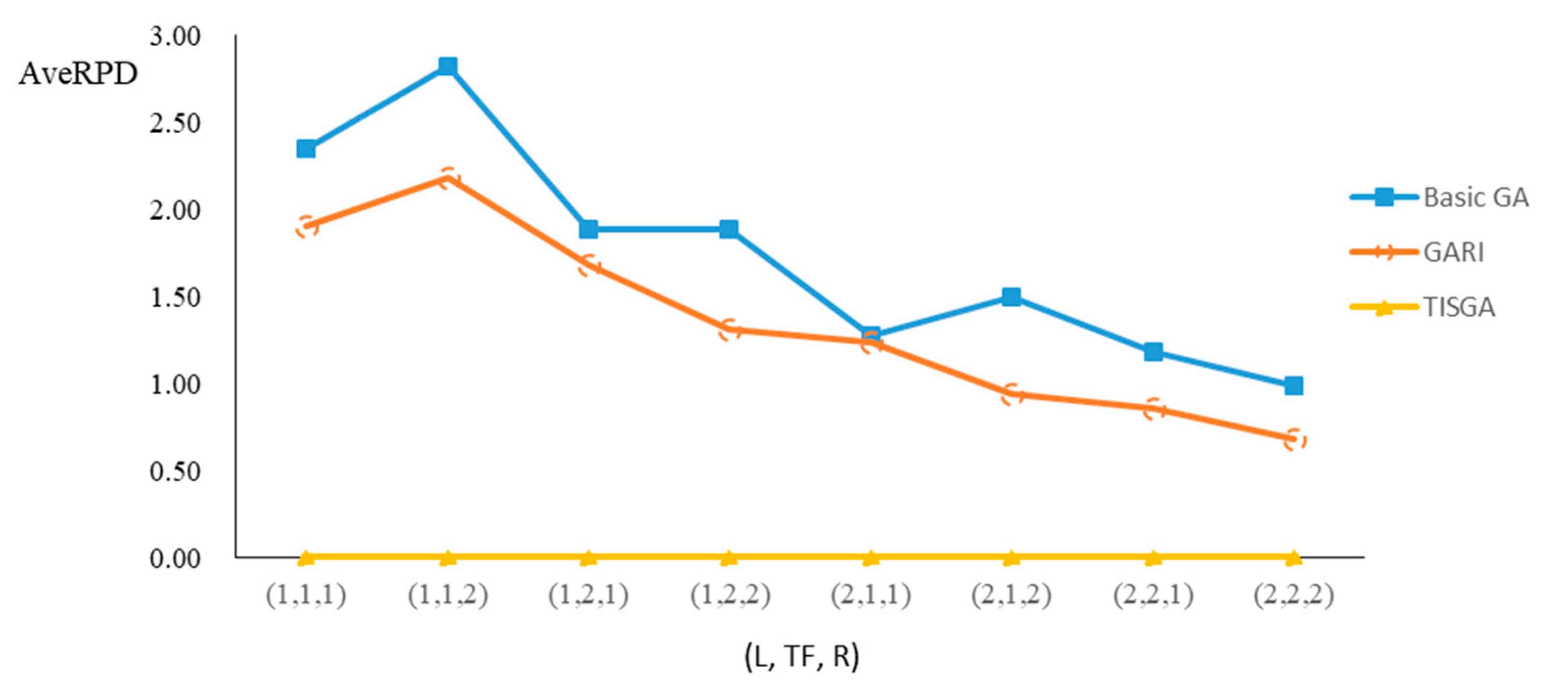
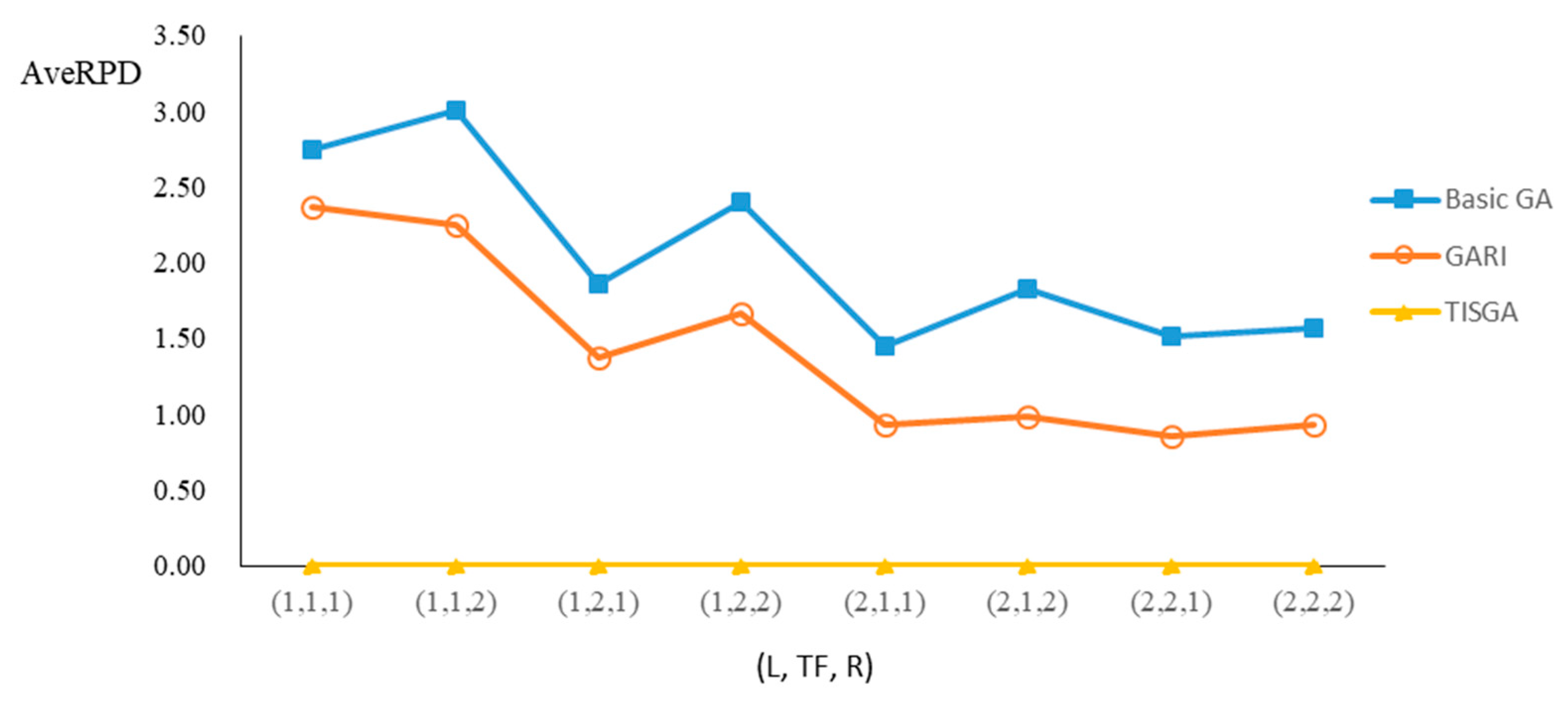
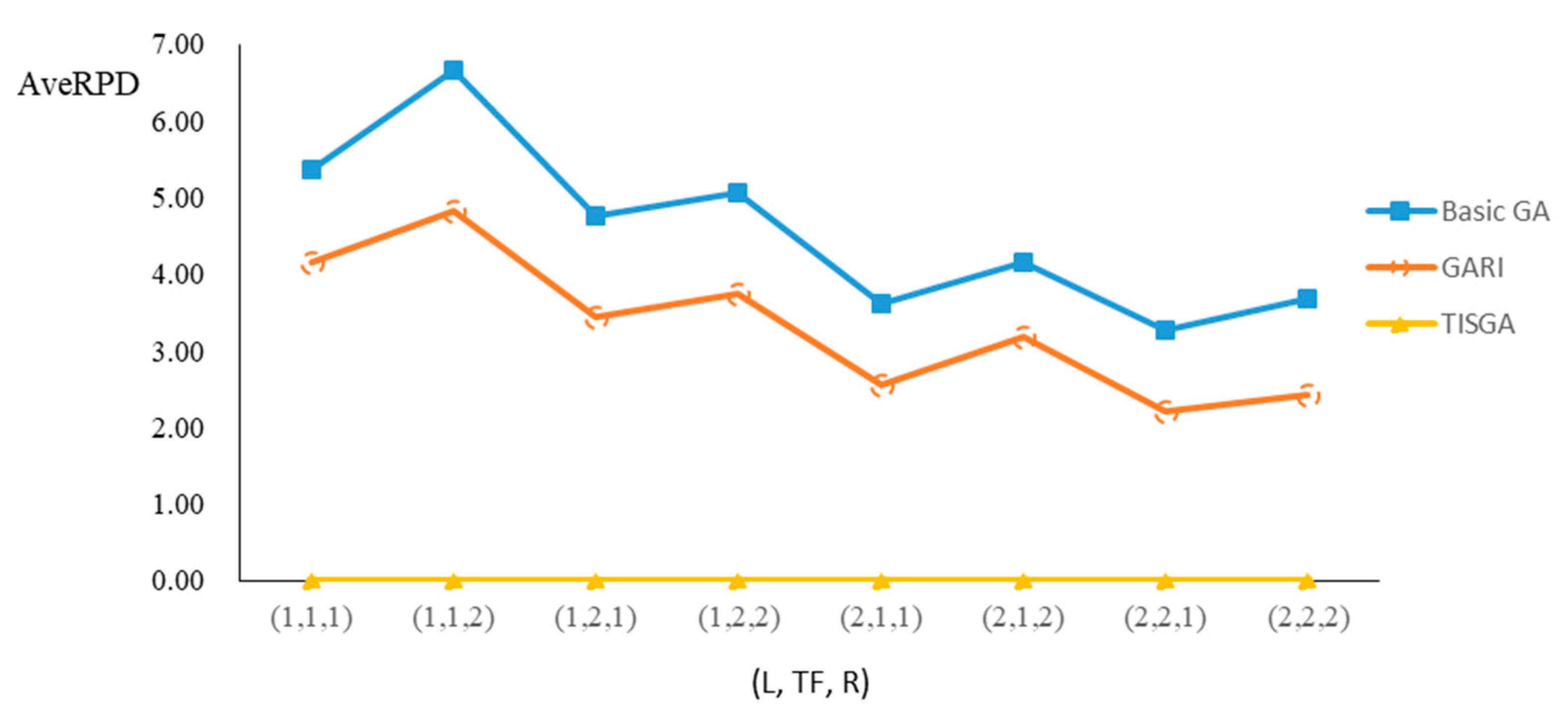
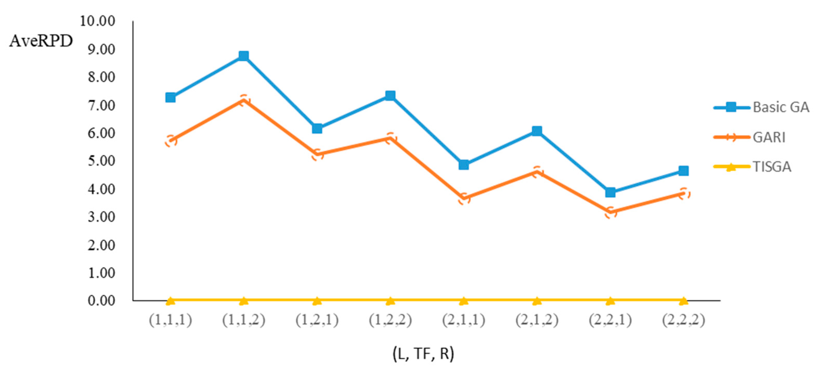
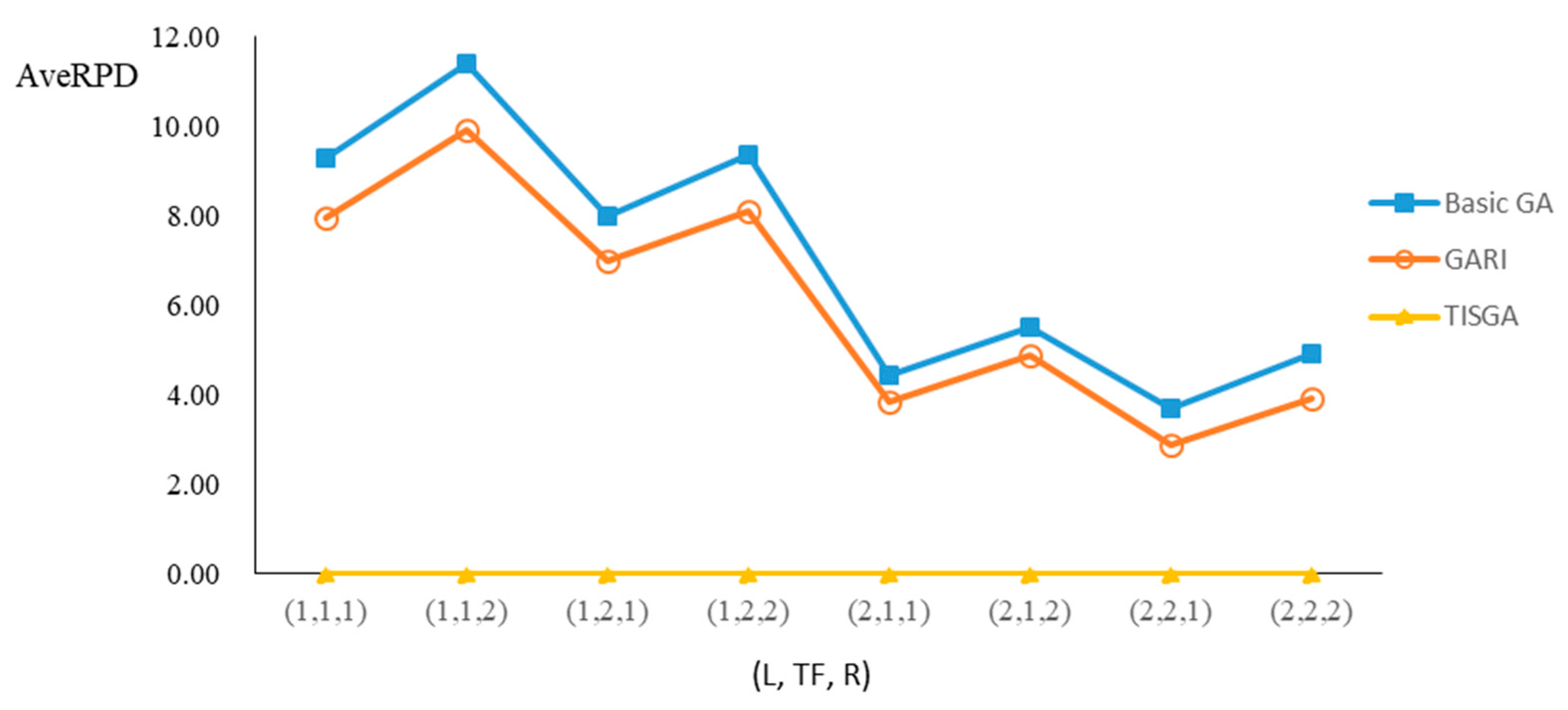
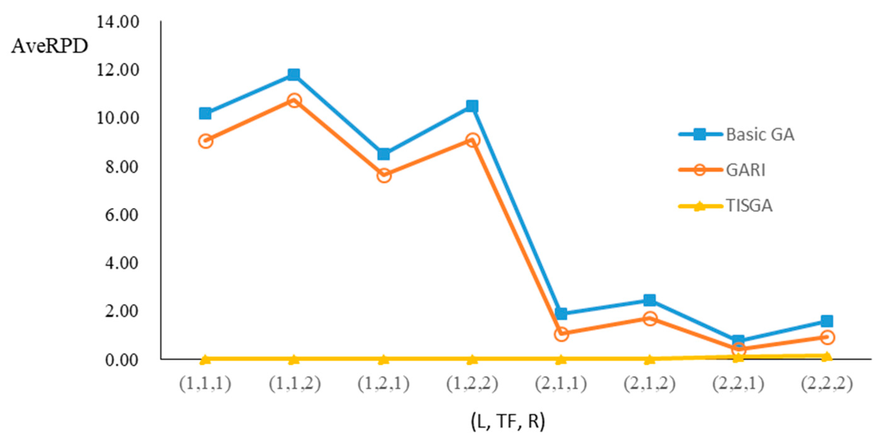
We also examined the performance of GAs under different combinations of (L, TF, R) for each problem. Figure 8, Figure 9, Figure 10, Figure 11, Figure 12, Figure 13, Figure 14, Figure 15, Figure 16, Figure 17, Figure 18, Figure 19, Figure 20, Figure 21, Figure 22 and Figure 23 illustrate the comparison results under eight combinations of (L, TF, R) for large-sized problems. From these figures, in some cases, GARI is worse than the basic GA; that is, the performances of GARI and the basic GA are influenced by the values of (L, TF, R). However, as the number of jobs increases, GARI becomes gradually better than the basic GA for any combination of (L, TF, R) because adding randomly generated immigrants helps increase the diversity of solutions for the GA method, especially for larger job sizes. The proposed TISGA overcomes the influence of combinations of (L, TF, R) on solutions and is robust in obtaining better solutions.

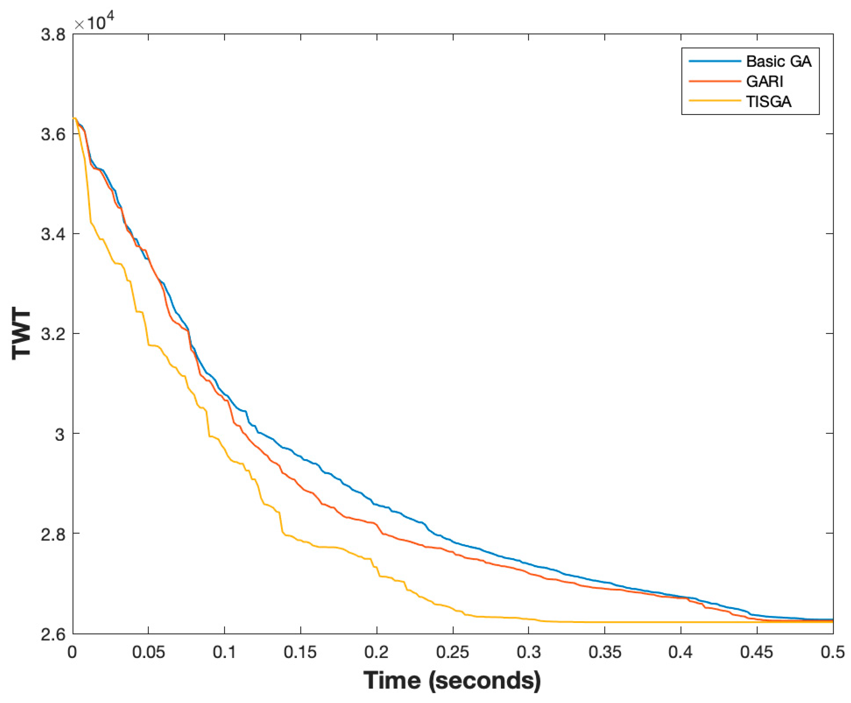
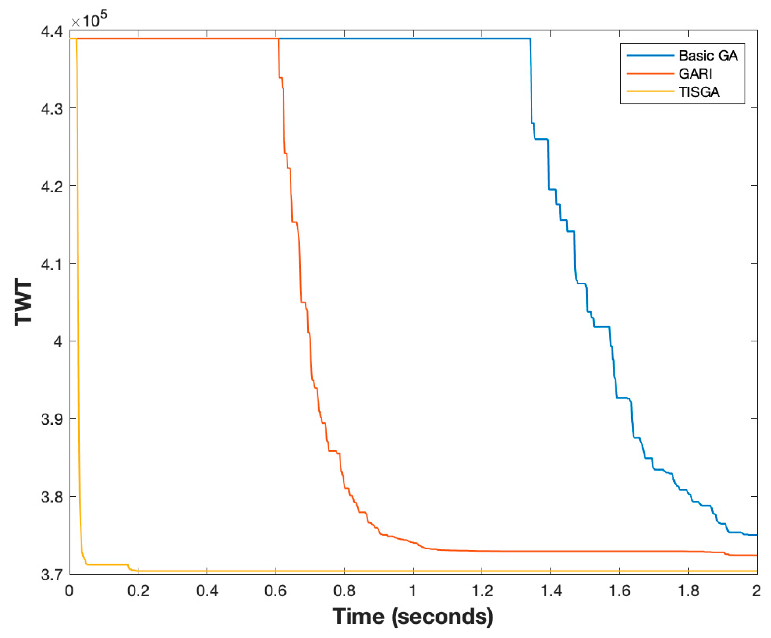
Better convergence is another important topic for designing a good GA method. Thus, we compared the convergence of the basic GA, GARI and TISGA using instances with n = 50 and n = 200, respectively, as shown in Figure 21 and Figure 22. From Figure 24 and Figure 25, the convergence speed in TISGA is highest among GARI and the basic GA, and the solutions obtained by TISGA require less computation time than those required by GARI and the basic GA. Through these experimental results, we conclude that coupling a GA with the trajectory-based immigration scheme accelerates the convergence speed and significantly improves the performance of the basic GA.

6. Discussions

Based on the comparison results in Section 5, we use nonparametric tests under α = 0.05 confidence level to examine the superiority of the proposed TISGA; it was verified that, when the size of the problem is small, the immigrant strategy does not induce significantly the quality of the final solution, since the hypothesis Basic GA = GARI and GARI = TISGA cannot be rejected with significance 0.317 and 1.000, respectively. It is reasonable that, when the problem is small, solution space can almost be searched by basic GA without adding any improved scheme. For large-size problems, the hypothesis Basic GA = GARI and GARI = TISGA are rejected with the significance of 0.002 and 0.000, respectively, which showed that the proposed immigrant strategy induces significantly the solution quality of GA.

Overall, the proposal TISGA has the following features and advantages when compared with GAs:

• With the problem being NP-hard, it is tough to search for all solutions when the size of the problem increases. In this case, a good search scheme, such as the proposed trajectory-based immigration strategy to direct GA to obtain a better or optimal solution, is important.
• The possibility to converge to solutions with good quality more quickly due to the trajectory-based immigration strategy.

7. Conclusions

In this paper, we have addressed the single-machine scheduling problem with job release time and flexible preventive maintenance to minimize TWT. To the best of our knowledge, this problem with the TWT objective has not yet been addressed in the literature. For this problem, some JPT, JJT and FTT matrices are established based on the concept of the experience-driven knowledge scheme. Equipped with these matrices, we proposed a GA coupled with a trajectory-based immigration strategy, called TISGA, to generate immigrants to maintain the population diversity of a GA.

To examine the performance of TISGA, we formulated a MIP model and two GAs; one is the basic GA without an immigration strategy, and the other is GARI with a randomly generated immigration strategy. For small-sized problems, GARI and TISGA exhibited the same performances in terms of AveTWT and Nopt as compared to the MIP model. For large-sized problems, 1269 of the 1280 (99.14%) best solutions were found by TISGA, and then 12.18% and 10.63% were obtained by GARI and the basic GA, respectively. The results showed that TISGA outperformed the GARI and basic GA methods. Furthermore, our TISGA showed robust performance with respect to different values of (L, TF, R). More specifically, the results have shown that embedding the proposed trajectory-based immigration strategy in a GA has been enough to obtain excellent solutions for the problem under consideration. Consequently, further research could come in developing more efficient and advanced metaheuristics, successfully adapting the concept of an experience-driven knowledge scheme. Additionally, other potential extensions of this study, including parallel machines, job shops and sequence-dependent setup times, can be made for future research.