Detection of Plausibility and Error Reasons in Finite Element Simulations with Deep Learning Networks

Abstract

The field of application of data-driven product development is diverse and ranges from requirements through the early phases to the detailed design of the product. The goal is to consistently analyze data to support and improve individual steps in the development process. In the context of this work, the focus is on the design and detailing phase, represented by the virtual testing of products through Finite Element (FE) simulations. However, due to the heterogeneous data of a simulation model, automatic use is a big challenge. A method is therefore presented that utilizes the entire stock of calculated simulations to predict the plausibility of new simulations. Correspondingly, a large amount of data is utilized to support less experienced users of FE software in the application. Thus, obvious errors in the simulation should be detected immediately with this procedure and unnecessary iterations are therefore avoided. Previous solutions were only able to perform a general plausibility classification, whereas the approach presented in this paper is intended to predict specific error sources in FE simulations.

1. Introduction

The systematic analysis of data is increasingly established in the product development process and referred to as data-driven product development [1,2,3]. The range of application is broad, starting at the requirements and continuing through the early phases to the detailed specification of the product. The fundamental principle is the consistent analysis of data to support and improve dedicated (sub-)steps. According to [1], the procedure can be divided into dataset, knowledge base, data-driven method, and the design process step. For each stage, the possibilities are highly dependent on the associated constraints.

In the context of this paper, the focus is on the design and detailing phase, especially on the virtual testing of the products with Finite Element simulations. Due to the heterogeneous data in a simulation model, consisting of input (3D geometry, load cases, surface meshes, etc.), model (mesh, solving methods), and output data (results, reports, etc.), the automatic use of this data is a major challenge [4,5]. An approach for reusing FE simulations was developed by [6], which allows for the retrieval of specific simulations via a database system. As a result, only certain simulations are reused, not the entire pool of calculated simulations. The large amount of data is normally only kept for legal purposes but should be utilized to enable a system to predict the plausibility of new simulations. The aim is to support less experienced users of FE software in their application by directly identifying obvious errors in the simulation and thus avoiding unnecessary iterations. While previous solutions were only able to make general plausibility classifications, the approach presented here targets the prediction of specific error sources. The challenge is to define a suitable transformation method for the simulation data and train a model that is able to predict error sources with high accuracy.

1.1. State of the Art

The intention to support users in the application of FE software has been present in the academic landscape for a long time. A very early knowledge-based system was presented by [7] in the late 1980s. With the help of the SACON (Structural Analysis CONsultant) system, the FE calculation of Boeing 747 wings could be improved and access for less experienced engineers was facilitated. Another analysis tool that enhances FE simulation with knowledge-based engineering (KBE) was introduced by [8], with the aim of supporting set up of the FE simulation through knowledge databases. The system was demonstrated with aluminum draw bending components as an example.

In addition to knowledge-based approaches, the use of Machine Learning (ML) techniques in combination with FE simulations has also become popular for facilitating FE simulation tasks. To improve material generation, an approach was presented by [9] that assists the modeling of materials through evolutionary polynomial regression. The approach was integrated into the existing FE simulation process and tested for linear elastic and elastic–plastic material models. The preparation of geometry, a sub-step of preprocessing, can also be optimized by Machine Learning methods. For example, [10] developed a method that detects different ribbon features in components, which enables high-quality meshing of these geometric features. In addition to the recognition, a decomposition into individual areas is also essential for generating a suitable mesh. Another preprocessing upgrade was created from [11], which describes hole detection for mold injection parts. The identified holes are removed from the parts in a subsequent step to facilitate and accelerate the meshing of the different mold components. Furthermore, a contribution dealing with the automatic geometric simplification of components was created by [12]. This approach relies on geometric primitives for segmentation and following morphological investigations of the component. The methods generate a simplified surface model for the simulation from the 3D volume model through dimensional reduction and fitting of the contact surfaces. The authors of [13] provided another contribution to the automation of the preprocessing process by building ontologies via text and data mining, which builds the foundation of the simulation model. In this context, standards or simulation reports serve as the source of the knowledge base and help to automatically set up the simulation. Depending on the analysis requirement, the simulation can be set up accordingly, such as by simplifying bolted connections as beam elements or by modeling them with their threat. Examples of further applications of Machine Learning in the environment of FE simulations are given in [14]. In addition to the listed application fields, other areas such as the efficient optimization of the simulation results and the evaluation of the geometry are also listed.

The presented methods combine assistance to the user with the generation or evaluation of FE simulations. However, these methods [7,8,10,11] only offer solutions for specific problems or use cases. Other approaches [9,12,13] rely on pre-existing knowledge but do not utilize existing simulations from older projects. This gap is filled by the projection method for simulation data developed by [15] and improved in [16].

The objective of this method is to utilize existing simulation data to train a Deep Learning (DL) model that is subsequently capable of classifying new simulations into the classes “plausible” and “non-plausible”. The term “plausibility” was defined in the context of FE simulations by [15] as a simulation that does not contain obvious mistakes an experienced simulation engineer would recognize. These errors include incorrect loads such as unit errors for forces (e.g., kN instead of N), meshing of the work piece that is too coarse, or faulty geometry parameters for components. The meaning of plausibility in the simulation context is very well described by the English term “likely valid”.

The entire process is shown in Figure 1, starting with the FE simulation and resulting in a classification result. Before a Machine Learning model is trained, a dataset must be created, which consists of the prepared simulations and a corresponding label. Labeling of the simulations should be performed by experienced simulation experts [17]. A parameter study of FE simulations is an effective method for obtaining an adequate number of simulations. After training and examination of the model, it can be employed for the classification of new simulations. For this purpose, new simulations must undergo the same preparation process to be classified as “plausible” and “non-plausible”.

In the first step (data preparation), the method uses the projection of points onto a detector sphere to convert the simulation input and results into matrices. In contrast to the unordered simulation data, the matrices are uniformly sized and hence suitable as input for a Neural Network (NN). For conversion of the whole FE simulation into matrices, different point clouds (bearing, loads, mesh, and results) are necessary. The transformation is performed with a projection of nodes onto a detector sphere, which is subdivided into different areas similar to the longitudes and latitudes of a globe. The fields are called pixels and correspond to the respective matrix input. The number of pixels can be chosen independently (for example, 10,000 pixels results in a 100 × 100 matrix). Detailed calculation of the detector sphere and node projection is explained in more depth in [16] and illustrated in Figure 2 with its main steps.

After projection of the points, the detector sphere is turned into a matrix, similar to transforming a globe into a map. Since the inputs and results of the FE simulation are node-bound, they can be transferred into matrices, allowing the entire simulation to be uniformly transferable. Consequently, different matrices can be created for one simulation, which are arranged channel-wise (comparable to RGB images). The choice of matrices is dependent on the simulation and the objective pursued.

These matrices allow for the training of a Machine Learning model that predicts the two classes “plausible” and “non-plausible”. Within this contribution, the aim is to investigate whether a differentiated detection of the cause of the simulation errors is also achievable. For this purpose, it is necessary to examine which classification approach can fulfill the stated goal. Therefore, the methodical background for classification and Deep Learning is presented in the next section.

1.2. Methodical Background

The categorization of Machine Learning algorithms strongly depends on the learning category. According to [18,19,20], a distinction is typically made between supervised, unsupervised, and reinforcement learning. The classification of objects falls under supervised learning since a labeled dataset must be available. In contrast to regression, where discrete numerical values are determined, classification predicts previously defined categories, as described in [21,22]. In [23,24], the classification task is further divided into the number of labels per input value. If there are only two possible classes, it is called a binary classifier. A multiclass application occurs when there are several possible classes per input, but only one result label. When multiple classes are possible for one input value, this is termed a multilabel classifier. Figure 3 shows the mentioned distinction graphically.

The plausibility detection presented earlier falls under the category of binary classifiers. To classify multiple new error classes, different approaches are feasible. A multilabel classification is performed by converting the classification into a regression task. Each class is converted into numerical values between 0 and 1, resulting in a vector instead of a label for each sample. Subsequently, the vector is determined via the regression algorithm. Afterwards, a threshold value (e.g., 0.5) is used to determine whether the input can be assigned to a class or not. The adaptation of multiclass classification is also an option; however, in this case, the dataset must be supplemented with additional labels. This is necessary to ensure that all label combinations are included in the dataset. With this adjustment of the dataset, multilabel classification is a viable option afterwards. Binary classifiers can also be modified for the task of multilabel classification. In this case, each binary classifier holds one label; thus, multiple models must be trained, which are evaluated afterwards.

A special category in the field of Machine Learning is Deep Learning, which is often linked to the application of Neural Networks [20,25,26,27]. It differs from classical Machine Learning in the number of layers and feature generation. In a classic ML model, the developer specifies the model features. In contrast, a Deep Learning model creates them in the learning phase. In [20], this process is described as automatically breaking down complicated concepts into more simple ones.

An application of the Deep Learning principle to images is Convolutional Neural Networks (CNNs), which take human vision as a template. The term “convolutional” was first introduced by [28] in 1989 and has been associated with this type of network since then. The structure of a CNN aims to emulate the visual cortex. For this purpose, different neuron, convolutional, and pooling layers are used to filter information from the image data.

One of the most famous CNNs is the LeNet of [29], which was published in 1998 to recognize handwritten letters. As computational power increased and larger datasets became publicly available (e.g., MNIST [29], CIFAR [30], PASCAL VOC [31], or ImageNet [32]), it was possible to put CNNs to practical and beneficial use. As a result of an image detection competition in 2012, AlexNet from [33] attracted particular attention due to its results. In comparison to LeNet-5, AlexNet has more layers and is suitable for higher resolution images. An even deeper network with 16 layers, accordingly named Vgg16, was presented by [34] two years later. All previously mentioned CNN models are serial, which allows the network to pass through all layers in sequence.

According to [35], deeper networks should adapt better to a given task as the parameter space for adjustment increases, though the achieved accuracy tends to saturate and then decrease. Multiple paths through the CNN can solve the described problem, which was implemented through residual blocks in the CNN by [36] and called ResNets. An example of this new component in a network is displayed on the left in Figure 4.

Since objects in images can occur in different sizes and matching larger kernel sizes increases the complexity of the model and computational requirements, the Inception networks of [37] were developed. The solution is multiple and parallel convolutional operations with fixed sizes, as depicted on the right side in Figure 4. Furthermore, a pooling function is performed, and the results of the concurrent operations are then merged afterwards. This procedure was improved constantly and provided with new updates, hence it is available in the fourth generation [38].

The authors of [39] published another iteration of this idea under the name Densenet. In ResNet models, the merging is always performed after one ResNet module, whereas in Densenet each layer receives the results of all previous layers. An alternative idea to the ever deeper and linked architectures is demonstrated in the creation of MobileNet by [40]. The goal was to design a network that computes fast enough to run on mobile devices. The implementation was achieved through depth-wise separable convolutions, which drastically reduced the number of free parameters. The procedure of depth-wise separable convolution consists of depth-wise and point-wise convolution. After the first version, two more iterations of the idea were published (V2: [41]; V3: [42]).

1.3. Research Gap

After presentation of the current state of the art and the methodological background, two research questions (RQ) for the plausibility check of FE simulations arise.

• RQ1: Is there a multilabel classification framework capable of predicting the specific sources of errors for different FE simulations?
• RQ2: In combination with the classification model, which CNN architecture is particularly suitable for detecting the causes of errors?

These questions are intended to show whether the detection of specific faults in FE simulations is possible without creating a purely application-specific solution.

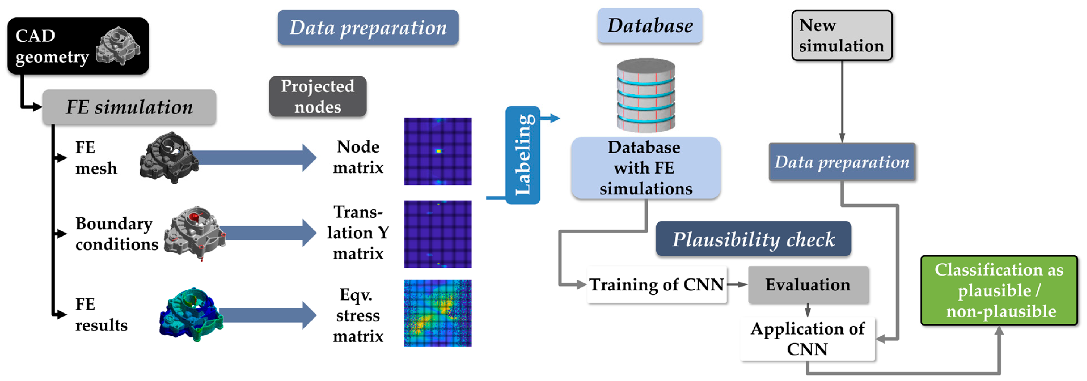
2. Methodical Approach

In order to provide conclusive answers to the questions raised, an overview of the planned examinations is presented. Overall, three different influencing factors are relevant to the general investigation: the classification realization, the dataset, and the CNN architecture. All three of these divisions have different influencing parameters that affect the overall result. The objective of the experiment is always the prediction of the plausibility cause, whether it is due to a faulty mesh, wrong load values, or unrealistic geometry parameters. Figure 5 provides an overview, and the following subsections present the different parts in more detail.

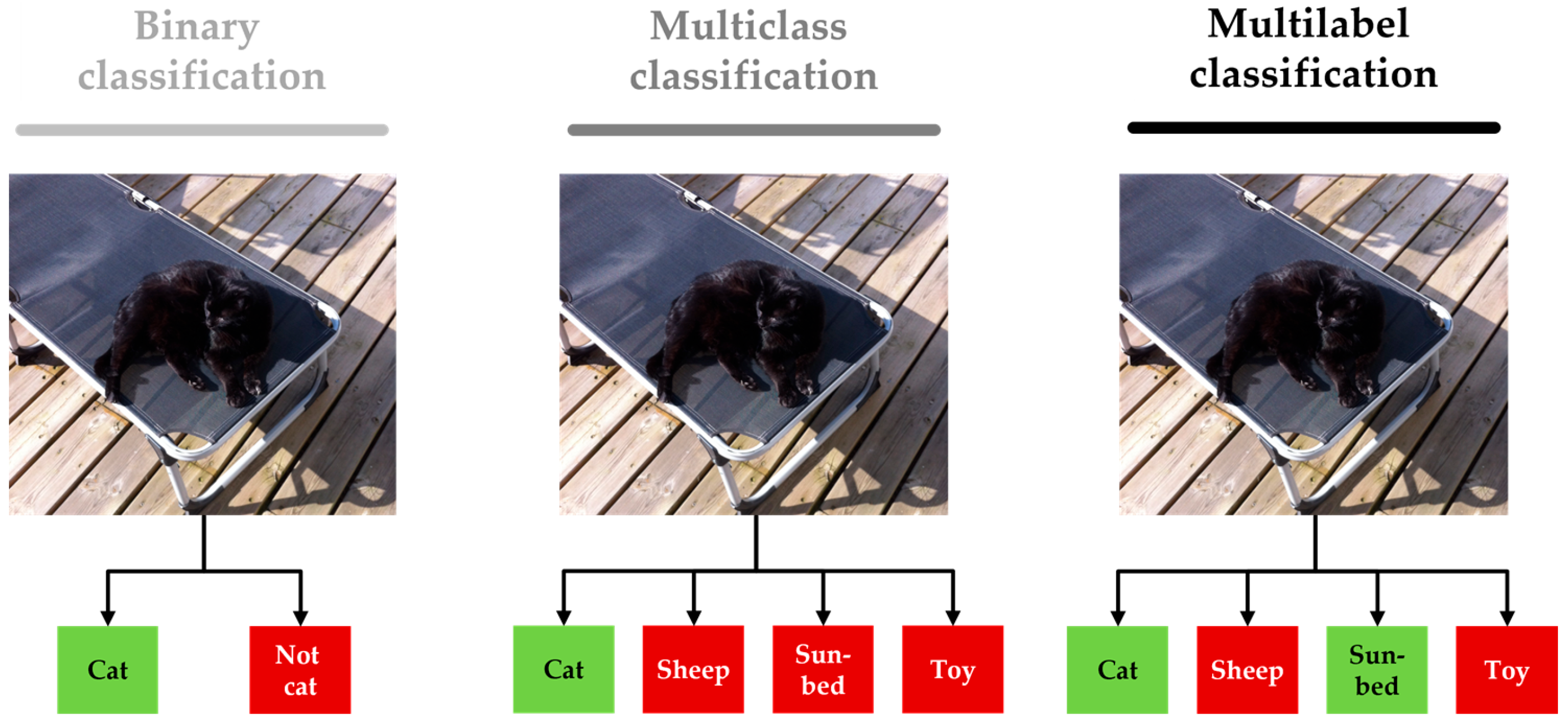
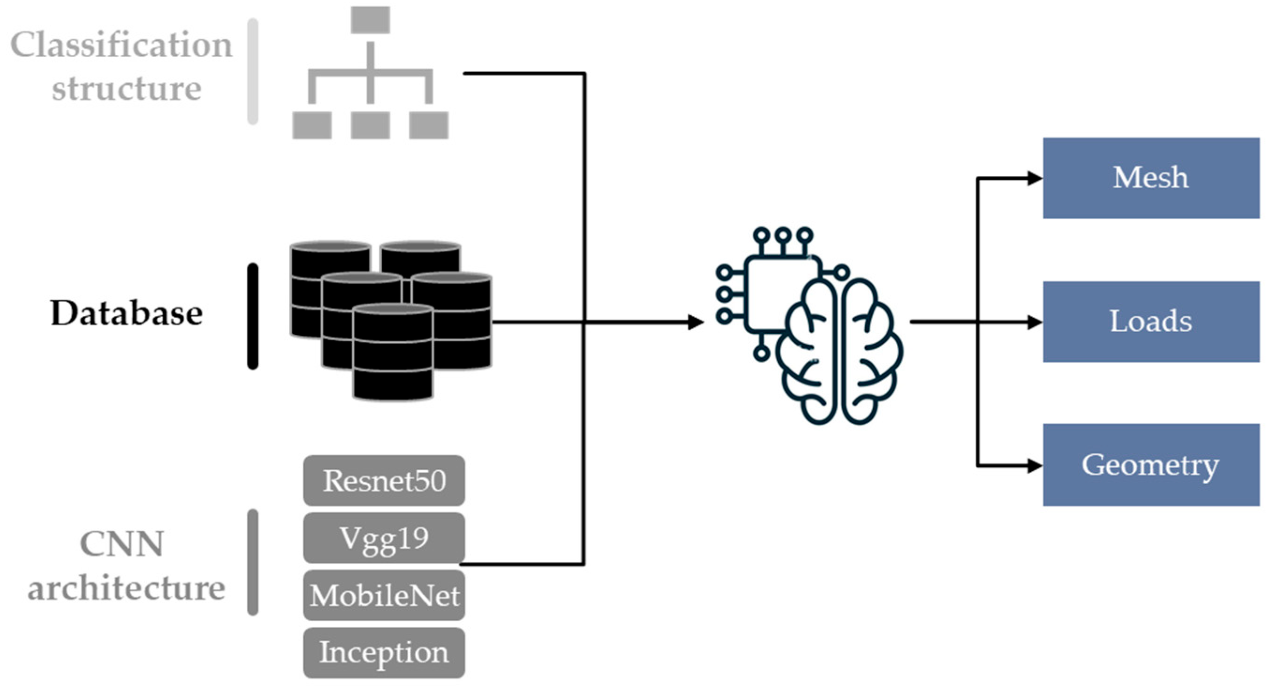
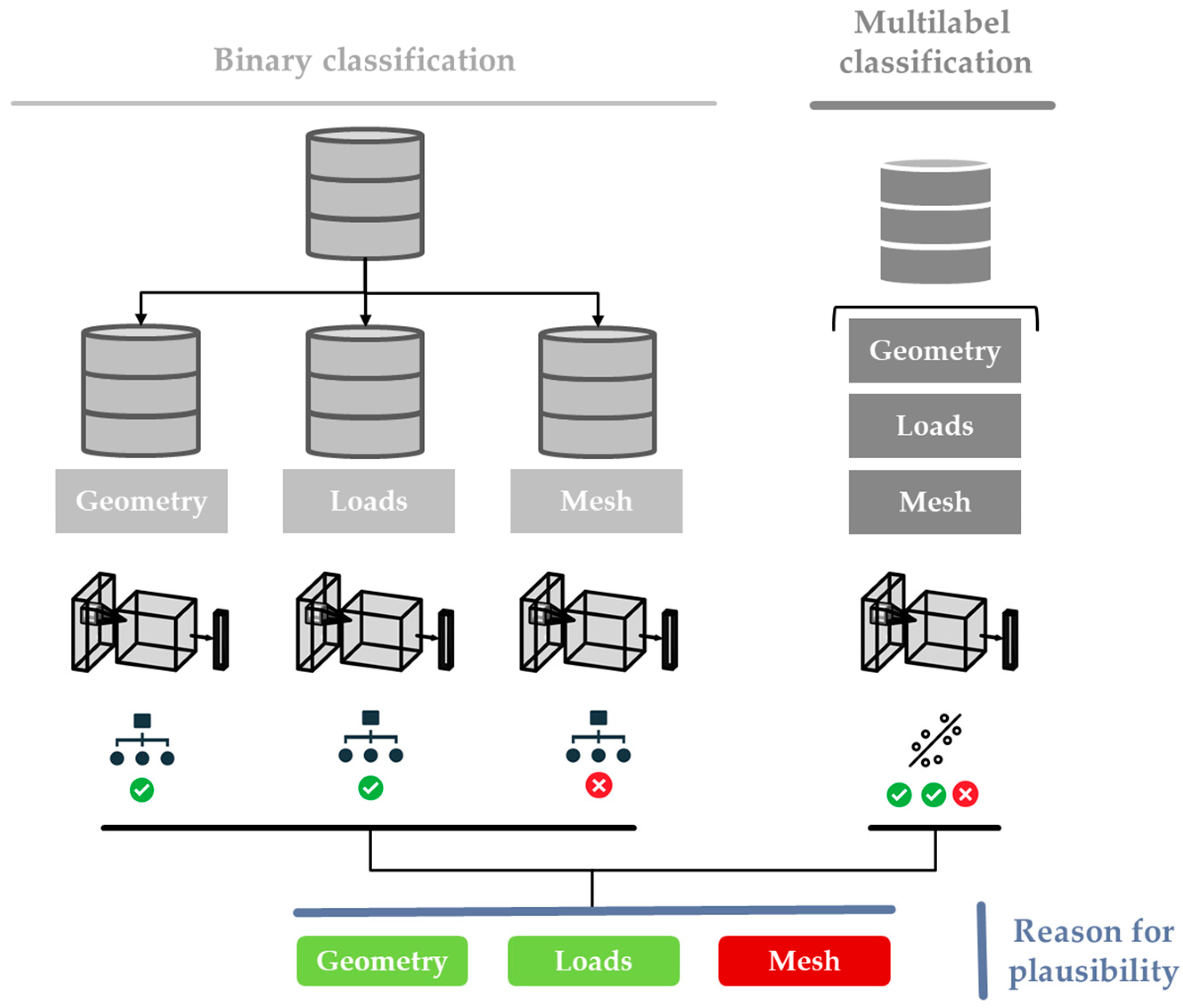
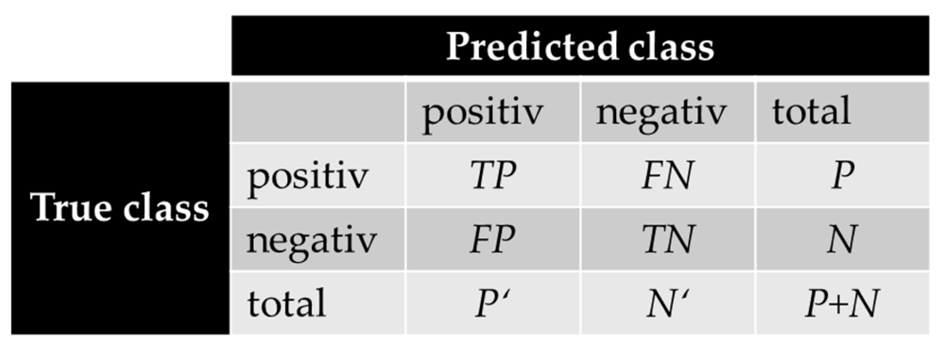
2.1. Classification Structure

First, the realization of the multilabel classification is explained in greater depth. Two implementation ideas were developed based on the theoretical knowledge from Section 1.2 and are shown schematically in Figure 6. The first concept applies several binary classifiers, each of which predicts one specific class. These consist of a CNN for classification and a dataset extracted from the entire simulation pool. In contrast, the second model uses a conversion of the problem into a regression model. For this purpose, the CNN structure is adapted correspondingly by replacing the softmax and classification layers with sigmoid and cross-entropy loss layers. For this application, the dataset does not require any further processing. The choice of CNN architecture is independent of the selected execution, although the binary classification theoretically offers the advantage of using different CNN models for each classifier.

The third possibility, adaptation of the multiclass classification, was not pursued further since all combinations must be defined as classes, which would correspond to eight (2³) labels. As a result, very few simulations can be assigned to some classes, such as in a the category in which all three plausibility causes are true. Furthermore, this procedure would become more and more complex to handle when adding further classes, since the number of new necessary classes scales with input classes to the power of two.

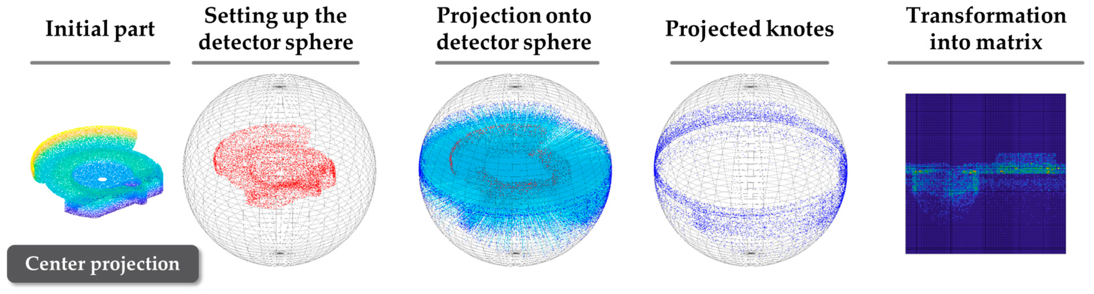
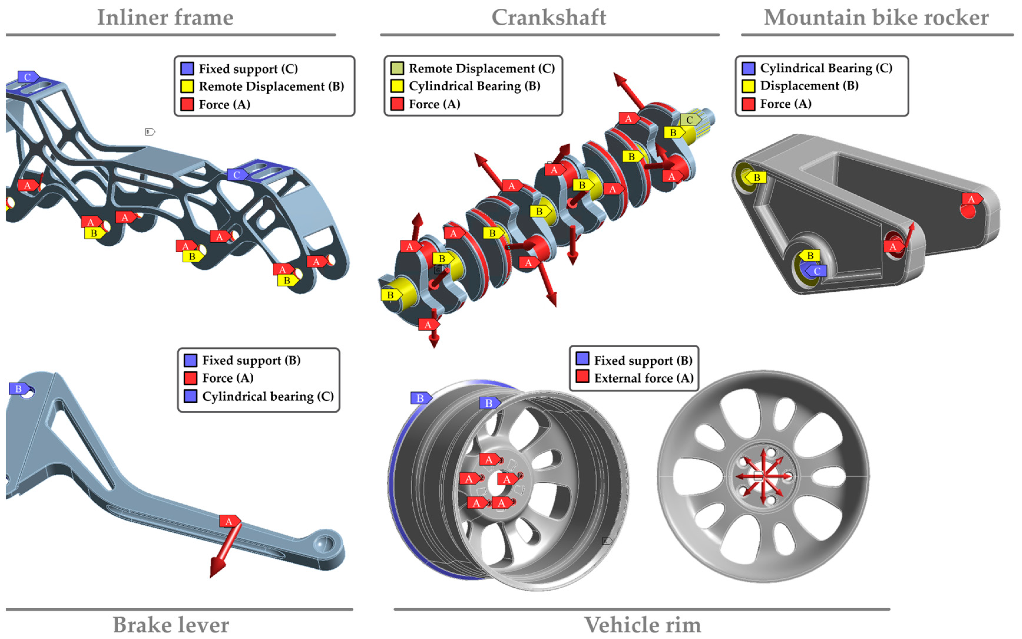
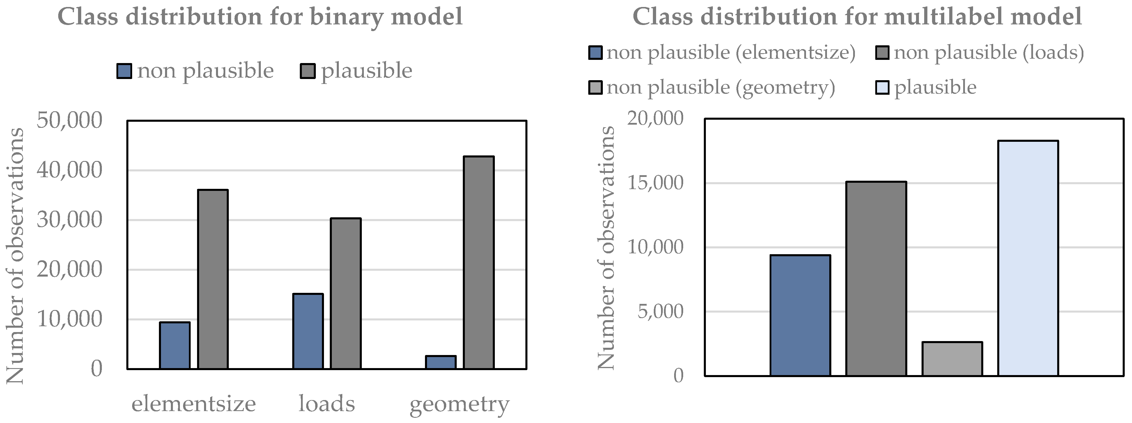
2.2. Database

In order to test and analyze the new approach, a large dataset with a sufficient number of simulations is necessary. Currently, only structural mechanics simulations with components are considered. The dataset includes already calculated simulations from previous publications [16,43]. The general structure of the entire dataset is organized with the help of the Opitz coding system [44]. The first digit of the code was selected as the distinguishing feature and the aim was to cover the existing categories as broadly as possible. The result with the corresponding simulation parts is listed in

Table 1. Categorization of the simulation parts in accordance with the Opitz coding system [44].

Rotatory			Non-Rotatory
L/D < 0.5	0.5 < L/D < 3	L/D ≥ 3	A/C > 4	A/B ≤ 3 & A/C ≥ 4	A/B ≤ 3	A/B ≤ 3 & A/C < 4
Vehicle rim		Crankshaft	Inliner frame		Brake lever	Mountain bike rocker

. The variables representing rotatory components stand for the length (L) and the diameter (D), while for the non-rotatory ones the maximum dimensions are sorted in all three directions in space and defined with A as the highest value and C as the lowest value.

In total, five components from different applications and domains are integrated into the entire dataset, all displayed in Figure 7. All simulations were calculated with parametric CAD models using Ansys Workbench (version 19.2 and 2021 R2). For generation of the results, parameter studies were performed with d-optimal experimental designs (DOE) for the different simulations [45]. After successful calculation of the FE simulation, an APDL script saves the results as a text file, including stresses, deformations, boundary conditions, and the general mesh.

The simulations were built using real loading conditions (inliner frame or mountain bike rocker) or information from the literature (crankshaft [46,47], brake lever [48], or car rim [49,50]). An overview of the various components and simulation setups is shown in Figure 7, with more detailed information on the simulations listed in [16,43].

For all simulations, the element size of the mesh, the load values, and the geometric variables of the component were used as parameters. These all affect the non-plausibility of FE simulations, and the goal is to detect these certain error sources. Since the focus of previous datasets was not differentiated by plausibility cause, the geometric non-plausibility cases were not taken into account in all parts. To close this gap and to test how the models behave with smaller datasets, supplementary studies focusing on geometric plausibility reasons were created for the vehicle rim and brake lever.

An overview of the calculated simulations and the labeled results is given in

Table 2. General information about the demonstrative study simulation datasets, with the numbers of the additional dataset in brackets.

Dataset	Simulation Numbers	Plausible	Non-Plausible Mesh	Non-Plausible Geometry	Non-Plausible Loads	Storage Space
Vehicle rim	9968	3736	2488	0	4992	676 GB
	(1816)	(80)	(792)	(1520)	(888)	217 GB
Brake lever	9862	5896	2493	0	1987	574 GB
	(1225)	(554)	(315)	(290)	(251)	64 GB
Bike rocker	22,624	12,257	3780	1620	6776	2890 GB
Crankshaft	8640	4800	1440	0	2880	6920 GB
Inliner frame	8952	4344	2172	0	3252	1650 GB
Whole dataset	63,087	31,667	13,480	3430	21,026	12,991 GB

. In total, over 63,000 simulations are in the dataset, corresponding to a storage requirement of almost 13 TB. Most simulations were calculated with the bike rocker and the smallest amount with the crankshaft. In the case of the vehicle rim and brake lever, the second study for the geometrical error cause is added below in brackets as it was calculated with a second DOE plan. The sum of the plausible and different non-plausible classes always exceeds the total number of simulations. This is due to the fact that several reasons for non-plausibility can exist per simulation. The table also shows that the geometrically non-plausible reason is the least represented in the data and accordingly forms an imbalanced dataset, which can thus lead to favoritism toward the majority class from the trained model. Labeling of each parameter study was performed by a combination of automatic (e.g., rule-based for high load values) and manual labeling.

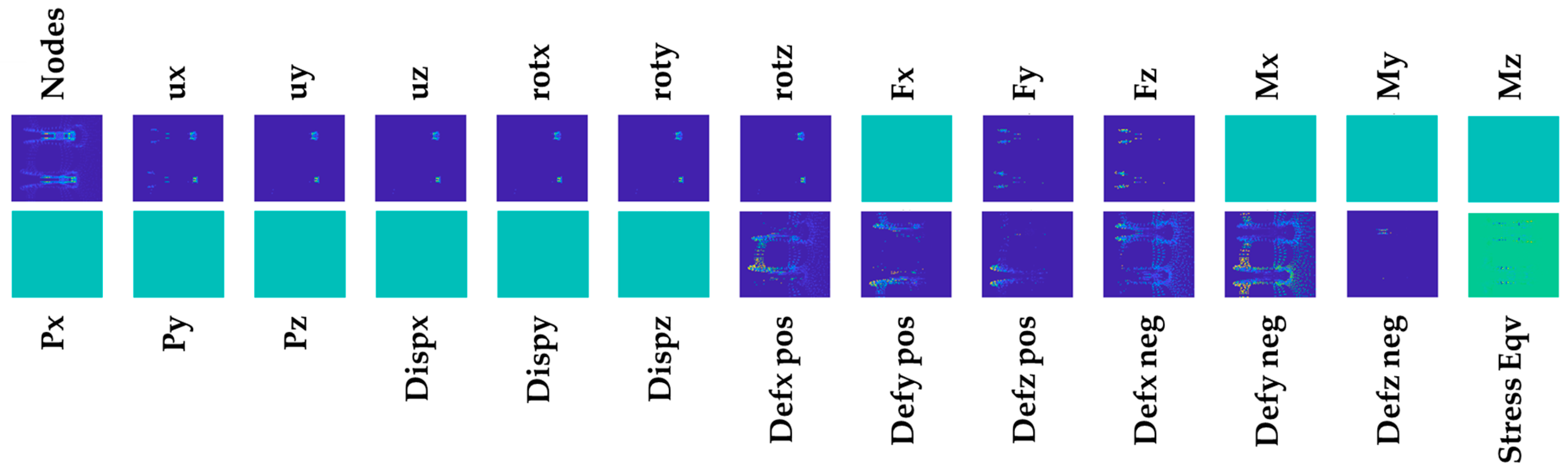
Dataset Preparation

After description and explanation of the available simulation pool, the next step is to demonstrate conversion of the simulation setup and results into matrices. The idea behind the transformation and arrangement of the matrices is to generate the “DNA of the simulation” and represent the simulation setup and results. An example transformation of a simulation is shown in Figure 8 including the input and result variables. With this investigation, the goal was to test a universal approach, which is the reason for including as many loads as possible in the matrix collection. The most common types of loads should be implemented, even if some of them are not part of the simulation pool. Consequently, 26 different matrices are created for one simulation: nodes, fixed translation and rotation in the X-, Y-, and Z-direction, force, external force and pressure in the X-, Y-, and Z-direction, moment around the X-, Y-, and Z-axis, the positive and negative displacements in the X-, Y- and Z-direction, and the equivalent von Mises stress. A resolution of 100 × 100 was chosen to generate the datasets for both classification approaches. The matrices are prepared through a special method of normalization, which is explained in detail in [16]. Through this process, the boundary conditions and result values are normalized differently in order to better represent FE simulations.

One additional advantage of projection conversion is the reduced storage space. After execution of the method, the matrices for the entire dataset only need about 10.5 GB compared to the original 13 TB. Of course, size depends on the resolution of the transformation, as the data requirements for higher resolution also increase. For this study, the dataset for each simulation parameter study was split 80/20 into training and testing data. As a result, 10% of the training dataset was selected for validation during training.

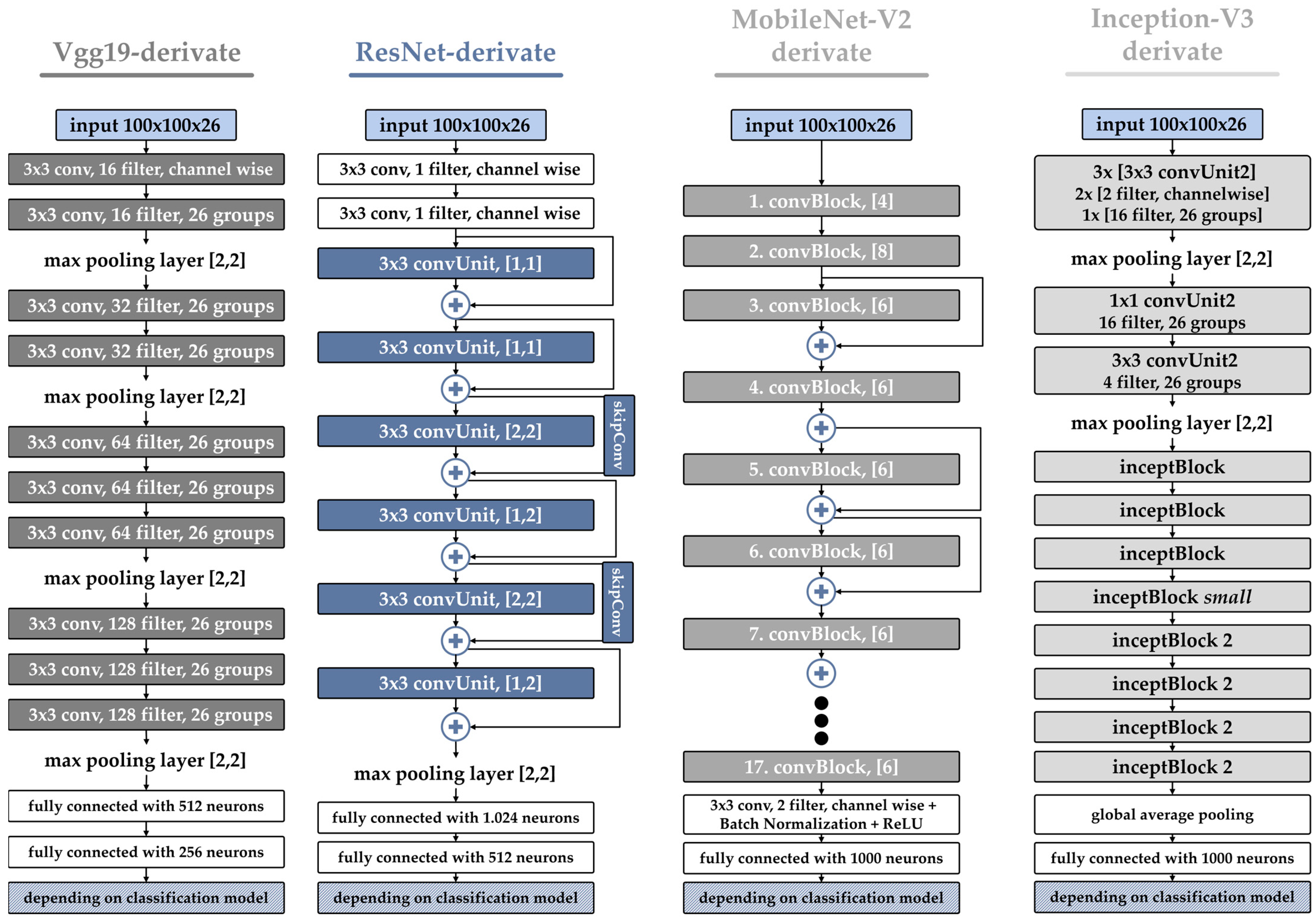
2.3. CNN Architecture

After explaining the classification procedure and the dataset, this chapter will focus on applied CNNs. A total of four architectures were investigated: Vgg19, ResNet, Inception-V3, and MobileNet-V2. Figure 9 shows a simplified comparison of the architectures. Due to the size of some architectures, the representation was simplified.

The Vgg19-derivate uses four groups of sequential convolution layers, each followed by a ReLU (Rectified Linear Unit) layer. Compared to the original Vgg19 architecture, a block of convolutional layers was removed due to the lower resolution of the matrix input. Furthermore, the number of filters per convolutional layer was reduced so a comparable batch size could be applied for all architectures. The variant derived from ResNet is shown in a simplified manner in Figure 9 using convUnits, each consisting of a convolution, batch normalization, ReLU activation, convolution, and batch normalization layer. The filter size is 3 × 3 for both convolution layers, and the values in the square brackets describe the number of filters and the stride for the layer. The two skipConv blocks contain extra convolution layers and are necessary for the results to have the same format when merging. The third architecture is based on MobileNet-V2 and is illustrated schematically via convBlock units in Figure 9. A convBlock contains a channel-wise convolution with 6 filters, batch normalization, an ReLU layer, channel-wise convolution with one filter, batch normalization, an ReLU layer, a channel-wise convolution layer with a fixed number of filters (matching the input to the convBlock), and a batch normalization layer. A total of 17 blocks are arranged one after the other with partial skip paths, modeled after the original MobileNet-V2. For the adapted Inception-V3 network, the first layers were replaced by convUnit2 blocks, each composed of a convolution, batch normalization, and ReLU layer, with the convolution parameters listed in the square brackets. The following inceptBlock modules are carried over from the original Inception-V3 architecture and contain four threads each with different convolution, batch normalization, ReLU, and pooling layers, as shown in Figure 4. Due to the lower resolution of the input, the last two larger inception blocks were removed from the network.

For all models, the last three layers depend on the classification model. In the case of binary classification, they are a fully connected layer with two neurons and a softmax and classification layer. In contrast, in the multilabel instance, a fully connected layer with three neurons and a sigmoid and cross-entropy loss layer is applied.

The evaluation metric for comparison of the different approaches and models is usually classification accuracy. This metric is derived from the confusion matrix and is calculated for the three datasets: the training dataset, validation dataset, and test dataset. A confusion matrix with the associated variable names is shown in Figure 10, with the variables True Positive (TP), True Negative (TN), False Positive (FP), and False Negative (FN).

For a balanced dataset, classifications accuracy is often applied, which can be calculated according to [52,53]:

$$accuracy=\frac{TP+TN}{TP+TN+FP+FN}$$

However, this metric is not appropriate for the evaluation of imbalanced datasets since it does not consider the uneven distribution of classes. An alternative is the balanced accuracy from [51]:

$$balanced accuracy=\frac{1}{2}\left(\frac{TP}{TP+FN}+\frac{TN}{TN+FP}\right)$$

Another metric for imbalanced datasets is the G-Mean (geometric mean) value defined by [54]:

$$G-Mean=\sqrt{\frac{TP}{TP+FN}·\frac{TN}{TN+FP}}$$

Besides the presented metrics, many others have been developed, such as the F-Measure, the Receiver Operator Curve (ROC), the area under the curve (AUC), the Precision Recall (PR) Diagram, and the Index of Balanced Accuracy (IBA), which are explained in detail in [51,54,55,56].

3. Result Comparison

After explanation of the different classification adaptations and CNN architectures, the following chapter examines them in further depth using the described evaluation metrics. All models were trained on the same computational server, which had two AMD EPYC 7643 processors, 256 GB RAM, and two Nvidia A40 (46 GB) graphics cards installed. The basic set of training parameters is identical for all models, as shown in

Table 3. Training parameters for the CNN models.

Options	Value
Solver Type	adam
Mini Batchsize	128
Max. Epochs	40
Validation Frequency	125
Validation Patience	8
Shuffle	Once
Learning Rate Binary	MobileNet: 0.0001 ResNet: 0.000001 Vgg19: 0.00001 Inception: 0.001
Learning Rate Multilabel	MobileNet: 0.0001 ResNet: 0.000001 Vgg19: 0.00001 Inception: 0.0001

. Only the learning rate was adjusted for different models because a uniform rate did not work. Data was divided into training, validation, and test datasets automatically according to the 72%–8%–20% principle and was performed in the same manner for all datasets and models.

Class distribution for the two variants of training data is shown in Figure 11. The number of non-plausible classes is identical for both cases, with only the plausible instances varying. Since only one cause of error is detected in the binary classifiers, the other two non-plausible cases are still included as plausible. All training datasets consist of 45,444 observations for training. The uneven distribution of classes is particularly evident in the geometry class. Therefore, the metrics balanced accuracy and G-Mean are applied for evaluation to account for the non-uniformity of the distribution.

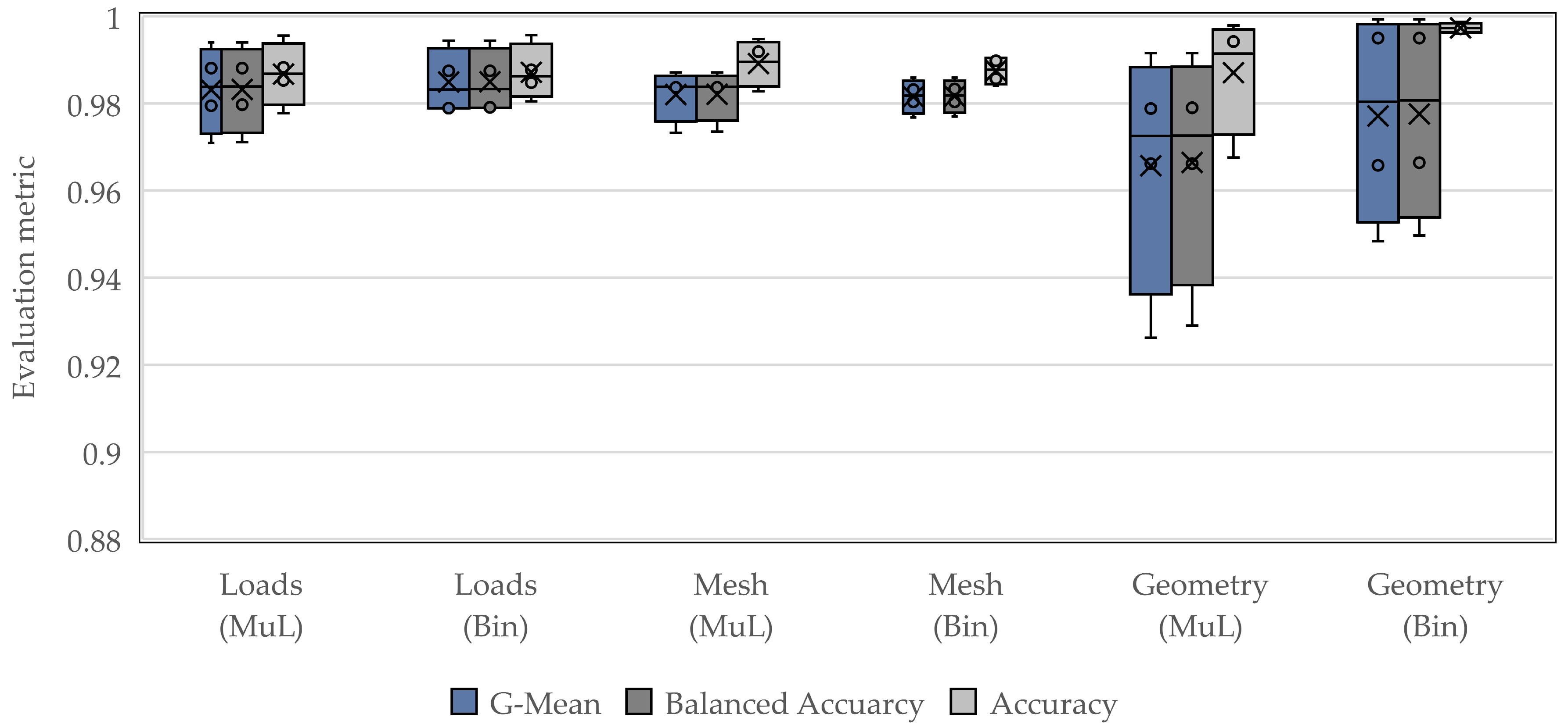
3.1. Classification Approach

For initial comparison of the classification models, the results of all CNN models were analyzed for all three classes. The derivatives of Vgg19, ResNet, Inception-V3, and MobileNet-V2 serve as the CNN models.

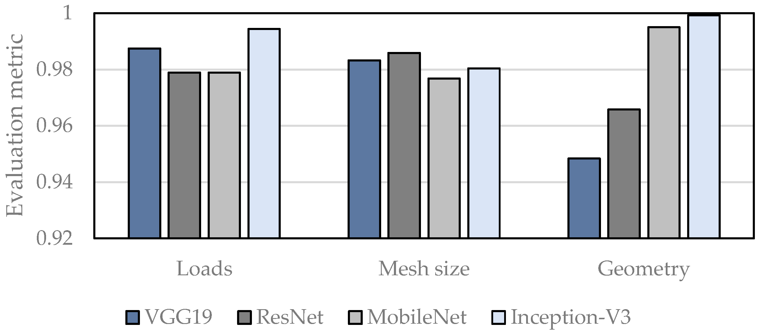
The results are shown in the diagram in Figure 12. The training duration of the CNN models varied between 4 h and 12 h. The plot shows the test results for the error classes in the binary (Bin) and multilabel (MuL) approaches. The boxplot is composed of all four CNN architectures, with all detailed results listed in the Appendix A in

Table A1. All classification results for the binary models and different CNN architectures.

	Dataset Binary			Evaluation Metric
	Loads	Mesh Size	Geometry
Vgg19	0.9875	0.9832	0.9484	G-Mean
	0.9875	0.9833	0.9497	Balanced Accuracy
	0.9877	0.9906	0.9960	Accuracy
ResNet	0.9789	0.9859	0.9658	G-Mean
	0.9791	0.9859	0.9664	Balanced Accuracy
	0.9848	0.9898	0.9971	Accuracy
MobileNet-V2	0.9789	0.9768	0.9950	G-Mean
	0.9789	0.9770	0.9950	Balanced Accuracy
	0.9805	0.9857	0.9976	Accuracy
Inception-V3	0.9944	0.9804	0.9993	G-Mean
	0.9944	0.9804	0.9993	Balanced Accuracy
	0.9957	0.9840	0.9987	Accuracy

and

Table A2. All classification results for the multilabel models and different CNN architectures.

	Dataset Multilabel			Evaluation Metric
	Loads	Mesh Size	Geometry
Vgg19	0.9709	0.9733	0.9262	G-Mean
	0.9711	0.9735	0.9290	Balanced Accuracy
	0.9778	0.9828	0.9942	Accuracy
ResNet	0.9795	0.9871	0.9662	G-Mean
	0.9797	0.9871	0.9662	Balanced Accuracy
	0.9853	0.9919	0.9676	Accuracy
MobileNet-V2	0.9881	0.9840	0.9788	G-Mean
	0.9881	0.9840	0.9790	Balanced Accuracy
	0.9883	0.9871	0.9979	Accuracy
Inception-V3	0.9940	0.9837	0.9916	G-Mean
	0.9940	0.9837	0.9916	Balanced Accuracy
	0.9956	0.9948	0.9886	Accuracy

. The scores for all methods are generally very high, with all results above 0.9. Comparison of the G-Mean and balanced accuracy values indicates that scatter is lower for the binary methods over all plausibility causes.

Analysis of the highest classification results also reveals that the binary and multilabel variants achieve nearly identical results for the loads and mesh classes. The absolute differences are very small, in some cases in the third decimal digit. Only in the geometry class is the higher accuracy of the binary classification visible. In evaluation of the geometry cause, it is evident that this class was the most challenging in the classification, recognizable by the high dispersion of both classification variants.

Because of low dispersion and higher accuracy for the geometry class of the binary classifiers, they will be examined in more detail. The aim is to compare the different CNN architectures against each other in order to obtain the best results.

3.2. CNN Architecture

The bar chart in Figure 13 compares the calculated results. In general, the G-Mean values achieved by the respective architectures are very high, and the distribution per class is low in most cases. It is also evident that the geometry class had the most deviations, which is due to the imbalance of the dataset. Furthermore, it is visible that the Inception-V3 derivative best classified the loads and geometry. For the plausibility cause mesh size, ResNet achieved the highest accuracy. The Vgg19 architecture also obtained very high results in the first two classes, though not for the geometric error reason. Here, MobileNet could score very high values, whereas it performed worse in comparison to the other two classes.

Since the Inception network performed the best overall, another study with individual class weights was carried out. For each binary classifier, individual weights were determined depending on the class distribution. Afterwards, the networks were trained again with an adapted learning rate of 0.0005 and the results were compared, which are shown in the confusion matrix in Figure 14. The G-Mean values achieved are as follows: 0.9930 (Loads), 0.9866 (Mesh), and 0.9978 (geometry).

The results show that accuracy could again be improved by weighted classes but on a smaller scale, which is inevitable due to the already very high values. Above all, the mesh class was further enhanced, whereas the other two plausibility causes marginally worsened.

4. Discussion

After presentation of the obtained results, it can be concluded that both classification approaches are suitable for the application of specific plausibility cause detection in FE simulations. This answers the first research question as both presented classification approaches provide very good results, and principal detection of the cause of the error is possible with both of them. However, a detailed comparison of the two approaches reveals the different advantages and disadvantages of the procedures.

The advantage of multilabel classification via an adapted regression model is the reduced training time since only one model needs to be trained instead of three in the case of binary classification. Therefore, the model can theoretically be adapted to a new dataset faster. Furthermore, integration of all three labels into the dataset reduces class imbalance compared to a plain binary classifier, as can be seen in Figure 11. Nevertheless, training also showed that there was high sensitivity to the appropriate choice of hyper parameters, which made the training time-consuming in some cases.

In contrast, the advantage of binary classifiers lies in the learning of a specific problem, which thus allows it to predict that problem with higher accuracy at the expense of training time. Additionally, they are much more flexible since the CNN architecture can be chosen specifically for the class. In the case of application as an assistance system for plausibility checking in industry, new data could be brought into the system more easily because only the recognition of an error would cause temporarily interruption.

In addition to the multilabel concept comparison, it is noticeable when comparing the CNN architectures that all networks achieve very good results. However, to answer the second research question, the Inception-V3 adaptation achieves especially high classification results. The other three network types mostly have their strengths in a certain class and are less capable of detecting the other two. The use of specific class weights resulted in a further general improvement, which leads to the conclusion that the combination of binary classifiers with the Inception-V3 network is best suited for the dataset and the application task at hand.

5. Conclusions and Outlook

In summary, this paper tested multilabel classification approaches with different networks to predict the specific plausibility cause. For this purpose, a dataset with over 60,000 simulations was prepared and given as input to different CNNs. The achieved accuracies were reasonably high, which thus allows for the conclusion that a prediction of more accurate error causes in FE simulations is possible.

The next steps could address the analysis of the input vector in more depth. In this paper, the matrices were chosen to ensure that the procedure was generally applicable, although exploring the exact influence of the different matrices on recognition accuracy would be very interesting. In addition, other network architectures and newer Neural Network types (such as Visual Transformer [57]) could be adapted and used for classification. Furthermore, methods from the field of data augmentation could be applied in different ways to reduce the imbalance of the classes. Finally, other causes for non-plausible simulations could be taken into account and the database could be enhanced accordingly.

References

- Feng, Y.; Zhao, Y.; Zheng, H.; Li, Z.; Tan, J. Data-driven product design toward intelligent manufacturing: A review. Int. J. Adv. Robot. Syst. 2020, 17, 1729881420911257. [Google Scholar] [CrossRef]
- Briard, T.; Jean, C.; Aoussat, A.; Véron, P.; Le Cardinal, J.; Wartzack, S. Data-driven design challenges in the early stages of the product development process. Proc. Des. Soc. 2021, 1, 851–860. [Google Scholar] [CrossRef]
- Quan, H.; Li, S.; Zeng, C.; Wei, H.; Hu, J. Big Data driven Product Design: A Survey. arXiv 2021, arXiv:2109.11424. [Google Scholar]
- Iriondo, A.; Oscarsson, J.; Jeusfeld, M.A. Simulation Data Management in a Product Lifecycle Management Context. In Advances in Manufacturing Technology XXXI; IOS Press: Amsterdam, The Netherlands, 2017; pp. 476–481. [Google Scholar]
- Chari, S. Addressing Engineering Simulation Data Management (SDM) Challenges: How Engineering Enterprises Can Improve Productivity, Collaboration and Innovation; Cabot Partners Group, Inc.: Danbury, CT, USA, 2013. [Google Scholar]
- Yang, X.; Liang, J.; Liao, Y.; Liu, F.; Feng, X.; Wen, Y. Study of Universal Simulation Data Management System. In Proceedings of the 2009 International Conference on Information Technology and Computer Science, Kiev, Ukraine, 25–26 July 2009; pp. 333–338. [Google Scholar]
- Bennet, J.; Creary, L.; Englemore, R.; Melosh, R. SACON: A Knowledge-Based Consultant for Structural Analysis; Stanford Heuristic Programming Project; Stanford University—Computer Science Department: Stanford, CA, USA, 1979. [Google Scholar]
- Johansson, J. Manufacturability Analysis Using Integrated KBE, CAD and FEM. In Volume 5: 13th Design for Manufacturability and the Lifecycle Conference; 5th Symposium on International Design and Design Education; 10th International Conference on Advanced Vehicle and Tire Technologies; ASMEDC: Houston, TX, USA, 2008; pp. 191–200. [Google Scholar]
- Javadi, A.A.; Mehravar, M.; Faramarzi, A.; Ahangar-Asr, A. An artificial intelligence based finite element method. Comput. Intell. Syst. 2009, 1, 1–120. [Google Scholar]
- Lai, J.-Y.; Wang, M.-H.; Song, P.-P.; Hsu, C.-H.; Tsai, Y.-C. Recognition and decomposition of rib features in thin-shell plastic parts for finite element analysis. Comput. -Aided Des. Appl. 2018, 15, 264–279. [Google Scholar] [CrossRef]
- Song, P.-P.; Lai, J.-Y.; Tsai, Y.-C.; Hsu, C.-H. Automatic recognition and suppression of holes on mold bases for finite element applications. Eng. Comput. 2019, 35, 925–944. [Google Scholar] [CrossRef]
- Boussuge, F.; Léon, J.-C.; Hahmann, S.; Fine, L. Idealized models for FEA derived from generative modeling processes based on extrusion primitives. Eng. Comput. 2015, 31, 513–527. [Google Scholar] [CrossRef]
- Kestel, P.; Kügler, P.; Zirngibl, C.; Schleich, B.; Wartzack, S. Ontology-based approach for the provision of simulation knowledge acquired by Data and Text Mining processes. Adv. Eng. Inform. 2019, 39, 292–305. [Google Scholar] [CrossRef]
- Zimmerling, C.; Poppe, C.; Kärger, L. Virtuelle Produktentwicklung mittels Simulationsmethoden und KI. Lightweight Des. 2019, 12, 12–19. [Google Scholar] [CrossRef]
- Spruegel, T.C.; Hallmann, M.; Wartzack, S. A concept for FE plausibility checks in structural mechanics. In Proceedings of the NAFEMS World Congress, San Diego, CA, USA, 21–24 June 2015. [Google Scholar]
- Spruegel, T.C.; Bickel, S.; Schleich, B.; Wartzack, S. Approach and application to transfer heterogeneous simulation data from finite element analysis to neural networks. J. Comput. Des. Eng. 2021, 8, 298–315. [Google Scholar] [CrossRef]
- Bickel, S.; Spruegel, T.C.; Schleich, B.; Wartzack, S. How Do Digital Engineering and Included AI Based Assistance Tools Change the Product Development Process and the Involved Engineers. Proc. Int. Conf. Eng. Des. 2019, 1, 2567–2576. [Google Scholar] [CrossRef]
- Bonaccorso, G. Machine Learning Algorithms, 1st ed.; Packt Publishing Limited: Birmingham, UK, 2017. [Google Scholar]
- Mahesh, B. Machine learning algorithms—A review. Int. J. Sci. Res. 2020, 9, 381–386. [Google Scholar]
- Goodfellow, I.; Courville, A.; Bengio, Y. Deep Learning; The MIT Press: Cambridge, MA, USA, 2016. [Google Scholar]
- Cleve, J.; Lämmel, U. Data Mining, 2nd ed.; De Gruyter Oldenbourg: Berlin, Germany, 2016. [Google Scholar]
- Runkler, T.A. Data Mining: Methoden und Algorithmen Intelligenter Datenanalyse, 1st ed.; mit 7 Tabellen; Vieweg + Teubner: Wiesbaden, Germany, 2010. [Google Scholar]
- Tsoumakas, G.; Katakis, I. Multi-Label Classification. Int. J. Data Warehous. Min. 2007, 3, 1–13. [Google Scholar] [CrossRef]
- Read, J.; Pfahringer, B.; Holmes, G.; Frank, E. Classifier chains for multi-label classification. Mach. Learn. 2011, 85, 333–359. [Google Scholar] [CrossRef]
- Deng, L. Deep Learning: Methods and Applications. FNT Signal Process. 2014, 7, 197–387. [Google Scholar] [CrossRef]
- Janiesch, C.; Zschech, P.; Heinrich, K. Machine learning and deep learning. Electron Mark. 2021, 31, 685–695. [Google Scholar] [CrossRef]
- LeCun, Y.; Bengio, Y.; Hinton, G. Deep learning. Nature 2015, 521, 436–444. [Google Scholar] [CrossRef]
- LeCun, Y.; Boser, B.; Denker, J.S.; Henderson, D.; Howard, R.E.; Hubbard, W.; Jackel, L.D. Backpropagation Applied to Handwritten Zip Code Recognition. Neural Comput. 1989, 1, 541–551. [Google Scholar] [CrossRef]
- LeCun, Y.; Bottou, L.; Bengio, Y.; Haffner, P. Gradient-based learning applied to document recognition. Proc. IEEE 1998, 86, 2278–2324. [Google Scholar] [CrossRef]
- Krizhevsky, A. Learning Multiple Layers of Features from Tiny Images; University of Toronto: Toronto, ON, USA, 2009. [Google Scholar]
- Everingham, M.; van Gool, L.; Williams, C.K.I.; Winn, J.; Zisserman, A. The Pascal Visual Object Classes (VOC) Challenge. Int. J. Comput. Vis. 2010, 88, 303–338. [Google Scholar] [CrossRef]
- Deng, J.; Dong, W.; Socher, R.; Li, L.-J.; Li, K.; Fei-Fei, L. ImageNet: A large-scale hierarchical image database. In Proceedings of the 2009 IEEE Conference on Computer Vision and Pattern Recognition, Miami, FL, USA, 20–25 June 2009. [Google Scholar]
- Krizhevsky, A.; Sutskever, I.; Hinton, G.E. ImageNet classification with deep convolutional neural networks. Commun. ACM 2017, 60, 84–90. [Google Scholar] [CrossRef]
- Simonyan, K.; Zisserman, A. Very Deep Convolutional Networks for Large-Scale Image Recognition. arXiv 2014, arXiv:1409.1556. [Google Scholar]
- Srivastava, R.K.; Greff, K.; Schmidhuber, J. Highway Networks. arXiv 2015, arXiv:1505.00387. [Google Scholar]
- He, K.; Zhang, X.; Ren, S.; Sun, J. Deep Residual Learning for Image Recognition. In Proceedings of the IEEE Conference on Computer Vision and Pattern Recognition (CVPR), Las Vegas, NV, USA, 27–30 June 2016. [Google Scholar]
- Szegedy, C.; Liu, W.; Jia, Y.; Sermanet, P.; Reed, S.; Anguelov, D.; Erhan, D.; Vanhoucke, V.; Rabinovich, A. Going deeper with convolutions. In Proceedings of the 2015 IEEE Conference on Computer Vision and Pattern Recognition (CVPR), Boston, MA, USA, 7–12 June 2015. [Google Scholar]
- Szegedy, C.; Ioffe, S.; Vanhoucke, V.; Alemi, A. Inception-v4, Inception-ResNet and the Impact of Residual Connections on Learning. In Proceedings of the AAAI Conference on Artificial Intelligence, San Francisco, CA, USA, 4–9 February 2017; Volume 31. [Google Scholar]
- Huang, G.; Liu, Z.; van der Maaten, L.; Weinberger, K.Q. Densely Connected Convolutional Networks. In Proceedings of the IEEE Conference on Computer Vision and Pattern Recognition, Honolulu, HI, USA, 21–26 July 2017. [Google Scholar]
- Howard, A.G.; Zhu, M.; Chen, B.; Kalenichenko, D.; Wang, W.; Weyand, T.; Andreetto, M.; Adam, H. MobileNets: Efficient Convolutional Neural Networks for Mobile Vision Applications. arXiv 2017, arXiv:1704.04861. [Google Scholar]
- Sandler, M.; Howard, A.; Zhu, M.; Zhmoginov, A.; Chen, L.-C. MobileNetV2: Inverted Residuals and Linear Bottlenecks. In Proceedings of the 2018 IEEE/CVF Conference on Computer Vision and Pattern Recognition, Salt Lake City, UT, USA, 18–22 June 2018. [Google Scholar]
- Howard, A.; Sandler, M.; Chen, B.; Wang, W.; Chen, L.-C.; Tan, M.; Chu, G.; Vasudevan, V.; Zhu, Y.; Pang, R.; et al. Searching for MobileNetV3. In Proceedings of the 2019 IEEE/CVF International Conference on Computer Vision (ICCV), Seoul, Korea, 27 October–2 November 2019. [Google Scholar]
- Bickel, S.; Schleich, B.; Wartzack, S. Resnet networks for plausibility detection in finite element simulations. In Proceedings of the DS 118: Proceedings of NordDesign 2022, Copenhagen, Denmark, 16–18 August 2022; pp. 1–10. [Google Scholar]
- Opitz, H. A Classification System to Describe Workpieces; Taylor, A., Translator; Pergamon Press: New York, NY, USA, 1970. [Google Scholar]
- Murray-Smith, D.J. Testing and Validation of Computer Simulation Models: Principles, Methods and Applications, 1st ed.; Springer International Publishing: Cham, Switzerland, 2015. [Google Scholar]
- Van Basshuysen, R. Handbuch Verbrennungsmotor: Grundlagen, Komponenten, Systeme, Perspektiven, 7th ed.; mit 1804 Abbildungen und mehr als 1400 Literaturstellen; Springer Vieweg: Wiesbaden, Germany, 2015. [Google Scholar]
- Kohler, E. Verbrennungsmotoren: Motormechanik, Berechnung und Auslegung des Hubkolbenmotors, 4th ed.; Friedr. Vieweg & Sohn Verlag: Wiesbaden, Germany, 2006. [Google Scholar]
- DIN. Cycles—Safety Requirements for Bicycles—Part 4: Braking Test Methods; German Institute for Standardization e.V.: Berlin, Germany, 2014. [Google Scholar]
- Wang, L.; Chen, Y.; Wang, C.; Wang, Q. Fatigue Life Analysis of Aluminum Wheels by Simulation of Rotary Fatigue Test. SV-JME 2011, 57, 31–39. [Google Scholar] [CrossRef]
- Jape, R.K.; Jadhav, S.G.; Student, M.T. CAD modeling and FEA analysis of wheel rim for weight reduction. Int. J. Eng. Sci. Comput. 2016, 6, 7404–7411. [Google Scholar]
- Brodersen, K.H.; Ong, C.S.; Stephan, K.E.; Buhmann, J.M. The Balanced Accuracy and Its Posterior Distribution. In Proceedings of the 2010 20th International Conference on Pattern Recognition, Washington, DC, USA, 23–26 August 2010. [Google Scholar]
- Fawcett, T. An introduction to ROC analysis. Pattern Recognit. Lett. 2006, 27, 861–874. [Google Scholar] [CrossRef]
- Powers, D.M.W. Evaluation: From precision, recall and F-measure to ROC, informedness, markedness and correlation. arXiv 2020, arXiv:2010.16061. [Google Scholar]
- Branco, P.; Torgo, L.; Ribeiro, R. A Survey of Predictive Modelling under Imbalanced Distributions. arXiv 2015, arXiv:1505.01658. [Google Scholar]
- García, V.; Mollineda, R.A.; Sánchez, J.S. Index of Balanced Accuracy: A Performance Measure for Skewed Class Distributions; Springer: Berlin/Heidelberg, Germany, 2009; pp. 441–448. [Google Scholar]
- Sun, Y.; Wong, A.K.C.; Kamel, M.S. Classification of imbalanced data: A review. Int. J. Patt. Recogn. Artif. Intell. 2009, 23, 687–719. [Google Scholar] [CrossRef]
- Dosovitskiy, A.; Beyer, L.; Kolesnikov, A.; Weissenborn, D.; Zhai, X.; Unterthiner, T.; Dehghani, M.; Minderer, M.; Heigold, G.; Gelly, S.; et al. An Image is Worth 16x16 Words: Transformers for Image Recognition at Scale. arXiv 2020, arXiv:2010.11929. [Google Scholar]