Robustness of Single- and Dual-Energy Deep-Learning-Based Scatter Correction Models on Simulated and Real Chest X-rays

Abstract

Chest X-rays (CXRs) represent the first tool globally employed to detect cardiopulmonary pathologies. These acquisitions are highly affected by scattered photons due to the large field of view required. Scatter in CXRs introduces background in the images, which reduces their contrast. We developed three deep-learning-based models to estimate and correct scatter contribution to CXRs. We used a Monte Carlo (MC) ray-tracing model to simulate CXRs from human models obtained from CT scans using different configurations (depending on the availability of dual-energy acquisitions). The simulated CXRs contained the separated contribution of direct and scattered X-rays in the detector. These simulated datasets were then used as the reference for the supervised training of several NNs. Three NN models (single and dual energy) were trained with the MultiResUNet architecture. The performance of the NN models was evaluated on CXRs obtained, with an MC code, from chest CT scans of patients affected by COVID-19. The results show that the NN models were able to estimate and correct the scatter contribution to CXRs with an error of <5%, being robust to variations in the simulation setup and improving contrast in soft tissue. The single-energy model was tested on real CXRs, providing robust estimations of the scatter-corrected CXRs.

1. Introduction

Chest X-ray radiography (CXR) is usually the first imaging technique employed to perform the early diagnosis of cardiopulmonary diseases. Typical pathologies detected in CXRs include pneumonia, atelectasis, consolidation, pneumothorax, and pleural and pericardial effusion [1]. Since the COVID-19 pandemic started in 2020, it has also been used as a tool to detect and assess the evolution of pneumonia caused by this condition [2]. CXR is used worldwide thanks to the simplicity with which it can be completed, the low cost, low radiation dose, and its sensitivity [3,4].

Regarding the position and orientation of the patient in relation to the X-ray source, the desired and most frequently used setup is posteroanterior (PA) projection [5] since it provides better visualization of the lungs [6]. However, this configuration requires the patient to be standing erect, which is not possible for critically ill patients, intubated patients, or some elderly people [6,7]. In these situations, it is more convenient to carry out anteroposterior (AP) projection, in which the patient can be sitting up in bed or lying in a supine position. Thus, AP images can also be acquired with a portable X-ray unit outside the radiology department when, due to the patient’s condition, it is advised not to shift him/her [6].

X-ray imaging is based on the attenuation that photons suffer when they traverse the human body so that photons that cross the body and reach the detector without interacting with the media, i.e., primary photons, form the image [8]. However, some photons interact with the media and are not absorbed but scattered. This secondary radiation can also reach the detector, representing background noise and causing a blurring in the primary image and considerable loss in the contrast-to-noise ratio (CNR) [9]. This effect is especially relevant in CXR due to the requirement of large detectors (at least 35 cm wide) to be able to cover the whole region of interest (ROI) [10]. To overcome this problem, several techniques have been proposed, which can be split into two types: Scatter suppression and scatter estimation [11]. Scatter suppression methods aim to remove, or at least reduce, the scattered photons that arrive at the detector, while scatter estimation methods try to obtain only the signal of the secondary photons and then subtract it from the total projection.

The most widely used scatter correction method is the anti-scatter grid, where a grid is interposed between the patient and the detector so that scattered photons are absorbed, while primary photons are allowed to pass [7,12]. This technique is successfully implemented in clinical practice [10] since many clinical systems incorporate this grid [13], although it has some disadvantages. First, an anti-scatter grid can also attenuate primary radiation, leading to noisy images [9,10]. Additionally, it can generate grid line artifacts in the image [14], and it can increase the radiation exposure between two and five times [5,15]. Finally, in AP acquisitions, it is difficult to accurately align the grid with respect to the beam, so the use of anti-scatter grids in combination with portable X-ray units used in intensive care units or with patients who cannot stand up is more time-consuming and does not guarantee a good result [7,13]. Another method studied to physically remove scattered X-rays consists of increasing the air gap between the patient and the detector, which enlarges the probability that secondary photons miss the detector due to large scatter angles [16,17]. This approach causes a smaller increase in the radiation dose than the anti-scatter grid, but it can magnify the acquired image [5]. Other alternatives to the use of an anti-scatter grid are slit scanning, with the drawback of an increase in acquisition time, or strict collimation, which compromises the adaptability of imaging equipment [10,11,13].

Regarding scatter estimation, there are some experimental methods, such as the beam stop array (BSA), which acquire a projection of only the scatter radiation (primary photons are removed), which is then subtracted from the standard projection [18]. However, most techniques to estimate scatter radiation are software-based [19,20,21]. In this field, Monte Carlo (MC) simulations are the gold standard. MC codes reproduce, in a realistic and very accurate way, the interactions of photons (photoelectric absorption, and Rayleigh and Compton scattering) on their path through the human body. Therefore, these models are able to provide precise estimations of scatter [9,13,19]. The major drawback of MC simulations is the high computational time they require, which makes it difficult to implement them in real-time clinical practice [9,19]. Model-based methods make use of simpler physical models, so they are faster than MC at the cost of much lower accuracy [13]. Similarly, kernel-based models approximate the scatter signal using an integral transform of a scatter source term multiplied by a scatter propagation kernel [11,21]. Nevertheless, this method depends on each acquisition setup (geometry, image object, or X-ray beam spectrum), so it is not easy to generalize [19].

Recently, deep-learning algorithms have been widely used for several medical imaging analysis tasks, like object localization [22,23], object classification [24,25], or image segmentation [26,27], while multi-modal learning techniques have been developed to employ both images and text data to perform diagnosis classification, medical image report retrieval, and radiology report generation [28,29]. In particular, convolutional neural networks (CNNs) have succeeded in image processing, outperforming traditional and state-of-the-art techniques [3,26,30]. Among them, U-Net, first proposed by Ronneberger et al. in 2015 [26] for biomedical image purposes, and its subsequent variants, such as MultiResUNet, are the most popular networks [30]. In particular, some works make use of CNNs to estimate scatter either in CXR or computed tomography (CT). Maier et al. [19] used a U-Net-like deep CNN to estimate scatter in CT images, training the network with MC simulations. In a similar way, Lee and Lee [9] used MC simulations to train a CNN for image restoration, i.e., the scatter image was estimated and was then subtracted from the CNN input image (the scatter image), obtaining, as output, the scatter-corrected image. In that case, they applied the CNN to CXRs, which are then used to reconstruct the corresponding cone-beam CT image. Roser et al. [13] also used a U-Net in combination with prior knowledge of the X-ray scattering, which is approximated by bivariate B-splines so that spline coefficients help to calculate the scatter image for head and thorax datasets.

Dual-energy X-ray imaging was first proposed by Alvarez and Macovski in 1976 [31]. This technique takes advantage of the dependence of the attenuation coefficient with the energy of the photon beam and the material properties, i.e., its mass density and atomic number. In dual-energy X-ray, two projections using two different energy spectra in the range of 20–200 kV are acquired. They can provide extra information with respect to common single-energy radiography, allowing for better distinguishing of different materials [32,33,34]. In this way, dual-energy X-ray imaging may improve the diagnosis of oncological, vascular, and osseous pathologies [32,35]. Specifically, in CXR, dual acquisitions are utilized to perform dual-energy subtraction (DES), generating two separate images: one of the soft tissue and one of the bone. Soft-tissue selective images, in which ribs and clavicle shadows are removed, have been proven to enhance the detection of nodules and pulmonary diseases [36,37].

Several studies have made use of dual-energy X-ray absorption images along with deep-learning methods to enhance medical image analysis. Some examples include image segmentation of bones to diagnose and quantify osteoporosis [38], or estimation of phase contrast signal from X-ray images acquired with two energy spectra [39]. Regarding CXRs, the combination of dual energy and deep learning has been used to obtain two separate images with bone and soft-tissue components [40]. However, to the best of our knowledge, the application of dual-energy images to obtain the scatter signal has not yet been examined.

In this work, we present a study of the robustness of three U-Net-like CNNs that estimate and correct the scatter contribution using either single-energy CXRs or dual-energy CXRs to perform the network training. All images were simulated with a Monte Carlo code from actual CT scans of patients affected by COVID-19. The scatter-corrected CXRs were obtained by subtracting the estimation of the scatter contribution from the image affected by the scattered rays, which we call an uncorrected-scatter image. Two different analyses were performed to evaluate the robustness of the models. First, several metrics were calculated to assess the accuracy of the scatter correction, taking the MC simulations as ground truth, after the algorithms were applied to images simulated with various source-to-detector distances (SDD), including the original SDD with which the training images were simulated. The accuracy of the models with CXRs acquired with the original SDD was taken as a reference, and it was compared with the values obtained for other distances. Second, the contrast between the area of the lesion (COVID-19) and the healthy area of the lung was evaluated on soft-tissue dual-energy subtraction (DES) images to quantify how scatter removal helps to better identify the affected region. Then, values of contrast in the ground truth were compared with the ones obtained on the estimated scatter-corrected images only with the original SDD. Finally, the single-energy neural network was tested with a cohort of varied real CXRs, and the ratio between the values of two regions in the lung (with and without ribs) was calculated to determine how the image contrast improves after applying the scatter correction method.

2. Materials and Methods

2.1. COVID-19 CT Image Database

A total of 100 chest CT scans of COVID-19 patients were taken from the database COVID-19 Lung CT Lesion Segmentation Challenge—2020 [41], proposed by MICCAI 2020, to carry out the deep-learning training. The database included a mask indicating the affected region for each patient. CT scans had 512 pixels in the X (lateral) and Z (anteroposterior) directions, while the number of pixels in the Y direction (craneo–caudal direction) was different for each patient. Pixel size was set to be equal in the three directions for each patient, but it changed for different patients. The smallest pixel size was 0.46 mm, and its maximum size was 1.05 mm, which left a field of view ranging from 236 mm to 538 mm in X and Z directions.

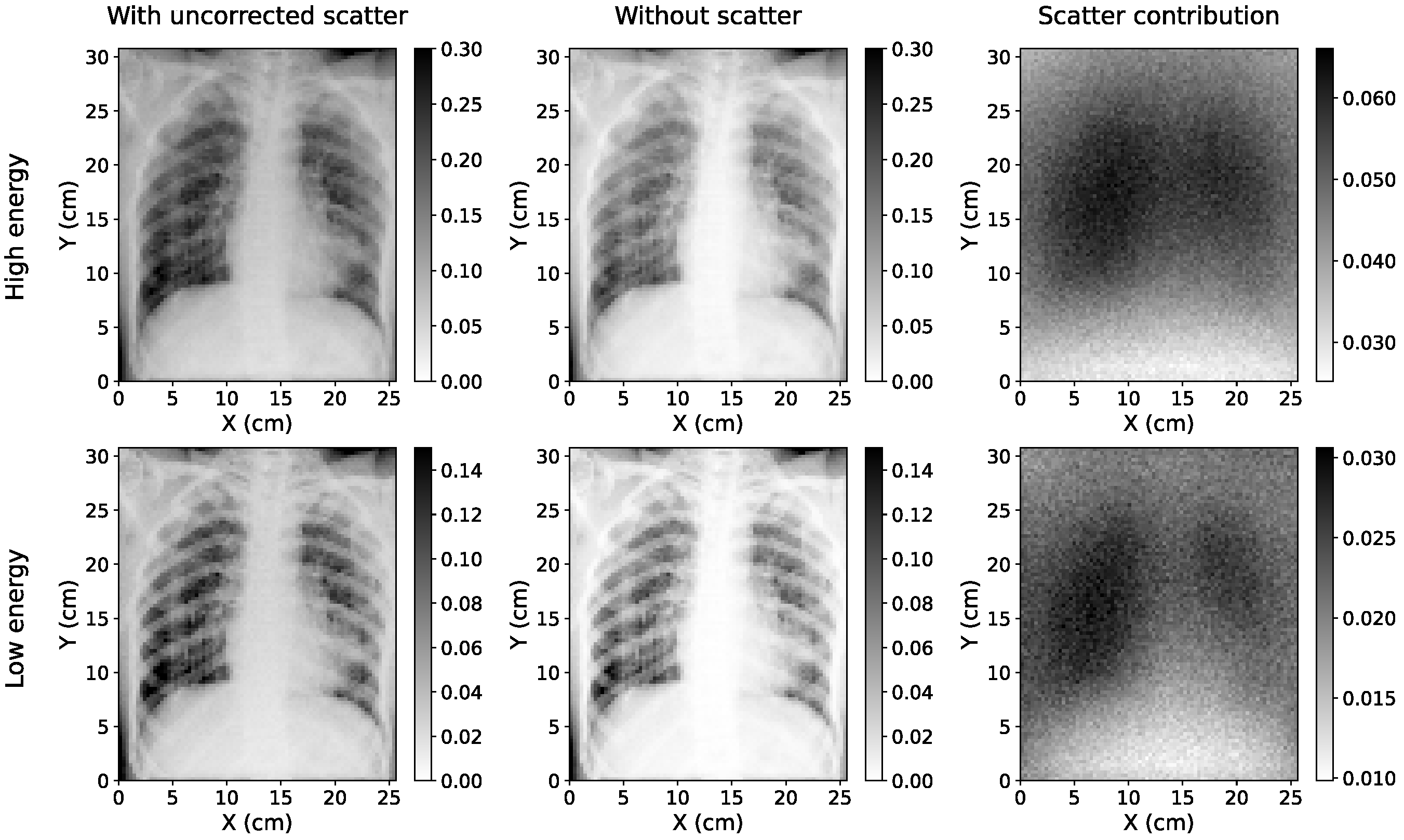
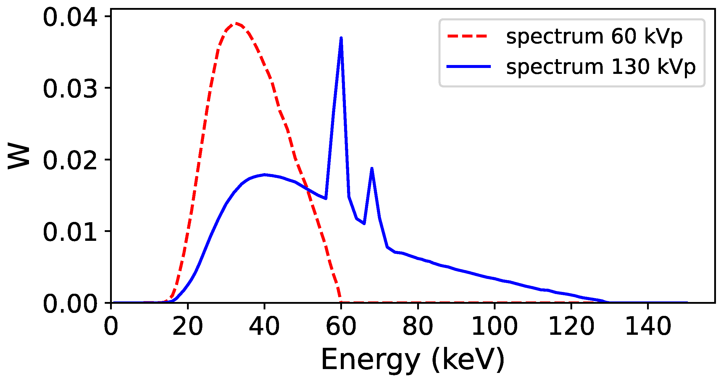
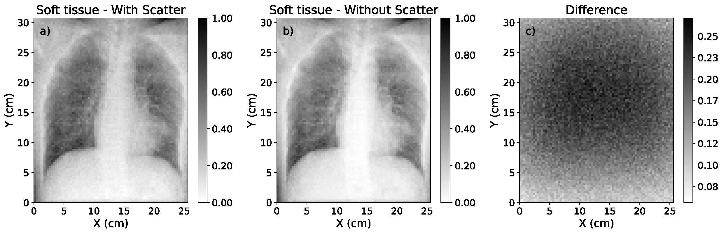
2.2. Monte Carlo Simulations to Generate Training and Validation Dataset

CT scans were represented in Hounsfield Units (HU). These values were converted to mass density, following work by Schneider et al. [42]. Additionally, the stretcher was removed by setting its HU values to be those of air. CXRs were acquired from these CT scans using a GPU-accelerated, ultrafast MC code developed in-house [43]. The code provided three projections for each patient: the scatter-free image (only primary photons), the scatter image (only scattered photons, considering both Rayleigh and Compton interactions), and the uncorrected-scatter image (both primary and secondary photon contributions). In all cases, the projections represented the photon energy that reaches the detector when there is an object (i.e., the patient) divided by the photon energy that would reach the detector in a simulation on air (see Figure 1). This way, all projections had values between 0 and 1. To be able to perform dual-energy training, images were acquired with two different X-ray energy spectra corresponding to 60 kVp (low energy) and 130 kVp (high energy) (Figure 2). The parameters of the simulation setup are gathered in

Table 1. Parameters of the MC simulation.

Parameter	Specification
Source-Detector Distance (cm)	180
X-ray Detector Size (cm)	$41\times 41$
X-ray Detector Resolution (pixel)	$2050\times 2050$

. A total of 5 × ${10}^9$ photons were simulated to obtain the three projections in the following way: the code-tracked photon path; if it had suffered any scatter interaction, its energy when arriving at the detector was used to form the scatter image; and if it had not undergone any interaction, the energy was saved to form the scatter-free image. After all photon histories were simulated, the uncorrected-scatter image was calculated as the sum of the scatter and scatter-free projections. Finally, a Gaussian filter was applied to the three images to smooth them. The simulation of the three projections for each energy spectra took about 10 min on a GeForce RTX 2080 Ti GPU.

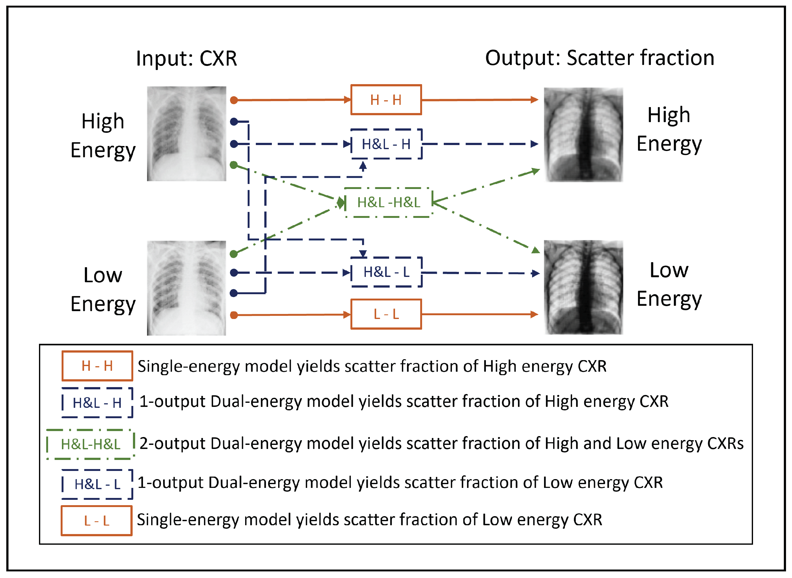
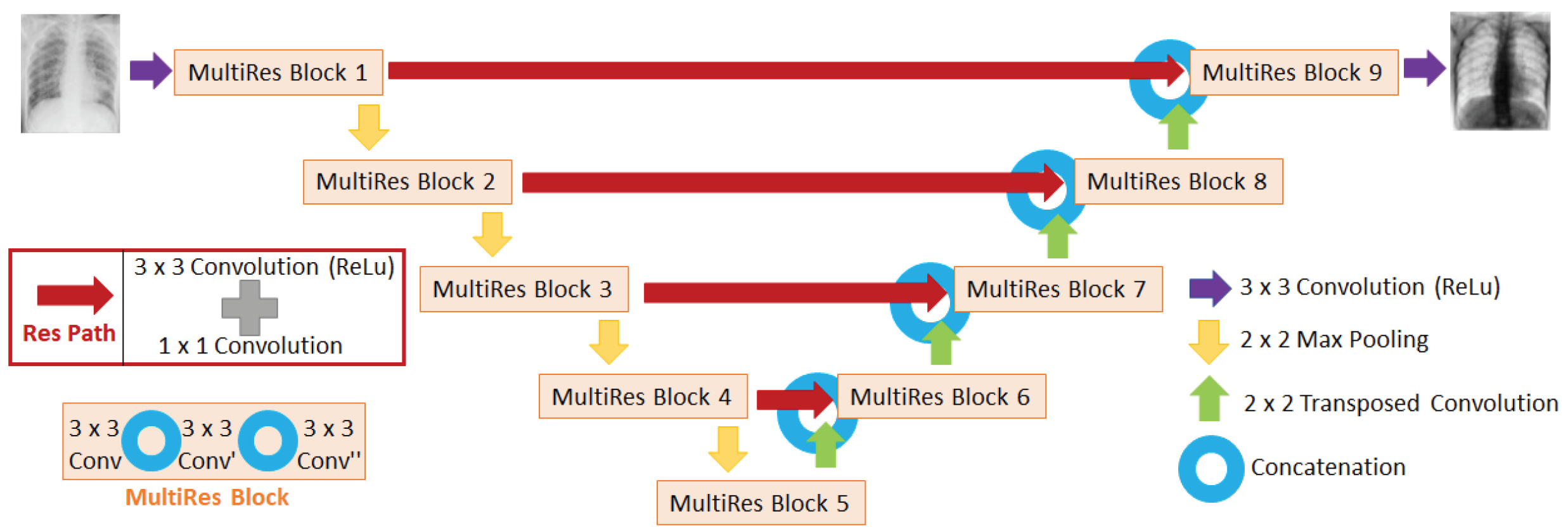
2.3. CNN Architecture

An enhanced U-Net-like architecture, named MultiResUNet, was used to train the NN models of scatter estimation. This evolution of the classical U-Net was first introduced by Ibtehaz and Rahman in 2019 [30]. It is based on an encoder–decoder model, which, in the standard U-Net architecture, takes the input image and performs four series of two $3\times 3$ convolution operations followed by a $2\times 2$ max pooling (encoder part), which is the size of the input image downsampled by a factor of 2 in each series. Then, another sequence of two $3\times 3$ convolutions joins the encoder and the decoder. The decoder first carries out a $2\times 2$ transposed convolution upsampling the feature map by a factor of 2, which is followed again by a series of two $3\times 3$ convolution operations. Finally, a $1\times 1$ convolution generates the output image [26]. Furthermore, U-Net architecture adds skip connections between the encoder and decoder, concatenating the output of the two convolution operations in the encoder and the output of the upsampling convolution in the decoder. These connections enable the NN to recover spatial data lost due to pooling procedures.

The MultiResUNet presents two main differences with respect to the standard U-Net. First, it substitutes the two consecutive $3\times 3$ convolution operations for three different $3\times 3$ convolutions, where the 2nd and the 3rd are intended to be approximately one $5\times 5$ and one $7\times 7$ procedure, respectively. Then, they are concatenated, and a $1\times 1$ convolutional layer (residual connection) is added. The result forms the so-called MultiRes block. Additionally, the NN does a batch normalization [46] to every convolutional layer. The second variation is related to the shortcut connections between the encoder and the decoder. A so-called residual path is computed with $3\times 3$ convolutions added to $1\times 1$ convolutional filters for residual connections. Then, the result is concatenated with the output of the transposed convolution in the decoder stage [30]. The scheme of the network is presented in Figure 3.

In this work, we used the MultiResUNet architecture with ReLU (Rectified Linear Unit) [47] as an activation function in every convolution output, including the last one, which provides the final output of the NN. The initial number of filters was set to 64, which increased by a factor of 2 in the downsampling steps, and afterward, it decreased by the same factor in the upsampling processes. In the single-energy model, there was one input and one output channel: the network took pairs of input–output images, with the input image being the uncorrected-scatter image and the output the fraction of the scatter image with respect to the uncorrected-scatter image (scatter ratio), both high-energy CXRs acquired with the 130 kVp energy spectrum. In the dual-energy workflow, we tested two different algorithms. On the one hand, a neural network with two input channels, corresponding to the uncorrected-scatter projections of low and high energy, and one output channel, representing the same as in the single-energy model (scatter ratio for the high energy case). From now on, we will refer to this model as a 1-output dual-energy model. On the other hand, we developed a 2-output dual-energy model, which had two input and two output channels, i.e., it estimated the scatter ratio of low and high-energy images at the same time. The single-energy model and the 1-output dual-energy model were also trained with low-energy images in order to obtain the corresponding scatter-corrected estimations. Figure 4 shows a scheme of input and output images corresponding to each of the described models. The use of the scatter ratio as the output of the NNs ensures that the image has values in the range 0–1, which is the standard range employed for the training of NNks and allows the use of ReLU as an activation function in the output layer.

The MultiResUNet was trained on Google Colab platform [48,49] on a Tesla T4 GPU, with 600 epochs using an Adam optimizer (with default parameters) [50], 10 steps per epoch, batch size of 24, and the mean squared error (MSE) as loss function. The original size of input and output images was equal to the resolution of the detector, i.e., $2050\times 2050$. To avoid memory problems, images were downsized to $128\times 128$ using bilinear interpolation. Additionally, images were cropped in the craneo–caudal direction to remove the edges (air voxels), so finally, the image size was $96\times 128$. We split the dataset into 70 training cases and 30 validation cases. As this number of cases is not enough to properly train a convolutional neural network, we performed data augmentation, including vertical and horizontal flips and zoom in up to 50%. These operations still provided realistic images.

The output of the network is multiplied by the uncorrected-scatter image, obtaining the scatter estimation. Then, the scatter estimation is subtracted from the input image, obtaining the estimated scatter-corrected image. The software takes 1.5 s to provide the scatter correction for each case, and multiple cases could be estimated simultaneously.

2.4. Evaluation of Scatter Estimation Models on Simulated CXRs

To assess the performance of the trained models, an additional test set of 22 CT images was taken from the same COVID-19 Lung CT Lesion database, and the three projections (scatter, scatter-free, and uncorrected scatter) were simulated as explained in Section 2.2. Four metrics were evaluated to quantify the accuracy of the scatter correction with the single and dual-energy NN models for the test set: the mean squared error (MSE), the mean absolute percentage error (MAPE), the structural similarity index (SSIM) and the relative error ($E_{rel}$), which are defined as:

$$MSE=\frac{1}{M\times N}\sum _{i=1}^M\sum _{j=1}^N{\parallel x_{i,j}-y_{i,j}\parallel }^2$$

(1)

$$MAPE=\frac{1}{M\times N}\sum _{i=1}^M\sum _{j=1}^N\left(\frac{|x_{i,j}-y_{i,j}|}{|x_{i,j}|}\right)\times 100$$

(2)

$$SSIM=\frac{1}{M\times N}\sum _{i=1}^M\sum _{j=1}^N\frac{\left(2{\mu }_x{\mu }_y+c_1\right)\left(2{\sigma }_{xy}+c_2\right)}{\left({\mu }_x^2+{\mu }_y^2+c_1\right)\left({\sigma }_x^2+{\sigma }_y^2+c_2\right)}\times 100$$

(3)

$$E_{rel}=\frac{1}{M\times N}\sum _{i=1}^M\sum _{j=1}^N\frac{|x_{i,j}-y_{i,j}|}{\left(x_{i,j}+y_{i,j}\right)}$$

(4)

where M and N are the number of pixels in the X and Y direction, and $x_{i,j}$ and $y_{i,j}$ are the values of ground truth and estimated images, respectively, for pixel $(i,j)$. In Equation (3), ${\mu }_x$ and ${\mu }_y$ are the average of $x_{i,j}$ and $y_{i,j}$; ${\sigma }_x$ and ${\sigma }_y$ are the standard deviations of $x_{i,j}$ and $y_{i,j}$; ${\sigma }_{xy}$ is the covariance of $x_{i,j}$ and $y_{i,j}$; $c_1={\left(K_{1}L\right)}^2$ and $c_2={\left(K_{2}L\right)}^2$, where L represents the range of pixel values and $K_1$ and $K_2$ are small positive constants that keep the denominator non-zero [51,52]. Metrics were applied to a region of interest (ROI) focused in the lungs.

The 22 CT test cases were simulated with 10 additional source-to-detector distances different from the one used to train the NN algorithms (SDD = 180 cm, see Table 1), from 100 to 200 cm. Then, the robustness of the models to variations in the SDD was evaluated with the above-mentioned metrics (Equations (1)–(4)).

To determine the gain when correcting scatter, a comparison of the contrast value in the lung between the COVID-19-affected region and the non-affected region on soft-tissue images was performed. Soft-tissue images were calculated by performing dual-energy subtraction, i.e., subtracting the low-energy CXR from the high-energy CXR. This operation was carried out for the uncorrected-scatter CXRs, the ground-truth scatter-corrected CXRs (Figure 5), and the estimated scatter-corrected CXRs with the three NNs. A mask of the COVID-19 region for each CT was found in the original database, so the COVID-19 region corresponding to the 2D projection was obtained with the MC simulation (Figure 6a). The lung mask was calculated with a U-Net CNN previously trained, with batch normalization, Adam optimizer, binary cross entropy as loss function, and sigmoid as output activation, and the mask of the healthy-lung region was obtained by subtracting the COVID-19 mask from the lung mask (Figure 6b).

The contrast metric is calculated as follows:

$$C=\frac{\frac{1}{F}{\sum }_{k=1}^{F}img\left(k\right)}{\frac{1}{G}{\sum }_{l=1}^{G}img\left(l\right)}$$

(5)

where F and G stand for the total number of pixels in the COVID-19 and the healthy-lung mask, respectively, and $img\left(k\right)$ and $img\left(l\right)$ represent the values of the given image $img$ in pixel k (COVID mask) or in pixel l (healthy-lung mask). To evaluate the contrast, each lung was considered to be a different case for patients who have both lungs affected, so there were 31 affected lungs in which the contrast was calculated. The accuracy of the NN models regarding the contrast was quantified by the relative difference with respect to the ground-truth value:

$$Di{f}_{rel}=100\times \frac{|C_{gt}-C_{NN}|}{C_{gt}}$$

(6)

where $C_{gt}$ is the contrast value in Equation (5) for the scatter-free ground-truth image (from MC simulation), and $C_{NN}$ is the contrast value for the NN estimation (single or dual-energy model) of the scatter correction.

Additionally, the percentage contrast improvement factor (PCIF) was computed as:

$$PCIF=100\times \frac{C_{corr}}{C_{uncorr}}-1$$

(7)

where $C_{corr}$ and $C_{uncorr}$ are the contrast values for the scatter-corrected and uncorrected image, respectively, calculated from Equation (5).

2.5. Evaluation of Scatter Correction on True CXRs

A set of 10 real CXRs acquired without an anti-scatter grid were taken from the MIMIC-CXR database [53,54] to test the single-energy model for high-energy CXRs on true data. To introduce these images as the input of the neural network, some operations must be performed. First, the CXR in Dicom format is loaded in a Python environment as a numpy array. Then, the edges of the images that do not contain information are cropped so that they are focused on the lung region. The original size of the CXRs selected from the database is $2544\times 3056$, so they are rescaled to $96\times 128$, as previously done with the simulated images (see Section 2.3). Finally, the values of the pixels in the true images must be converted to the same scale as in the training, simulated images. The values of the real CXR represent the logarithm of the initial beam intensity ($I_0$) divided by the intensity that arrives at the detector (I), while the values depicted in the training images are $I/I_0$, as explained in Section 2.2. So the transformation of pixel values is made following the Beer–Lambert law [55]: $I=I_0\times e^{-\mu \times x}$, where $\mu$ is the linear attenuation coefficient of the material, and x is the path length of the beam through the material; and then adjusting the scale so that the minimum and maximum values corresponding to bone and lungs are similar to the simulated images, as well as the ratio between them.

The output of the CNN, i.e., the scatter fraction, is multiplied by the downsized and scale-transformed CXR, yielding the estimation of the scatter contribution in low resolution. To obtain the final scatter-corrected CXR, the native resolution is recovered in the image of scatter by means of bilinear interpolation. Then, the high-resolution scatter image is subtracted from the high-resolution, scale-transformed CXR, giving the high-resolution scatter-corrected image.

The performance of the single-energy model on real data is quantitatively evaluated by means of the ratio between a region of the lung with and without ribs on it:

$$Ratio=\frac{\frac{1}{L}{\sum }_{m=1}^{L}img\left(m\right)}{\frac{1}{R}{\sum }_{n=1}^{R}img\left(n\right)}$$

(8)

where L and R stand for the total number of pixels of the rib-free lung region and the rib lung region, respectively, and $img\left(m\right)$ and $img\left(n\right)$ represent the values of the given image $img$ in pixel m (rib-free region) or in pixel n (rib lung region). The comparison of the ratio obtained in the original CXR (affected by the scatter) and in the estimation of the scatter-corrected image determines if the NN algorithm provides images with better contrast between different tissues.

3. Results

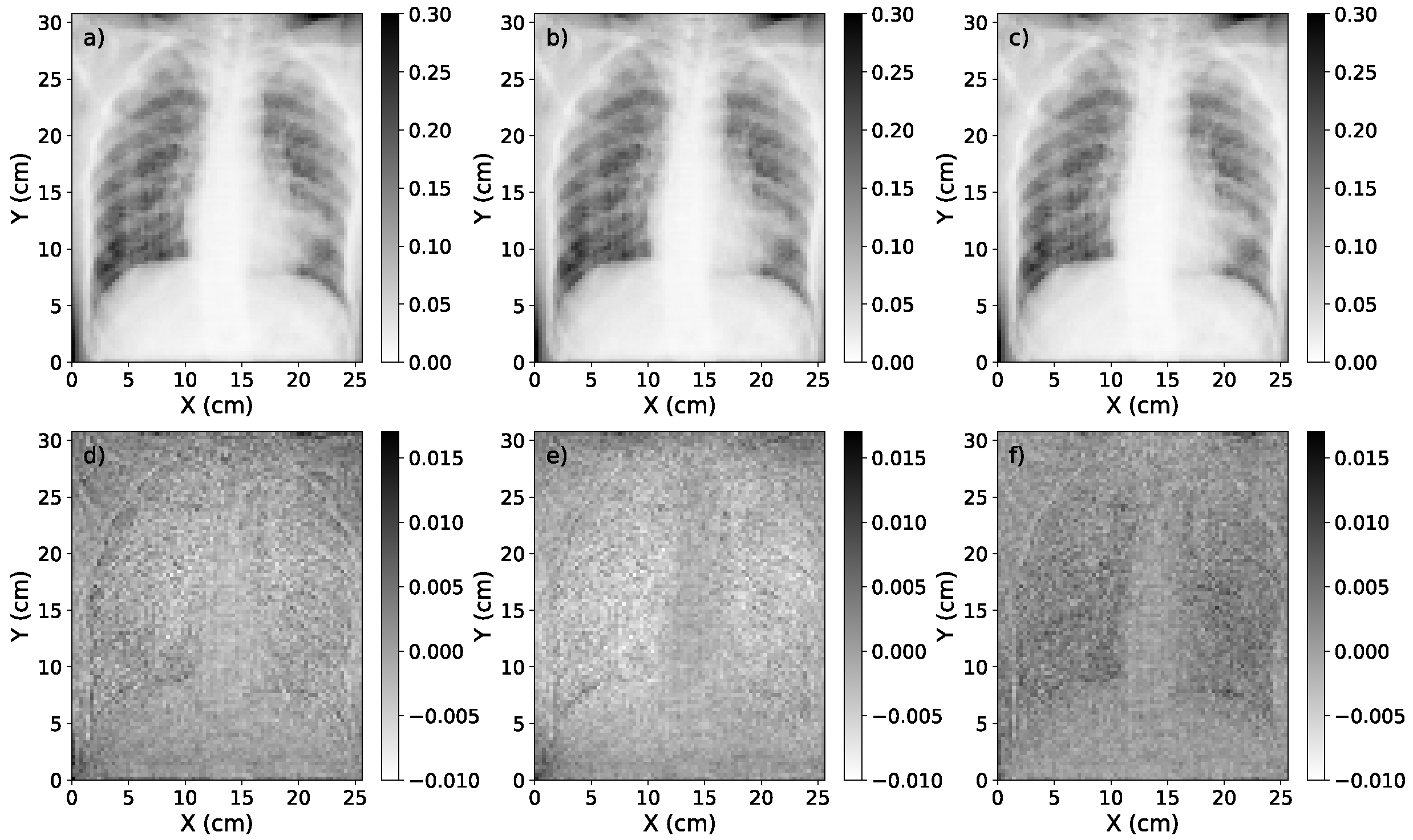
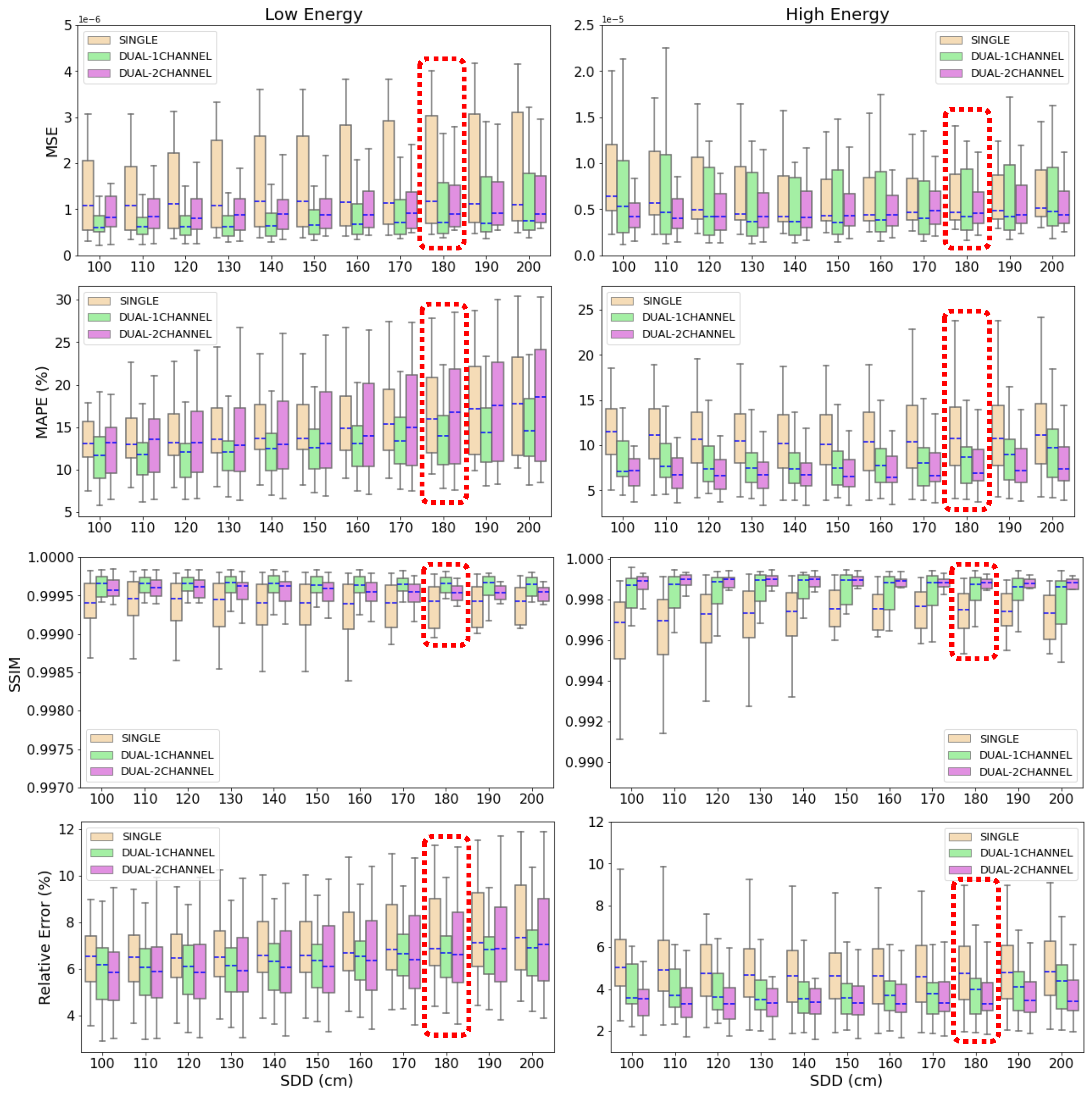
3.1. Accuracy of Scatter Correction on Simulated CXRs

An example of high-energy, scatter-corrected estimations of the single-energy model and the 1-output and 2-output dual-energy models are represented in Figure 7 for one of the test cases with SDD = 180 cm, as well as the differences between these estimations and the ground-truth scatter-corrected CXR, which is shown in Figure 1.

The values of MSE, MAPE, SSIM, and the relative error for the test cases with the original SDD and the ten additional variations are represented with a box plot (Figure 8). The results of the four metrics show that the scatter correction models provide an accurate estimation of the scatter correction for the original source-to-detector distance (SDD = 180 cm), highlighted with a red box. For the high-energy images, the average MSE is in the order of $7.3\times {10}^{-6}$, the MAPE indicates an average precision of 11.2%, 8.6%, and 7.6%, while the relative error presents mean values of 4.8%, 4.0%, and 3.6% for the single, 1-output dual-energy, and 2-output dual-energy models, respectively. Moreover, the average SSIM is 0.997 for the single-energy algorithm and 0.998 for both dual-energy NNs, which demonstrates that the outputs of the models have an elevated structural similarity to ground-truth images.

Regarding the scatter correction of low-energy images, the average MSE in the single-energy model is $2.2\times {10}^{-6}$, and $1.5\times {10}^{-6}$ for the two dual-energy networks. The MAPE is 17.1%, 14.0%, and 16.6% for the single-energy, 1-output dual-energy, and 2-output dual-energy models, respectively, while the relative error has average values of 7.3%, 6.7%, and 7.0%. The SSIM obtained in the three models is, on average, 0.999. Comparing the estimations for high-energy and low-energy images, it is observed that the MAPE and the relative error are higher in the models for low-energy scatter correction estimations, but good accuracy is still achieved.

In all graphics in Figure 8, it is observed that the mean values of the metrics evaluated over the test cases remain very similar for the different SDDs in relation to the original SDD with which the NNs were trained. In the high-energy estimations, the biggest increase among all the evaluated SDD for the MSE is 22.6% in the single-energy model, 15.5% in the 1-output dual-energy model, and 2.4% in the 2-output dual-energy model. In the MAPE, the greatest deviation from the mean value corresponding to SDD = 180 cm is 7.3%, 10.7%, and 3.9%, respectively. In the SSIM, the differences among the various SDD cases are barely relevant (0.06%, 0.04%, and 0.01%), while the major differences in the relative error are in the same order that the ones in the MAPE (7.6%, 8.6%, and 2.5% for single, 1-output and 2-output dual-energy algorithms, respectively). Similar results are obtained in the low-energy estimations: the major deviations are 3.1%, 14.0%, and 6.3% in MSE; 8.2%, 5.7%, and 9.0% in MAPE; and 4.1%, 4.5%, and 5.7%, for the single-energy, 1-output, and 2-output dual-energy models. Again, variations in SSIM are negligible. In all cases, the biggest deviations with respect to the original SDD are found either in SDD = 100 cm or SDD = 200 cm. Furthermore, graphics in Figure 8 show that the range of the maximum and minimum values of the metrics for the 22 test cases remains much the same in all SDDs in comparison with the original one.

Comparing the results of single- and dual-energy models, Figure 8 shows that the 2-output dual-energy algorithm yields higher accuracy in scatter correction considering the metrics of MAPE, SSIM, and relative error for high-energy CXRs, while in low-energy images, the best accuracy is obtained with the 1-output dual-energy algorithm. Taking as reference the case of SDD = 180 cm, in high-energy estimations, the average value of MAPE yielded by the 2-output dual-energy NN is 13% smaller than the one of the 1-output dual-energy model and 47% smaller with respect to the single-energy algorithm; the relative error is 33% and 11% better, respectively, while the SSIM is only 0.15% bigger in the 2-output dual-energy model than in the single-energy model, and 0.04% bigger with respect to the 1-output dual-energy NN, although a visual difference can be appreciated in the corresponding graphics. In the low-energy case, the 1-output dual-energy model outperforms the single-energy and the 2-output dual-energy algorithms in 22% and 19% in MAPE and a 9% and 4% in the relative error, respectively. The difference in the SSIM is minimal. Moreover, it is observed in Figure 8 that the model with the best accuracy in each case also has a lower standard deviation, represented by a smaller size of the box in the plot (green boxes in the metrics for low-energy estimations, corresponding to the 1-output dual-energy model, and violet boxes for high-energy estimations, corresponding to the 2-output dual-energy model). The relevance of the differences between the three algorithms will be further discussed in Section 4.

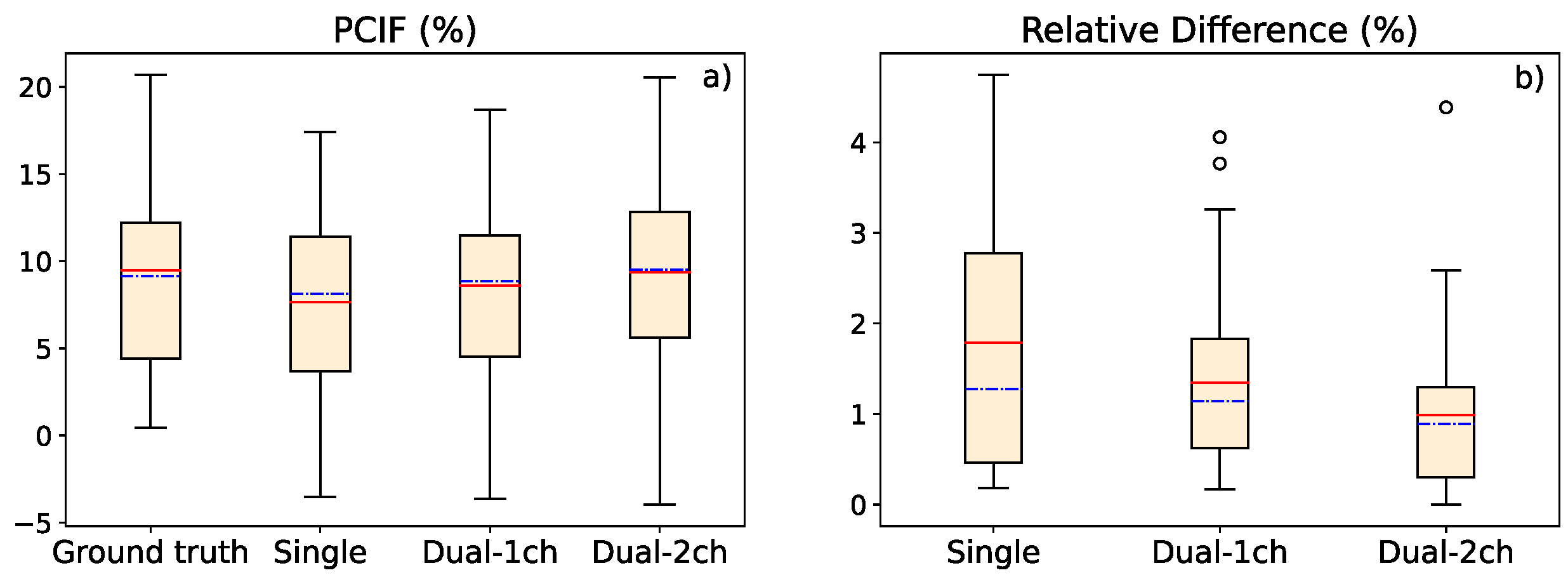
3.2. Study of Contrast Improvement after Scatter Correction

Table A1. Contrast value (Equation (5)) between the COVID-19-affected region and the healthy lung for the soft-tissue test images in the uncorrected image, the scatter-corrected ground-truth image and the scatter-corrected images estimated by the single-energy and dual-energy models. For patients with both lungs affected, each lung has been considered to be a different case.

Patient	Ground Truth Uncorrected Image	Ground Truth Scatter-Corrected Image	Scatter-Corrected with Single Energy	Scatter-Corrected with 1-Output Dual Energy	Scatter-Corrected with 2-Output Dual Energy
Case 1	1.216	1.385	1.352	1.374	1.380
Case 2	1.165	1.282	1.268	1.285	1.278
Case 3	1.032	1.101	1.072	1.080	1.095
Case 4	1.292	1.430	1.419	1.404	1.455
Case 5	1.187	1.299	1.289	1.293	1.299
Case 6	1.047	1.018	1.045	1.048	1.014
Case 7	1.147	1.239	1.235	1.231	1.255
Case 8	1.297	1.448	1.453	1.439	1.434
Case 9	1.096	1.301	1.244	1.252	1.284
Case 10	1.301	1.553	1.499	1.531	1.526
Case 11	1.154	1.201	1.195	1.198	1.190
Case 12	1.045	1.159	1.104	1.145	1.149
Case 13	0.795	0.645	0.648	0.684	0.627
Case 14	1.209	1.454	1.403	1.434	1.436
Case 15	1.305	1.575	1.532	1.549	1.573
Case 16	1.128	1.176	1.170	1.198	1.184
Case 17	0.960	0.931	0.922	0.953	0.928
Case 18	1.104	1.202	1.173	1.205	1.213
Case 19	1.037	1.035	1.052	1.045	1.040
Case 20	0.879	0.890	0.864	0.861	0.913
Case 21	1.110	1.115	1.113	1.103	1.114
Case 22	1.021	1.056	1.054	1.063	1.058
Case 23	0.945	0.987	0.967	0.972	1.001
Case 24	1.098	1.165	1.148	1.163	1.162
Case 25	1.209	1.324	1.327	1.333	1.325
Case 26	1.183	1.279	1.293	1.287	1.291
Case 27	0.962	0.886	0.898	0.899	0.851
Case 28	0.841	0.719	0.719	0.723	0.717
Case 29	0.872	0.816	0.795	0.817	0.791
Case 30	0.908	0.912	0.876	0.875	0.872
Case 31	1.316	1.532	1.529	1.562	1.544

in the Appendix A shows the contrast between the region affected by COVID-19 and the healthy-lung area in the soft-tissue DES images. In 24 out of the 31 cases, the scatter-corrected ground-truth DES has higher contrast than the uncorrected DES, meaning that the scatter correction will help to better identify the lesion. In these cases, the average contrast improvement in the area of the lesion is 9.5%, with a maximum value of 20.7% (see Figure 9a).

It can be observed in Figure 9a that the three scatter correction methods proposed in this work are able to provide a very accurate percentage contrast improvement factor if results are compared with the ground truth (taken from the MC simulation). The single-energy model yields an average contrast improvement of 7.7%, with a maximum of 17.4%, while the 1-output dual-energy model gives an average PCIF of 8.6% and a maximum of 18.7%, and the 2-output dual-energy NN the average PCIF is 9.4% and its maximum value is 20.5%. These numbers again indicate that the 2-output dual-energy model has the best performance, although the difference with the other two algorithms is small, and the three models are acceptable. Figure 9b represents the relative difference between the ground-truth contrast value and the contrast value estimated by the three NN models, and it reinforces what was explained for Figure 9a: the relative difference is smaller for the 2-output dual-energy model, being in the range of 0–4.4%, with a mean value of 1.0%. For its part, the relative difference for the single-energy results varies from 0.2% to 4.7%, and the average relative difference is 1.8%; while for the 1-output dual-energy model, the relative difference is between 0.2% and 4.1%, being on average 1.3%. All these results point out that the contrast improvement factor associated with the scatter correction is estimated with very high precision by the three deep-learning-based models.

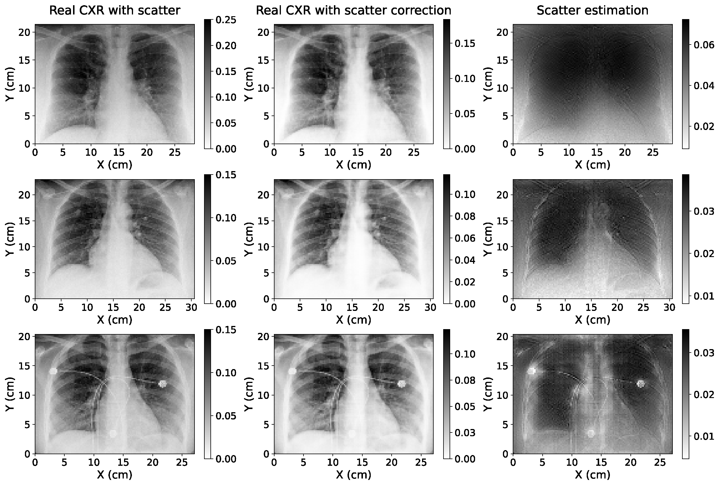
3.3. Study of Scatter Correction on True CXRs

Figure 10 shows the estimations of the scatter contribution and the scatter-corrected images of three real CXRs after applying the single-energy algorithm, along with the corresponding image used as input of the network, i.e., the original CXR (with scatter) with pixel values transform as explained in Section 2.5. In all cases, the NN model is able to make a proper estimation of the scattered-rays image and thus provide a scatter-corrected image comparable to what was expected according to the ground-truth simulation and the corresponding estimations (see Figure 1 and Figure 7), both qualitative and quantitatively.

Table 2. Ratio between a region of the lung with and without rib in the original, real CXRs and in the scatter-corrected CXRs yielded by the single-energy algorithm for the 10 CXRs taken as test set (listed as C1–C10), and the resulting average value.

	C1	C2	C3	C4	C5	C6	C7	C8	C9	C10	Avg
Original	2.71	1.66	1.36	1.11	1.35	1.16	1.71	1.47	1.28	1.59	1.54
Scatter-corrected	3.80	2.02	1.54	1.17	1.49	1.23	2.14	1.68	1.41	1.64	1.81

shows the ratio between a region of the lung with and without rib in the CXR before and after the single-energy scatter correction algorithm is applied to the 10 test images. The ratio increases in every sample when the NN model of scatter correction is implemented, with an average rise of 15.0% for the selected cohort, with a maximum increase of 40.2%.

4. Discussion

In this work, we have implemented and evaluated the performance of three deep-learning models that estimate and correct the scatter in CXRs. One model is based on standard single-energy acquisitions, while the other two models assume that two CXRs with different energies (dual energy) were acquired per patient. The impact of varying the distance of the X-ray source on the accuracy of the scatter correction with these methods was studied.

Results in Figure 8 demonstrate that the three deep-learning-based models are able to accurately estimate and correct scatter contribution to simulated CXRs. Moreover, the three algorithms keep their accuracy on scatter correction when the source-to-detector distance (SDD) varies in a range of 100 cm from the SDD used to train the neural networks. Thus, the results prove that the models are robust to variations on the setup parameters, such as air gap or SDD, and their application is not limited to a specific configuration.

The highest decrease in accuracy is found in SDD = 100 cm and SDD = 200 cm (the neural networks were trained with SDD = 180 cm). For SDD = 100 cm, this result could be expected since it is the case with the largest distance with respect to the reference SDD. The fact that less accurate metrics are obtained for SDD = 200 cm, which is the second closest distance to the one of reference, indicates that the models are more accurate if the images are well focused on the lungs and the air-background areas are reduced or cropped. In this case, the lungs become smaller in the image as the SDD increases, which explains the loss of accuracy.

According to the mean values of MAPE and relative error shown in Section 3.1, the results obtained with the dual-energy NN models are more accurate than the ones provided by the single-energy model. In the estimations of the scatter-corrected high-energy CXRs, the p-value between the metrics yielded by the 2-output dual-energy and the single-energy models is $p=4.2\times {10}^{-13}$ for the MAPE, and $p=0.01$ for the relative error, i.e., in both metrics the p-value is below the classic threshold of 0.05 [56,57], indicating that the difference is statistically significant. In the low-energy estimations, the p-value between the 1-output dual-energy and the single-energy algorithms is $p=0.05$ for the MAPE and $p=0.28$ for the relative error, so the difference is significant only in the first metric. As explained in Section 3.1, the difference in the SSIM is minor. Regarding the MSE, there is not a substantial difference between the three models due to the fact that this is the metric employed as a loss function in the training of the algorithms, so it is minimized in both cases. In the comparison between the two proposed models of scatter correction, it is also observed in Figure 8 that there is less deviation in the values of MAPE and relative error applying the dual-energy model. In the high-energy case, the standard deviation in MAPE is 4.9%, 3.4%, and 2.6% for single-energy, 1-output, and 2-output dual-energy models, respectively, and the deviation in the relative error is 1.8% for the single-energy network, 1.4% for the 1-output dual-energy algorithm, and 1.1% for the 2-output-dual-energy algorithm. In the low-energy case, the standard deviation in MAPE is 6.0%, 4.1%, and 6.3% for the single-energy, 1-output, and 2-output dual-energy models, and the corresponding values in the relative error are 2.0%, 1.5%, and 2.2%, respectively. All these results point to the superior performance of the dual-energy models for scatter correction of CXRs, being more accurate in the 1-output model for low-energy acquisitions and the 2-output model for high-energy images.

The application of the single-energy model to real CXRs acquired without an anti-scatter grid suggests that the algorithm can be easily adapted to be used with true data acquired with different setups since, in this case, the information of the parameters with which the projections were taken was not available in the anonymized Dicom headers used. Furthermore, the accuracy of the model applied to these images could not be quantitatively determined as there was no access to ground-truth, scatter-free CXRs. However, Figure 10 shows that the estimations are robust, even for radiography with artifacts such as wires, as it happens in the third case of this Figure. This is a key aspect, as the application of these models can be especially useful for critically ill patients with whom it is more difficult to utilize an anti-scatter grid (as explained in Section 1). In addition, the values of the ratio between the regions of the lung with and without ribs (Table 2) point out that the scatter correction improves the contrast between different tissues.

The two dual-energy models could not be verified against real data since we currently do not have access to CXRs acquired with two different X-ray kilovoltages. Nevertheless, it is expected that good estimations of scatter-corrected images can be obtained in actual images, in light of the results shown in Section 3.1 and Section 3.3. Moreover, the superior accuracy shown by the 1-output and 2-output dual-energy models when evaluating the MAPE and the relative error, which has been previously discussed in this Section and in Section 3.1, would be worth studying in future research with real CXRs acquired without an anti-scatter grid with two different energy spectra. This way, it could be determined if dual-energy approaches truly provide better scatter correction, and the gain in DES images after scatter correction could also be tested.

Lee and Lee [9] performed a similar study on CXR scatter correction using CNNs and Monte Carlo simulations to generate training cases. They evaluated the SSIM, among other metrics, obtaining an average value of 0.992. This is in the same order as the 0.997 value yielded by the models herein proposed, with ours 0.5% better. As stated by these authors [9], the application of deep learning to scatter correction of CXR has only recently started, so there are not many studies with which results can be compared. Some literature on scatter correction (or estimation) on cone-beam CT images can be found. Roser et al. [13] presented a scatter estimation method based on a deep-learning approach, helped by bivariate B-spline approximation. For thorax CT, the MAPE ranges approximately from 3% to 20% for the five-fold cross-validations, while our models obtain average values of 11.2% and 8.6%. Additionally, the SSIM for the thorax CT study is between 0.96 and 0.99. Although CT and CXR have some obvious differences, and they are not exactly comparable, it can be noticed that our models present a similar precision.

The models displayed in this paper still have some limitations that would need further study. First, we uniquely employed simulated images for the training and validation, as well as for the test cases in Section 3.1. Thus, when these NNs are applied to real CXRs, the accuracy of the scatter correction depends on the precision of the Monte Carlo codes. Despite the fact that MC simulations are the gold standard in the field and provide very realistic images, some works for scatter estimation in CT showed that the accuracy of deep-learning models could decrease when applying to real images NNs trained only with simulated images [19]. For CXRs, more studies are needed to determine the accuracy of neural networks in this situation. Since having a sufficient amount of cases to train only with real data is complex in this field, it would be convenient to obtain images that are as realistic as possible. For this purpose, if at least some real cases are available, the use of generative adversarial networks (GANs) [58] in combination with MC simulations could achieve this goal and thus improve the accuracy of the models applied to real data.

It is important to note that the input–output pairs of images of the neural network are exclusively uncorrected-scatter–scatter ratio images. That is to say, the models are not trained to distinguish if the input image is affected by scatter, so if a scatter-free projection is given to the network, it will still yield some scatter estimation. The subtraction of this estimated image from a scatter-free input image would entail some loss of information in the final result. Therefore, these models cannot be applied to acquisitions taken with an anti-scatter grid or any other scatter suppression technique, and neither can be used to check the effectiveness in scatter removal of those hardware-based scatter suppression methods. A neural network that identifies if the input image is affected by scattered rays is currently being implemented, but it is beyond the scope of this work.

As explained in Section 2.3, an ROI focus primarily on the lungs was selected in the training, validation, and test images (see Figure 1). This way, the edges of the images that could cause the appearance of artifacts in the scatter estimation and the scatter-corrected images are removed. This allows us to obtain very accurate results, but it must be taken into account before putting the models into practice. An input image with a large number of empty regions could compromise the robustness of the models, just as suggested by the results obtained for images simulated SDD = 200 cm.

Although the number of training and validation cases might seem small, the variety in the patient sizes within the dataset (explained in Section 2.1), along with the data augmentation described in Section 2.3, guarantees the accuracy of the models for images with different amounts of scatter ratio.

The fact that the contrast C (Section 3.2) and the ratio between lung regions with and without rib (Section 3.3) improve after the application of the presented deep-learning models implies that the detection and diagnosis of COVID-19 will be enhanced after scatter correction since it will help physicians to better differentiate infected areas of the lung. This deep-learning-based tool can be easily implemented in the software used by physicians so they can obtain scatter-corrected chest X-rays in a couple of seconds.

In this work, we focused on COVID-19 since a large number of databases related to this disease have been gathered in recent years as a consequence of the worldwide pandemic. However, the same analysis could be performed for any other pulmonary affection, such as pneumonia, tumors, atelectasis, and pneumothorax. It is highly expected that the scatter correction will also entail a contrast improvement in areas affected by any of these lesions and, therefore, facilitate its identification. Furthermore, similar deep-learning-based models could be applied to other types of medical imaging modalities affected by background noise, in which contrast can be improved, therefore enhancing image quality and diagnostic accuracy.

It should be taken into account that an overestimation in the contrast value could result in a loss of important information for medical diagnosis in the final scatter-corrected image. Results in Table A1 show that the contrast is overestimated in 7 out of 31 cases in the single-energy model, in 14 cases in the 1-output dual-energy model, and 11 cases in the 2-output dual-energy model. Nevertheless, the difference with the ground-truth value is, on average, just 1.11% for the single-energy method, 1.48% for the 1-output dual-energy network, and 1.01% for the 2-output dual-energy model. Thus, the overestimation is not significant and will not jeopardize the image information.

This work has been focused on the dataset generation, comparison of different inputs and outputs, and evaluation of the performance from the point of view of robustness. We have not performed extensive optimization of the hyperparameters of the NNs as we have used hyperparameters similar to the ones of the reference work of the MultiResUNet architecture [30].

5. Conclusions

In this work, we presented three deep-learning-based methods to estimate the scatter contribution in CXRs and obtain scatter-corrected projections: A single-energy model, with one input and one output image; a 1-output dual-energy model, in which a projection acquired with a different energy spectrum is set as an additional input channel, but the output has only one channel; and a 2-output dual-energy model, in which the scatter estimation is provided for the two energies introduced in the two input channels. The three models were robust to variations in the SDD, obtaining a high precision for distances in a range between 100 and 200 cm and proving that a similar accuracy with respect to images with the original SDD of the training data (SDD = 180 cm) can be maintained. Moreover, the contrast values between the lung region affected by COVID-19 and the healthy region in soft-tissue images (obtained by means of dual-energy subtraction) demonstrated that scatter correction in CXRs provides better contrast to the area of the lesion, yielding a PCIF of up to 20.5%.

In both studies (accuracy in scatter correction for several SDD and contrast value in COVID-19 region), the dual-energy algorithms provide results with better accuracy. The analysis of the p-value demonstrates that the difference in accuracy between the single-energy and dual-energy models can be statistically significant, especially in the scatter-corrected estimations of high-energy CXRs with the 2-output method. The single-energy algorithm is accurate enough for scatter correction of CXRs, so it might not be worth acquiring an extra CXR just for this purpose. However, dual-energy models are proven to be a useful tool for scatter correction on soft-tissue DES CXRs.

The single-energy model was tested with a cohort of real CXRs acquired without an anti-scatter grid, yielding robust, qualitative estimations of the scatter correction, even for images with artifacts. Further studies with real phantoms and patients should be performed to quantitatively determine the precision of the three models with real data and analyze whether the difference between the performance of the single- and dual-energy algorithms is relevant.

References

1. Candemir, S.; Antani, S. A review on lung boundary detection in chest x-rays. Int. J. Comput. Assist. Radiol. Surg. 2019, 14, 563–576. [Google Scholar] [CrossRef] [PubMed]
2. Gange, C.P.; Pahade, J.K.; Cortopassi, I.; Bader, A.S.; Bokhari, J.; Hoerner, M.; Thomas, K.M.; Rubinowitz, A.N. Social distancing with portable chest radiographs during the COVID-19 pandemic: Assessment of radiograph technique and image quality obtained at 6 feet and through glass. Radiol. Cardiothorac. Imaging 2020, 2, e200420. [Google Scholar] [CrossRef] [PubMed]
3. Çallı, E.; Sogancioglu, E.; van Ginneken, B.; van Leeuwen, K.G.; Murphy, K. Deep learning for chest X-ray analysis: A survey. Med. Image Anal. 2021, 72, 102125. [Google Scholar] [CrossRef] [PubMed]
4. Raoof, S.; Feigin, D.; Sung, A.; Raoof, S.; Irugulpati, L.; Rosenow, E.C., III. Interpretation of plain chest roentgenogram. Chest 2012, 141, 545–558. [Google Scholar] [CrossRef] [PubMed]
5. Shaw, D.; Crawshaw, I.; Rimmer, S. Effects of tube potential and scatter rejection on image quality and effective dose in digital chest X-ray examination: An anthropomorphic phantom study. Radiography 2013, 19, 321–325. [Google Scholar] [CrossRef]
6. Jones, J.; Murphy, A.; Bell, D. Chest Radiograph. Available online: https://radiopaedia.org/articles/chest-radiograph?lang=us (accessed on 7 February 2023).
7. Mentrup, D.; Neitzel, U.; Jockel, S.; Maack, H.; Menser, B. Grid-Like Contrast Enhancement for Bedside Chest Radiographs Acquired without Anti-Scatter Grid; Philips SkyFlow: Amsterdam, The Netherlands, 2014. [Google Scholar]
8. Seibert, J.A.; Boone, J.M. X-ray imaging physics for nuclear medicine technologists. Part 2: X-ray interactions and image formation. J. Nucl. Med. Technol. 2005, 33, 3–18. [Google Scholar] [PubMed]
9. Lee, H.; Lee, J. A deep learning-based scatter correction of simulated X-ray images. Electronics 2019, 8, 944. [Google Scholar] [CrossRef]
10. Liu, X.; Shaw, C.C.; Lai, C.J.; Wang, T. Comparison of scatter rejection and low-contrast performance of scan equalization digital radiography (SEDR), slot-scan digital radiography, and full-field digital radiography systems for chest phantom imaging. Med. Phys. 2011, 38, 23–33. [Google Scholar] [CrossRef]
11. Rührnschopf, E.P.; Klingenbeck, K. A general framework and review of scatter correction methods in X-ray cone-beam computerized tomography. Part 1: Scatter compensation approaches. Med. Phys. 2011, 38, 4296–4311. [Google Scholar] [CrossRef]
12. Chan, H.P.; Lam, K.L.; Wu, Y. Studies of performance of antiscatter grids in digital radiography: Effect on signal-to-noise ratio. Med. Phys. 1990, 17, 655–664. [Google Scholar] [CrossRef]
13. Roser, P.; Birkhold, A.; Preuhs, A.; Syben, C.; Felsner, L.; Hoppe, E.; Strobel, N.; Kowarschik, M.; Fahrig, R.; Maier, A. X-ray scatter estimation using deep splines. IEEE Trans. Med. Imaging 2021, 40, 2272–2283. [Google Scholar] [CrossRef] [PubMed]
14. Gauntt, D.M.; Barnes, G.T. Grid line artifact formation: A comprehensive theory. Med. Phys. 2006, 33, 1668–1677. [Google Scholar] [CrossRef] [PubMed]
15. Bernhardt, T.; Rapp-Bernhardt, U.; Hausmann, T.; Reichel, G.; Krause, U.; Doehring, W. Digital selenium radiography: Anti-scatter grid for chest radiography in a clinical study. Br. J. Radiol. 2000, 73, 963–968. [Google Scholar] [CrossRef] [PubMed]
16. Roberts, J.; Evans, S.; Rees, M. Optimisation of imaging technique used in direct digital radiography. J. Radiol. Prot. 2006, 26, 287. [Google Scholar] [CrossRef] [PubMed]
17. Moore, C.; Avery, G.; Balcam, S.; Needler, L.; Swift, A.; Beavis, A.; Saunderson, J. Use of a digitally reconstructed radiograph-based computer simulation for the optimisation of chest radiographic techniques for computed radiography imaging systems. Br. J. Radiol. 2012, 85, e630–e639. [Google Scholar] [CrossRef] [PubMed]
18. Lifton, J.; Malcolm, A.; McBride, J. An experimental study on the influence of scatter and beam hardening in X-ray CT for dimensional metrology. Meas. Sci. Technol. 2015, 27, 015007. [Google Scholar] [CrossRef]
19. Maier, J.; Sawall, S.; Knaup, M.; Kachelrieß, M. Deep scatter estimation (DSE): Accurate real-time scatter estimation for X-ray CT using a deep convolutional neural network. J. Nondestruct. Eval. 2018, 37, 1–9. [Google Scholar] [CrossRef]
20. Swindell, W.; Evans, P.M. Scattered radiation in portal images: A Monte Carlo simulation and a simple physical model. Med. Phys. 1996, 23, 63–73. [Google Scholar] [CrossRef]
21. Bhatia, N.; Tisseur, D.; Buyens, F.; Létang, J.M. Scattering correction using continuously thickness-adapted kernels. NDT Int. 2016, 78, 52–60. [Google Scholar] [CrossRef]
22. Codella, N.C.; Gutman, D.; Celebi, M.E.; Helba, B.; Marchetti, M.A.; Dusza, S.W.; Kalloo, A.; Liopyris, K.; Mishra, N.; Kittler, H.; et al. Skin lesion analysis toward melanoma detection: A challenge at the 2017 international symposium on biomedical imaging (ISBI), hosted by the international skin imaging collaboration (ISIC). In Proceedings of the 2018 IEEE 15th International Symposium on Biomedical Imaging (ISBI 2018), Washington, DC, USA, 4 April 2018. [Google Scholar]
23. Sermanet, P.; Eigen, D.; Zhang, X.; Mathieu, M.; Fergus, R.; LeCun, Y. Overfeat: Integrated recognition, localization and detection using convolutional networks. arXiv 2013, arXiv:1312.6229. [Google Scholar]
24. Rouhi, R.; Jafari, M.; Kasaei, S.; Keshavarzian, P. Benign and malignant breast tumors classification based on region growing and CNN segmentation. Expert Syst. Appl. 2015, 42, 990–1002. [Google Scholar] [CrossRef]
25. Krizhevsky, A.; Sutskever, I.; Hinton, G.E. Imagenet classification with deep convolutional neural networks. Commun. ACM 2017, 60, 84–90. [Google Scholar] [CrossRef]
26. Ronneberger, O.; Fischer, P.; Brox, T. U-net: Convolutional networks for biomedical image segmentation. In Proceedings of the Medical Image Computing and Computer-Assisted Intervention—MICCAI 2015: 18th International Conference, Munich, Germany, 5 October 2015. [Google Scholar]
27. Siddique, N.; Paheding, S.; Elkin, C.P.; Devabhaktuni, V. U-net and its variants for medical image segmentation: A review of theory and applications. IEEE Access 2021, 9, 82031–82057. [Google Scholar] [CrossRef]
28. Moon, J.H.; Lee, H.; Shin, W.; Kim, Y.H.; Choi, E. Multi-modal understanding and generation for medical images and text via vision-language pre-training. IEEE J. Biomed. Health Inform. 2022, 26, 6070–6080. [Google Scholar] [CrossRef]
29. Liu, C.; Cheng, S.; Chen, C.; Qiao, M.; Zhang, W.; Shah, A.; Bai, W.; Arcucci, R. M-FLAG: Medical vision-language pre-training with frozen language models and latent space geometry optimization. In Proceedings of the Medical Image Computing and Computer-Assisted Intervention—MICCAI 2023: 26th International Conference, Vancouver, BC, Canada, 8 October 2023. [Google Scholar]
30. Ibtehaz, N.; Rahman, M.S. MultiResUNet: Rethinking the U-Net architecture for multimodal biomedical image segmentation. Neural Netw. 2020, 121, 74–87. [Google Scholar] [CrossRef] [PubMed]
31. Alvarez, R.E.; Macovski, A. Energy-selective reconstructions in X-ray computerised tomography. Phys. Med. Biol. 1976, 21, 733. [Google Scholar] [CrossRef]
32. Sellerer, T.; Mechlem, K.; Tang, R.; Taphorn, K.A.; Pfeiffer, F.; Herzen, J. Dual-energy X-ray dark-field material decomposition. IEEE Trans. Med. Imaging 2020, 40, 974–985. [Google Scholar] [CrossRef] [PubMed]
33. Fredenberg, E. Spectral and dual-energy X-ray imaging for medical applications. Nucl. Instrum. Methods Phys. Res. A 2018, 878, 74–87. [Google Scholar] [CrossRef]
34. Martz, H.E.; Glenn, S.M. Dual-Energy X-ray Radiography and Computed Tomography; Technical Report; Lawrence Livermore National Lab (LLNL): Livermore, CA, USA, 2019.
35. Marin, D.; Boll, D.T.; Mileto, A.; Nelson, R.C. State of the art: Dual-energy CT of the abdomen. Radiology 2014, 271, 327–342. [Google Scholar] [CrossRef]
36. Manji, F.; Wang, J.; Norman, G.; Wang, Z.; Koff, D. Comparison of dual energy subtraction chest radiography and traditional chest X-rays in the detection of pulmonary nodules. Quant. Imaging Med. Surg. 2016, 6, 1. [Google Scholar]
37. Vock, P.; Szucs-Farkas, Z. Dual energy subtraction: Principles and clinical applications. Eur. J. Radiol. 2009, 72, 231–237. [Google Scholar] [CrossRef] [PubMed]
38. Yang, F.; Weng, X.; Miao, Y.; Wu, Y.; Xie, H.; Lei, P. Deep learning approach for automatic segmentation of ulna and radius in dual-energy X-ray imaging. Insights Imaging 2021, 12, 191. [Google Scholar] [CrossRef]
39. Luo, R.; Ge, Y.; Hu, Z.; Liang, D.; Li, Z.C. DeepPhase: Learning phase contrast signal from dual energy X-ray absorption images. Displays 2021, 69, 102027. [Google Scholar] [CrossRef]
40. Lee, D.; Kim, H.; Choi, B.; Kim, H.J. Development of a deep neural network for generating synthetic dual-energy chest X-ray images with single X-ray exposure. Phys. Med. Biol. 2019, 64, 115017. [Google Scholar] [CrossRef] [PubMed]
41. Roth, H.R.; Xu, Z.; Tor-Díez, C.; Jacob, R.S.; Zember, J.; Molto, J.; Li, W.; Xu, S.; Turkbey, B.; Turkbey, E.; et al. Rapid artificial intelligence solutions in a pandemic—The COVID-19-20 lung CT lesion segmentation challenge. Med. Image Anal. 2022, 82, 102605. [Google Scholar] [CrossRef] [PubMed]
42. Schneider, U.; Pedroni, E.; Lomax, A. The calibration of CT Hounsfield units for radiotherapy treatment planning. Phys. Med. Biol. 1996, 41, 111. [Google Scholar] [CrossRef] [PubMed]
43. Ibáñez, P.; Villa-Abaunza, A.; Vidal, M.; Guerra, P.; Graullera, S.; Illana, C.; Udías, J.M. XIORT-MC: A real-time MC-based dose computation tool for low-energy X-rays intraoperative radiation therapy. Med. Phys. 2021, 48, 8089–8106. [Google Scholar] [CrossRef] [PubMed]
44. Punnoose, J.; Xu, J.; Sisniega, A.; Zbijewski, W.; Siewerdsen, J. Technical note: Spektr 3.0—A computational tool for x-ray spectrum. Med. Phys. 2016, 43, 4711–4717. [Google Scholar] [CrossRef]
45. Sisniega, A.; Desco, M.; Vaquero, J. Modification of the tasmip X-ray spectral model for the simulation of microfocus X-ray sources. Med. Phys. 2014, 41, 011902. [Google Scholar] [CrossRef]
46. Ioffe, S.; Szegedy, C. Batch normalization: Accelerating deep network training by reducing internal covariate shift. In Proceedings of the International Conference on Machine Learning, Lille, France, 6 July 2015. [Google Scholar]
47. Hara, K.; Saito, D.; Shouno, H. Analysis of function of rectified linear unit used in deep learning. In Proceedings of the 2015 International Joint Conference on Neural Networks (IJCNN), Killarney, Ireland, 12 July 2015. [Google Scholar]
48. Carneiro, T.; Da Nóbrega, R.V.M.; Nepomuceno, T.; Bian, G.B.; De Albuquerque, V.H.C.; Reboucas Filho, P.P. Performance analysis of Google colaboratory as a tool for accelerating deep learning applications. IEEE Access 2018, 6, 61677–61685. [Google Scholar] [CrossRef]
49. Bisong, E. Building Machine Learning and Deep Learning Models on Google Cloud Platform; Springer: Berlin/Heidelberg, Germany, 2019. [Google Scholar]
50. Kingma, D.P.; Ba, J. Adam: A method for stochastic optimization. arXiv 2014, arXiv:1412.6980. [Google Scholar]
51. Wang, Z.; Bovik, A.C.; Sheikh, H.R.; Simoncelli, E.P. Image quality assessment: From error visibility to structural similarity. IEEE Trans. Image Process. 2004, 13, 600–612. [Google Scholar] [CrossRef] [PubMed]
52. Avanaki, A.N. Exact global histogram specification optimized for structural similarity. Opt. Rev. 2009, 16, 613–621. [Google Scholar] [CrossRef]
53. Johnson, A.; Pollard, T.; Mark, R.; Berkowitz, S.; Horng, S. Mimic-CXR database. PhysioNet10 2019, 13026, C2JT1Q. [Google Scholar]
54. Johnson, A.E.; Pollard, T.J.; Berkowitz, S.J.; Greenbaum, N.R.; Lungren, M.P.; Deng, C.Y.; Mark, R.G.; Horng, S. Mimic-CXR, a de-identified publicly available database of chest radiographs with free-text reports. Sci. Data 2019, 6, 317. [Google Scholar] [CrossRef]
55. Swinehart, D.F. The Beer-Lambert law. J. Chem. Educ. 1962, 39, 333. [Google Scholar] [CrossRef]
56. Benjamin, D.J.; Berger, J.O.; Johannesson, M.; Nosek, B.A.; Wagenmakers, E.J.; Berk, R.; Bollen, K.A.; Brembs, B.; Brown, L.; Camerer, C.; et al. Redefine statistical significance. Nat. Hum. Behav. 2018, 2, 6–10. [Google Scholar] [CrossRef]
57. Di Leo, G.; Sardanelli, F. Statistical significance: p value, 0.05 threshold, and applications to radiomics–reasons for a conservative approach. Eur. Radiol. Exp. 2020, 4, 18. [Google Scholar] [CrossRef]
58. Creswell, A.; White, T.; Dumoulin, V.; Arulkumaran, K.; Sengupta, B.; Bharath, A.A. Generative adversarial networks: An overview. IEEE Signal Process. Mag. 2018, 35, 53–65. [Google Scholar] [CrossRef]
Figure 1. Simulated chest X-rays for two cases considered (low energy = 60 kVp; high energy = 130 kVp). The simulation with scatter (left) can be decomposed into a direct component (“without scatter”, (center)) and the scatter contribution (right).
Algorithms 16 00565 g001
Figure 2. Energy spectra used to acquire the low-energy (60 kVp, red line) and high-energy (130 kVp, blue line) projections in the Monte Carlo simulation. The two spectra were obtained with Specktr toolkit [44,45], with 1.6 mm Al inherent filtration of the tube.
Algorithms 16 00565 g002
Figure 3. Diagram of the MultiResUNet architecture used in this work to train the neural networks. The input of the network is the image affected by scatter (i.e., uncorrected-scatter image), and the output is the fraction of the image of scatter with respect to the uncorrected-scatter image.
Algorithms 16 00565 g003
Figure 4. Scheme of input and output images corresponding to the 3 neural network models presented in this work. The NNs differ in the amount of input and output channels used.
Algorithms 16 00565 g004
Figure 5. Soft-tissue dual-energy subtraction images: (a) Calculated from uncorrected-scatter CXRs of 60 kVp and 130 kVp. (b) Calculated from ground-truth scatter-corrected images of 60 kVp and 130 kVp. (c) Difference pixel by pixel between the uncorrected-scatter soft-tissue image and the soft-tissue scatter-corrected image.
Algorithms 16 00565 g005
Figure 6. (a) Mask of the region affected by COVID-19 (blue) over the CXR. (b) Mask of the healthy region in the lung (red). The range of values of these images was obtained after the normalization procedure explained in Section 2.2.
Algorithms 16 00565 g006
Figure 7. (a) Scatter-corrected image estimated by the single-energy model. (b) Scatter-corrected image estimated by the 1-output dual-energy model. (c) Scatter-corrected image estimated by the 2-output dual-energy model. (d) Difference pixel by pixel between the scatter-corrected ground-truth image (represented in Figure 1) and the scatter-corrected image estimated by the single-energy model. (e) Difference pixel by pixel between the scatter-corrected ground-truth image (represented in Figure 1) and the scatter-corrected image estimated by the 1-output dual-energy model. (f) Difference pixel by pixel between the scatter-corrected ground-truth image (represented in Figure 1) and the scatter-corrected image estimated by the 2-output dual-energy model.
Algorithms 16 00565 g007
Figure 8. Box plot of the MSE, MAPE, SSIM, and relative error for the 22 test cases at different source-to-detector distances. A blue dashed line represents the median value of the metric for each SDD. The box extends from the lower to the upper quartile values of the data, while the range (also referred to as whiskers) shows the rest of the distribution.
Algorithms 16 00565 g008
Figure 9. (a) Graphic representation of the percentage contrast improvement factor for ground-truth image, single-energy model estimation, 1-output dual-energy model, and 2-output dual-energy model estimation. (b) Relative difference in the contrast value between ground truth and deep-learning-based estimations. In both graphics, the red solid line represents the average value, while the blue dash-dotted line represents the median value.
Algorithms 16 00565 g009
Figure 10. Original CXR (with scatter) with pixel value conversion (left); estimation of the scatter-corrected CXR (center); and estimation of the scatter contribution on real CXR (right) of three of the real chest X-ray images used to test the single-energy model of scatter correction.
Algorithms 16 00565 g010