Abstract
Most of the dimensionality reduction algorithms assume that data are independent and identically distributed (i.i.d.). In real-world applications, however, sometimes there exist relationships between data. Some relational learning methods have been proposed, but those with discriminative relationship analysis are lacking yet, as important supervisory information is usually ignored. In this paper, we propose a novel and general framework, called relational Fisher analysis (RFA), which successfully integrates relational information into the dimensionality reduction model. For nonlinear data representation learning, we adopt the kernel trick to RFA and propose the kernelized RFA (KRFA). In addition, the convergence of the RFA optimization algorithm is proved theoretically. By leveraging suitable strategies to construct the relational matrix, we conduct extensive experiments to demonstrate the superiority of our RFA and KRFA methods over related approaches.
1. Introduction
In some applications, such as pattern recognition and data mining, dimensionality reduction methods are often used since they can reduce space-time complexity, denoise, and make the model more robust. Principal component analysis (PCA) [1,2,3] and linear discriminant analysis (LDA) [2,4,5,6,7] are two typical linear algorithms. Following them, researchers have proposed many variants, such as kernel PCA [8], generalized discriminant analysis (GDA) [9], and linear discriminant analysis for robust dimensionality reduction (RLDA) [10].
For nonlinear dimensionality reduction problems, manifold learning provides an effective solution. By supposing that data are located on a low-dimensional manifold, data samples observed in high-dimensional space can be represented in a low-dimensional space. Some representative manifold learning algorithms are ISOMAP [11], locally linear embedding (LLE) [12] and Laplacian Eigenmaps (LE) [13].
From the algorithmic perspective, algorithms mentioned above can be categorized as global methods or local methods. Global methods learn the low-dimensional representations by using global information of data. PCA and LDA are all global methods. The global methods are often effective and efficient, such that they are widely used in many real world applications. However, when dealing with non-linear data, using the global method cannot capture the genuine distribution of data very well. Local methods using the manifold learning idea, such as LLE and LE, pay special attention to the intrinsic structure of data. Nevertheless, most of these manifold learning methods disregard label information when recovering the low-dimensional manifold structure, in that they are inherently unsupervised.
Although the above-mentioned methods are defined from different perspectives of dimensionality reduction, graph embedding provide a unified framework for understanding and comparing them [14]. Furthermore, by integrating label information in the computation of intrinsic and penalty graphs within the graph embedding framework, a supervised dimensionality reduction method called marginal Fisher analysis (MFA) is proposed [14].
In traditional dimensionality reduction algorithms as described above, a data distribution assumption is generally applied that data are independent and identically distributed (i.i.d.). However, in real-world applications, there are often certain relativity or links between certain data, for instance, geometrical or semantic similarity, links among web pages, citation relations between scientific papers. Relationships usually indicate that these related samples are likely to have similarities or belonging to the same class. Nevertheless, although some dimensionality reduction methods consider to preserve the locality of data [15,16,17,18], the useful relationships are often simply ignored during the learning process of most existing dimensionality reduction methods.
Recently, relational learning has often been used in practical applications, for instance, web mining [19] and social network analysis [20]. In addition, relational information is also considered in social network discovery, document classification, sequential data analysis and semi-supervised graph embedding [21,22,23].
In the domain of dimensionality reduction, some algorithms have already been proposed in which the relational information is integrated into the representation learning process. In [24], Duin et al. propose the relational discriminant analysis (RDA). In RDA, relationships among data are measured by the Euclidean distance between objects and prototypes or support objects of each class. However, RDA uses mean squared error as the objective function, and cannot perform well on multi-class learning problems. In [25], Li et al. propose the probabilistic relational PCA (PRPCA) to build a probabilistic model associated with PCA and relational learning. RDA and PRPCA effectively integrate relational learning into the dimensionality reduction algorithms. Nevertheless, how to better inject relationships into traditional dimensionality reduction models is still worth exploring.
Recently, a few deep relational learning algorithms have been proposed. Specifically, Gao et al. design a deep learning model based on relational network for hyperspectral image few-shot classification [26], Chen et al. apply local relation learning for face forgery detection [27], and Cho et al. develop a weakly supervised anomaly detection method via context-motion relational learning [28]. In addition, some relational learning methods are used in the one-shot [29] or zero-shot [30] learning scenarios. However, many real-world applications have only very few data. Hence, shallow relational learning algorithms are still needed to be proposed and utilized.
In this paper, we propose a novel and general framework for dimensionality reduction, called relational Fisher analysis (RFA) [31]. Besides the intrinsic and penalty graph in the graph embedding framework, we further construct a relational graph which captures the relational information encoded within data. Through this graph, the proposed RFA takes into account the impact of the relational information in the presentation learning process. An effective iterative trace ratio algorithm is proposed to optimize RFA. Futhermore, we use the kernel trick to extend RFA to its kernelized version—KRFA. Additiionally, we theoretically prove that the optimization algorithm of RFA converges. To evaluate the effectiveness of RFA, we conduct extensive experiments in many real-world applications. The results demonstrate that the proposed RFA outperforms most of the classic dimensionality reduction algorithms on the datasets we use. The effectiveness of KRFA is also tested.
This paper is based on one of our previous conference papers [31], with significant improvements. For concreteness, we propse the KRFA algorithm and add more exclusive experiments with comparison to the related approaches. The rest of this paper is organized as follows: In Section 2, we introduce several related ideas, including graph embedding, trace ratio problem and relational learning, which are highly relevant to our work. In Section 3, we focus on our proposed method RFA, including the notation, the formulation and the iterative optimization method of RFA. Section 4 includes the proof of the convergence of RFA and we present how to extend RFA to a kernel version—KRFA. In Section 5, we compare our methods RFA and KRFA to other commonly used dimensionality reduction methods with extensive experiments, which demonstrate the effectiveness of our proposed methods. Finally, we summarize this paper in Section 6.
2. Related Work
In this section, we first briefly introduce some traditional dimensionality reduction methods, and then offer a detailed description about relevant ideas including graph embedding, trace ratio problem and relational learning, respectively. Finally, we specify how those ideas are used in this work.
2.1. Traditional Dimensionality Reduction Methods
Some basic ideas of traditional dimensionality reduction methods are presented in this subsection, such as PCA, LDA as well as several locality based manifold learning methods including LLE and LE. Advantages and drawbacks of these methods are also presented in this part.
2.1.1. PCA
The main idea of PCA [1] is to seek projection directions with maximal variances of the low-dimensional embeddings. It effectively extract and retain the principle components of the original data. However, as PCA is an unsupervised dimensionality reduction method, low-dimensional embeddings obtained from this method cannot perfectly maintain the discrimination between data of different classes.
2.1.2. LDA
LDA [7], well known as a supervised dimensionality reduction method, aims to seek projection directions to minimize the intraclass scattering and maximize the interclass scattering for the low-dimensional embeddings. However, for LDA, if the dimensionality of data is far greater than the data size, the intraclass scattering matrix may suffer from the singularity problem and thus it influences the solution of this dimensionality reduction algorithm. Furthermore, since the rank of the interclass scattering matrix is at most , the number of available projection directions of LDA is at most , where C is the number of classes.
2.1.3. Manifold Learning Methods
PCA and LDA are all global methods which use global information to project the original data into a subspace and obtain the low-dimensional data representations. However, for highly nonlinear data structure, these linear methods cannot learn the nonlinear relationships between data and thus the results are not ideal. By assuming that the high-dimensional data have a low-dimensional manifold structure, manifold learning algorithms can nonlinearly map the high-dimensional data onto their low-dimensional manifold. Among manifold learning methods, local geometric information-based methods, such as LLE, LE and local preserving projection (LPP) [32] are widely used. The ideas behind them are as follows.
LLE [12] preserves the linear reconstruction characteristics in a local neighborhood of each datum. Hence, the low-dimensional embeddings obtained by LLE presents the local geometrical structure of the data manifold. LE [13] preserves the similarities of the neighboring data points based on an adjacency matrix and a graph Laplacian matrix. However, for LLE and LE, as the nonlinear mapping function between the high-dimensional and low-dimensional spaces is not learned, we cannot easily obtain the low-dimensional representations of new data. To the end, LPP [32] performs a linear approximation of LE, and successfully overcomes its drawback as mentioned above.
2.2. Graph Embedding
In [14], Yan et al. show that some commonly used dimensionality reduction algorithms could be transformed into a unified framework despite their different motivations, and the unified framework is called graph embedding. This framework derives a low-dimensional feature space, which preserves the adjacency relationship between sample pairs. The general objective function of this framework is presented in Equation (1), where denotes the similarity matrix of the undirected weighted graph and is the constraint matrix defined to avoid a trivial solution of the objective function,
where and are matrices constructed with respect to , and , respectively.
We note that this unified framework graph embedding also provides a new idea for researchers to propose new dimensionality reduction algorithms. In particular, Yan et al. propose a novel dimensionality reduction method by defining an intrinsic graph which characterizes the intraclass compactness and a penalty graph which characterizes the interclass separability in the graph embedding framework, and call it marginal Fisher analysis (MFA).
2.3. Trace Ratio Problems
As presented in the above subsection, within the context of graph embedding, the dimensionality reduction methods can be viewed as trying to obtain the transformation matrix that makes maximum and minimum. This is often formulated as a trace ratio optimization problem, that is [33]. Generally, there are two kinds of solutions for this problem: (1) Simplifying the problem into a ratio trace problem: , then using generalized eigenvalue decomposition (GED) to obtain the transformation matrix ; (2) Directly optimizing the objective function through an iterative procedure, with each step presented as a trace difference problem: . However, for the first solution, the optimization of ratio trace formulation may deviate from the original objective, which results in a closed-form but inexact solution and may subsequently lead to uncertainty in subsequent classification or clustering problems. For the second solution, Wang et al. [33] propose an efficient iterative procedure by solving the trace difference problem in each iterative step, named iterative procedure (ITR). It is proven that ITR could converge to the optimal solution and solve the trace ratio problem. With the orthogonal assumption on the projection matrix, objective function of the ITR optimization can be defined as
In [34], Nie et al. address the graph-based feature selection framework using the iterative process of the trace ratio problem. In [35], Zhong et al. analyze the iterative procedures for the trace ratio problem and prove necessary and sufficient conditions of the existence of the optimal solution of trace ratio problems, which are that there is a sequence that converges to as , where is the optimal value of Equation (2). Based on these previous works, we also formulate RFA as a trace ratio problem and theoretically prove the convergence of its optimization algorithm.
2.4. Relational Learning
In many real-world applications, data generally share some kinds of relations, such as geometrical or semantic similarity, links or citations. This relation information encoded inside data provides valuable evidence for some issues, such as classification and retrieval. To the end, relational learning is generally integrated into the representation learning models.
In [36], Duin et al. prove that it is possible to use only proximity measure (distances or similarities) to represent the samples rather than mapping the feature vectors to the low-dimensional space. In addition, they propose a proximity description-based dimensionality reduction method called relational discriminant analysis (RDA) in [24]. Instead of data, RDA uses similarities to a subset of objects in the training data as features. In this case, dimensionality reduction can be conducted either by selection methods (such as random selection [37], systematic selection [38]), or by feature extraction methods (such as multi-dimensional scaling [39], Sammon mapping [40] and Niemann mapping [41]).
In [25], Li et al. model the covariance of data with the relationships between instances and propose a Gaussian latent variable model which successfully integrates relational information into the dimensionality reduction process, called probabilistic relational PCA (PRPCA). In PRPCA, relational information is defined by the relevance between data samples. We take the scientific paper citation as an example. If there is a quoting between the papers, it means that these papers most likely have similar topics. To take the inter-influence between cited papers into account, Li et al. further construct a matrix , which satisfy the condition that similar instances often have a lower probability density at the latent space. To the end, PRPCA, based on the relational covariance , successfully applies the relational information to the dimensionality reduction algorithms.
Relational learning is also commonly used for data mining, information retrieval and other machine learning-related applications. Paccanaro et al. [42] propose a method, called linear relational embedding, for the distributed representations of data, where data consist of the relationship of concepts. Wang et al. [43] utilize the characteristic that existing relations between items are often useful in recommendation systems and propose a model called relational collaborative topic regression (RCTR), which expand the traditional CTR model by integrating feedback information, item content information and relational information. Xuan et al. [44] propose a nonparametric relational topic model using stochastic processes instead of fixed-dimensional probability distributions.
Based on the classical works mentioned above, we propose a general and effective dimensionality reduction framework named relational Fisher analysis (RFA). This framework uses graph embedding [14] as theoretical foundation and integrates the relational information [24,25] encoded inside data into the dimensionality reduction process. Besides the intrinsic graph and the penalty graph as defined using graph embedding, we further construct a relational graph based on the existing relationships between data, which enables the desired low-dimensional space to preserve the intrinsic information, reduce the penalty information and further learn and preserve the relational information among the data samples. In addition, through the derivation and equivalent transformation operations, the objective function of our proposed method can be transformed into the trace ratio form for optimization. Based on a systematic analysis of two optimization method for trace ratio problems [33], we propose a novel iterative algorithm which uses the value of the trace ratio as criterion for the algorithmic convergence. In addition, by further introducing the ITR-Score defined in [34] into the iterative process, optimal projection directions are learned, which improves the effectiveness of the proposed RFA model.
3. Methodology
In this section, we first present some notations used in our work. The iterative steps, the optimization method and the proof of global convergence of RFA are then introduced in detail.
3.1. Notation
Matrices are represented in uppercase bold letters, for instance, , while vectors are represented in boldface lowercase letters, for instance, , and is the ith element of . and denote the ith row and jth column of a matrix ; therefore, the element of the ith row and jth column of the matrix is represented by . The trace of is defined by and the transpose of is defined by . In addition, is the absolute value of , is the Frobenius norm of . If is positive definite, we have , while it is positive semi-definite (psd), we have .
In a learning task that contains multiple classes of data, we usually have dataset , where each represents a sample and is the class of that sample, is the total number of classes and N is the total number of samples. For a linear dimensionality reduction task, we hope to find a projection matrix and obtain the d-dimensional representation of by , where , is the dimensionality of the output.
3.2. Formulation of RFA
As discussed in Section 2, graph embedding has already been proven to be a general framework for dimensionality reduction. However, there are two shortages of graph embedding. First, graph embedding does not obtain and preserve the relational information between data. Second, the graph embedding framework needs to be solved by generalized eigenvalue decomposition, which is only an approximate approach. Inspired by graph embedding, we propose a new dimensionality reduction framework called RFA, which integrates relationships among data into the dimensionality reduction model and can alleviate the two problems mentioned above. Formulation of the proposed RFA is described as follows.
We use to denote the relational matrix. The dimensionality reduction framework RFA is modeled as
where and define the intrinsic and penalty graphs, respectively, and is a hyperparameter. Specifically, we only consider undirected graph and assume that , and are symmetric and psd. Based on this formulation and these assumptions, the generality of RFA can be explained from the following two points:
(1) If , our algorithm can be simplified to a basic graph embedding model, so that some commonly used dimensionality reduction algorithms can be regarded as special cases of RFA;
(2) Otherwise, if only contains relational information, RFA can be considered to use relational learning to reduce the dimensionality of data. For instance, the MDS algorithm is a special RFA algorithm under this condition.
3.3. Optimization of RFA
We reformulate Problem (3) as
where , and .
As is psd, is as well. We suppose . We have
where , and .
Furthermore,
We let . We have
Equation (7) can be rewritten as
We let and . We obtain
It can be seen from Equation (9) that the columns of matrix are the eigenvectors of , where is a parameter related to .
Without loss of generality, we assume , where is an identity matrix. Hence, we have the following constrained trace ratio problem [33,45]:
Problem (10) can be solved with the iterative method similar to that in [33,45]. The specific steps are as follows:
(1) Removing the null space of [46]. We assume that , where is a diagonal matrix and contains the eigenvectors of corresponding to nonzero eigenvalues. Therefore, Formula (10) can be transformed to
where , and . We can further rewrite the problem (11) as
where . Since is positive definite, for any orthonormal matrix , Problem (12) satisfies that the denominator is positive.
(2) Efficient iterative optimization. The original trace ratio problem (12) can be rewritten as a trace difference problem:
where is a parameter which can be calculated in the iterative process. In the iterative process, we first randomly initialize the target matrix to be an arbitrary orthogonal matrix as , and then calculate . By using the calculated , we can obtain by solving Problem (13). In the end, through several iterations, we obtain , where T is the number of iterations and it’s satisfied ( is used in our experiments). Then, is the optimal solution of Problem (12). In next section, we prove that RFA owns the global convergence. In order to improve the effectiveness of our method, we select some superior projection directions for each , as performed in [47]. Our selection criterion is
where is a set of matrices with columns formed by eigenvectors of . We use the eigenvectors corresponding to d smallest ITR-score [48] to initialize the selection.
Algorithm 1 specifically describes the iterative procedure of Problem (12).
| Algorithm 1 Optimization of Problem (12) |
|
4. Global Convergence of RFA and Extensions
In this section, we first prove that RFA can converge to the global optimal solution, and then, we apply the kernel trick to RFA for nonlinear relational dimensionality reduction.
4.1. Global Convergence of RFA
Theorem 1 states the convergence of RFA.
Theorem 1.
The RFA algorithm converges to a global optimal solution of Problem (3).
Proof.
Considering that all the formulas, from Problem (3) to Problem (12) in the previous section, are all transformed equivalently, we only prove the convergence of Problem (12) here. Specifically, we show that of Problem (12) has a lower bound, which gradually decreases with the iterative process.
We can easily see that for any , it satisfies that , so that the lower bound of is 0.
Next, we prove that the objective value of Problem (12) gradually decreases with the iterative process of RFA. Defining
we then have
However,
Therefore,
and
Thus, we prove that gradually decreases with the iterative process, and Theorem 1 holds. □
According to Theorem 1, we can see that RFA can converge to the global optimal solution. In addition, for given intrinsic and penalty graphs and the relational matrix, the computational complexity of the RFA algorithm is only , where N is the total number of data. That also illustrates the efficiency of our algorithm.
4.2. Kernel Extension
In this subsection, we apply kernel trick to our RFA method and present the kernel RFA (KRFA) method, which can be used to nonlinear dimensionality reduction problems.
The KRFA optimization problem is basically the same as Problem (3), except that the data point needs to be mapped to a reproducing kernel Hilbert space and obtain , where denotes the mapping function. In addition, the corresponding intrinsic and penalty graphs and the relational matrix should also be mapped to the reproducing kernel Hilbert space. The kernel function .
We suppose the projection matrix . We have .
Normalizing and centering the data in the high-dimensional feature space, we substitute with
In this way, the learning task of RFA is able to be described as
where , and are the intrinsic graph, the penalty graph and the relational matrix, respectively. The distance of the samples in the reproducing kernel Hilbert space can be calculated by
With reference to the derivation and transformation procedure of RFA, KRFA can be eventually transformed into
As KRFA’s optimization process is similar to RFA, we still use iterative methods to solve it.
5. Experiments
In this section, extensive experiments are conducted to validate the effectiveness of our RFA and KRFA methods. For the linear case, we conduct experiments on document analysis, handwritten digits recognition, face recognition and webpage classification problems. For KRFA, we test its performance on several benchmark datasets. The results of comparative experiments are presented below.
5.1. Performance of RFA
To evaluate the performance of RFA, we selected several related dimensionality reduction methods for comparison with RFA. These methods were LDA, MFA, RDA, and PRPCA, respectively. Among them, LDA, MFA and RDA are supervised methods, while PRPCA is unsupervised. We note that, due to the flexibility in the design of the relational matrix, RFA could be either global or local. We describe this detail in the following part.
We followed MFA to construct the intrinsic and penalty graphs [14]. The numbers of nearest neighbors for constructing the intrinsic graph () and the penalty graph () were set to 5 and 20, respectively, for all the datasets.
We applied RFA to document understanding, face recognition and several other recognition tasks. In order to test the performance of RFA on document recognition tasks, we used the Ibn Sina ancient Arabic document dataset [49], USPS handwritten digits dataset (http://www.cs.nyu.edu/∼roweis/data.html, accessed on 19 October 2023), two handwritten digits datasets (Optdigits and Pendigits) and one English letter dataset (Letter) from the UCI machine learning repository [50]. For face recognition tasks, we used two face datasets [51,52,53,54], the CMU PIE (http://www.face-rec.org/databases/, accessed on 19 October 2023) and the YaleB (http://www.cad.zju.edu.cn/home/dengcai/Data/FaceData.html, accessed on 19 October 2023) datasets. At the same time, we used some UCI datasets, including Shuttle, Thyroid, Vowel and Waveform21, to evaluate RFA.
In our experiments, we used the classical graph Laplacian matrix, , to define the relational matrix, whose weight matrix is shown as below:
where is the set consisting of the k nearest neighborForof . For each dataset, the value of k was selected based on 5-fold cross-validation. Moreover, is the diagonal degree matrix with .
We note that the Laplacian weight matrix formed by the above formula contains the relationship information between the sample and a certain number of its neighbors, which allows the iintegration of the local relationships between data into the supervised representation learning algorithm. At the same time, as a general model, the relationship matrix in RFA can be of various forms. For example, can be the centralization matrix , where N denotes the data size and is a column vector of length N with all ones.
For the PRPCA algorithm, we performed this experiment using the codes provided by the authors. For the RDA algorithm, we randomly selected the prototypes [24]. For algorithms other than RDA, we used the 1-nearest neighbor classifier to evaluate the classification performance of them.
5.1.1. Comparison on Hand-Writing Datasets
We first tested the performance of RFA on the hand-writing datasets. For clarity, the details of the used datasets are shown in Table 1.

Table 1.
Statistics of the used datasets.
Ibn Sina dataset: This dataset [55] is an ancient manuscript dataset, one image of which is shown in Figure 1, and we tried to identify the Arabic subwords on this dataset. In the experiment, we used a 50-page manuscript as the training set and 10 pages as the test set. We extracted the square-root velocity (SRV) representation [56] of the Arabic subwords. Then, we removed the outlier classes, including the classes that had less than 10 samples. Finally, we obtained a 174-class Arabic subword dataset with 17,543 samples for training and 3125 samples for test.

Figure 1.
One image of the Ibn Sina dataset.
In this experiment, we set the number of the nearest neighbors – k of the RFA to 8 and compared RFA with the LDA and MFA dimensionality reduction algorithms. The classification accuracies after using these three dimensionality reduction methods to map the data to different dimensionalities are shown in Figure 2. We can see that RFA is far better than the LDA algorithm and slightly better than the MFA algorithm. At the same time, when the dimensionality is from 50 to (C is the number of classes), the correct rate of the MFA algorithm has a certain fluctuation and tends to decline, while the classification performance of our RFA algorithm is relatively stable, which means that our algorithm is more robust than MFA.
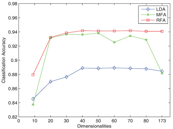
Figure 2.
Classification accuracy obtained by LDA, MFA and RFA on the Ibn Sina dataset.
USPS dataset: The USPS is an U.S. post handwritten digits dataset that contains 7291 training data and 2007 test data from 10 classes and the dimensionality of the data features is 256. Some handwritten digits in the USPS dataset are shown in Figure 3.
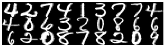
Figure 3.
Sample images from the USPS dataset.
In this experiment, we set the number of the nearest neighbors – k of RFA to 24. The classification accuracies obtained by RFA and the compared algorithms are shown in Figure 4. Because the LDA subspace has a maximum of dimension (C is the number of classes), LDA is only presented with a black star in the figure. We can see that when the dimension is 9, RFA obtains a comparative results with LDA and MFA. When the dimension increases, the results of RFA are always optimal. At the same time, the classification accuracy obtained by RDA is low.
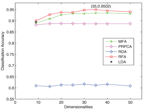
Figure 4.
Classification results obtained by RFA and the compared methods on the USPS dataset.
Figure 5 presents 3D visualization of the learned data representations by RFA, which shows the effect of RFA to obtain better classification boundaries between the classes. In Figure 6, we show the 2D projections of data learned by both RFA and MFA, to further show the effectiveness of RFA. It is easy to see that the samples processed by RFA are less likely to overlap at the boundary, indicating that compared to MFA, RFA preserves more properties that help distinguish the samples.
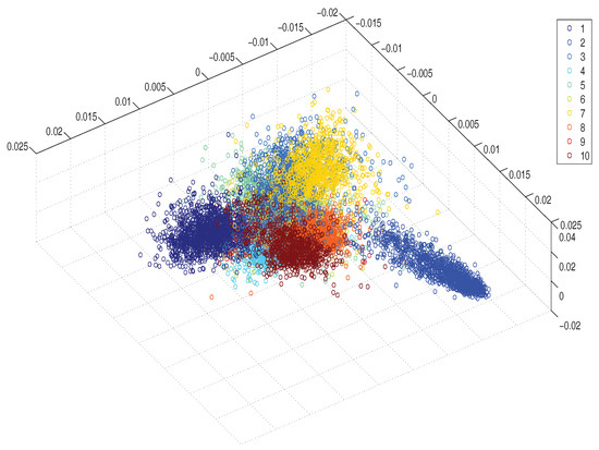
Figure 5.
3D visualization of the mapped data obtained by RFA. Samples of different classes are marked with different colors.
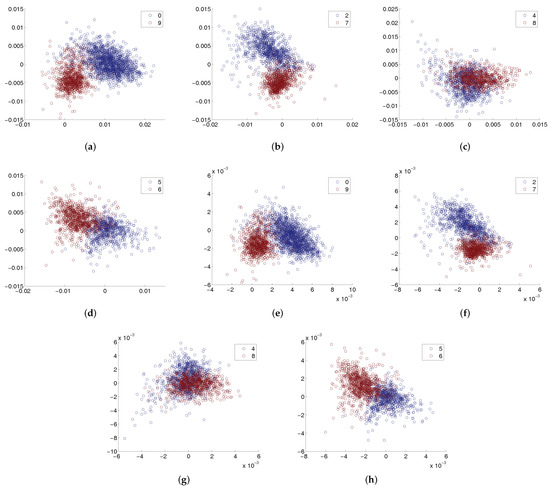
Figure 6.
2D visualization for data pairs. (a–d) are the results obtained by RFA, and (e–h) are the results obtained by MFA.
In addition, the robustness of RFA is tested with respect to and (used to construct the intrinsic and penalty graphs). From Figure 4, it can be seen that RFA obtained the best result when the subspace dimension was 35, with parameter settings = 5, = 20 and k = 24. We fixed k and one of and to obtain the results when another parameter took different values. Figure 7 and Figure 8 show that RFA is very robust.
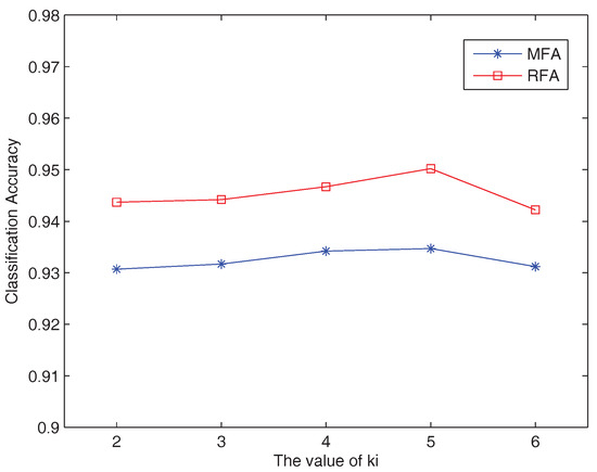
Figure 7.
Classification results obtained by RFA and MFA with different values of on the USPS dataset.
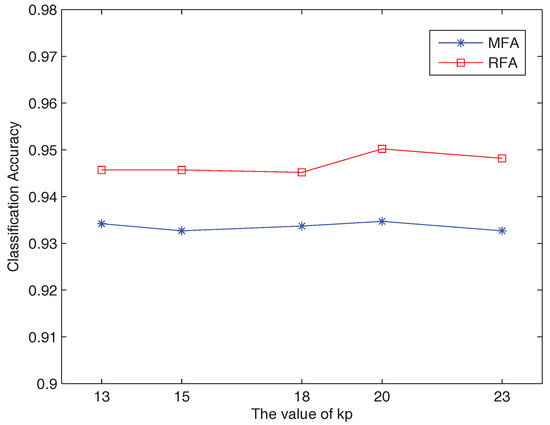
Figure 8.
Classification results obtained by RFA and MFA with different values of on the USPS dataset.
We also selected three document recognition-related datasets from the UCI machine learning repository to further test the effectiveness of RFA. They are Optdigits, Pendigits and Letter. Optdigits was preprocessed by NIST [57] programs to obtain 5620 instances in 8 × 8 dimensions. The Pendigits dataset contains a large number of preprocessed 16-dimensional samples written by 44 different authors, including 7494 training examples and 3498 test samples. Letter consists of 20,000 handwritten characters written by 20 fonts from 26 capital letters in the English alphabet. We used the 5-fold cross-validation for these experiments. Table 2, Table 3 and Table 4 show the classification accuracy and standard deviation obtained on these three datasets and the boldface results are the best ones. We can see that RFA performs consistently better than other compared methods.
Table 2.
Classification results obtained on the Optdigits dataset. The best results are highlighted in boldface.
Table 3.
Classification results obtained on the Pendigits dataset.
Table 4.
Classification results obtained on the Letter dataset.
5.1.2. Comparison on Face Datasets
Here, we tested RFA on the face recognition problems. The PIE and YaleB datasets were used. The details of these two datasets are shown in Table 5. For the corresponding experimental settings, we set the number of the nearest neighbors – k on the PIE dataset to 8 and k on the YaleB dataset to 18.
Table 5.
Statistics of the face recognition datasets.
Considering that RDA cannot perform well on multi-class classification problems, we used LPP instead as a compared method in these experiments. We used the 5-fold cross-validation to decide the value of parameter k for graph construction in LPP. We performed the experiments in different low-dimensional spaces on the PIE and YaleB datasets, and the experimental results are shown in Table 6 and Table 7.
Table 6.
Classification results obtained on the PIE dataset.
Table 7.
Classification results obtained on the YaleB dataset.
We can see from the experimental results that RFA performs very well. Although LPP is an effective dimensionality reduction method for face recognition, RFA is significantly better than LPP. Moreover, RFA obtains comparable results with LDA and MFA. These results demonstrate the effectiveness of RFA in the face recognition applications.
Additionally, convergence of RFA is verified on these two datasets. As illustrated in Figure 9 and Figure 10, the value of (trace ratio) decreases through the iterative procedures until it reaches the global optimal value on both of the two datasets, which clearly shows the convergence of RFA.
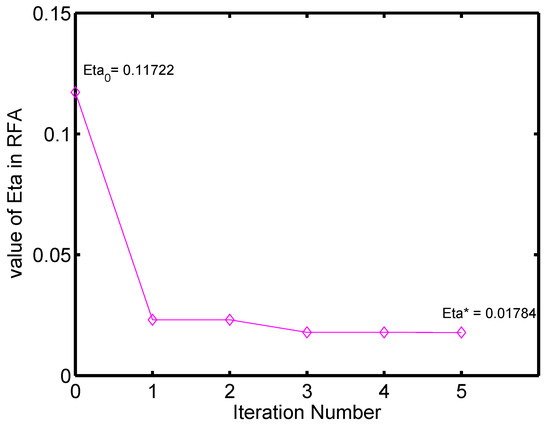
Figure 9.
Changing cave of over the iteration number on the PIE dataset.
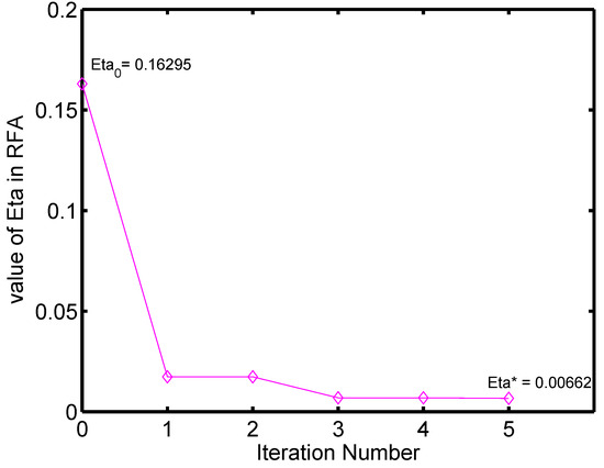
Figure 10.
Changing cave of over the iteration number on the YaleB dataset.
5.1.3. Comparison on Other UCI Datasets
To evaluate the generalization ability of RFA, we conducted experiments on UCI datasets of other fields. The details of the used datasets are shown in Table 8. For the corresponding experimental settings of these four dataset, we set the number of the nearest neighbors – k to 15. For the fairness of comparison, the subspace dimension of each method was set to .
Table 8.
Statistics of the UCI datasets.
The results shown in Table 9 demonstrate the advantage of RFA over the related approaches. It is very effective in a wide range of applications.
Table 9.
Classification results obtained on several UCI datasets.
5.1.4. Comparison on Document Classification and Webpage Classification Problems
As a general dimensionality reduction framework, the relational matrix can be constructed with different strategies. In the previous sections, we considered the relationship between samples based on their class labels or similarity. However, in some complicated problems, relationships may presented in other forms. For example, as indicated in [25], if there is a reference relationship between two papers, they are likely to have the same topic. However, due to the sparse nature of the bag-of-words representation, the similarity between these two papers may be very low. Thus, to further testify RFA, we designed a relational matrix based on the citation relevance between data samples to model RFA, and tested its effectiveness on document classification and webpage classification problems.
For this experiment, we used two datasets, citeseer and WebKB (https://linqs-data.soe.ucsc.edu/public/lbc/, accessed on 19 October 2023). We note that the WebKB dataset contains four subsets: Cornell, Texas, Washington and Wisconsin, and we show the experimental results of these four subsets separately. Each dataset contains bag-of-words representation of documents or webpages and citation links between the instances. Citeseer contains 3312 scientific documents from 6 different classes, and there are 4732 citation relation between the documents. WebKB consists of 877 webpages from 5 different classes, and there are 1608 page links within this dataset. We adopted the same strategy as in PRPCA to construct the relational matrix:
(1) Constructing the adjacent graph according to the relevance between data samples. If there was a citation or link between sample i and j, then ; else, .
(2) Letting , then ,
(3) Defining as the relational matrix in RFA.
We took PRPCA as the baseline method in this part. Experimental results are illustrated in Figure 11; we can see that RFA achieves comparable results with PRPCA in all these five datasets and is even better than PRPCA on some of the datasets.
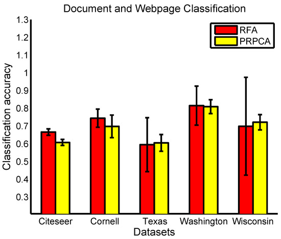
Figure 11.
Classification accuracy and standard deviation obtained by RFA and PRPCA on the document and webpage classification problems.
5.2. Performance of KRFA
To evaluate the efficiency of KRFA, we tested its performance on several benchmark datasets from the UCI machine learning repository. The details of these datasets are shown in Table 10. For the corresponding experimental settings, we set the number of the nearest neighbors – k of these five dataset to 15. To avoid the singular value issue, we adopted KPCA to retain 98% of the variance before formally performing KMFA and KRFA. We used Gaussian kernel in the experiment and for the fairness of the comparison, the subspace dimension of each method was set to . Table 11 shows the comparison results obtained by KRFA, KMFA and RFA.
Table 10.
Statistics of the UCI datasets.
Table 11.
Classification accuracy and standard deviation obtained on several UCI datasets.
As shown in Table 11, the proposed KRFA obtained a comparable and even better result than KMFA. Furthermore, experimental results of KRFA were all better than RFA on the used datasets. That superiority can be especially reflected on the Satimage dataset. The performance of RFA on Satimage was unsatisfactory. However, KRFA conducted effective nonlinear dimensionality reduction and thus obtained good result on the following classification problem. These two points clearly demonstrate the nonlinear dimensionality reduction ability of KRFA.
6. Conclusions
In this paper, we propose a novel and general framework named relational Fisher analysis (RFA) which integrates relational information into the dimensionality reduction models. RFA can be effectively optimized with an iterative method based on trace ratio. For nonlinear dimensionality reduction, we adopt kernel trick to RFA and design its kernel version named KRFA. Extensive experiments demonstrate that RFA and KRFA outperform other related dimensionality reduction algorithms in most cases. In future work, we plan to extend this research in the following aspects: (1) Exploiting efficient relationship metric for different relational data to further test the effectiveness of the proposed RFA model; (2) Further extending the formulation of RFA for semi-supervised learning; and (3) Extending RFA for tensor representation learning and applying it to tensor analysis problems.
Author Contributions
Conceptualization, L.-N.W. and G.Z.; methodology, L.-N.W. and M.C.; software, Y.S.; validation, L.-N.W. and M.C.; formal analysis, G.Z.; investigation, L.-N.W.; resources, G.Z.; data curation, Y.S.; writing—original draft preparation, L.-N.W., Y.S. and G.Z.; writing—review and editing, M.C.; visualization, Y.S.; supervision, G.Z.; project administration, M.C.; funding acquisition, G.Z. All authors have read and agreed to the published version of the manuscript.
Funding
This work was partially supported by the National Key Research and Development Program of China under Grant No. 2018AAA0100400, HY Project under Grant No. LZY2022033004, the Natural Science Foundation of Shandong Province under Grants No. ZR2020MF131 and No. ZR2021ZD19, the Science and Technology Program of Qingdao under Grant No. 21-1-4-ny-19-nsh, and Project of Associative Training of Ocean University of China under Grant No. 202265007.
Institutional Review Board Statement
Not applicable.
Informed Consent Statement
Not applicable.
Data Availability Statement
The data used in this work were public on the Internet and no new data were created.
Acknowledgments
We thank “Qingdao AI Computing Center” and “Eco-Innovation Center” for providing inclusive computing power and technical support of MindSpore during the completion of this paper.
Conflicts of Interest
The authors declare no conflict of interest.
References
- Jolliffe, I. Principal Component Analysis; Wiley Online Library: Hoboken, NJ, USA, 2002. [Google Scholar]
- Martínez, A.M.; Kak, A.C. Pca versus lda. IEEE Trans. Pattern Anal. Mach. Intell. 2001, 23, 228–233. [Google Scholar] [CrossRef]
- Turk, M.A.; Pentland, A.P. Face recognition using eigenfaces. In Proceedings of the 1991 IEEE Computer Society Conference on Computer Vision and Pattern Recognition, Maui, HI, USA, 3–6 June 1991; pp. 586–591. [Google Scholar]
- Fukunaga, K. Introduction to Statistical Pattern Recognition; Academic Press: Cambridge, MA, USA, 2013. [Google Scholar]
- Ye, J.; Janardan, R.; Park, C.H.; Park, H. An optimization criterion for generalized discriminant analysis on undersampled problems. IEEE Trans. Pattern Anal. Mach. Intell. 2004, 26, 982–994. [Google Scholar] [PubMed]
- Lu, J.; Plataniotis, K.N.; Venetsanopoulos, A.N. Face recognition using LDA-based algorithms. IEEE Trans. Neural Netw. 2003, 14, 195–200. [Google Scholar] [PubMed]
- Fisher, R.A. The use of multiple measurements in taxonomic problems. Ann. Eugen. 1936, 7, 179–188. [Google Scholar] [CrossRef]
- Schölkopf, B.; Smola, A.J.; Müller, K. Nonlinear Component Analysis as a Kernel Eigenvalue Problem. Neural Comput. 1998, 10, 1299–1319. [Google Scholar] [CrossRef]
- Baudat, G.; Anouar, F. Generalized Discriminant Analysis Using a Kernel Approach. Neural Comput. 2000, 12, 2385–2404. [Google Scholar] [CrossRef]
- Zhao, H.; Wang, Z.; Nie, F. A New Formulation of Linear Discriminant Analysis for Robust Dimensionality Reduction. IEEE Trans. Knowl. Data Eng. 2018, 31, 629–640. [Google Scholar] [CrossRef]
- Tenenbaum, J.B.; de Silva, V.; Langford, J.C. A Global Geometric Framework for Nonlinear Dimensionality Reduction. Science 2000, 290, 2319–2323. [Google Scholar] [CrossRef]
- Roweis, S.T.; Saul, L.K. Nonlinear Dimensionality Reduction by Locally Linear Embedding. Science 2000, 290, 2323–2326. [Google Scholar] [CrossRef]
- Belkin, M.; Niyogi, P. Laplacian Eigenmaps for Dimensionality Reduction and Data Representation. Neural Comput. 2003, 15, 1373–1396. [Google Scholar] [CrossRef]
- Yan, S.; Xu, D.; Zhang, B.; Zhang, H.J.; Yang, Q.; Lin, S. Graph Embedding and Extensions: A General Framework for Dimensionality Reduction. IEEE Trans. Pattern Anal. Mach. Intell. 2007, 29, 40–51. [Google Scholar] [CrossRef] [PubMed]
- He, X.; Niyogi, P. Locality Preserving Projections. In Proceedings of the 16th International Conference on Neural Information Processing Systems, Whistler, BC, Canada, 9–11 December 2003; pp. 153–160. [Google Scholar]
- Wong, W.K.; Zhao, H. Supervised optimal locality preserving projection. Pattern Recognit. 2012, 45, 186–197. [Google Scholar] [CrossRef]
- Chen, J.; Liu, Y. Locally linear embedding: A survey. Artif. Intell. Rev. 2011, 36, 29–48. [Google Scholar] [CrossRef]
- Wang, Q.; Chen, K. Zero-Shot Visual Recognition via Bidirectional Latent Embedding. Int. J. Comput. Vis. 2017, 124, 356–383. [Google Scholar] [CrossRef]
- Chang, J.; Blei, D.M. Relational Topic Models for Document Networks. J. Mach. Learn. Res. Proc. Track 2009, 5, 81–88. [Google Scholar]
- Chang, J.; Boyd-Graber, J.L.; Blei, D.M. Connections between the Lines: Augmenting Social Networks with Text. In Proceedings of the 15th ACM SIGKDD International Conference on Knowledge Discovery and Data Mining, Paris, France, 28 June–1 July 2009; pp. 169–178. [Google Scholar]
- Peel, L. Graph-based semi-supervised learning for relational networks. arXiv 2016, arXiv:1612.05001. [Google Scholar]
- Yang, Z.; Cohen, W.; Salakhutdinov, R. Revisiting semi-supervised learning with graph embeddings. arXiv 2016, arXiv:1603.08861. [Google Scholar]
- Weston, J.; Ratle, F.; Mobahi, H.; Collobert, R. Deep learning via semi-supervised embedding. In Neural Networks: Tricks of the Trade; Springer: Berlin/Heidelberg, Germany, 2012; pp. 639–655. [Google Scholar]
- Duin, R.P.W.; Pekalska, E.; de Ridder, D. Relational Discriminant Analysis. Pattern Recognit. Lett. 1999, 20, 1175–1181. [Google Scholar] [CrossRef]
- Li, W.J.; Yeung, D.Y.; Zhang, Z. Probabilistic Relational PCA. In Proceedings of the 22nd International Conference on Neural Information Processing Systems, Vancouver, BC, Canada, 7–10 December 2009; pp. 1123–1131. [Google Scholar]
- Gao, K.; Liu, B.; Yu, X.; Qin, J.; Zhang, P.; Tan, X. Deep Relation Network for Hyperspectral Image Few-Shot Classification. Remote Sens. 2020, 12, 923. [Google Scholar] [CrossRef]
- Chen, S.; Yao, T.; Chen, Y.; Ding, S.; Li, J.; Ji, R. Local Relation Learning for Face Forgery Detection. In Proceedings of the Thirty-Fifth AAAI Conference on Artificial Intelligence, Virtually, 2–9 February 2021; pp. 1081–1088. [Google Scholar]
- Cho, M.; Kim, M.; Hwang, S.; Park, C.; Lee, K.; Lee, S. Look Around for Anomalies: Weakly-Supervised Anomaly Detection via Context-Motion Relational Learning. In Proceedings of the 2023 IEEE/CVF Conference on Computer Vision and Pattern Recognition (CVPR), Vancouver, BC, Canada, 17–24 June 2023; pp. 12137–12146. [Google Scholar]
- Ma, R.; Mei, B.; Ma, Y.; Zhang, H.; Liu, M.; Zhao, L. One-shot relational learning for extrapolation reasoning on temporal knowledge graphs. Data Min. Knowl. Discov. 2023, 37, 1591–1608. [Google Scholar] [CrossRef]
- Li, X.; Ma, J.; Yu, J.; Zhao, M.; Yu, M.; Liu, H.; Ding, W.; Yu, R. A structure-enhanced generative adversarial network for knowledge graph zero-shot relational learning. Inf. Sci. 2023, 629, 169–183. [Google Scholar] [CrossRef]
- Zhong, G.; Shi, Y.; Cheriet, M. Relational Fisher analysis: A general framework for dimensionality reduction. In Proceedings of the 2016 International Joint Conference on Neural Networks (IJCNN), Vancouver, BC, Canada, 24–29 July 2016; pp. 2244–2251. [Google Scholar]
- He, X.; Yan, S.; Hu, Y.; Zhang, H.J. Learning a Locality Preserving Subspace for Visual Recognition. In Proceedings of the IEEE International Conference on Computer Vision, Nice, France, 13–16 October 2003; Volume 1, pp. 385–392. [Google Scholar]
- Wang, H.; Yan, S.; Xu, D.; Tang, X.; Huang, T.S. Trace Ratio vs. Ratio Trace for Dimensionality Reduction. In Proceedings of the 2007 IEEE Computer Society Conference on Computer Vision and Pattern Recognition (CVPR 2007), Minneapolis, MN, USA, 18–23 June 2007. [Google Scholar]
- Nie, F.; Xiang, S.; Jia, Y.; Zhang, C.; Yan, S. Trace Ratio Criterion for Feature Selection. In Proceedings of the Twenty-Third AAAI Conference on Artificial Intelligence, Chicago, IL, USA, 13–17 July 2008; Volume 2, pp. 671–676. [Google Scholar]
- Zhong, G.; Ling, X. The necessary and sufficient conditions for the existence of the optimal solution of trace ratio problems. In Proceedings of the Chinese Conference on Pattern Recognition, Chengdu, China, 5–7 November 2016; Springer: Berlin/Heidelberg, Germany, 2016; pp. 742–751. [Google Scholar]
- Duin, R.P.; de Ridder, D.; Tax, D.M. Experiments with a featureless approach to pattern recognition. Pattern Recognit. Lett. 1997, 18, 1159–1166. [Google Scholar] [CrossRef]
- Duin, R.P. Relational discriminant analysis and its large sample size problem. In Proceedings of the 14th International Conference on Pattern Recognition, Washington, DC, USA, 16–20 August 1998; Volume 1, pp. 445–449. [Google Scholar]
- Ypma, A.; Duin, R.P. Support objects for domain approximation. In Proceedings of the 8th International Conference on Artificial Neural Networks, Skövde, Sweden, 2–4 September 1998; Springer: Berlin/Heidelberg, Germany, 1998; pp. 719–724. [Google Scholar]
- Borg, I.; Groenen, P.J. Modern Multidimensional Scaling: Theory and Applications; Springer Science & Business Media: Berlin/Heidelberg, Germany, 2005. [Google Scholar]
- Sammon, J., Jr. A nonlinear structure analysis mapping for data. IEEE Trans. Comp. 1969, C-18, 401–409. [Google Scholar]
- Niemann, H. Linear and nonlinear mapping of patterns. Pattern Recognit. 1980, 12, 83–87. [Google Scholar] [CrossRef]
- Paccanaro, A.; Hinton, G.E. Learning Distributed Representations of Concepts Using Linear Relational Embedding. IEEE Trans. Knowl. Data Eng. 2001, 13, 232–244. [Google Scholar] [CrossRef]
- Wang, H.; Li, W. Relational Collaborative Topic Regression for Recommender Systems. IEEE Trans. Knowl. Data Eng. 2015, 27, 1343–1355. [Google Scholar] [CrossRef]
- Xuan, J.; Lu, J.; Zhang, G.; Xu, R.Y.D.; Luo, X. Bayesian Nonparametric Relational Topic Model through Dependent Gamma Processes. IEEE Trans. Knowl. Data Eng. 2017, 29, 1357–1369. [Google Scholar] [CrossRef]
- Jia, Y.; Nie, F.; Zhang, C. Trace Ratio Problem Revisited. IEEE Trans. Neural Networks 2009, 20, 729–735. [Google Scholar]
- Xiang, S.; Nie, F.; Zhang, C. Learning A Mahalanobis Distance Metric for Data Clustering and Classification. Pattern Recognit. 2008, 41, 3600–3612. [Google Scholar] [CrossRef]
- Nie, F.; Xiang, S.; Jia, Y.; Zhang, C. Semi-supervised Orthogonal Discriminant Analysis via Label Propagation. Pattern Recognit. 2009, 42, 2615–2627. [Google Scholar] [CrossRef]
- Zhao, M.B.; Zhang, Z.; Chow, T.W.S. Trace Ratio Criterion Based Generalized Discriminative Learning for Semi-supervised Dimensionality Reduction. Pattern Recognit. 2012, 45, 1482–1499. [Google Scholar] [CrossRef]
- Moghaddam, R.F.; Cheriet, M.; Milo, T.; Wisnovsky, R. A Prototype System for Handwritten Sub-word Recognition: Toward Arabic-manuscript Transliteration. In Proceedings of the 2012 11th International Conference on Information Science, Signal Processing and Their Applications (ISSPA), Montreal, QC, Canada, 2–5 July 2012; pp. 1198–1204. [Google Scholar]
- Lichman, M. UCI Machine Learning Repository, 2013. Available online: https://archive.ics.uci.edu/ (accessed on 19 October 2023).
- Gross, R. Face Databases. In Handbook of Face Recognition; Li, S.Z., Jain, A.K., Eds.; Springer: Berlin/Heidelberg, Germany, 2005. [Google Scholar]
- Cai, D.; He, X.; Hu, Y.; Han, J.; Huang, T. Learning a Spatially Smooth Subspace for Face Recognition. In Proceedings of the 2007 IEEE Computer Society Conference on Computer Vision and Pattern Recognition (CVPR 2007), Minneapolis, MN, USA, 18–23 June 2007. [Google Scholar]
- Cai, D.; He, X.; Han, J. Spectral Regression for Efficient Regularized Subspace Learning. In Proceedings of the 11th International Conference on Computer Vision, ICCV 2007, Rio de Janeiro, Brazil, 14–20 October 2007. [Google Scholar]
- Cai, D.; He, X.; Han, J.; Zhang, H.J. Orthogonal Laplacianfaces for face recognition. IEEE Trans. Image Process. 2006, 15, 3608–3614. [Google Scholar] [CrossRef]
- Zheng, Y.; Cai, Y.; Zhong, G.; Chherawala, Y.; Shi, Y.; Dong, J. Stretching Deep Architectures for Text Recognition. In Proceedings of the 2015 13th International Conference on Document Analysis and Recognition (ICDAR), Tunis, Tunisia, 23–26 August 2015; pp. 236–240. [Google Scholar]
- Srivastava, A.; Klassen, E.; Joshi, S.H.; Jermyn, I.H. Shape Analysis of Elastic Curves in Euclidean Spaces. IEEE Trans. Pattern Anal. Mach. Intell. 2011, 33, 1415–1428. [Google Scholar] [CrossRef]
- Garris, M.D.; Blue, J.L.; Candela, G.T.; Dimmick, D.L.; Geist, J.; Grother, P.J.; Janet, S.A.; Wilson, C.L. NIST Form-Based Handprint Recognition System; NIST Interagency/Internal Report (NISTIR); National Institute of Standards and Technology: Gaithersburg, MD, USA, 1994. [Google Scholar]
Disclaimer/Publisher’s Note: The statements, opinions and data contained in all publications are solely those of the individual author(s) and contributor(s) and not of MDPI and/or the editor(s). MDPI and/or the editor(s) disclaim responsibility for any injury to people or property resulting from any ideas, methods, instructions or products referred to in the content. |
© 2023 by the authors. Licensee MDPI, Basel, Switzerland. This article is an open access article distributed under the terms and conditions of the Creative Commons Attribution (CC BY) license (https://creativecommons.org/licenses/by/4.0/).