
Automatic Multiorgan Segmentation in Pelvic Region with Convolutional Neural Networks on 0.35 T MR-Linac Images

 , , ,
, , , 
Abstract
:1. Introduction
2. Materials and Methods
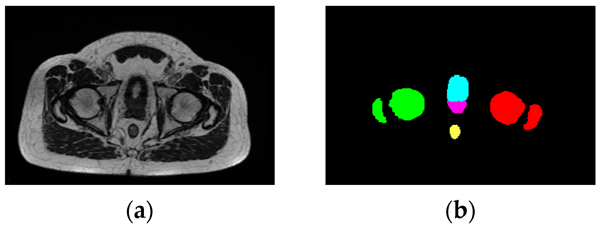
2.1. Dataset
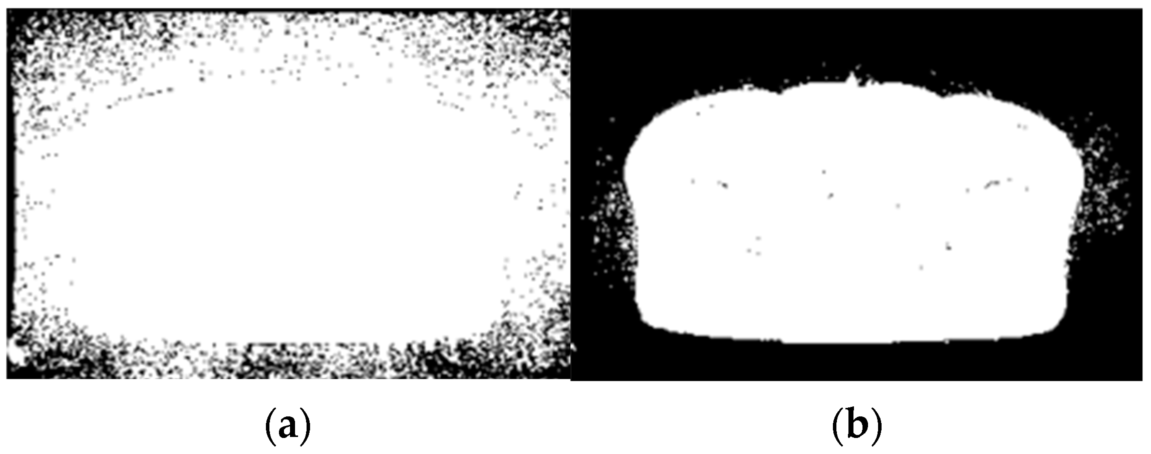
2.2. Preprocessing
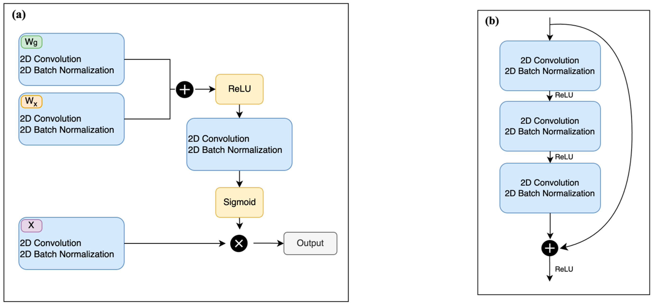
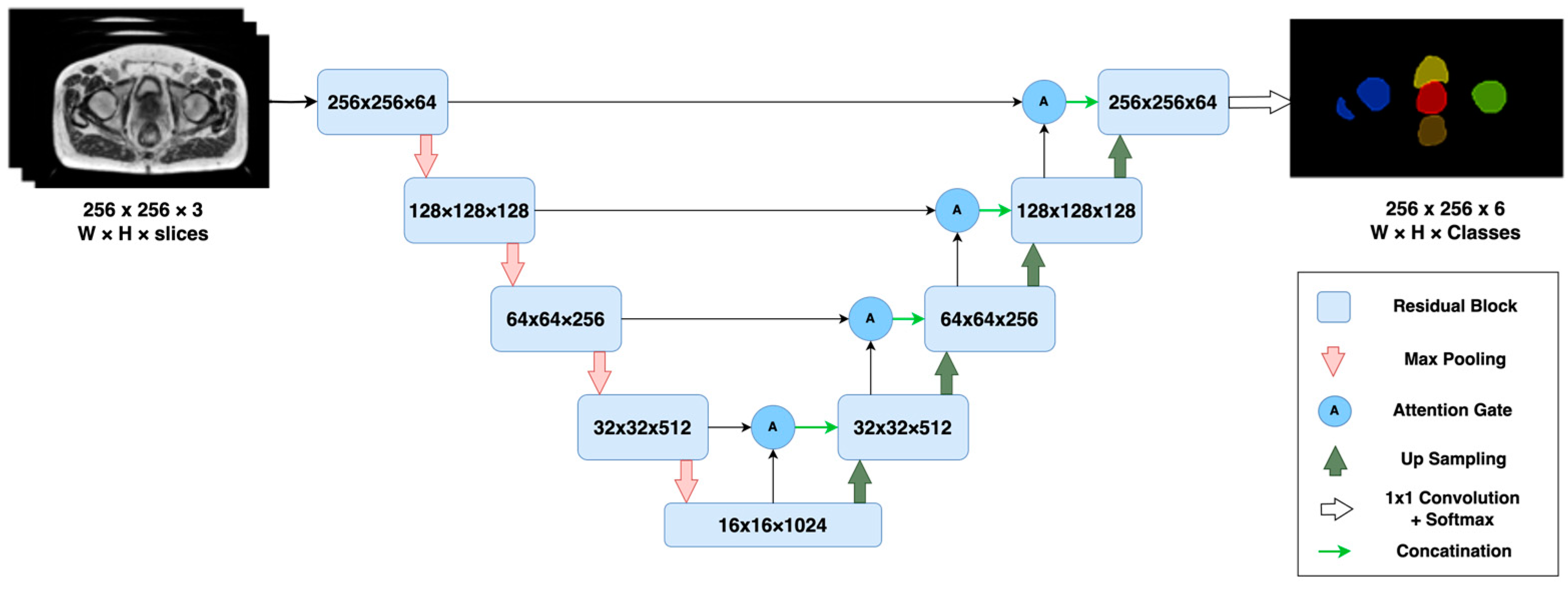
2.3. Residual Attention U-Net Network
2.4. Post-Processing
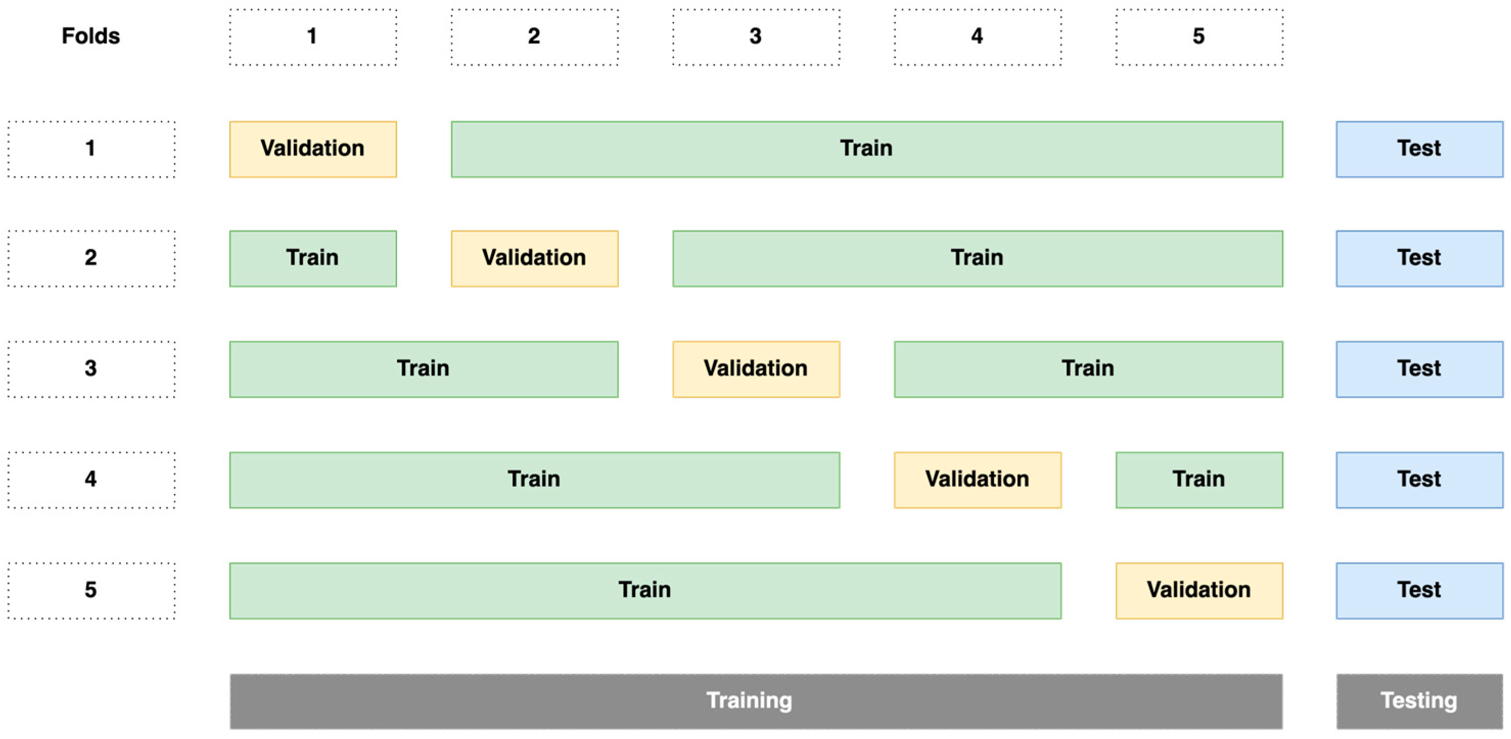
2.5. Evaluation of the Segmentation Algorithm
2.6. Computing Environment
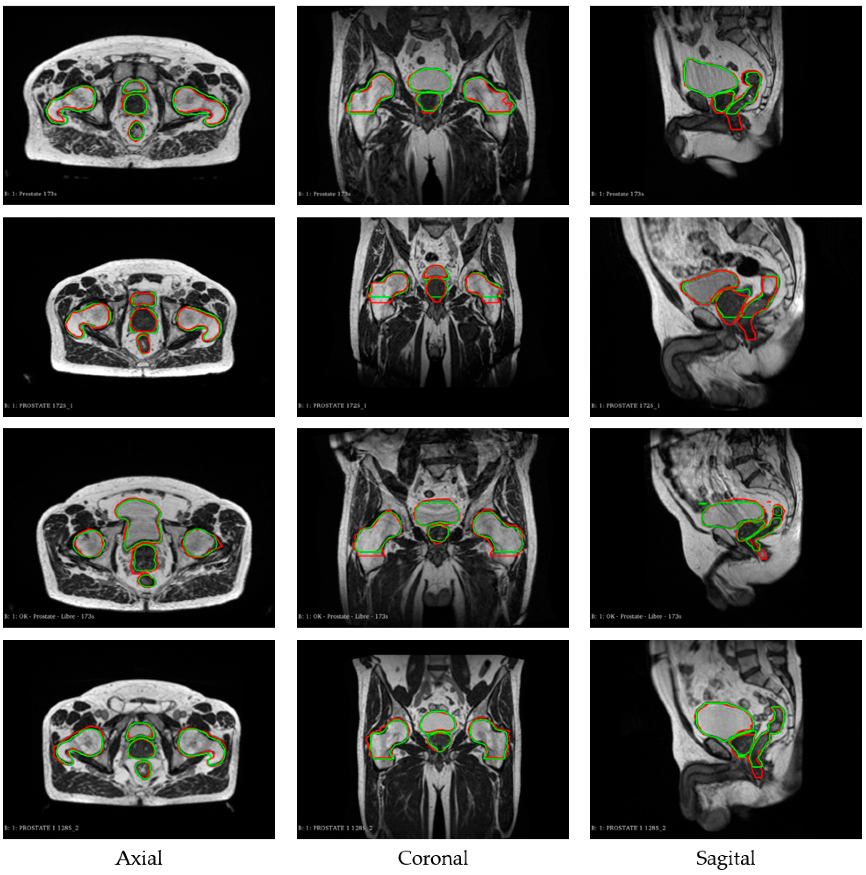
3. Results
4. Discussion
5. Conclusions
Author Contributions
Funding
Institutional Review Board Statement
Data Availability Statement
Conflicts of Interest
References
- Boehmer, D.; Maingon, P.; Poortmans, P.; Baron, M.-H.; Miralbell, R.; Remouchamps, V.; Scrase, C.; Bossi, A.; Bolla, M. Guidelines for primary radiotherapy of patients with prostate cancer. Radiother. Oncol. 2006, 79, 259–269. [Google Scholar] [CrossRef] [PubMed]
- Segedin, B.; Petric, P. Uncertainties in target volume delineation in radiotherapy—Are they relevant and what can we do about them? Radiol. Oncol. 2016, 50, 254–262. [Google Scholar] [CrossRef] [PubMed]
- Gunnlaugsson, A.; Persson, E.; Gustafsson, C.; Kjellén, E.; Ambolt, P.; Engelholm, S.; Nilsson, P.; Olsson, L.E. Target definition in radiotherapy of prostate cancer using magnetic resonance imaging only workflow. Phys. Imaging Radiat. Oncol. 2019, 9, 89–91. [Google Scholar] [CrossRef] [PubMed]
- Kupelian, P.; Sonke, J.-J. Magnetic Resonance–Guided Adaptive Radiotherapy: A Solution to the Future. Semin. Radiat. Oncol. 2014, 24, 227–232. [Google Scholar] [CrossRef] [PubMed]
- Pollard, J.M.; Wen, Z.; Sadagopan, R.; Wang, J.; Ibbott, G.S. The future of image-guided radiotherapy will be MR guided. Br. J. Radiol. 2017, 90, 20160667. [Google Scholar] [CrossRef]
- Tyagi, N.; Zelefsky, M.J.; Wibmer, A.; Zakian, K.; Burleson, S.; Happersett, L.; Halkola, A.; Kadbi, M.; Hunt, M. Clinical experience and workflow challenges with magnetic resonance-only radiation therapy simulation and planning for prostate cancer. Phys. Imaging Radiat. Oncol. 2020, 16, 43–49. [Google Scholar] [CrossRef]
- Greer, P.; Martin, J.; Sidhom, M.; Hunter, P.; Pichler, P.; Choi, J.H.; Best, L.; Smart, J.; Young, T.; Jameson, M.; et al. A multi-center prospective study for implementation of an MRI-only prostate treatment planning work-flow. Front. Oncol. 2019, 9, 826. [Google Scholar] [CrossRef]
- Ménard, C.; Paulson, E.; Nyholm, T.; McLaughlin, P.; Liney, G.; Dirix, P.; van der Heide, U.A. Role of Prostate MR Imaging in Radiation Oncology. Radiol. Clin. N. Am. 2018, 56, 319–325. [Google Scholar] [CrossRef]
- Yuan, J.; Poon, D.M.C.; Lo, G.; Wong, O.L.; Cheung, K.Y.; Yu, S.K. A narrative review of MRI acquisition for MR-guided-radiotherapy in prostate cancer. Quant. Imaging Med. Surg. 2022, 12, 1585–1607. [Google Scholar] [CrossRef]
- Kishan, A.U.; Ma, T.M.; Lamb, J.M.; Casado, M.; Wilhalme, H.; Low, D.A.; Sheng, K.; Sharma, S.; Nickols, N.G.; Pham, J.; et al. Magnetic Resonance Imaging–Guided vs Computed Tomography–Guided Stereotactic Body Radiotherapy for Prostate Cancer. JAMA Oncol. 2023, 9, 365–373. [Google Scholar] [CrossRef]
- Ma, T.; Neylon, J.; Savjani, R.; Low, D.; Steinberg, M.; Cao, M.; Kishan, A. Treatment Delivery Gating of MRI-Guided Stereotactic Radiotherapy for Prostate Cancer: An Exploratory Analysis of a Phase III Randomized Trial of CT-Vs. MR-Guided Radiotherapy (MIRAGE). Int. J. Radiat. Oncol. 2023, 117, e692–e693. [Google Scholar] [CrossRef]
- Klüter, S. Technical design and concept of a 0.35 T MR-Linac. Clin. Transl. Radiat. Oncol. 2019, 18, 98–101. [Google Scholar] [CrossRef] [PubMed]
- Cardenas, C.E.; Yang, J.; Anderson, B.M.; Court, L.E.; Brock, K.B. Advances in Auto-Segmentation. Semin. Radiat. Oncol. 2019, 29, 185–197. [Google Scholar] [CrossRef] [PubMed]
- Kalantar, R.; Lin, G.; Winfield, J.M.; Messiou, C.; Lalondrelle, S.; Blackledge, M.D.; Koh, D.-M. Automatic Segmentation of Pelvic Cancers Using Deep Learning: State-of-the-Art Approaches and Challenges. Diagnostics 2021, 11, 1964. [Google Scholar] [CrossRef] [PubMed]
- Almeida, G.; Tavares, J.M.R. Deep Learning in Radiation Oncology Treatment Planning for Prostate Cancer: A Systematic Review. J. Med. Syst. 2020, 44, 179. [Google Scholar] [CrossRef] [PubMed]
- Fu, Y.; Lei, Y.; Wang, T.; Curran, W.J.; Liu, T.; Yang, X. A review of deep learning based methods for medical image multi-organ segmentation. Phys. Med. 2021, 85, 107–122. [Google Scholar] [CrossRef]
- Khan, Z.; Yahya, N.; Alsaih, K.; Al-Hiyali, M.I.; Meriaudeau, F. Recent Automatic Segmentation Algorithms of MRI Prostate Regions: A Review. IEEE Access 2021, 9, 97878–97905. [Google Scholar] [CrossRef]
- Valentini, V.; Boldrini, L.; Damiani, A.; Muren, L.P. Recommendations on how to establish evidence from auto-segmentation software in radiotherapy. Radiother. Oncol. 2014, 112, 317–320. [Google Scholar] [CrossRef]
- Cusumano, D.; Boldrini, L.; Dhont, J.; Fiorino, C.; Green, O.; Güngör, G.; Jornet, N.; Klüter, S.; Landry, G.; Mattiucci, G.C.; et al. Artificial Intelligence in magnetic Resonance guided Radiotherapy: Medical and physical considerations on state of art and future perspectives. Phys. Med. 2021, 85, 175–191. [Google Scholar] [CrossRef]
- Cabezas, M.; Oliver, A.; Lladó, X.; Freixenet, J.; Cuadra, M.B. A review of atlas-based segmentation for magnetic resonance brain images. Comput. Methods Progr. Biomed. 2011, 104, e158–e177. [Google Scholar] [CrossRef]
- Wang, H.; Yushkevich, P.A. Multi-atlas Segmentation without Registration: A Supervoxel-Based Approach. Med. Image Comput. Comput.-Assist. Interv. 2013, 16, 535–542. [Google Scholar]
- Heckemann, R.A.; Hajnal, J.V.; Aljabar, P.; Rueckert, D.; Hammers, A. Automatic anatomical brain MRI segmentation combining label propagation and decision fusion. NeuroImage 2006, 33, 115–126. [Google Scholar] [CrossRef] [PubMed]
- Martínez, F.; Romero, E.; Dréan, G.; Simon, A.; Haigron, P.; de Crevoisier, R.; Acosta, O. Segmentation of pelvic structures for planning CT using a geometrical shape model tuned by a multi-scale edge detector. Phys. Med. Biol. 2014, 59, 1471–1484. [Google Scholar] [CrossRef] [PubMed]
- Iglesias, J.E.; Sabuncu, M.R. Multi-atlas segmentation of biomedical images: A survey. Med. Image Anal. 2015, 24, 205–219. [Google Scholar] [CrossRef] [PubMed]
- Shelhamer, E.; Long, J.; Darrell, T. Fully convolutional networks for semantic segmentation. IEEE Trans. Pattern Anal. Mach. Intell. 2017, 39, 640–651. [Google Scholar] [CrossRef]
- Ronneberger, O.; Fischer, P.; Brox, T. U-Net: Convolutional Networks for Biomedical Image Segmentation; Lecture Notes in Computer Science (Including Subseries Lecture Notes in Artificial Intelligence and Lecture Notes in Bioinformatics); Springer: Cham, Switzerland, 2015; Volume 9351, pp. 234–241. Available online: https://arxiv.org/abs/1505.04597v1 (accessed on 20 June 2023).
- Zhou, Z.; Siddiquee, M.M.R.; Tajbakhsh, N.; Liang, J. UNet++: A Nested U-Net Architecture for Medical Image Seg-mentation. arXiv 2018, arXiv:1807.10165. [Google Scholar]
- Cao, Y.; Liu, S.; Peng, Y.; Li, J. DenseUNet: Densely connected UNet for electron microscopy image segmentation. IET Image Process. 2020, 14, 2682–2689. [Google Scholar] [CrossRef]
- Chen, X.; Yao, L.; Zhang, Y. Residual Attention U-Net for Automated Multi-Class Segmentation of COVID-19 Chest CT Images. arXiv 2020, arXiv:2004.05645. [Google Scholar]
- Oktay, O.; Schlemper, J.; Le Folgoc, L.; Lee, M.; Heinrich, M.; Misawa, K.; Mori, K.; McDonagh, S.; Hammerla, N.Y.; Kainz, B.; et al. Attention U-Net: Learning Where to Look for the Pancreas. arXiv 2018, arXiv:1804.03999. [Google Scholar]
- Ben-Cohen, A.; Diamant, I.; Klang, E.; Amitai, M.; Greenspan, H. Fully Convolutional Network for Liver Segmentation and Lesions Detection; Lecture Notes in Computer Science (including subseries Lecture Notes in Artificial Intelligence and Lecture Notes in Bioinformatics); Springer: Berlin/Heidelberg, Germany, 2016; Volume 10008, pp. 77–85. [Google Scholar] [CrossRef]
- Minnema, J.; Wolff, J.; Koivisto, J.; Lucka, F.; Batenburg, K.J.; Forouzanfar, T.; van Eijnatten, M. Comparison of convolutional neural network training strategies for cone-beam CT image segmentation. Comput. Methods Progr. Biomed. 2021, 207, 106192. [Google Scholar] [CrossRef]
- Maji, D.; Sigedar, P.; Singh, M. Attention Res-UNet with Guided Decoder for semantic segmentation of brain tumors. Biomed. Signal Process. Control 2021, 71, 103077. [Google Scholar] [CrossRef]
- He, K.; Zhang, X.; Ren, S.; Sun, J. Deep residual learning for image recognition. In Proceedings of the IEEE Computer Society Conference on Computer Vision and Pattern Recognition (CVPR), Las Vegas, NV, USA, 27–30 June 2016; pp. 770–778. [Google Scholar] [CrossRef]
- Aldoj, N.; Biavati, F.; Michallek, F.; Stober, S.; Dewey, M. Automatic prostate and prostate zones segmentation of magnetic resonance images using DenseNet-like U-net. Sci. Rep. 2020, 10, 14315. [Google Scholar] [CrossRef] [PubMed]
- Huang, G.; Liu, Z.; van der Maaten, L.; Weinberger, K.Q. Densely Connected Convolutional Networks. arXiv 2016, arXiv:1608.06993. [Google Scholar]
- Elguindi, S.; Zelefsky, M.J.; Jiang, J.; Veeraraghavan, H.; Deasy, J.O.; Hunt, M.A.; Tyagi, N. Deep learning-based auto-segmentation of targets and organs-at-risk for magnetic resonance imaging only planning of prostate radiotherapy. Phys. Imaging Radiat. Oncol. 2019, 12, 80–86. [Google Scholar] [CrossRef] [PubMed]
- Chen, L.C.; Zhu, Y.; Papandreou, G.; Schroff, F.; Adam, H. Encoder-Decoder with Atrous Separable Convolution for Semantic Image Segmentation; Lecture Notes in Computer Science (including subseries Lecture Notes in Artificial Intelligence and Lecture Notes in Bioinformatics); Springer: Berlin/Heidelberg, Germany, 2018; Volume 11211, pp. 833–851. [Google Scholar] [CrossRef]
- Alkadi, R.; El-Baz, A.; Taher, F.; Werghi, N. A 2.5D Deep Learning-Based Approach for Prostate Cancer Detection on T2-Weighted Magnetic Resonance Imaging. In Proceedings of the 2018 European Conference on Computer Vision, Munich, Germany, 8–14 September 2018; pp. 734–739. [Google Scholar]
- Huang, S.; Cheng, Z.; Lai, L.; Zheng, W.; He, M.; Li, J.; Zeng, T.; Huang, X.; Yang, X. Integrating multiple MRI sequences for pelvic organs segmentation via the attention mechanism. Med. Phys. 2021, 48, 7930–7945. [Google Scholar] [CrossRef]
- Marage, L.; Walker, P.-M.; Boudet, J.; Fau, P.; Debuire, P.; Clausse, E.; Petitfils, A.; Aubignac, L.; Rapacchi, S.; Bessieres, I. Characterisation of a split gradient coil design induced systemic imaging artefact on 0.35 T MR-linac systems. Phys. Med. Biol. 2022, 68, 01NT03. [Google Scholar] [CrossRef]
- Lin, T.Y.; Goyal, P.; Girshick, R.; He, K.; Dollar, P. Focal Loss for Dense Object Detection. IEEE Trans. Pattern Anal. Mach. Intell. 2017, 42, 318–327. [Google Scholar] [CrossRef]
- Buda, M.; Maki, A.; Mazurowski, M.A. A systematic study of the class imbalance problem in convolutional neural networks. Neural Netw. 2018, 106, 249–259. [Google Scholar] [CrossRef]
- Kingma, D.P.; Ba, J.L. Adam: A Method for Stochastic Optimization. In Proceedings of the 3rd International Conference on Learning Representations, ICLR 2015-Conference Track Proceedings, San Diego, CA, USA, 7–9 May 2015. [Google Scholar] [CrossRef]
- Lundervold, A.S.; Lundervold, A. An overview of deep learning in medical imaging focusing on MRI. Z. Med. Phys. 2018, 29, 102–127. [Google Scholar] [CrossRef]
- Schenk, A.; Prause, G.; Peitgen, H.O. Efficient Semiautomatic Segmentation of 3D Objects in Medical Images; Lecture Notes in Computer Science (including subseries Lecture Notes in Artificial Intelligence and Lecture Notes in Bioinformatics); Springer: Berlin/Heidelberg, Germany, 2000; Volume 1935, pp. 186–195. [Google Scholar] [CrossRef]
- Samarasinghe, G.; Jameson, M.; Vinod, S.; Field, M.; Dowling, J.; Sowmya, A.; Holloway, L. Deep learning for segmentation in radiation therapy planning: A review. J. Med. Imaging Radiat. Oncol. 2021, 65, 578–595. [Google Scholar] [CrossRef]
- Zheng, H.; Qian, L.; Qin, Y.; Gu, Y.; Yang, J. Improving the slice interaction of 2.5D CNN for automatic pancreas segmentation. Med. Phys. 2020, 47, 5543–5554. [Google Scholar] [CrossRef] [PubMed]
- Li, J.; Liao, G.; Sun, W.; Sun, J.; Sheng, T.; Zhu, K.; von Deneen, K.M.; Zhang, Y. A 2.5D semantic segmentation of the pancreas using attention guided dual context embedded U-Net. Neurocomputing 2022, 480, 14–26. [Google Scholar] [CrossRef]
- Hu, K.; Liu, C.; Yu, X.; Zhang, J.; He, Y.; Zhu, H. A 2.5D Cancer Segmentation for MRI Images Based on U-Net. In Proceedings of the 2018 5th International Conference on Information Science and Control Engineering (ICISCE), ICISCE 2018, Zhengzhou, China, 20–22 July 2018; pp. 6–10. [Google Scholar]
- Battulga, B.; Konishi, T.; Tamura, Y.; Moriguchi, H. The Effectiveness of an Interactive 3-Dimensional Computer Graphics Model for Medical Education. Interact. J. Med. Res. 2012, 1, e2. [Google Scholar] [CrossRef]
- Sun, L.; Guo, C.; Yao, L.; Zhang, T.; Wang, J.; Wang, L.; Liu, Y.; Wang, K.; Wang, L.; Wu, Q. Quantitative diagnostic advantages of three-dimensional ultrasound volume imaging for fetal posterior fossa anomalies: Preliminary establishment of a prediction model. Prenat. Diagn. 2019, 39, 1086–1095. [Google Scholar] [CrossRef] [PubMed]
- Gomes, J.P.P.; Costa, A.L.F.; Chone, C.T.; Altemani, A.M.d.A.M.; Altemani, J.M.C.; Lima, C.S.P. Three-dimensional volumetric analysis of ghost cell odontogenic carcinoma using 3-D reconstruction software: A case report. Oral Surg. Oral Med. Oral Pathol. Oral Radiol. 2017, 123, e170–e175. [Google Scholar] [CrossRef] [PubMed]
- Mlynarski, P.; Delingette, H.; Criminisi, A.; Ayache, N. 3D convolutional neural networks for tumor segmentation using long-range 2D context. Comput. Med. Imaging Graph. 2019, 73, 60–72. [Google Scholar] [CrossRef] [PubMed]
- Rozet, F.; Mongiat-Artus, P.; Hennequin, C.; Beauval, J.; Beuzeboc, P.; Cormier, L.; Fromont-Hankard, G.; Mathieu, R.; Ploussard, G.; Renard-Penna, R.; et al. French ccAFU guidelines—Update 2020–2022: Prostate cancer. Progrès en Urologie 2020, 30, S136–S251. [Google Scholar] [CrossRef]
- Singh, S.P.; Wang, L.; Gupta, S.; Goli, H.; Padmanabhan, P.; Gulyás, B. 3D Deep Learning on Medical Images: A Review. Sensors 2020, 20, 5097. [Google Scholar] [CrossRef]


| Architectures | Dice ± STD | HD ± STD (mm) |
|---|---|---|
| U-Net | 0.83 ± 0.14 | 7.95 ± 6.03 |
| Attention U-Net | 0.84 ± 0.12 | 7.50 ± 6.18 |
| ResAttU-Net | 0.85 ± 0.11 | 7.49 ± 6.54 |
| Organs | 2D | 2.5D | ||
|---|---|---|---|---|
| Dice ± STD | HD ± STD (mm) | Dice ± STD | HD ± STD (mm) | |
| Rectum | 0.84 ± 0.12 | 5.20 ± 4.86 | 0.84 ± 0.10 | 5.29 ± 5.04 |
| Bladder | 0.89 ± 0.12 | 9.73 ± 7.78 | 0.92 ± 0.09 | 6.13 ± 5.46 |
| Femoral head right | 0.87 ± 0.08 | 6.83 ± 6.26 | 0.88 ± 0.08 | 7.72 ± 5.27 |
| Femoral head left | 0.88 ± 0.08 | 6.64 ± 5.40 | 0.88 ± 0.08 | 7.02 ± 6.15 |
| Prostate | 0.79 ± 0.18 | 9.03 ± 8.40 | 0.80 ± 0.15 | 7.08 ± 5.81 |
| Overall Score | 0.85 ± 0.11 | 7.49 ± 6.54 | 0.87 ± 0.10 | 6.65 ± 5.33 |
| Strategies | CPU (s) | GPU (s) |
|---|---|---|
| 2D | 1.45 | 0.113 |
| 2.5D | 1.48 | 0.114 |
| Organs | Our Work | Elguindi et al. [37] | Huang et al. [40] |
|---|---|---|---|
| Dice ± STD | Dice ± STD | Dice ± STD | |
| Rectum | 0.84 ± 0.10 | 0.82 ± 0.05 | 0.78 ± 0.07 |
| Bladder | 0.92 ± 0.09 | 0.93 ± 0.04 | 0.90 ± 0.09 |
| Femoral head right | 0.88 ± 0.08 | - | 0.90 ± 0.02 |
| Femoral head left | 0.88 ± 0.08 | - | 0.89 ± 0.03 |
| Prostate | 0.80 ± 0.15 | 0.85 ± 0.07 | - |
| Sequence Protocol | SSFP | T2-weighted | Multisequence |
Disclaimer/Publisher’s Note: The statements, opinions and data contained in all publications are solely those of the individual author(s) and contributor(s) and not of MDPI and/or the editor(s). MDPI and/or the editor(s) disclaim responsibility for any injury to people or property resulting from any ideas, methods, instructions or products referred to in the content. |
© 2023 by the authors. Licensee MDPI, Basel, Switzerland. This article is an open access article distributed under the terms and conditions of the Creative Commons Attribution (CC BY) license (https://creativecommons.org/licenses/by/4.0/).
Share and Cite
Koutoulakis, E.; Marage, L.; Markodimitrakis, E.; Aubignac, L.; Jenny, C.; Bessieres, I.; Lalande, A. Automatic Multiorgan Segmentation in Pelvic Region with Convolutional Neural Networks on 0.35 T MR-Linac Images. Algorithms 2023, 16, 521. https://doi.org/10.3390/a16110521
Koutoulakis E, Marage L, Markodimitrakis E, Aubignac L, Jenny C, Bessieres I, Lalande A. Automatic Multiorgan Segmentation in Pelvic Region with Convolutional Neural Networks on 0.35 T MR-Linac Images. Algorithms. 2023; 16(11):521. https://doi.org/10.3390/a16110521
Chicago/Turabian StyleKoutoulakis, Emmanouil, Louis Marage, Emmanouil Markodimitrakis, Leone Aubignac, Catherine Jenny, Igor Bessieres, and Alain Lalande. 2023. "Automatic Multiorgan Segmentation in Pelvic Region with Convolutional Neural Networks on 0.35 T MR-Linac Images" Algorithms 16, no. 11: 521. https://doi.org/10.3390/a16110521
APA StyleKoutoulakis, E., Marage, L., Markodimitrakis, E., Aubignac, L., Jenny, C., Bessieres, I., & Lalande, A. (2023). Automatic Multiorgan Segmentation in Pelvic Region with Convolutional Neural Networks on 0.35 T MR-Linac Images. Algorithms, 16(11), 521. https://doi.org/10.3390/a16110521