Article

Denoising Diffusion Models on Model-Based Latent Space

Department of Physics, Informatics and Mathematics, University of Modena and Reggio Emilia, 41125 Modena, Italy
*
Author to whom correspondence should be addressed.
These authors contributed equally to this work.
Algorithms 2023, 16(11), 501; https://doi.org/10.3390/a16110501
Submission received: 30 September 2023 / Revised: 25 October 2023 / Accepted: 25 October 2023 / Published: 28 October 2023
(This article belongs to the Special Issue Algorithms for Image Processing and Machine Vision)

Abstract

:
With the recent advancements in the field of diffusion generative models, it has been shown that defining the generative process in the latent space of a powerful pretrained autoencoder can offer substantial advantages. This approach, by abstracting away imperceptible image details and introducing substantial spatial compression, renders the learning of the generative process more manageable while significantly reducing computational and memory demands. In this work, we propose to replace autoencoder coding with a model-based coding scheme based on traditional lossy image compression techniques; this choice not only further diminishes computational expenses but also allows us to probe the boundaries of latent-space image generation. Our objectives culminate in the proposal of a valuable approximation for training continuous diffusion models within a discrete space, accompanied by enhancements to the generative model for categorical values. Beyond the good results obtained for the problem at hand, we believe that the proposed work holds promise for enhancing the adaptability of generative diffusion models across diverse data types beyond the realm of imagery.

1. Introduction

Current generative models exhibit the remarkable capability of producing novel data that closely resembles real-world examples, partially mimicking the mechanisms of human creativity. Within the domain of computer vision, the challenge of generative image synthesis addresses the task of creating visually coherent and lifelike images. Denoising Diffusion Probabilistic Models (DDPMs) [1] have recently emerged as the dominant paradigm for image generation, rivaling the performance of well-established techniques like Generative Adversarial Networks (GANs) [2].
DDPMs operate as a series of denoising autoencoders which gradually reverse a degradation process, modeled as a Gaussian process, to recover the original image. The training objective, defined as a weighted variational lower bound, can be conveniently parameterized to learn the mean of the reverse Gaussian process. The most noticeable drawbacks of DDPMs formulation are the substantial computational and memory requirements for the generation phase, which imply repeated evaluations of a denoising model (up to 1000), and the tendency of the reverse process to attempt to model perceptually insignificant details during the training phase, which originates from explicitly modeling the high-dimensional RGB space.
For these reasons, a highly successful research direction involves shifting the generative phase to the latent space defined by pretrained autoencoders. While this approach was already adopted by different generative paradigms [3,4,5], it has gained traction in the context of diffusion models due to the accomplishments of Stable Diffusion [6]. By capitalizing on the latent space’s ability to capture essential features and patterns, it becomes possible to separate the perceptual compression phase from the actual synthesis in the generative process, resulting in a significantly more efficient training process. The reduced spatial resolution of latent representations also allows for substantial memory savings and quicker decoding.
Our work starts from this concept, however, discarding the autoencoder as a means of defining latent space, experimenting instead with a lossy “model-based” image compression algorithm. We define a simple Vector Quantization (VQ)-based compression algorithm, which allows to approximate patches of the image with a finite set of representative elements. The defined latent space is essentially a discrete distribution over a finite set of indices, and to accommodate this feature, below, we propose a useful approximation for dealing with a discrete process mimicking a representation in the continuum. Finally, we propose a refinement of the discrete inverse diffusion process, which further accommodates our setting.
In short, our contributions can be summarized as follows:
  • We propose a shallow encoding for the perceptual compression stage which is of simple definition and predictable behavior (Section 3.1).
  • We propose a simple strategy which allows training a continuous-space diffusion model on the discrete latent space. This is achieved by enforcing an originality property in the latent space through a sorting of the finite set of latent values along the direction of maximum covariance (Section 3.2.1).
  • Finally, we propose to redefine the reverse diffusion process in a categorical framework by explicitly modeling the latent image representation as a set of categorical distributions over the discrete set of latent variables used for the lossy encoding (Section 3.2.2).

2. Related Works

2.1. Generative Models

The problem of image synthesis can be formalized as the search from a generative model G which approximates the unknown distribution P of “real-world” images, sometimes conditioned with respect to a certain class (cats, churches, faces, etc.). This task has already been studied in the literature of other domains (text generation, music files…), and since its inception, it has found large use relative to long sequences or, in our case, to high-resolution images. These problems are related to both the computational power required to generate such models and the numerical instability phenomena which lead the process to be unsteady with respect to the choice of hyperparameters and the training process. On the other hand, the power and surprising results have pushed the literature towards the search for a compromise between performance and efficiency. In light of this, there are many recent works that attempt, through various techniques, to stabilize the generative methods and make them efficient. In this section, we therefore try to summarize, without claiming to be exhaustive, some ideas developed in the literature along these lines.

Evaluation of Generative Models

Assessing the performance of generative image models is notoriously complicated, and different strategies have been proposed thought the years. Inception Distance (ID) [7] measures the dissimilarity between the distribution of generated images and a reference dataset using an InceptionV3 network pretrained on ImageNet [8]. ID is computed by extracting a feature representation from both the real and the generated images and then computing the Kullback–Leibler (KL) divergence between the related distributions. The Fréchet Inception Distance (FID) [9] takes this concept by instead computing the Fréchet distance between the features distributions. From a practical standpoint, computing the FID score requires a large set R of images from the real distribution and a comparably sized set of generated images G. First, the pretrained InceptionV3, up to its final pooling layer, is used to extract 2048-dimensional feature vectors from each image in both sets. Afterwards, the FID is computed by measuring the Fréchet distance between the two sets of feature vectors, as defined in Equation (1). This computation is carried out after determining the mean vectors ( μ R , μ G ) and covariance matrices ( Σ R , Σ G ) for both sets of feature vectors:
FID ( G , R ) = | | μ G μ R | | 2 2 + Tr Σ G + Σ R 2 ( Σ R 1 / 2 Σ G Σ R 1 / 2 ) 1 / 2
where Tr ( · ) defines the trace operator. The metric defined with this formulation ideally should quantify the perceivable difference in appearance between the generated and real images; in fact, as the FID score approaches zero, it should indicate that the two sets of images are indistinguishable. However, how the FID and similar metrics might fail at capturing semantic aspects of image content, such as object composition or scene coherence, is still being investigated. Moreover, subtle details of the implementation have been shown to invalidate the reliability of these metrics [10]. In addition, a disadvantage of these types of metrics is that they require the generation of an image set in the tens of thousands, which, depending on the model under consideration, can take quite an onerous amount of computation time. Nonetheless, for the purpose of this work, the assessment by means of FID score was opted for.

2.2. Diffusion Models

Diffusion models are a class of likelihood-based generative models which define the generative process as a mapping from a prior distribution N ( 0 , Id ) to the target unknown distribution P of the real data. This is achieved by defining a forward degradation (or diffusion) process q which gradually corrupts a data sample x 0 with additive Gaussian noise at each time step t with t ( 1 , , T ) and a reverse degradation process which learns an approximation p θ parameterized by the weights θ of the denoising process.
The forward process q ( x t | x t 1 ) is modeled by a conditional Gaussian distribution which, at each step, is defined by the mean μ t = μ t ( x t 1 ) and variance β t :
q ( x t | x t 1 ) = N ( 1 β t x t 1 , β t Id )
where 0 < β 1 < β 2 < < β T < 1 are fixed according to a predefined variance scheduler, which in the original work is defined as linearly increasing from β 1 = 10 4 to β T = 2 · 10 2 with T = 1000 . The reverse process p θ ( x t 1 | x t ) is also a conditional Gaussian distribution
p θ ( x t 1 | x t ) = N ( μ θ ( x t , t ) , β t Id )
with θ usually being the parameters of a powerful denoising neural network and μ θ being the mean of the learned inverse process. With the variance being fixed, only the mean of the posterior distribution has to be learned. Once the model is trained, sampling from the approximated distribution of real images can be performed effectively by starting with a realization of pure noise ϵ N ( 0 , Id ) and sampling x t 1 from p θ for t = T , T 1 , , 1 to recover the sample x ˜ 0 , which represents the initial generated state.
A suitable objective function to learn the reverse process can be derived by a reparameterization of the mean μ θ , leading to the following (we refer to [1] for the complete derivation):
L ϵ ( θ ) = | | ϵ ϵ θ ( x t , t ) | | 2 2 t U ( 0 , T ) ϵ N ( 0 , Id )
where ϵ θ ( x t , t ) is the neural network tasked with estimating the noise level on x t at the uniformly drawn time step t. Since the forward process is a fixed Markov chain, x t can be directly computed at any noise level t without going through the intermediate levels. Hence, Equation (4) can be efficiently optimized at random time steps t by simply predicting the noise realization ϵ added to x 0 . An alternative parameterization of the mean can lead to a different definition of the training objective as the learning of the uncorrupted image x ˜ 0 θ given x t and t:
L x 0 ( θ ) = | | x 0 x ˜ 0 θ ( x t , t ) | | 2 2
Although the two formulations are theoretically equivalent, the former is generally preferred because of its observed better quality of the generated images. In the remainder of this paper, we use both expressions, and in particular, we leverage a combination of them when introducing our formulation for the reverse process in Section 3.2.2.
We close this section by remarking that, starting from [1], DDPMs have been leveraged in both unconditional generation, where the image space is randomly sampled, and conditional generation, where the generative process is guided by a prior, such as the image class in a multiclass scenarios or even complex natural language queries. For the remainder of this work, we only focus on the unconditional generation task.

2.3. Latent Diffusion Models

As briefly stated in the introductory section, Stable Diffusion [6] achieved impressive results in image generation with DDPMs by shifting the generation process in latent space. This choice is motivated by the inherent difficulty of training DDPMs for high-resolution image generation, due to the waste of expressive capacity for generating irrelevant image details and the very high computational cost. The shift to latent space introduces a strong GreenAI-boosting perceptual and spatial compression, simplifying training and reducing computational cost. The latent space is defined by an encoder E ( x ) = z which maps an image x R w × h × c into a latent representation z R w s × h s × c and a decoder D ( z ) = x ¯ which reconstructs x ¯ x in the image space. The pair ( E , D ) defines a Variational Autoencoder (VAE) pretrained on the Open Images dataset [11] (and frozen when training the diffusion model), trained by simultaneously minimizing a reconstruction term | | x x ¯ | | 2 2 and a regularization term useful to bound the variance of the latent space. Good results have been achieved with VQ-VAE regularization [12], which introduces a Vector Quantization (VQ) layer to regularize the latent space. This, however, is not to be confused with the VQ-based compression method introduced in Section 3.1, especially since z is extracted from the VAE bottleneck before the VQ layer, which is hence embedded in the decoder.
Defining the generative process in latent space means redefining the loss in Equation (4) as a function of z:
L L ( θ ) = | | ϵ ϵ θ ( z t , t ) | | 2 2
Hence, the reverse diffusion model is used to sample z ˜ , and at the end of the generation process, the sampled image x ˜ = D ( z ˜ ) is recovered using D . The work presented in this manuscript is conceived as an ablation of this method by substituting the deep latent space defined by the VAE with a shallow latent space defined by a model-based lossy image compression technique.

3. Proposed Method

In this section, we illustrate the theoretical fundamentals of our employed model. Specifically, the first part is dedicated to the description of the outline of the image compression strategy, while in the second one we discuss the proposed approach to successfully leverage the compressed representation for image generation.

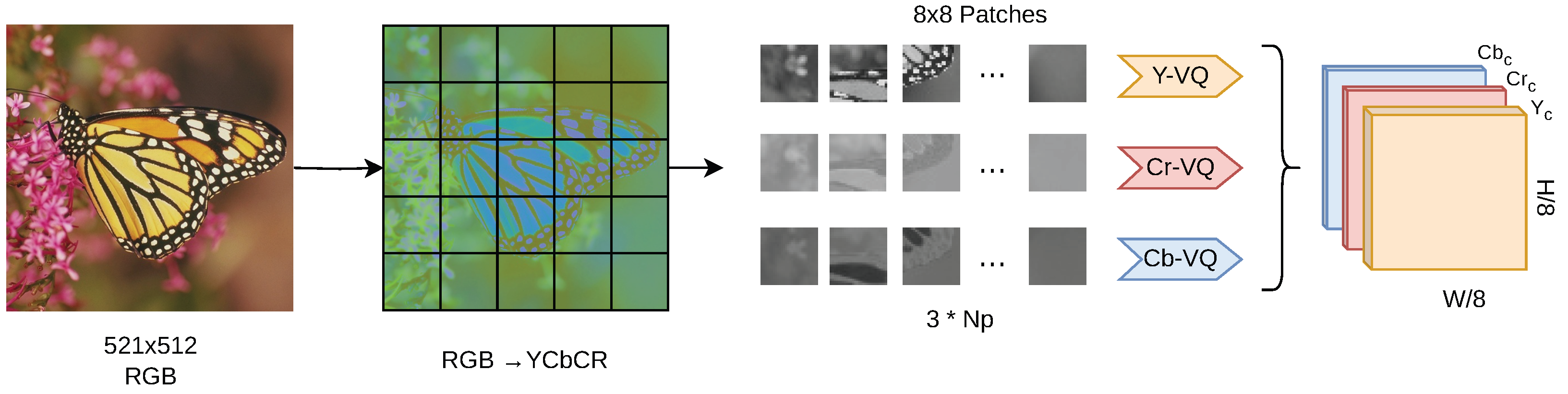
3.1. Latent-Space Encoding

Lossy image compression is a fundamental branch of image processing that addresses the problem of reducing the data required to represent an image by selectively discarding the information that is deemed less relevant for the human perception. Typical lossy compression algorithms encode images in ways that exploit the inherent redundancy, allowing them to be efficiently represented using fewer bits. The first aspect to consider when designing a compression algorithm that can be leveraged for latent-space image synthesis is the convolutional encoder–decoder style of the generative model itself, which can only produce output of fixed size. Conversely, the most popular image compression algorithms, with JPEG on top of all, produce variable-length compressed representations for different images. For this reason, we devise a simple yet effective compression strategy based on VQ techniques, which maintains a constant compressed representation size for each patch by employing predefined codebook mapping input vectors to fixed-length code words, thus ensuring consistent compression regardless of image content. Similar strategies have been popular since the 1980s (see e.g., [13,14]) for their simplicity and overall good performances. In the deep learning era, VQ-like approaches were rediscovered [12], as was the case with other compression techniques [15,16].
Given an RGB image x R w × h × 3 , the model-based compression algorithm produces a latent representation z R w s × h s × c ¯ . The compression algorithm is designed by first converting the image to the YCbCr color space, this separates the image information into its perceptually relevant components, enabling a better use of compression techniques. Then, for each channel from 1 to 3, the image is divided in non-overlapping patches of s × s pixels, with each patch capturing a localized region of the image, preserving both spatial and chromatic information. Then, finally, the core of our compression techniques involves vector quantization applied to each individual patch. Vector quantization replaces each patch with one (or more) representative vector, denoted as codewords, from a fixed-size codebook, thus allowing the whole ( s 2 8 bit) block to be encoded as the index i of the assigned codeword. Clearly, the strategy of the definition of the codebook and the codewords assignment strategy are crucial to set the optimal tradeoff between compression ratio and information preservation; therefore, hereafter, we detail the multiple strategies experimented. The complete compression algorithm is schematized in Figure 1. In Section 4.1, instead, we flesh out all the technical details of the practical implementation of the quantization approaches, together with results on a lossy compression benchmark.

3.1.1. Vector Quantization

Vector quantization [17,18] is a popular technique in the domain of data compression and signal processing. Its fundamental idea is the approximation of the entire data space X with a finite subset of representative vectors C . This process not only reduces the cardinality of the space but also enables a concise and efficient representation by assigning a codeword c i to each element x X of the subset. Conveniently, each entry c i can be uniquely represented by its index i I , with  I { 1 , , | C | } .
Formally, this procedure is described by a quantizer defined by an encoder function E ( x ) and a decoder function D ( i )
q : X C
         x c = q ( x ) = D ( E ( x ) )
The encoder function, E : X I , maps each element of the space into its compact code representation E ( x ) = i I . On the other hand, the decoder function D : I C maps the index i I back to the representative vector c i . The representative vector c i is chosen by definition in order to minimize the distortion with respect to x; hence, the encoder can be defined as
E ( x ) = i x c i 2 2 = min c x c 2 2
From Equation (9), the lossy nature of VQ is clear, since the encoding process implies an approximation error e, or  c i = x + e . For convenience, C is referred to as the c o d e b o o k , and its elements c i as c o d e w o r d s , with i being the code associated to x. For the scope of this work, we focus on fixed-rate quantizers, where each code is represented with the same number of bits; hence, the number of bits required to approximate x with i using a codebook C is b C = l o g 2 ( | C | ) , defined as bitrate of q. When x R n with n > > b C , it makes VQ a very powerful compressor.
Defining an optimal quantizer is not straightforward, as it depends on the desired tradeoff between reconstruction error and compression rate, which is strictly dependent on | C | . In the simple case where X is defined as a finite subset of R n and | C | is fixed beforehand, recalling Equation (9), the formulation for the error introduced by encoding X with q simplifies to
M S E ( q ) = x X x q ( x ) 2 2 = x X x D ( E ( x ) ) 2 2
From this definition, the choice of the optimal quantizer for X reduces to defining the set of vectors c i , which minimizes Equation (10), which are those provided by the k-means algorithm. K-means directly minimizes the MSE by iteratively updating centroids to minimize the sum of squared distances between data points and their assigned centroids. In Section 4.1, we detail the process of defining the optimal quantizer for the problem of image compression, where X is defined as a set of representative image patches.

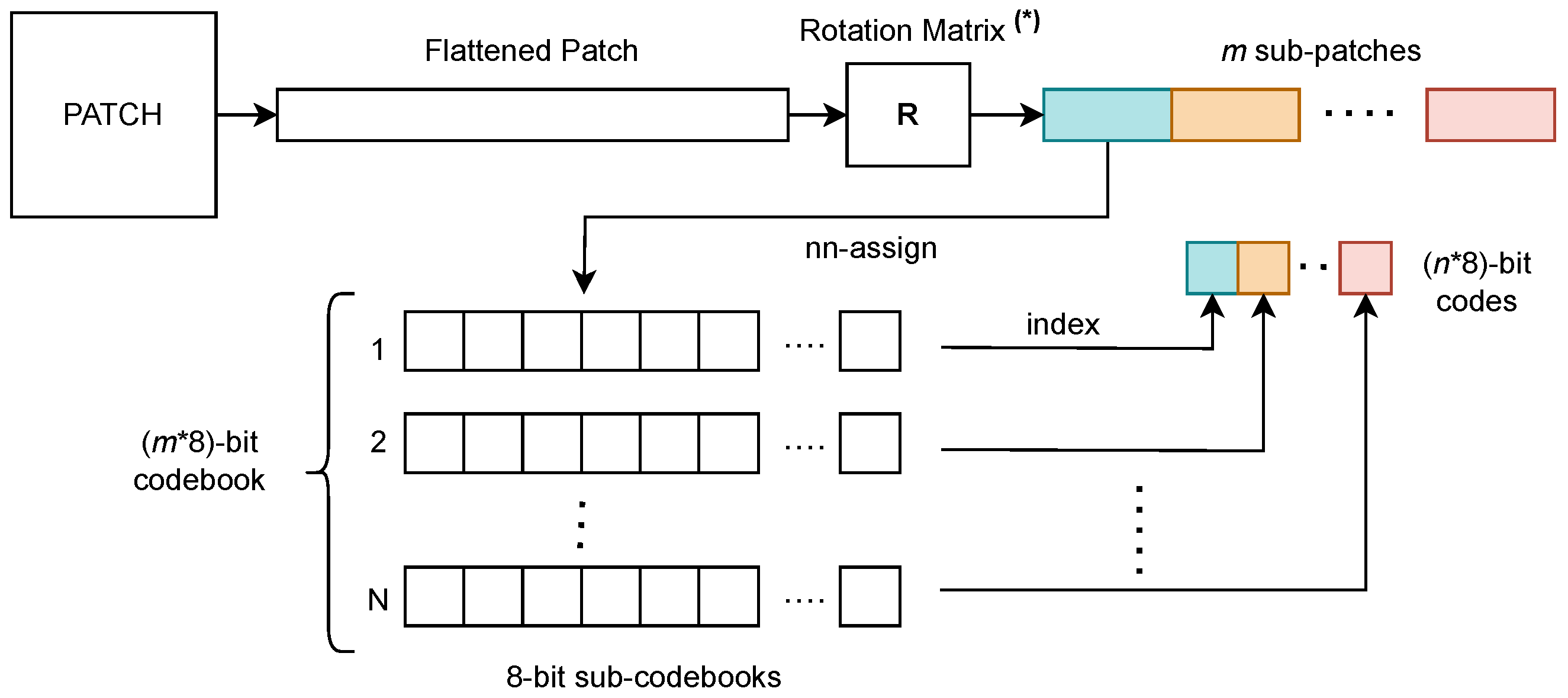
3.1.2. (Optimized) Product Quantization

The base vector quantizer described in Section 3.1.1, while being a powerful tool, implies some major drawbacks. The number of codewords | C | required to represent a code E ( x ) = i using b C bits is proportional to the cardinality of the codebook as | C | = 2 b C . For moderately large x (i.e., an  8 × 8 8-bit grayscale image patch), a reasonably high compression rate of 1 : 16 would imply encoding the block with 512 / 16 = 32 bits, which would lead to a codebook with | C | = 2 32 4 B possible codewords! Clearly, such a large codebook would be hard to obtain and require large memory usage and intense computation cost; hence, more sophisticated quantizers are needed.
Product Quantization (PQ) [19], schematized in Figure 2, is an upgrade in this direction. Instead of processing the input vector x as a whole, it is possible to split it into m subvectors x ( 1 ) , x ( 2 ) , , x ( m ) and consider a subcodebook for each of them. For simplicity, it is common to have subvectors with equal length of n = n m : x ( j ) = ( x m ( j 1 ) + 1 , , x m j ) , where m is a divisor of n. At this point, the quantizer is the Cartesian product of m subquantizers that act on each subvector:
q : X C = C 1 × × C m
           x c = ( c 1 , , c m ) = ( q 1 ( x ( 1 ) ) , , q m ( x ( m ) ) )
Since each subquantizer q j is a separate vector quantizer, defined by its codebook C j , the code for x can be obtained by independently encoding each subvector:
E ( x ) = ( E 1 ( x ( 1 ) ) , , E m ( x ( m ) ) ) = ( i 1 , , i m )
The fundamental difference is that the resulting code ( i 1 , , i m ) is a vector; therefore, the total number of bits required to represent it corresponds to the sum of the bitrates of the subcodebooks. Hence, encoding x with a 32-bit code will require just 4 8-bit codebooks, for a total of only 1024 possible codewords.
Optimized Product Quantization (OPQ) [20] offers further improvement. Instead of directly encoding the vector x as it is, it first applies an orthogonal matrix R (i.e., a change in basis). This operation is particularly useful in our case, as image pixels have correlations between them that are dictated by the structures present in the images subjects. Hence, simply splitting the images at fixed intervals may not be the best course of action, but it may be necessary to first reorder their pixels, so that correlated pixels end up in the same subvector. The problem of finding an optimal quantizer involves finding both the C 1 , , C m codebooks and the matrix R subject to R R T = Id . In [20], the authors derive a nonparametric solution as an alternating minimization scheme, where in one step R is given, and the codebook is learned; in the other, the optimization of the MSE is carried out with respect to R, while the codebook is fixed. The former step can simply be carried out via k-means in the transformed domain. For the latter, considering Equation (10), the problem can be written as
argmin s . t . R R T = Id x X R x R c 2 2 = argmin s . t . R R T = Id R X Y F 2
where, in the last formulation, with a slight abuse of notation, X is the matrix containing the practical data samples from the space, and Y is the reconstruction of X in the transformed domain according to the current codewords estimates (i.e., Y = D ( E ( X ) ) ). This problem is known as Generalized Procrustes Alignment [21] and has a closed-form solution in R = V U T , with V and U being the orthogonal matrices of the Singular Value Decomposition of X Y T .

3.1.3. Residual Quantization

A different strategy to improve VQ is represented by additive quantization [22]. In this case, the quantizer q can be seen as the sum of a set of quantizers { q j } j = 1 m . Each of these quantizers maps the vector x into its own codebook C j :
q : X C
x c = j = 1 m c j = j = 1 m q j ( x )
Similarly to PQ, the code assigned to x is a vector in R m , and the bitrate of the encoding corresponds to the sum of the bitrates of the subcodes. Unlike in PQ, here, the centroids are vectors with the same length as x and not just a fraction of it.
Residual Quantization (RQ) [23] is a specific example of additive quantization. The idea is to give a hierarchy to the quantizers q j . The first one, q 1 , is learned normally without any additional information. The second one, instead, wants to be the optimal quantizer for the vector x q 1 ( x ) , i.e., the residual between x and its quantization. In general, for  j 2 , q j is meant to quantize the vector x s = 1 j 1 q s ( x ) , which effectively places this strategy under the additive quantization umbrella. While RQ demonstrated superior performance in minimizing reconstruction errors, as shown in Section 4.1, it exhibits a fundamental limitation. Specifically, it allows for the possibility of multiple valid encodings for a single data point, which undermines the core principles of the generative model training procedure.

3.2. Latent-Space Diffusion Models

The lossy compression algorithm defines an encoding function E which maps an image x to a latent representation z R w s × h s × c ¯ . Ideally, redefining the training objective of the generative model to operate in the new latent space should be straightforward:
min θ ϵ ϵ θ ( z t , t ) 2 2 z t = E ( x t )
This approach has been shown to be valid in the case of a latent space defined by a deep autoencoder [6,12]. However, when relying on the shallow latent space defined by the proposed compression algorithm, we observed the impossibility of learning anything useful. The causes of this limitation can be traced back to the definition of the encoding algorithm using VQ (and its other embodiments),  especially in the definition of the codewords using k-means, as defined in Equation (10). Effectively, the encoding of an image patch with the assigned code i I imposes a bi-univocal correspondence with the set of positive integers, which implies an inherent total ordering of the codewords c 1 , , c | I | . The imposed ordering, which by the nature of k-means is fundamentally random, is not reflected in an ordering of the R n space where codewords are defined; hence, the addition of Gaussian noise to i will result in the random assignment of a new codeword c i + N ( 0 , 1 ) , while ideally the additive noise should lead to a codeword c j c i + N ( 0 , 1 ) . The above can be intuitively appreciated by observing the effect of a constant addition on an encoded image in Figure 3b.
A useful interpretation is to consider the codewords as a finite and discrete set of categorical data, which brings us to the domain of categorical diffusion models, previously introduced in Section 2.2. Recent works on discrete-state diffusion models [24,25,26,27,28] mainly propose to redefine the forward diffusion process by relying on a transition matrix which defines the probabilities of moving from one state to another. An interesting result of [24] is that we can imitate a continuous-space diffusion model by defining the discrete diffusion process in a way that will transit with higher probability to similar states, introducing an ordinal bias. Along this line, we show that the careful choice of an optimal ordering on C can be leveraged to approximate as a continuous process virtually with no additional work.

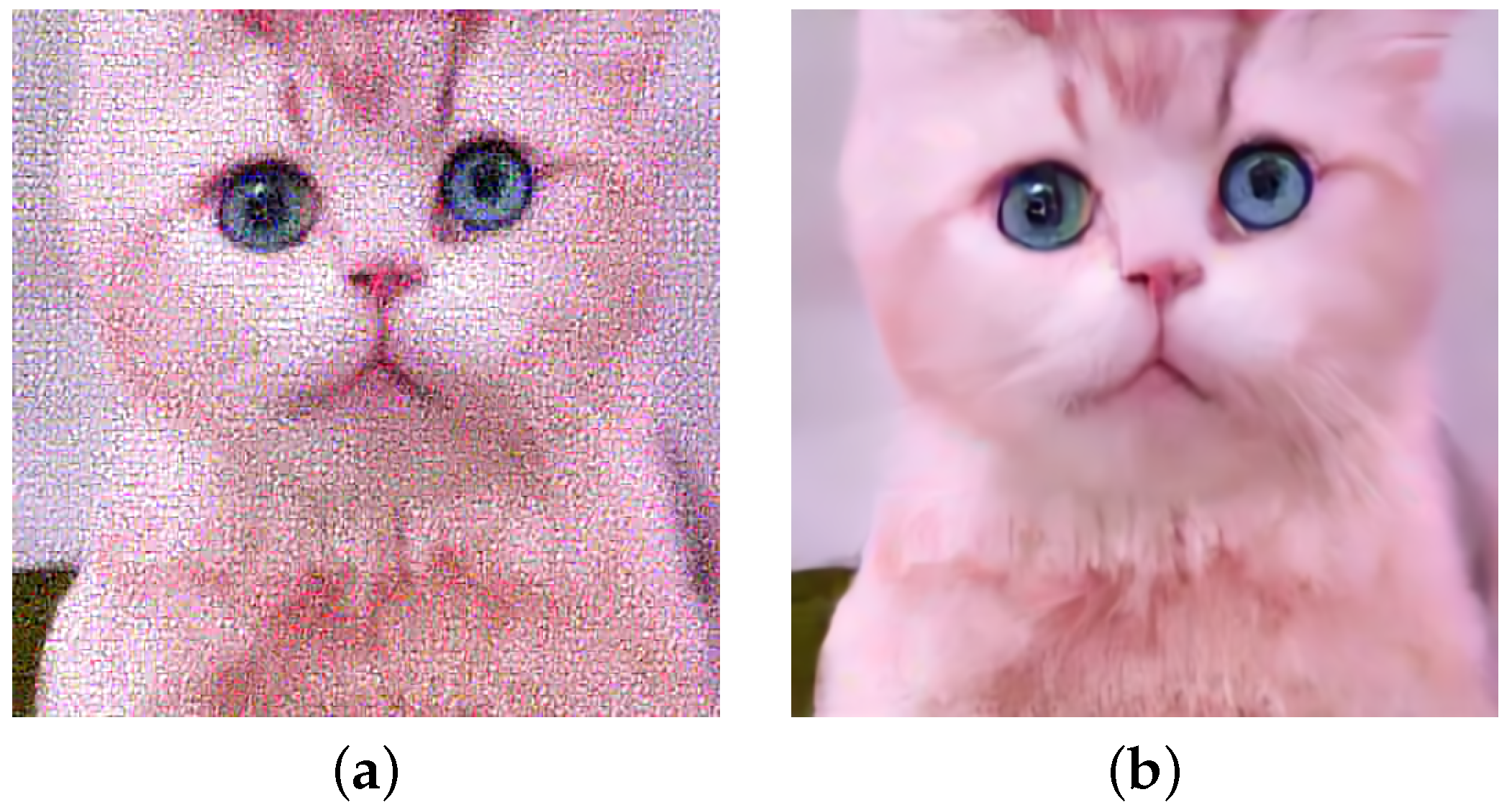
3.2.1. Enforcing Pseudo-Ordinality

In principle, we are interested in an ordering of the code space I which satisfies an ordinality property on the codewords space C in R n :
c i + 1 c i 2 <   c i + j c i 2 i { 1 , , | C | 1 } , j { 2 , , | C | i }
c i 1 c i 2 >   c i j c i 2 i { 2 , , | C | } , j { 2 , , i 1 }
In this way, we can enforce that the addition of noise leads to a transition to a code that is similar to the source code in proportion to the level of noise added. Clearly, with  n > 1 , and in the absence of additional constraints on the codebook’s definition, the existence of a suitable mapping R n R that defines I cannot be guaranteed, and in most cases simply will not exist. More specifically, if we look at the codewords as vectors in R n , there could be an arbitrary number of values j which satisfy the right part of the expression in Equations (18) and (19), i.e., there could be multiple elements of C , identified by different indexes j, which are equidistant from c i . Therefore, we propose a relaxation of the desired property by imposing an ordering along the direction which maximizes the correlation between the elements of C . This approach is borrowed from the technique of Principal Components Analysis (PCA) [29], widely used in the context of dimensionality reduction. Given a generic VQ codebook C R n , its principal component v 0 R n can be conveniently computed as the eigenvector of the covariance matrix of C corresponding to its largest eigenvalue. The projection of c i C along the principal component is hence computed as c i 0 = c i v 0 , which also represents a mapping R n R . We assign each element of C to an index i { 1 , , | C | } such that c i 0 > c i + 1 0 , or in simpler terms, as the indices that sort the vectors through their principal components. This approach does not strictly satisfy the properties in Equations (18) and (19), nor does it assures to maximize the correlation between adjacent pairs, but it is guaranteed to be the best possible achievable approximation with a linear transformation. The latter claim is secured by the fact that PCA, in its linear version, is the linear component reduction technique that best preserves explained variance. The additive noise in the diffusion process then causes a displacement along the maximum variance dimension, which in a categorical framework implies moving towards a highly correlated latent state, which resembles the continuous diffusion process. Figure 4 provides a powerful intuition of the achievement.

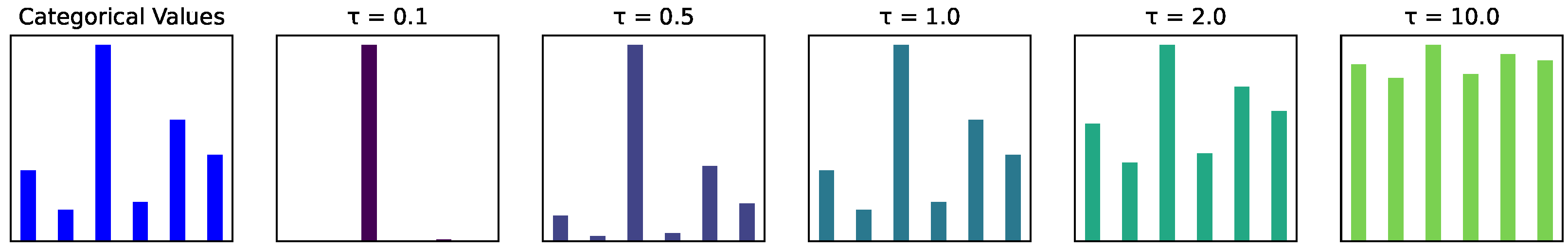
3.2.2. Categorical Posterior Distribution

Despite the promising results in training the DDPM in latent space, thanks to the approximation introduced above by optimizing for the training objective of Equation (4), the sample quality of the decoded images As an additional enhancement, we revise the formulation of the inverse process to better align with the inherent characteristics of VQ-encoded images. Building upon the training objective presented in Equation (5), learning the reverse process within the latent space by targeting the uncorrupted sample z R w s × h s × c ¯ implies predicting the index i corresponding to the suitable codebook entry c i C j for each codebook j ( 1 , , c ¯ ) at each spatial location. Instead of directly regressing the value of c i , we propose an alternative strategy, wherein the inverse process targets a categorical distribution for each codebook entry across all utilized codebooks. Assuming that all codebooks contain the same number of entries, the output for the reverse process can be parametrized as z ^ R w s × h s × c ¯ × | C | so that the recovered sample z ˜ could be obtained by sampling the corresponding categorical distribution at each spatial location. The forward diffusion process instead is kept unchanged, with  z t being defined by introducing noise to z in the index space.
Since the sampling operation is nondifferentiable, in the training phase, we leverage the Gumbel-Softmax trick [30] to approximate the sampling of the categorical distribution; this is achieved by perturbing the logits z ^ j for each category with Gumbel-distributed noise G i G u m b e l ( 0 , 1 ) , and then approximating the one-hot vector representing the categorical choice by applying the Softmax function to the perturbed logits. Mathematically, this can be expressed as
z ¯ j = s o f t m a x z ^ j + G τ j = 1 , , c ¯ G G u m b e l ( 0 , Id )
The hyperparameter τ is a temperature parameter which increases the entropy of the distribution; hence, for τ 0 , it approaches the a r g m a x function, and for τ , it approaches the uniform distribution, as depicted in Figure 4. Notably, this approximation allows us to explicitly sample from the codebook distribution instead of the index distribution. Consequently, we can decode the predicted codewords in a fully differentiable manner, as demonstrated by the equation
c ˜ = [ z ¯ 1 C 1 , , z ¯ c ¯ C c ¯ ]
and the decoded image x ˜ can be recovered from c ˜ depending on the utilized VQ specific (the complete procedure is schematized in Algorithm 1). By leveraging this formulation, we could compute the training objective in image space as in Equation (5), while still performing the generation and the gradient computation in the latent space. It is worth noticing that, in this way, the latent codes for z are never elicited in the training objective.
Algorithm 1 Differentiable decoding denoised sample
Require: noisy sample z t , time step t
Ensure: denoised sampled in image space x ˜ 0
     predicted _ codewords = empty ( )
     z ^ 0 nn ( z t , t )                      ▹ z ^ 0 R w s × h s × c ¯ × | C |
    for each channel c ( 1 , , c ¯ )  do
        for all i,j do
             z ¯ 0 [ i , j , c ] = gumbel _ softmax ( z ^ 0 [ i , j , c ] )
             c ˜ z ^ 0 [ i , j , c ] C c
             predicted _ codewords [ i , j , c ] c ˜
        end for
    end for
    return vq _ decode ( prediced _ codewords )
In order to sample from the trained model, the only distinction from the standard parameterization of the reverse process in the latent space is that deriving the next sample z t 1 requires obtaining z ˜ by sampling from the categorical distributions derived from z ^ , which is achieved by the assigned codebook index from the corresponding categorical distribution, this is schematized in Algorithm 2. It is worth noticing that simply taking the index with the largest logit (argmax function) corresponds to using the mode of the categorical distribution, which contrasts with the definition of the inverse process.
Algorithm 2 Sampling
Require: noisy sample z t , time step t
Ensure:  z ˜ t 1
     z ^ 0 nn ( z t , t )
    for all i,j do
         z ˜ 0 [ i , j ] sample ( z ^ [ i , j ] )
    end for
     z ˜ t 1 reverse ( z ˜ 0 , t 1 ) ▹ implementation of the reverse process parametrized by z 0
    return  z ˜ t 1

4. Experiments and Evaluation

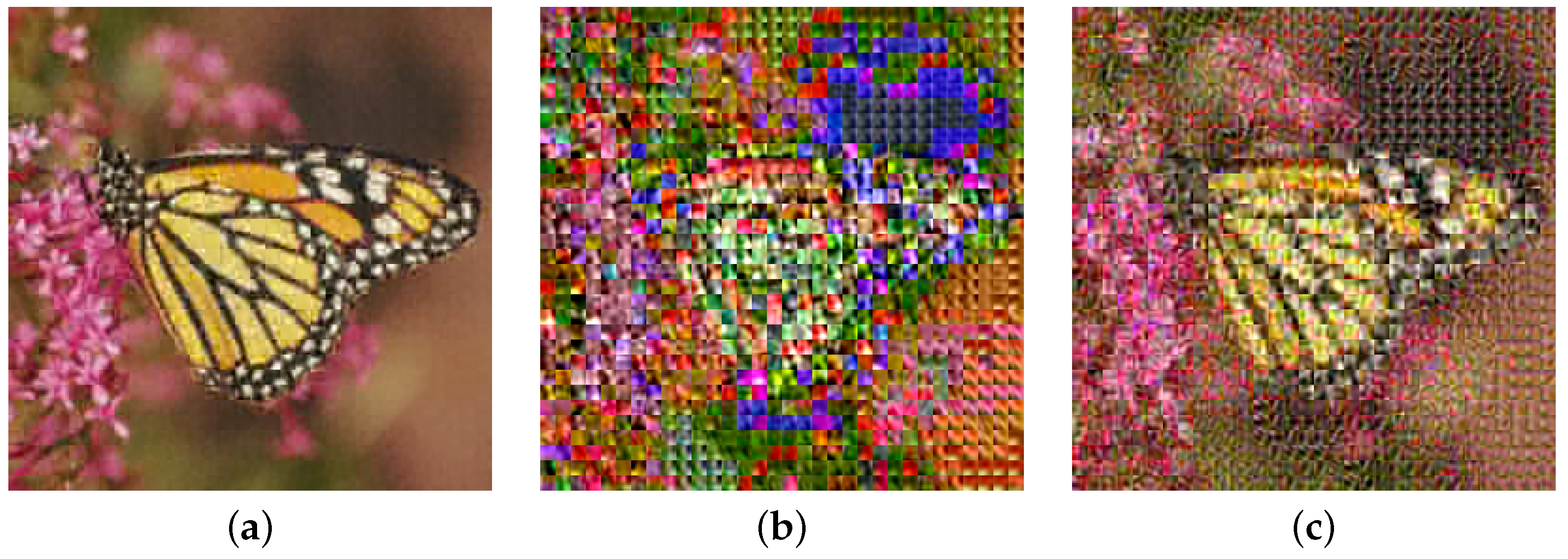
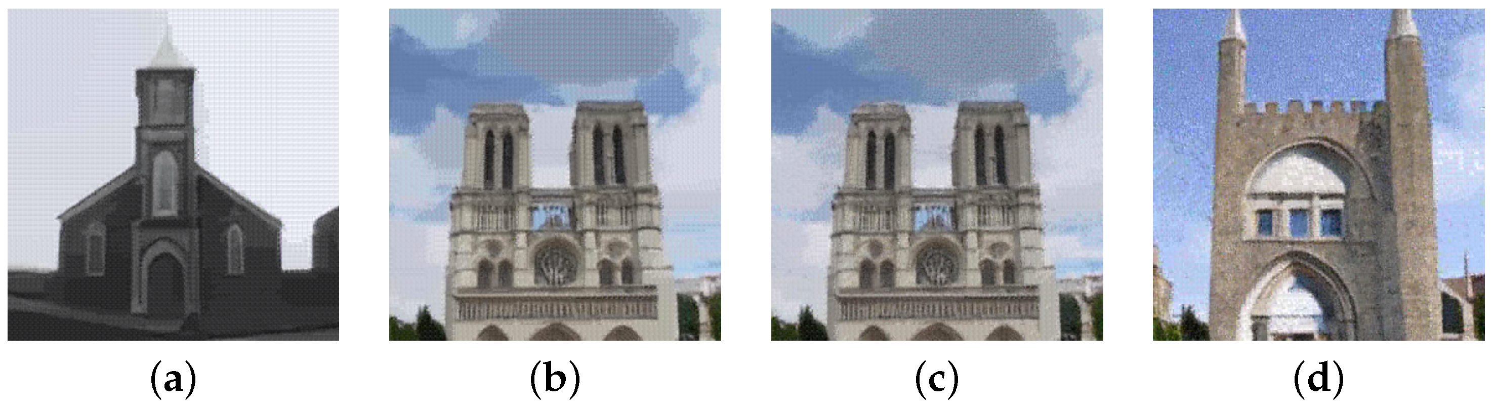
4.1. Image Compression

In this section, we detail the implementation detail of the VQ-based image encoding algorithm introduced in Section 3.1 and provide the qualitative analysis that led to picking the exact configuration used to train the generative models.
The size of the patch is fixed to s = 8 for all models, and the VQ training set is defined by extracting all the possible patches from the 18 high-quality images of the McM dataset [31], which are augmented to 36 by vertically flipping each one, leading to just over 8.6 million patches. Once a VQ method (among VQ, PQ/OPQ, and RQ) is picked, a distinct VQ encoder is trained for each channel in YCbCr space by leveraging the implementations of the FAISS library [32] for maximum efficiency. Each channel can be encoded with a different bitrate; hence, we use the notation {VQ}-{ Y b - C r b - C b b } to uniquely identify the used combination of VQ type and assigned bitrates.
Each method is tested on three standard images of size 512 × 512 , which have been used in the image compression literature for decades (https://sipi.usc.edu/database/, accessed on 24 October 2023) [33]. The performance is evaluated with two different quality measures. The Peak Signal-to-Noise Ratio (PSNR) is defined as
P S N R ( x 1 , x 2 ) = 20 l o g 10 255 M S E ( x 1 , x 2 ) M S E ( x 1 , x 2 ) = 1 h w i = 1 h j = 1 w x 1 ( i , j ) x 2 ( i , j ) 2 2
and takes values on all the real lines, where the smaller the number, the worse the quality of the image. The other is the Structural SIMilarity index (SSIM), which can be computed as
S S I M ( x 1 , x 2 ) = ( 2 μ x 1 μ x 2 + c 1 ) ( 2 σ x 1 x 2 + c 2 ) ( μ x 1 2 + μ x 2 2 + c 1 ) ( σ x 1 2 + σ x 2 2 + c 2 )
where, for i = 1 , 2 , μ x i is the mean of x i , σ x i is its standard deviation, and σ x 1 x 2 is the covariance between the two images. The constants c 1 and c 2 are constants placed in order to avoid numerical issues. The SSIM of an image takes values in the interval [ 0 , 1 ] , where a score of 0 implies an heavy dissimilarity between the images, while a score of 1 means the contrary. We also report the compression ratio, which, since the patch size is fixed, can be conveniently computed as
R ( q ) = 3 8 s 2 Y b + C r b + C b b
where Y b , C r b , and C b b represent the number of bits needed to represented the pixel value for the respective channel.
The results reported in Table 1 are in line with what was expected: baseline VQ severely underperforms (especially in terms of SSIM), and increasing the bitrate for the luminance channel yields far better results, while still achieving a high compression ratio. The absolute best results are obtained with RQ, which, however, turned out to be unsuitable for our application because of the commutative propriety of the sum, also being computationally inefficient for the sequential nature of the encoding. In addition, basic PQ really does not make much sense, because it produces highly redundant codebooks. For the above reasons, we chose to proceed with OPQ-32-8-8. We also report the results obtained on the same benchmark by two configurations of the pretrained VAE used in [6]. It is imperative to acknowledge that although the metrics under evaluation may not explicitly highlight this phenomenon, deep encoding tends to yield markedly more visually appealing images. This phenomenon can likely be attributed to the fact that shallow encoding introduces high-frequency and blocky artifacts, which are very noticeable to the human visual system, while deep encoding produces high-level errors that are not obvious at a glance unless a side-by-side comparison is made.

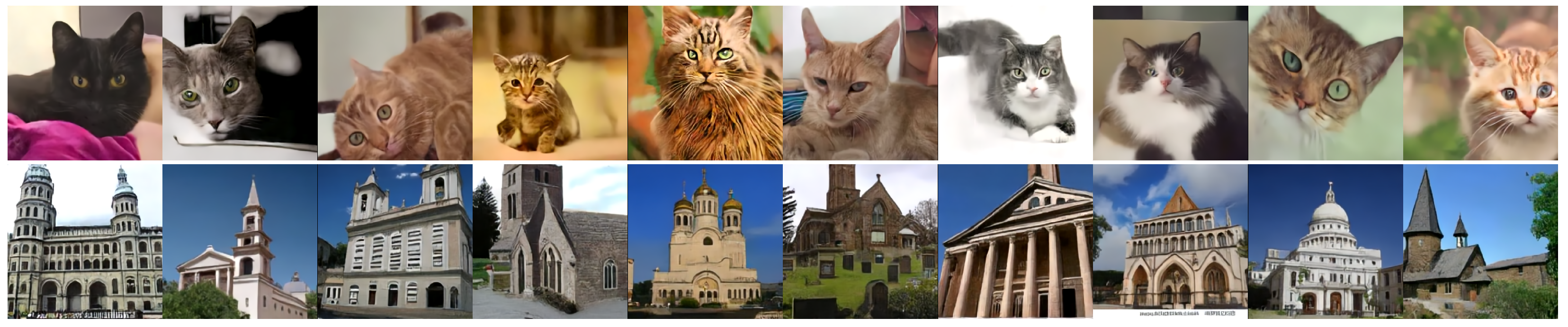
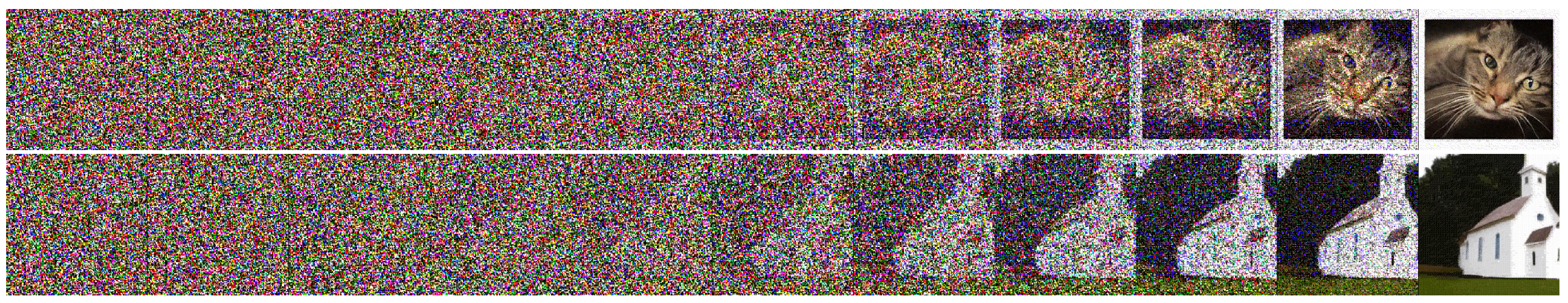
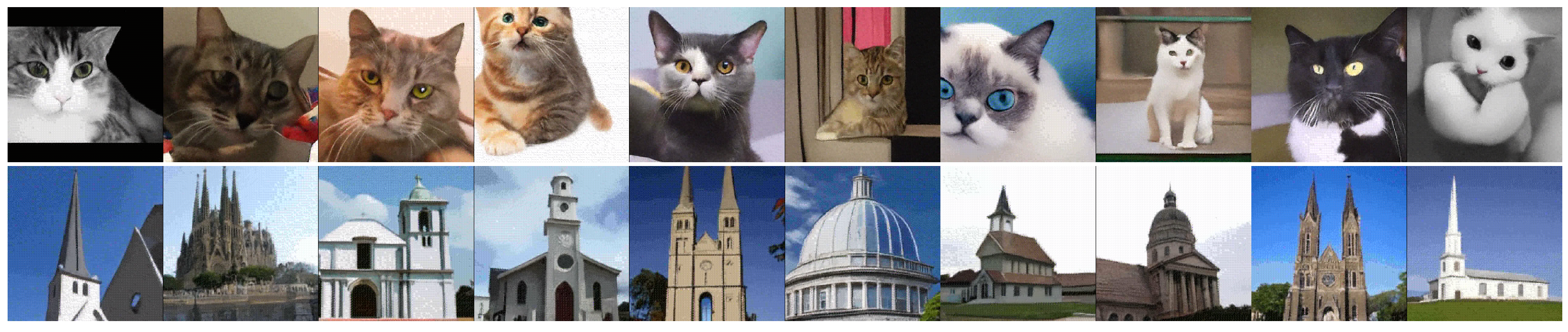
4.2. Image Generation

In this section, we provide an experimental evaluation of the proposed approach in a popular benchmark for unconditional image generation. As introduced in Section 2.1, the definition of a metric for evaluating generative models is still an open problem; hence, for the remainder of this section, we opted to stick with the FID score, which, to date, is the most popular metric in the literature.

4.2.1. Experimental Setup

We assess the generative performances in a single-class unconditional scenario on two subsets of the LSUN dataset [34] which are extremely popular in this context: the cat subset and the church one. The first is a large dataset of over 1.6 million images of cats acquired from a wide variety of sources. This is a very complicated dataset due to the extreme variability in the appearance and composition of the images, caused in part by the nature of the subject. In contrast, the dataset of churches is smaller with only 125 thousand images, and it is considerably easier to handle because of the chromatic and geometric regularity of the buildings represented. All the experiments are conducted with an image resolution before compression of 512 × 512 , which means a latent representation of 64 × 64 × 6 using the OPQ-{32-8-8} encoding.
We fix a common setup for all the experiments: the denoiser model is defined as a U-Net model with four down/up sampling stages and attention only at the bottleneck level in order to reduce the memory footprint. In total, the model has around 50 million parameters, which is a small number if compared with what is commonly used. We base our experimental setup on the Pytorch implementation by Phil Wang of the original DDPM paper, with the addition of Min-SNR weighting [35], which penalizes the loss terms proportionally to the inverse of the magnitude of the noise added al timestep t. In this way, the model is discouraged from focusing on minor details and self-conditioning [36], which conditions the denoising process based on the previous estimate of the recovered sample x ˜ 0 . All the evaluated models are trained for 1 million steps with a batch size of 64 on 2 Nvidia v100 GPUs, which takes around 10 days. This represents an extremely tight computational budget for this kind of application. In comparison, in the original DDPM, a U-Net configuration with either 114 or 256 million parameters (approximately 2–5 times larger than ours) is leveraged and trained for the equivalent of over 100 v100 days, which is over 10 times our computational budget. An additional difference is that, thanks to the efficiency of the proposed encoding, we are able to generate samples of size 512 × 512 , which after encoding with the chosen setup (OPQ-{32-8-8}) corresponds to latent codes of size 64 × 64 × 6 . Other existing methods, such as the original DDPM [1], typically use samples of size 256 × 256 , i.e., 1 4 of the size of our decoded samples. The results, expressed in terms of FID score, are shown in Table 2.

4.2.2. Continuous-Style Diffusion Model

We begin this evaluation by analyzing the case in which the forward and backward processes are kept unchanged compared with the continuous case. Hence, we optimize for the objective in Equation (4) while leveraging the codeword-to-index assignment introduced in Section 3.2.1. As anticipated, the generative process is able to infer and reproduce the high-level structure of real images and model the textures and details. Where this approach fails is in the last steps of the inverse process, since the ambiguity introduced by the approximation to the continuum seems to limit the overall definition of the finest details in the image, resulting in an extremely noisy generated image.
As an impromptu solution, we opted to train a trimming model to improve the quality of the generated image x ˜ = D ( z ˜ ) after it has been decoded to RGB space. The refiner is based on the same U-Net architecture with a smaller configuration with only 1.7 M parameters, and it is trained in a fully supervised fashion by synthetically generating noisy images x n by slightly corrupting their encoded representation, x n = D ( E ( x ) + γ ) , where γ is scaled-down Gaussian noise. The objective function for the refiner is a combination of L 1 and SSIM losses, which easily achieves a PSNR of over 30 on both datasets. The clear downside of this solution is the necessity of training a custom refiner for each dataset and the increased cost of generating new images. In Figure 5 the effect of the refiner model can be appreciated, while in Figure 6 a batch of refined generated samples are reported for qualitative evaluation.

4.2.3. Categorical Reverse Process

Comparatively, we evaluate the performance obtained with the formulation introduced in Section 3.2.2 for the definition of the reverse process. At training time, we leverage the objective function of Equation (5) with the differentiable decoding of x ˜ 0 derived in Equation (21). We found out that it is preferable to add a second term to the loss in order to condition the prediction of z 0 codes based on those assigned by the VQ encoding, which are otherwise not explicitly in the derivation of x ˜ 0 .
The complete training objective used is
L c a t ( θ ) = | | x 0 x ˜ 0 θ | | 2 2 + | | ϵ ϵ z θ | | 2 2 ϵ z θ = ( a t z t z ˜ 0 θ ) / b t ,
where
  • ϵ z θ is the derivation for the predicted noise in latent space, obtained from the prediction for the uncorrupted image z ˜ 0 θ sampled from z ^ 0 using the Gumbel-Softmax trick;
  • a t and b t are time-dependent constants values that are derived from the detailed definition of the diffusion process in [1], the details of which we omit for simplicity;
  • The θ superscript is added to indicate values that are a function of model parameters.
In this configuration, satisfactory results are obtained without resorting to the refiner model, as it can be appreciated in Figure 7 and Figure 8. One interesting thing to study is the introduction of a temperature smoothing at inference time in the generative process (i.e., deriving z t 1 given z t ). Since z t 1 is obtained from the current estimate for z ˜ 0 , we can introduce a temperature factor γ in the sampling of z ˜ 0 from z ^ 0
z ˜ 0 s o f t m a x z ^ 0 / γ
The effect of the introduction of γ can be qualitatively appreciated in Figure 9. In particular, for γ 0 , the sampling operation corresponds to the a r g m a x function and essentially defines the mode of the categorical distribution, while for larger values of γ , the distribution shifts towards a uniform distribution.

4.3. Discussion

In this study, we conducted comprehensive experiments to evaluate the performance of our proposed image compression and generation techniques. On the compression side, the results demonstrate the effectiveness of the VQ-based image encoding algorithm, specifically, the OPQ-{32-8-8} configuration emerged as the most promising, striking a balance between compression ratio and image quality. Regarding the image generation task, it is important to stress that competing with state-of-the-art generative models is beyond the scope of this work and would be Utopian given the possibilities of our academic budget; hence, the results provided are primarily intended to demonstrate the applicability of the proposed methodology. Nevertheless, the results obtained are compelling: the continuous-style model served to demonstrate the goodness of the proposed approximation for the continuous representation of discrete space, and with the addition of the refiner, it is able to consistently produce visually appealing images. The categorical parameterization further improves the fit of the inverse process to the discrete case and produces images with greater visual appeal, mitigating issues of high-frequency artifacts and eliminating the need for a refiner model. The introduction of temperature smoothing during inference showcased its ability to control the level of stochasticity in the generative process, offering flexibility in the tradeoff between image quality and diversity.

5. Conclusions

In conclusion, with the proposed approach, although not without problems and limitations, convincing results have been achieved in the image generation task. The idea of approximating to the continuous state by rearranging the discrete space proved to be valid, although the way it was defined is not entirely satisfactory and requires refinement of the generated images. The categorical parameterization of the inverse model has partially improved this aspect but with some flaws remaining, such as the oversimplification of details in the generated images, which can be partially modulated by acting on the temperature parameter of the distribution. Furthermore, the proposed image compression scheme, although being a well-known and long-established concept, has proven to be an excellent use case for the study of generative models for categorical data. Therefore, the experimental concepts could be applied to other applications, such as language generation or other token-based discrete structures where the variables are not strictly ordinal.

Author Contributions

Conceptualization, C.S. and D.P.; methodology, D.P.; software, C.S.; validation, G.F.; formal analysis, G.F. and D.P.; investigation, D.P.; data curation, C.S.; writing—original draft preparation, C.S.; writing—review and editing, C.S., D.P., G.F. and M.P.; supervision, M.P. All authors have read and agreed to the published version of the manuscript.

Funding

This research received no external funding.

Data Availability Statement

The implementation will be made publicly available at: https://github.com/cscribano/model-based-ldm, accessed on 24 October 2023.

Acknowledgments

This work was also supported by the Gruppo Nazionale per il Calcolo Scientifico (GNCS-INdAM). The publication was created with the co-financing of the European Union-FSE-REACT-EU, PON Research and Innovation 2014-2020 DM1062/2021.

Conflicts of Interest

The authors declare no conflict of interest.

Glossary of Mathematical Notation

w, hWidth and height of the image
cNumber of channels
E Image encoding function to latent space
D Decoding function from latent space
zEncoded image in latent space
x ˜ , z ˜ Generated image, generated latent representation.
c ¯ Number of channels of the latent representation
sPatch size
qquantizer
EVQ Encoder
DVQ Decoder
nLength of the vector to be encoded
mNumber of subquantizers in PQ and RQ
ROPQ Rotation matrix
C Generic VQ Codebook
cGeneric codebook element
iIndex of the codebook entry c i
I Set of the indices i
c i 0 Principal component on the i-th codebook entry
XSet of R n vectors to be approximated by q
b C Number of bits used to encode a vector with C (bitrate).

References

  1. Ho, J.; Jain, A.; Abbeel, P. Denoising diffusion probabilistic models. Adv. Neural Inf. Process. Syst. 2020, 33, 6840–6851. [Google Scholar]
  2. Dhariwal, P.; Nichol, A. Diffusion models beat gans on image synthesis. Adv. Neural Inf. Process. Syst. 2021, 34, 8780–8794. [Google Scholar]
  3. Esser, P.; Rombach, R.; Ommer, B. Taming Transformers for High-Resolution Image Synthesis. In Proceedings of the 2021 IEEE/CVF Conference on Computer Vision and Pattern Recognition, Nashville, TN, USA, 20–25 June 2021. [Google Scholar]
  4. Ramesh, A.; Pavlov, M.; Goh, G.; Gray, S.; Voss, C.; Radford, A.; Chen, M.; Sutskever, I. Zero-shot text-to-image generation. In Proceedings of the International Conference on Machine Learning. PMLR, Online, 18–24 July 2021; pp. 8821–8831. [Google Scholar]
  5. Ding, M.; Yang, Z.; Hong, W.; Zheng, W.; Zhou, C.; Yin, D.; Lin, J.; Zou, X.; Shao, Z.; Yang, H.; et al. CogView: Mastering Text-to-Image Generation via Transformers. In Proceedings of the Advances in Neural Information Processing Systems, Online, 6–14 December 2021; Ranzato, M., Beygelzimer, A., Dauphin, Y., Liang, P., Vaughan, J.W., Eds.; Curran Associates, Inc.: Red Hook, NY, USA, 2021; Volume 34, pp. 19822–19835. [Google Scholar]
  6. Rombach, R.; Blattmann, A.; Lorenz, D.; Esser, P.; Ommer, B. High-resolution image synthesis with latent diffusion models. In Proceedings of the IEEE/CVF Conference on Computer Vision and Pattern Recognition, New Orleans, LA, USA, 18–24 June 2022; pp. 10684–10695. [Google Scholar]
  7. Salimans, T.; Goodfellow, I.; Zaremba, W.; Cheung, V.; Radford, A.; Chen, X. Improved techniques for training gans. Adv. Neural Inf. Process. Syst. 2016, 29, 2234–2242. [Google Scholar]
  8. Deng, J.; Dong, W.; Socher, R.; Li, L.J.; Li, K.; Fei-Fei, L. Imagenet: A large-scale hierarchical image database. In Proceedings of the 2009 IEEE Conference on Computer Vision and Pattern Recognition, Miami, FL, USA, 20–25 June 2009; pp. 248–255. [Google Scholar]
  9. Heusel, M.; Ramsauer, H.; Unterthiner, T.; Nessler, B.; Hochreiter, S. Gans trained by a two time-scale update rule converge to a local nash equilibrium. Adv. Neural Inf. Process. Syst. 2017, 30, 6626–6637. [Google Scholar]
  10. Parmar, G.; Zhang, R.; Zhu, J.Y. On Aliased Resizing and Surprising Subtleties in GAN Evaluation. In Proceedings of the IEEE/CVF Conference on Computer Vision and Pattern Recognition, New Orleans, LA, USA, 18–24 June 2022. [Google Scholar]
  11. Kuznetsova, A.; Rom, H.; Alldrin, N.; Uijlings, J.; Krasin, I.; Pont-Tuset, J.; Kamali, S.; Popov, S.; Malloci, M.; Kolesnikov, A.; et al. The open images dataset v4: Unified image classification, object detection, and visual relationship detection at scale. Int. J. Comput. Vis. 2020, 128, 1956–1981. [Google Scholar] [CrossRef]
  12. Van Den Oord, A.; Vinyals, O. Neural discrete representation learning. Adv. Neural Inf. Process. Syst. 2017, 30, 6306–6315. [Google Scholar]
  13. Goldberg, M.; Boucher, P.; Shlien, S. Image Compression Using Adaptive Vector Quantization. IEEE Trans. Commun. 1986, 34, 180–187. [Google Scholar] [CrossRef]
  14. Nasrabadi, N.; King, R. Image coding using vector quantization: A review. IEEE Trans. Commun. 1988, 36, 957–971. [Google Scholar] [CrossRef]
  15. Scribano, C.; Franchini, G.; Prato, M.; Bertogna, M. DCT-Former: Efficient Self-Attention with Discrete Cosine Transform. J. Sci. Comput. 2023, 94, 67. [Google Scholar] [CrossRef]
  16. Garg, I.; Chowdhury, S.S.; Roy, K. DCT-SNN: Using DCT To Distribute Spatial Information Over Time for Low-Latency Spiking Neural Networks. In Proceedings of the IEEE/CVF International Conference on Computer Vision (ICCV), Montreal, BC, Canada, 11–17 October 2021; pp. 4671–4680. [Google Scholar]
  17. Gray, R. Vector quantization. IEEE Assp Mag. 1984, 1, 4–29. [Google Scholar] [CrossRef]
  18. Gray, R.; Neuhoff, D. Quantization. IEEE Trans. Inf. Theory 1998, 44, 2325–2383. [Google Scholar] [CrossRef]
  19. Jegou, H.; Douze, M.; Schmid, C. Product quantization for nearest neighbor search. IEEE Trans. Pattern Anal. Mach. Intell. 2010, 33, 117–128. [Google Scholar] [CrossRef] [PubMed]
  20. Ge, T.; He, K.; Ke, Q.; Sun, J. Optimized Product Quantization. IEEE Trans. Pattern Anal. Mach. Intell. 2014, 36, 744–755. [Google Scholar] [CrossRef] [PubMed]
  21. Schönemann, P.H. A generalized solution of the orthogonal procrustes problem. Psychometrika 1966, 31, 1–10. [Google Scholar] [CrossRef]
  22. Babenko, A.; Lempitsky, V. Additive quantization for extreme vector compression. In Proceedings of the IEEE Conference on Computer Vision and Pattern Recognition, Columbus, OH, USA, 23–28 June 2014; pp. 931–938. [Google Scholar]
  23. Chen, Y.; Guan, T.; Wang, C. Approximate Nearest Neighbor Search by Residual Vector Quantization. Sensors 2010, 10, 11259–11273. [Google Scholar] [CrossRef]
  24. Austin, J.; Johnson, D.D.; Ho, J.; Tarlow, D.; Van Den Berg, R. Structured denoising diffusion models in discrete state-spaces. Adv. Neural Inf. Process. Syst. 2021, 34, 17981–17993. [Google Scholar]
  25. Hoogeboom, E.; Nielsen, D.; Jaini, P.; Forré, P.; Welling, M. Argmax flows and multinomial diffusion: Learning categorical distributions. Adv. Neural Inf. Process. Syst. 2021, 34, 12454–12465. [Google Scholar]
  26. Campbell, A.; Benton, J.; De Bortoli, V.; Rainforth, T.; Deligiannidis, G.; Doucet, A. A continuous time framework for discrete denoising models. Adv. Neural Inf. Process. Syst. 2022, 35, 28266–28279. [Google Scholar]
  27. Vahdat, A.; Kreis, K.; Kautz, J. Score-based generative modeling in latent space. arXiv 2021, arXiv:2106.05931. [Google Scholar]
  28. Tang, Z.; Gu, S.; Bao, J.; Chen, D.; Wen, F. Improved vector quantized diffusion models. arXiv 2022, arXiv:2205.16007. [Google Scholar]
  29. Jolliffe, I.T.; Cadima, J. Principal component analysis: A review and recent developments. Philos. Trans. R. Soc. A Math. Phys. Eng. Sci. 2016, 374, 20150202. [Google Scholar] [CrossRef] [PubMed]
  30. Jang, E.; Gu, S.; Poole, B. Categorical reparameterization with gumbel-softmax. arXiv 2016, arXiv:1611.01144. [Google Scholar]
  31. Zhang, L.; Wu, X.; Buades, A.; Li, X. Color demosaicking by local directional interpolation and nonlocal adaptive thresholding. J. Electron. Imaging 2011, 20, 023016. [Google Scholar]
  32. Johnson, J.; Douze, M.; Jégou, H. Billion-scale similarity search with GPUs. IEEE Trans. Big Data 2019, 7, 535–547. [Google Scholar] [CrossRef]
  33. Roberts, L. Picture coding using pseudo-random noise. IRE Trans. Inf. Theory 1962, 8, 145–154. [Google Scholar] [CrossRef]
  34. Yu, F.; Seff, A.; Zhang, Y.; Song, S.; Funkhouser, T.; Xiao, J. Lsun: Construction of a large-scale image dataset using deep learning with humans in the loop. arXiv 2015, arXiv:1506.03365. [Google Scholar]
  35. Hang, T.; Gu, S.; Li, C.; Bao, J.; Chen, D.; Hu, H.; Geng, X.; Guo, B. Efficient diffusion training via min-snr weighting strategy. arXiv 2023, arXiv:2303.09556. [Google Scholar]
  36. Chen, T.; Zhang, R.; Hinton, G. Analog bits: Generating discrete data using diffusion models with self-conditioning. arXiv 2022, arXiv:2208.04202. [Google Scholar]
Figure 1. Image compression scheme.
Algorithms 16 00501 g001
Figure 2. Product quantization. (*) When R I d this corresponds to OPQ.
Algorithms 16 00501 g002
Figure 3. This example is obtained with compression schema OPQ-32-8-8, see Section 4.1 for details. (a) D ( E ( x ) ) —only reconstruction noise. (b) D ( E ( x ) + 1 ) before rearranging I . (c) D ( E ( x ) + 1 ) after rearranging I .
Algorithms 16 00501 g003
Figure 4. Effect of temperature smoothing of categorical distribution.
Algorithms 16 00501 g004
Figure 5. (a) Generated Image. (b) After Refinement.
Algorithms 16 00501 g005
Figure 6. Samples generated with continuous formulation (after refiner).
Algorithms 16 00501 g006
Figure 7. Sampling steps ( t = 1000 , 900 , . , 0 ) of the model trained with the categorical parameterization of the reverse process.
Algorithms 16 00501 g007
Figure 8. Samples generated with categorical formulation (no refiner needed).
Algorithms 16 00501 g008
Figure 9. Effects of distribution smoothing on z ^ 0 . (a) argmax. (b) γ = 0.1 (c) γ = 1.0 . (d) γ = 2.0 .
Algorithms 16 00501 g009
Table 1. Evaluation of the proposed lossy compression algorithm.
EncodingC.RBaboonPeppersLenna
PSNRSSIMPSNRSSIMPSNRSSIM
VQ-{8-8-8}1:6428.830.4030.750.6331.230.67
PQ-{32-8-8}1:3229.070.6031.280.6931.800.74
OPQ-{32-8-8}1:3229.120.6231.560.7232.350.78
RQ-{32-8-8}1:2329.220.6431.970.7532.810.81
VQ-f4 [6]n.d21.430.6629.170.7731.330.83
VQ-f8 [6]n.d18.310.3726.660.6827.160.73
Table 2. Evaluation of unconditional image generation on LSUN datasets. Best results in bold.
ModelFID Score (↓)
LSUN-CatLSUN-Church
Continuous14.0112.46
Continuous + Refiner11.9210.05
Categorical Rev. ( τ = 1.0 )13.9712.06
Categorical Rev. ( τ = 2.2 )13.75-
Disclaimer/Publisher’s Note: The statements, opinions and data contained in all publications are solely those of the individual author(s) and contributor(s) and not of MDPI and/or the editor(s). MDPI and/or the editor(s) disclaim responsibility for any injury to people or property resulting from any ideas, methods, instructions or products referred to in the content.

