
Two-Way Linear Probing Revisited


Abstract
1. Introduction
- A.
- Each key is inserted into the terminal cell that belongs to the least crowded block, i.e., the block with the least number of keys.
- B.
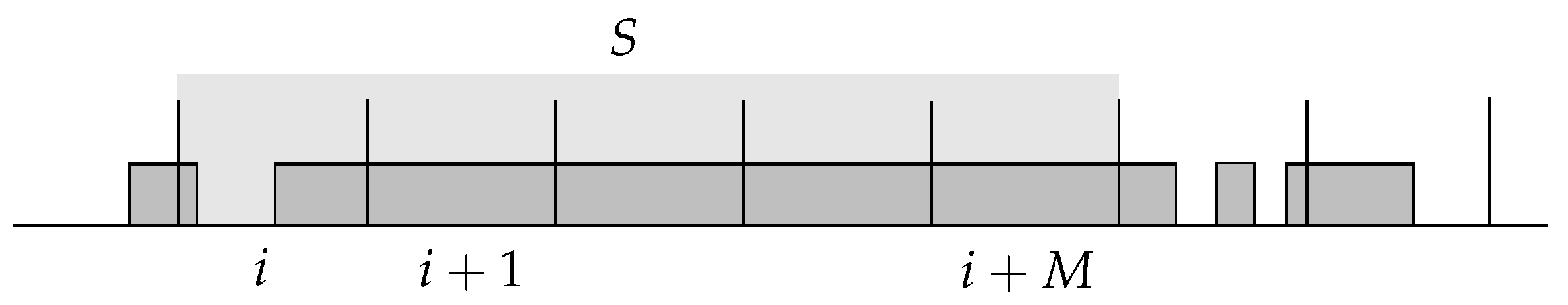
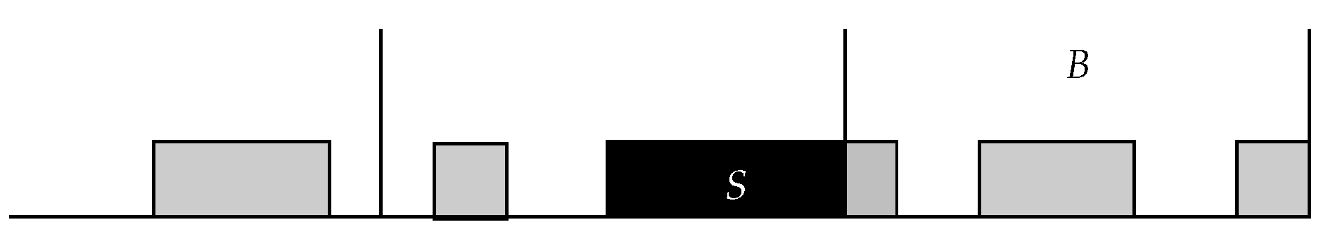
- For each block i, we define its weight to be the number of keys inserted into terminal cells found by linear probe sequences whose starting locations belong to block i. Each key, then, is inserted into the terminal cell found by the linear probe sequence that has started from the block of smaller weight.
Paper Scope
2. Background and History
2.1. Probing and Replacement
- Random Probing [16]: For every key x, the infinite sequence is assumed to be independent and uniformly distributed over . That is, we require to have an infinite sequence of truly uniform and independent hash functions. If for each key x, the first n probes of the sequence are distinct, i.e., it is a random permutation, then it is called uniform probing [1].
- Linear Probing [1]: For every key x, the first probe is assumed to be uniform on , and the next probes are defined by , for . So we only require to be a truly uniform hash function.
- Double Probing [17]: For every key x, the first probe is , and the next probes are defined by , for , where and g are truly uniform and independent hash functions.
2.2. Average Performance
2.3. Worst-Case Performance
2.4. Other Initiatives
2.5. The Multiple-Choice Paradigm
3. The Proposal
3.1. Two-Way Linear Probing
- 1.
- It chooses two initial hashing cells independently and uniformly at random, with replacement.
- 2.
- Two terminal (empty) cells are then found by linear probe sequences starting from the initial cells.
- 3.
- The key is inserted into one of these terminal cells.
- The Shorter Probe Sequence: ShortSeq Algorithm
- The Smaller Cluster: SmallCluster Algorithm
3.2. Hashing with Blocking
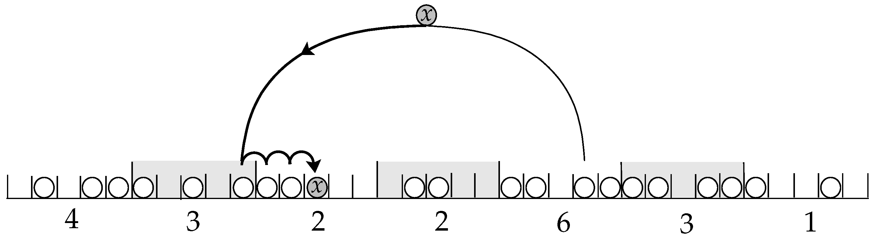
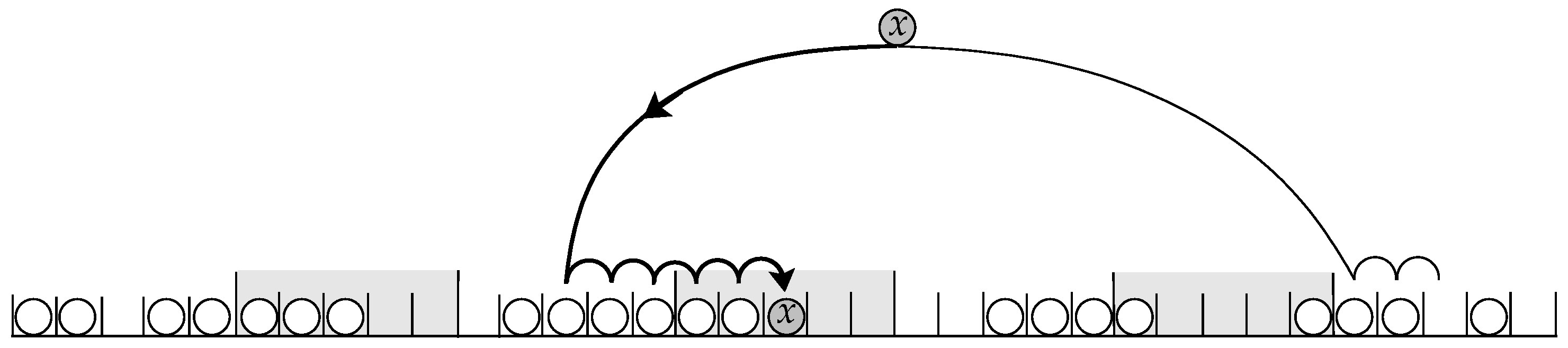
- Two-Way Locally Linear Probing: LocallyLinear Algorithm
- Two-Way Pre-Linear Probing: DecideFirst Algorithm
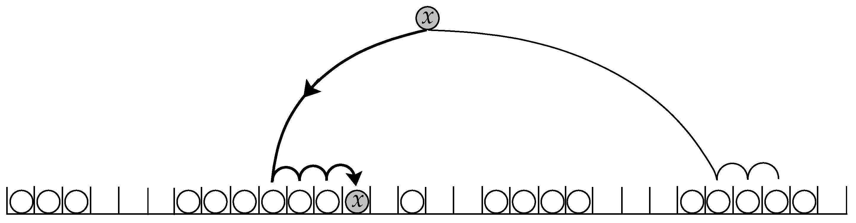
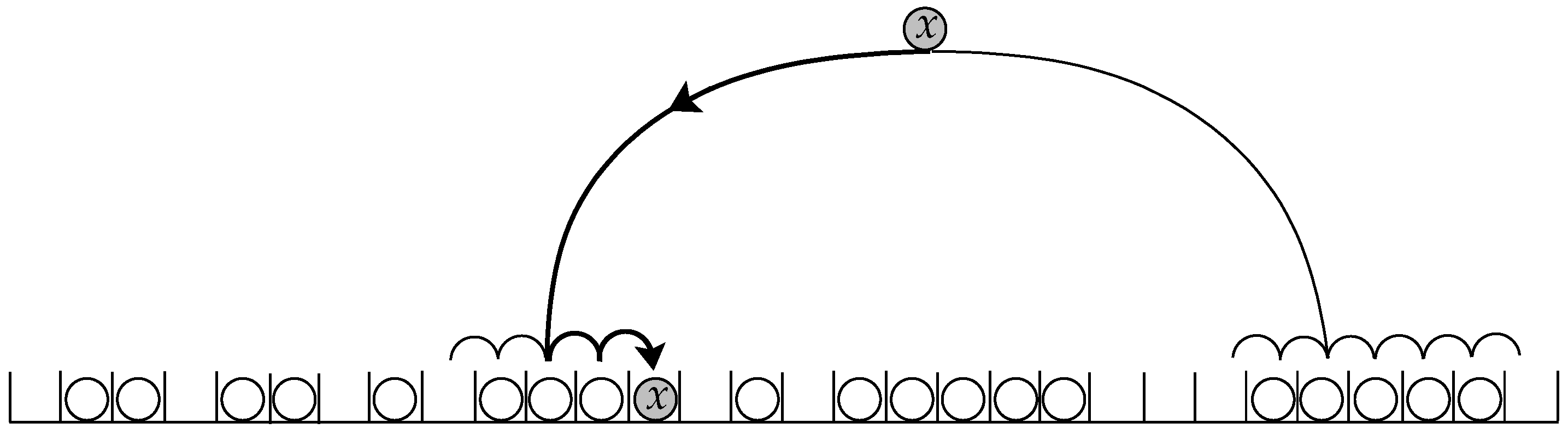
- Two-Way Post-Linear Probing: WalkFirst Algorithm
4. Lower Bounds
4.1. Universal Lower Bound
4.2. Algorithms That Behave Poorly
5. Upper Bounds
5.1. Two-Way Locally Linear Probing: LocallyLinear Algorithm
5.2. Two-Way Pre-Linear Probing: DecideFirst Algorithm
5.3. Two-Way Post-Linear Probing: WalkFirst Algorithm
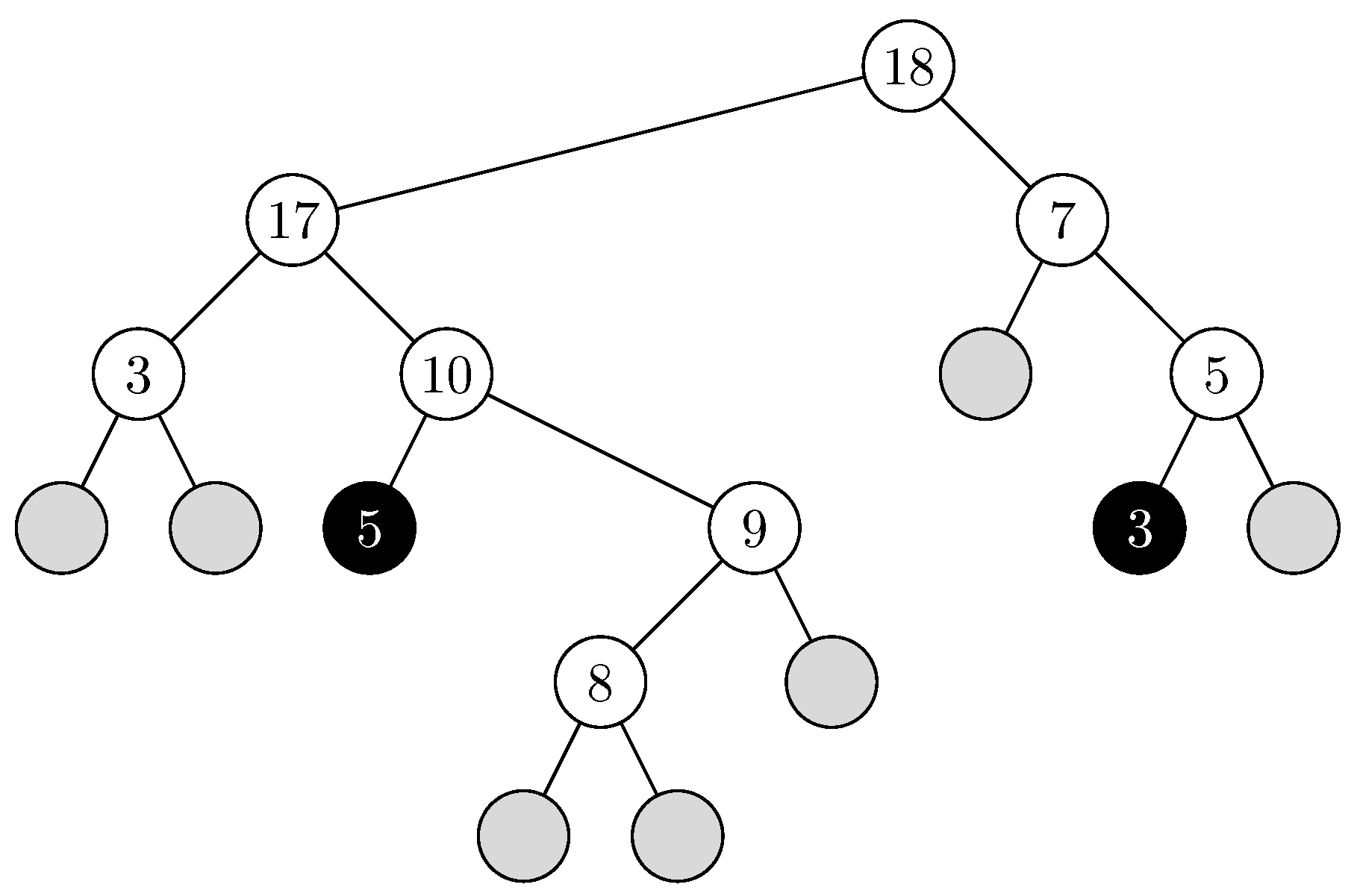
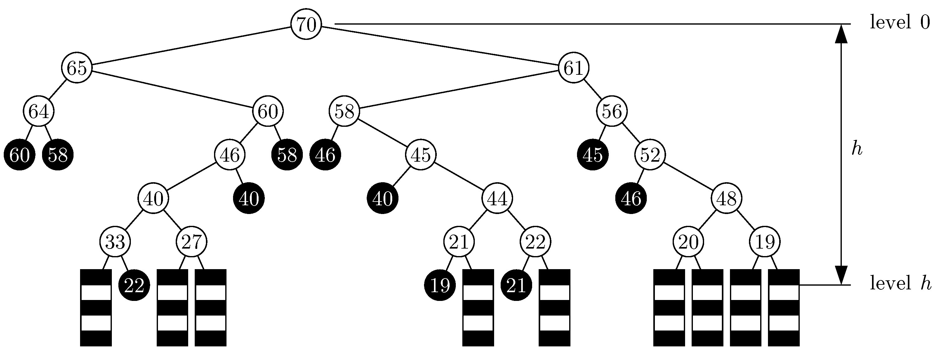
- The History Tree
- (a)
- If the block contains some keys at the time of insertion of key , and the last key inserted in that block, say , has not been encountered thus far in the bfs order of the binary tree , then the node is labeled and colored white.
- (b)
- As in case (a), except that has already been encountered in the bfs order. We distinguish such nodes by coloring them black, but they are given the same label .
- (c)
- If the block is empty at the time of insertion of key , then it is a “dead end” node without any label and it is colored gray.
- The Witness Tree
- Proof of Theorem 10.
5.4. Trade-Offs
6. Simulation Results
7. Conclusions
Author Contributions
Funding
Conflicts of Interest
Appendix A
Appendix A.1. Lemmas Needed for Theorem 10

Appendix A.2. Lemmas Needed for Theorem 7
References
- Peterson, W.W. Addressing for random-access storage. IBM J. Res. Dev. 1957, 1, 130–146. [Google Scholar] [CrossRef]
- Gonnet, G.H.; Baeza-Yates, R. Handbook of Algorithms and Data Structures; Addison-Wesley: Workingham, UK, 1991. [Google Scholar]
- Knuth, D.E. The Art of Computer Programming, Vol. 3: Sorting and Searching; Addison-Wesley: Reading, UK, 1973. [Google Scholar]
- Vitter, J.S.; Flajolet, P. Average-case analysis of algorithms and data structures. In Handbook of Theoretical Computer Science, Volume A: Algorithms and Complexity; van Leeuwen, J., Ed.; MIT Press: Amsterdam, The Netherlands, 1990; pp. 431–524. [Google Scholar]
- Janson, S.; Viola, A. A unified approach to linear probing hashing with buckets. Algorithmica 2016, 75, 724–781. [Google Scholar]
- Pagh, A.; Pagh, R.; Ružić, M. Linear probing with 5-wise independence. SIAM Rev. 2011, 53, 547–558. [Google Scholar] [CrossRef][Green Version]
- Richter, S.; Alvarez, V.; Dittrich, J. A seven-dimensional analysis of hashing methods and its implications on query processing. Porc. Vldb Endow. 2015, 9, 96–107. [Google Scholar] [CrossRef]
- Thorup, M.; Zhang, Y. Tabulation-based 5-independent hashing with applications to linear probing and second moment estimation. SIAM J. Comput. 2012, 41, 293–331. [Google Scholar] [CrossRef][Green Version]
- Pittel, B. Linear probing: The probable largest search time grows logarithmically with the number of records. J. Algorithms 1987, 8, 236–249. [Google Scholar]
- Azar, Y.; Broder, A.Z.; Karlin, A.R.; Upfal, E. Balanced allocations. SIAM J. Comput. 2000, 29, 180–200. [Google Scholar] [CrossRef]
- Vöcking, B. How asymmetry helps load balancing. J. ACM 2003, 50, 568–589. [Google Scholar] [CrossRef]
- Malalla, E. Two-Way Hashing with Separate Chaining and Linear Probing. Ph.D. Thesis, School of Computer Science, McGill University, Montreal, QC, Canada, 2004. [Google Scholar]
- Dalal, K.; Devroye, L.; Malalla, E.; McLeish, E. Two-way chaining with reassignment. SIAM J. Comput. 2005, 35, 327–340. [Google Scholar] [CrossRef]
- Berenbrink, P.; Czumaj, A.; Steger, A.; Vöcking, B. Balanced allocations: The heavily loaded case. SIAM J. Comput. 2006, 35, 1350–1385. [Google Scholar] [CrossRef]
- Malalla, E. Two-way chaining for non-uniform distributions. Int. J. Comput. Math. 2010, 87, 454–473. [Google Scholar]
- Morris, R. Scatter storage techniques. Commun. ACM 1968, 11, 38–44. [Google Scholar] [CrossRef]
- De Balbine, G. Computational Analysis of the Random Components Induced by Binary Equivalence Relations. Ph.D. Thesis, California Institute of Technology, Pasadena, CA, USA, 1969. [Google Scholar]
- Ullman, J.D. A note on the efficiency of hashing functions. J. ACM 1972, 19, 569–575. [Google Scholar]
- Yao, A.C. Uniform hashing is optimal. J. ACM 1985, 32, 687–693. [Google Scholar] [CrossRef]
- Munro, J.I.; Celis, P. Techniques for collision resolution in hash tables with open addressing. In Proceedings of the 1986 Fall Joint Computer Conference, Dallas, TX, USA, 2–6 November 1999; pp. 601–610. [Google Scholar]
- Poblete, P.V.; Munro, J.I. Last-Come-First-Served hashing. J. Algorithms 1989, 10, 228–248. [Google Scholar]
- Celis, P. Robin Hood Hashing. Ph.D. Thesis, Computer Science Department, University of Waterloo, Waterloo, ON, Canada, 1986. [Google Scholar]
- Celis, P.; Larson, P.; Munro, J.I. Robin Hood hashing (preliminary report). In Proceedings of the 26th Annual IEEE Symposium on Foundations of Computer Science (FOCS), Portland, OR, USA, 21–23 October 1985; pp. 281–288. [Google Scholar]
- Larson, P. Analysis of uniform hashing. J. ACM 1983, 30, 805–819. [Google Scholar] [CrossRef]
- Bollobás, B.; Broder, A.Z.; Simon, I. The cost distribution of clustering in random probing. J. ACM 1990, 37, 224–237. [Google Scholar]
- Knuth, D.E. Notes on “Open” Addressing. Unpublished Notes. 1963. Available online: https://jeffe.cs.illinois.edu/teaching/datastructures/2011/notes/knuth-OALP.pdf (accessed on 31 August 2023).
- Konheim, A.G.; Weiss, B. An occupancy discipline and applications. SIAM Journal on Applied Mathematics 1966, 14, 1266–1274. [Google Scholar] [CrossRef]
- Mendelson, H.; Yechiali, U. A new approach to the analysis of linear probing schemes. J. ACM 1980, 27, 474–483. [Google Scholar]
- Guibas, L.J. The analysis of hashing techniques that exhibit K-ary clustering. J. ACM 1978, 25, 544–555. [Google Scholar] [CrossRef]
- Lueker, G.S.; Molodowitch, M. More analysis of double hashing. Combinatorica 1993, 13, 83–96. [Google Scholar] [CrossRef]
- Schmidt, J.P.; Siegel, A. Double Hashing Is Computable and Randomizable with Universal Hash Functions; Submitted. A Full Version Is Available as Technical Report TR1995-686; Computer Science Department, New York University: New York, NY, USA, 1995. [Google Scholar]
- Siegel, A.; Schmidt, J.P. Closed Hashing Is Computable and Optimally Randomizable with Universal Hash Functions; Submitted. A Full Version Is Available as Technical Report TR1995-687; Computer Science Department, New York University: New York, NY, USA, 1995. [Google Scholar]
- Flajolet, P.; Poblete, P.V.; Viola, A. On the analysis of linear probing hashing. Algorithmica 1998, 22, 490–515. [Google Scholar] [CrossRef]
- Knuth, D.E. Linear probing and graphs, average-case analysis for algorithms. Algorithmica 1998, 22, 561–568. [Google Scholar] [CrossRef]
- Viola, A.; Poblete, P.V. The analysis of linear probing hashing with buckets. Algorithmica 1998, 21, 37–71. [Google Scholar] [CrossRef]
- Janson, S. Asymptotic distribution for the cost of linear probing hashing. Random Struct. Algorithms 2001, 19, 438–471. [Google Scholar] [CrossRef]
- Gonnet, G.H. Open addressing hashing with unequal-probability keys. J. Comput. Syst. Sci. 1980, 20, 354–367. [Google Scholar] [CrossRef][Green Version]
- Aldous, D. Hashing with linear probing, under non-uniform probabilities. Probab. Eng. Inform. Sci. 1988, 2, 1–14. [Google Scholar] [CrossRef]
- Pflug, G.C.; Kessler, H.W. Linear probing with a nonuniform address distribution. J. ACM 1987, 34, 397–410. [Google Scholar] [CrossRef]
- Poblete, P.V.; Viola, A.; Munro, J.I. Analyzing the LCFS linear probing hashing algorithm with the help of Maple. Maple Tech. Newlett. 1997, 4, 8–13. [Google Scholar]
- Janson, S. Individual Displacements for Linear Probing Hashing with Different Insertion Policies; Technical Report No. 35; Department of Mathematics, Uppsala University: Uppsala, Sweden, 2003. [Google Scholar]
- Viola, A. Exact distributions of individual displacements in linear probing hashing. ACM Trans. Algorithms 2005, 1, 214–242. [Google Scholar] [CrossRef]
- Chassaing, P.; Louchard, G. Phase transition for parking blocks, Brownian excursion and coalescence. Random Struct. Algorithms 2002, 21, 76–119. [Google Scholar] [CrossRef]
- Gonnet, G.H. Expected length of the longest probe sequence in hash code searching. J. ACM 1981, 28, 289–304. [Google Scholar] [CrossRef]
- Devroye, L.; Morin, P.; Viola, A. On worst-case Robin Hood hashing. SIAM J. Comput. 2004, 33, 923–936. [Google Scholar] [CrossRef]
- Gonnet, G.H.; Munro, J.I. Efficient ordering of hash tables. SIAM J. Comput. 1979, 8, 463–478. [Google Scholar] [CrossRef]
- Brent, R.P. Reducing the retrieval time of scatter storage techniques. Commun. ACM 1973, 16, 105–109. [Google Scholar] [CrossRef]
- Madison, J.A.T. Fast lookup in hash tables with direct rehashing. Comput. J. 1980, 23, 188–189. [Google Scholar] [CrossRef]
- Mallach, E.G. Scatter storage techniques: A uniform viewpoint and a method for reducing retrieval times. Comput. J. 1977, 20, 137–140. [Google Scholar] [CrossRef]
- Rivest, R.L. Optimal arrangement of keys in a hash table. J. ACM 1978, 25, 200–209. [Google Scholar] [CrossRef]
- Pagh, R.; Rodler, F.F. Cuckoo hashing. In Algorithms—ESA 2001, Proceedings of the 9th Annual European Symposium, Aarhus, Denmark, 28–31 August 2001; LNCS 2161; Springer: Berlin/Heidelberg, Germany, 2001; pp. 121–133. [Google Scholar]
- Devroye, L.; Morin, P. Cuckoo hashing: Further analysis. Inf. Process. Lett. 2003, 86, 215–219. [Google Scholar] [CrossRef]
- Östlin, A.; Pagh, R. Uniform hashing in constant time and linear space. In Proceedings of the 35th Annual ACM Symposium on Theory of Computing (STOC), San Diego, CA, USA, 9–11 June 2003; pp. 622–628. [Google Scholar]
- Dietzfelbinger, M.; Wolfel, P. Almost random graphs with simple hash functions. In Proceedings of the 35th Annual ACM Symposium on Theory of Computing (STOC), San Diego, CA, USA, 9–11 June 2003; pp. 629–638. [Google Scholar]
- Fotakis, D.; Pagh, R.; Sanders, P.; Spirakis, P. Space efficient hash tables with worst case constant access time. In STACS 2003, Proceedings of the 20th Annual Symposium on Theoretical Aspects of Computer Science, Berlin, Germany, 27 February–1 March 2003; LNCS 2607; Springer: Berlin/Heidelberg, Germany, 2003; pp. 271–282. [Google Scholar]
- Fountoulakis, N.; Panagiotou, K. Sharp Load Thresholds for Cuckoo Hashing. Random Struct. Algorithms 2012, 41, 306–333. [Google Scholar] [CrossRef]
- Lehman, E.; Panigrahy, R. 3.5-Way Cuckoo Hashing for the Price of 2-and-a-Bit. In Proceedings of the 17th Annual European Symposium, Copenhagen, Denmark, 7–9 September 2009; pp. 671–681. [Google Scholar]
- Dietzfelbinger, M.; Weidling, C. Balanced allocation and dictionaries with tightly packed constant size bins. Theor. Comput. Sci. 2007, 380, 47–68. [Google Scholar] [CrossRef]
- Fountoulakis, N.; Panagiotou, K.; Steger, A. On the Insertion Time of Cuckoo Hashing. SIAM J. Comput. 2013, 42, 2156–2181. [Google Scholar] [CrossRef]
- Frieze, A.M.; Melsted, P. Maximum Matchings in Random Bipartite Graphs and the Space Utilization of Cuckoo Hash Tables. Random Struct. Algorithms 2012, 41, 334–364. [Google Scholar] [CrossRef]
- Walzer, S. Load thresholds for cuckoo hashing with overlapping blocks. In Proceedings of the 45th International Colloquium on Automata, Languages, and Programming, Prague, Czech Republic, 9–13 July 2018; pp. 102:1–102:10. [Google Scholar]
- Frieze, A.M.; Melsted, P.; Mitzenmacher, M. An analysis of random-walk cuckoo hashing. SIAM J. Comput. 2011, 40, 291–308. [Google Scholar] [CrossRef]
- Pagh, R. Hash and displace: Efficient evaluation of minimal perfect hash functions. In Algorithms and Data Structures, Proceedings of the 6th International Workshop, WADS’99, Vancouver, BC, Canada, 11–14 August 1999; LNCS 1663; Springer: Berlin/Heidelberg, Germany, 1999; pp. 49–54. [Google Scholar]
- Pagh, R. On the cell probe complexity of membership and perfect hashing. In Proceedings of the 33rd Annual ACM Symposium on Theory of Computing (STOC), Crete, Greece, 6–8 July 2001; pp. 425–432. [Google Scholar]
- Dietzfelbinger, M.; auf der Heide, F.M. High performance universal hashing, with applications to shared memory simulations. In Data Structures and Efficient Algorithms; LNCS 594; Springer: Berlin/Heidelberg, Germany, 1992; pp. 250–269. [Google Scholar]
- Fredman, M.; Komlós, J.; Szemerédi, E. Storing a sparse table with O(1) worst case access time. J. ACM 1984, 31, 538–544. [Google Scholar] [CrossRef]
- Dietzfelbinger, M.; Karlin, A.; Mehlhorn, K.; auf der Heide, F.M.; Rohnert, H.; Tarjan, R. Dynamic perfect hashing: Upper and lower bounds. SIAM J. Comput. 1994, 23, 738–761. [Google Scholar] [CrossRef]
- Dietzfelbinger, M.; auf der Heide, F.M. A new universal class of hash functions and dynamic hashing in real time. In Automata, Languages and Programming, Proceedings of the 17th International Colloquium, Warwick University, UK, 16–20 July 1990; LNCS 443; Springer: Berlin/Heidelberg, Germany, 1990; pp. 6–19. [Google Scholar]
- Broder, A.Z.; Karlin, A. Multilevel adaptive hashing. In Proceedings of the 1st Annual ACM-SIAM Symposium on Discrete Algorithms (SODA), Salt Lake City, UT, USA, 5–8 January 2020; ACM Press: New York, NY, USA, 2000; pp. 43–53. [Google Scholar]
- Dietzfelbinger, M.; Gil, J.; Matias, Y.; Pippenger, N. Polynomial hash functions are reliable (extended abstract). In Automata, Languages and Programming, Proceedings of the 19th International Colloquium, Wien, Austria, 13–17 July 1992; LNCS 623; Springer: Berlin/Heidelberg, Germany, 1992; pp. 235–246. [Google Scholar]
- Johnson, N.L.; Kotz, S. Urn Models and Their Application: An Approach to Modern Discrete Probability Theory; John Wiley: New York, NY, USA, 1977. [Google Scholar]
- Kolchin, V.F.; Sevast’yanov, B.A.; Chistyakov, V.P. Random Allocations; V. H. Winston & Sons: Washington, DC, USA, 1978. [Google Scholar]
- Devroye, L. The expected length of the longest probe sequence for bucket searching when the distribution is not uniform. J. Algorithms 1985, 6, 1–9. [Google Scholar] [CrossRef]
- Raab, M.; Steger, A. “Balls and bins”—A simple and tight analysis. In Randomization and Approximation Techniques in Computer Science, Second International Workshop, RANDOM’98, Barcelona, Spain, 8–10 October 1998; LNCS 1518; Springer: Berlin/Heidelberg, Germany, 1998; pp. 159–170. [Google Scholar]
- Mitzenmacher, M.D. The Power of Two Choices in Randomized Load Balancing. Ph.D. Thesis, Computer Science Department, University of California at Berkeley, Berkeley, CA, USA, 1996. [Google Scholar]
- Karp, R.; Luby, M.; auf der Heide, F.M. Efficient PRAM simulation on a distributed memory machine. Algorithmica 1996, 16, 245–281. [Google Scholar] [CrossRef]
- Eager, D.L.; Lazowska, E.D.; Zahorjan, J. Adaptive load sharing in homogeneous distributed systems. IEEE Trans. Softw. Eng. 1986, 12, 662–675. [Google Scholar] [CrossRef]
- Vöcking, B. Symmetric vs. asymmetric multiple-choice algorithms. In Proceedings of the 2nd ARACNE Workshop, Aarhus, Denmark, 27 August 2001; pp. 7–15. [Google Scholar]
- Adler, M.; Berenbrink, P.; Schroeder, K. Analyzing an infinite parallel job allocation process. In Proceedings of the 6th European Symposium on Algorithms, Venice, Italy, 24–26 August 1998; pp. 417–428. [Google Scholar]
- Adler, M.; Chakrabarti, S.; Mitzenmacher, M.; Rasmussen, L. Parallel randomized load balancing. In Proceedings of the 27th Annual ACM Symposium on Theory of Computing (STOC), Las Vegas, NV, USA, 29 May–1 June 1995; pp. 238–247. [Google Scholar]
- Czumaj, A.; Stemann, V. Randomized Allocation Processes. Random Struct. Algorithms 2001, 18, 297–331. [Google Scholar] [CrossRef]
- Berenbrink, P.; Czumaj, A.; Friedetzky, T.; Vvedenskaya, N.D. Infinite parallel job allocations. In Proceedings of the 12th Annual ACM Symposium on Parallel Algorithms and Architectures (SPAA), Bar Harbor, ME, USA, 9–13 July 2000; pp. 99–108. [Google Scholar]
- Stemann, V. Parallel balanced allocations. In Proceedings of the 8th Annual ACM Symposium on Parallel Algorithms and Architectures (SPAA), Padua, Italy, 24–26 June 1996; pp. 261–269. [Google Scholar]
- Mitzenmacher, M. Studying balanced allocations with differential equations. Comb. Probab. Comput. 1999, 8, 473–482. [Google Scholar]
- Mitzenmacher, M.D.; Richa, A.; Sitaraman, R. The power of two random choices: A survey of the techniques and results. In Handbook of Randomized Computing; Pardalos, P., Rajasekaran, S., Rolim, J., Eds.; Kluwer Press: London, UK, 2000; pp. 255–305. [Google Scholar]
- Broder, A.; Mitzenmacher, M. Using multiple hash functions to improve IP lookups. In Proceedings of the 20th Annual Joint Conference of the IEEE Computer and Communications Societies (INFOCOM 2001); Full Version Available as Technical Report TR–03–00; Department of Computer Science, Harvard University: Cambridge, MA, USA, 2000; pp. 1454–1463. [Google Scholar]
- Mitzenmacher, M.; Vöcking, B. The asymptotics of Selecting the shortest of two, improved. In Proceedings of the 37th Annual Allerton Conference on Communication, Control, and Computing, Monticello, IL, USA, 22–23 September 1998; pp. 326–327. [Google Scholar]
- Wu, J.; Kobbelt, L. Fast mesh decimation by multiple-choice techniques. In Proceedings of the Vision, Modeling, and Visualization, Erlangen, Germany, 20–22 November 2002; pp. 241–248. [Google Scholar]
- Siegel, A. On universal classes of extremely random constant time hash functions and their time-space tradeoff. Technical Report TR1995-684, Computer Science Department, New York University, 1995. A previous version appeared under the title “On universal classes of fast high performance hash functions, their time-space tradeoff and their applications”. In Proceedings of the 30th Annual IEEE Symposium on Foundations of Computer Science (FOCS), Triangle Park, NC, USA, 30 October–1 November 1989; pp. 20–25. [Google Scholar]
- Auf der Heide, F.M.; Scheideler, C.; Stemann, V. Exploiting storage redundancy to speed up randomized shared memory simulations. Theor. Comput. Sci. 1996, 162, 245–281. [Google Scholar]
- Schickinger, T.; Steger, A. Simplified witness tree arguments. In SOFSEM 2000: Theory and Practice of Informatics, Proceedings of the 27th Annual Conference on Current Trends in Theory and Practice of Informatics, Milovy, Czech Republic, 25 November–2 December 2000; LNCS 1963; Springer: Berlin/Heidelberg, Germany, 2000; pp. 71–78. [Google Scholar]
- Cole, R.; Maggs, B.M.; auf der Heide, F.M.; Mitzenmacher, M.; Richa, A.W.; Schroeder, K.; Sitaraman, R.K.; Voecking, B. Randomized protocols for low-congestion circuit routing in multistage interconnection networks. In Proceedings of the 29th Annual ACM Symposium on the Theory of Computing (STOC), El Paso, TX, USA, 4–6 May 1998; pp. 378–388. [Google Scholar]
- Cole, R.; Frieze, A.; Maggs, B.M.; Mitzenmacher, M.; Richa, A.W.; Sitaraman, R.K.; Upfal, E. On balls and bins with deletions. In Randomization and Approximation Techniques in Computer Science, Proceedings of the 2nd International Workshop, RANDOM’98, Barcelona, Spain, 8–10 October 1998; LNCS 1518; Springer: Berlin/Heidelberg, Germany, 1998; pp. 145–158. [Google Scholar]
- Swain, S.N.; Subudhi, A. A novel RACH scheme for efficient access in 5G and Beyond betworks using hash function. In Proceedings of the 2022 IEEE Future Networks World Forum (FNWF), Montreal, QC, Canada, 10–14 October 2022; pp. 75–82. [Google Scholar]
- Guo, J.; Liu, Z.; Tian, S.; Huang, F.; Li, J.; Li, X.; Igorevich, K.K.; Ma, J. TFL-DT: A trust evaluation scheme for federated learning in digital twin for mobile networks. IEEE J. Sel. Areas Commun. 2023, 41, 3548–3560. [Google Scholar] [CrossRef]
- Okamoto, M. Some inequalities relating to the partial sum of binomial probabilities. Ann. Math. Stat. 1958, 10, 29–35. [Google Scholar] [CrossRef]
- Dubhashi, D.; Ranjan, D. Balls and bins: A study in negative dependence. Random Struct. Algorithms 1998, 13, 99–124. [Google Scholar] [CrossRef]
- Esary, J.D.; Proschan, F.; Walkup, D.W. Association of random variables, with applications. Ann. Math. Stat. 1967, 38, 1466–1474. [Google Scholar] [CrossRef]
- Joag-Dev, K.; Proschan, F. Negative association of random variables, with applications. Ann. Stat. 1983, 11, 286–295. [Google Scholar] [CrossRef]


| n |
ClassicLinear Insert/Search Time |
ShortSeq Insert/Search Time |
SmallCluster Search Time |
SmallCluster InsertTime | |||||
|---|---|---|---|---|---|---|---|---|---|
| Avg | Max | Avg | Max | Avg | Max | Avg | Max | ||
| 0.4 | 1.33 | 5.75 | 1.28 | 4.57 | 1.28 | 4.69 | 1.50 | 9.96 | |
| 0.9 | 4.38 | 68.15 | 2.86 | 39.72 | 3.05 | 35.69 | 6.63 | 71.84 | |
| 0.4 | 1.33 | 10.66 | 1.28 | 7.35 | 1.29 | 7.49 | 1.52 | 14.29 | |
| 0.9 | 5.39 | 275.91 | 2.90 | 78.21 | 3.07 | 66.03 | 6.91 | 118.34 | |
| 0.4 | 1.33 | 16.90 | 1.28 | 10.30 | 1.29 | 10.14 | 1.52 | 18.05 | |
| 0.9 | 5.49 | 581.70 | 2.89 | 120.32 | 3.07 | 94.58 | 6.92 | 155.36 | |
| 0.4 | 1.33 | 23.64 | 1.28 | 13.24 | 1.29 | 13.03 | 1.52 | 21.41 | |
| 0.9 | 5.50 | 956.02 | 2.89 | 164.54 | 3.07 | 122.65 | 6.92 | 189.22 | |
| 0.4 | 1.33 | 26.94 | 1.28 | 14.94 | 1.29 | 14.44 | 1.52 | 23.33 | |
| 0.9 | 5.50 | 1157.34 | 2.89 | 188.02 | 3.07 | 136.62 | 6.93 | 205.91 | |
| n | ClassicLinear | ShortSeq | SmallCluster | ||||
|---|---|---|---|---|---|---|---|
| Avg | Max | Avg | Max | Avg | Max | ||
| 0.4 | 2.02 | 8.32 | 1.76 | 6.05 | 1.76 | 5.90 | |
| 0.9 | 15.10 | 87.63 | 12.27 | 50.19 | 12.26 | 43.84 | |
| 0.4 | 2.03 | 14.95 | 1.75 | 9.48 | 1.75 | 9.05 | |
| 0.9 | 15.17 | 337.22 | 12.35 | 106.24 | 12.34 | 78.75 | |
| 0.4 | 2.02 | 22.54 | 1.75 | 12.76 | 1.75 | 12.08 | |
| 0.9 | 15.16 | 678.12 | 12.36 | 155.26 | 12.36 | 107.18 | |
| 0.4 | 2.02 | 29.92 | 1.75 | 16.05 | 1.75 | 15.22 | |
| 0.9 | 15.17 | 1091.03 | 12.35 | 203.16 | 12.35 | 136.19 | |
| 0.4 | 2.02 | 33.81 | 1.75 | 17.74 | 1.75 | 16.65 | |
| 0.9 | 15.17 | 1309.04 | 12.35 | 226.44 | 12.35 | 150.23 | |
| n | LocallyLinear | WalkFirst | DecideFirst | ||||
|---|---|---|---|---|---|---|---|
| Avg | Max | Avg | Max | Avg | Max | ||
| 0.4 | 1.73 | 4.73 | 1.78 | 5.32 | 1.75 | 5.26 | |
| 0.9 | 4.76 | 36.23 | 4.76 | 43.98 | 5.06 | 59.69 | |
| 0.4 | 1.74 | 6.25 | 1.80 | 7.86 | 1.78 | 7.88 | |
| 0.9 | 4.76 | 47.66 | 4.80 | 67.04 | 4.94 | 108.97 | |
| 0.4 | 1.76 | 7.93 | 1.80 | 9.84 | 1.78 | 10.08 | |
| 0.9 | 4.78 | 56.40 | 4.89 | 89.77 | 5.18 | 137.51 | |
| 0.4 | 1.76 | 8.42 | 1.81 | 12.08 | 1.79 | 12.39 | |
| 0.9 | 4.77 | 65.07 | 4.98 | 108.24 | 5.26 | 162.04 | |
| 0.4 | 1.76 | 9.18 | 1.81 | 12.88 | 1.79 | 13.37 | |
| 0.9 | 4.80 | 71.69 | 5.04 | 118.06 | 5.32 | 181.46 | |
| n | LocallyLinear | WalkFirst | DecideFirst | ||||
|---|---|---|---|---|---|---|---|
| Avg | Max | Avg | Max | Avg | Max | ||
| 0.4 | 1.14 | 2.78 | 2.52 | 6.05 | 1.15 | 3.30 | |
| 0.9 | 2.89 | 22.60 | 6.19 | 48.00 | 3.19 | 42.64 | |
| 0.4 | 1.14 | 3.38 | 2.53 | 8.48 | 1.17 | 5.19 | |
| 0.9 | 2.91 | 27.22 | 6.28 | 69.30 | 3.16 | 84.52 | |
| 0.4 | 1.15 | 4.08 | 2.53 | 10.40 | 1.17 | 6.56 | |
| 0.9 | 2.84 | 31.21 | 6.43 | 91.21 | 3.17 | 106.09 | |
| 0.4 | 1.15 | 4.64 | 2.54 | 12.58 | 1.18 | 8.16 | |
| 0.9 | 2.89 | 35.21 | 6.54 | 109.71 | 3.22 | 117.42 | |
| 0.4 | 1.15 | 4.99 | 2.54 | 13.41 | 1.18 | 8.83 | |
| 0.9 | 2.91 | 38.75 | 6.61 | 119.07 | 3.26 | 132.83 | |
| n | LocallyLinear | WalkFirst | DecideFirst | ||||
|---|---|---|---|---|---|---|---|
| Avg | Max | Avg | Max | Avg | Max | ||
| 0.4 | 1.57 | 4.34 | 1.65 | 4.70 | 1.63 | 4.81 | |
| 0.9 | 12.18 | 33.35 | 12.54 | 34.40 | 13.48 | 47.76 | |
| 0.4 | 1.62 | 6.06 | 1.68 | 6.32 | 1.68 | 6.82 | |
| 0.9 | 12.42 | 48.76 | 12.78 | 51.80 | 13.45 | 94.98 | |
| 0.4 | 1.62 | 7.14 | 1.68 | 7.31 | 1.68 | 8.92 | |
| 0.9 | 12.66 | 59.61 | 12.98 | 62.24 | 13.53 | 125.40 | |
| 0.4 | 1.65 | 8.25 | 1.71 | 8.50 | 1.71 | 10.76 | |
| 0.9 | 12.83 | 67.23 | 13.11 | 69.45 | 13.62 | 145.30 | |
| 0.4 | 1.62 | 8.90 | 1.71 | 8.95 | 1.71 | 11.46 | |
| 0.9 | 12.72 | 65.58 | 13.19 | 73.22 | 13.66 | 164.45 | |
Disclaimer/Publisher’s Note: The statements, opinions and data contained in all publications are solely those of the individual author(s) and contributor(s) and not of MDPI and/or the editor(s). MDPI and/or the editor(s) disclaim responsibility for any injury to people or property resulting from any ideas, methods, instructions or products referred to in the content. |
© 2023 by the authors. Licensee MDPI, Basel, Switzerland. This article is an open access article distributed under the terms and conditions of the Creative Commons Attribution (CC BY) license (https://creativecommons.org/licenses/by/4.0/).
Share and Cite
Dalal, K.; Devroye, L.; Malalla, E. Two-Way Linear Probing Revisited. Algorithms 2023, 16, 500. https://doi.org/10.3390/a16110500
Dalal K, Devroye L, Malalla E. Two-Way Linear Probing Revisited. Algorithms. 2023; 16(11):500. https://doi.org/10.3390/a16110500
Chicago/Turabian StyleDalal, Ketan, Luc Devroye, and Ebrahim Malalla. 2023. "Two-Way Linear Probing Revisited" Algorithms 16, no. 11: 500. https://doi.org/10.3390/a16110500
APA StyleDalal, K., Devroye, L., & Malalla, E. (2023). Two-Way Linear Probing Revisited. Algorithms, 16(11), 500. https://doi.org/10.3390/a16110500