Abstract
Brain–computer interfaces (BCIs) based on steady-state visually evoked potentials (SSVEPs) are inexpensive and do not require user training. However, the highly personalized reaction to visual stimulation is an obstacle to the wider application of this technique, as it can be ineffective, tiring, or even harmful at certain frequencies. In our experimental study, we proposed a new approach to the selection of optimal frequencies of photostimulation. By using a custom photostimulation device, we covered a frequency range from 5 to 25 Hz with 1 Hz increments, recording the subjects’ brainwave activity (EEG) and analyzing the signal-to-noise ratio (SNR) changes at the corresponding frequencies. The proposed set of SNR-based coefficients and the discomfort index, determined by the ratio of theta and beta rhythms in the EEG signal, enables the automation of obtaining the recommended stimulation frequencies for use in SSVEP-based BCIs.
1. Introduction
As graphical user interface (GUI) technology is nearing its 50th anniversary, humans are actively seeking new modes of interaction with machines. A user, considered as a source of information, can use their gestures, voice, eye movements, etc., to generate control commands or actions. A promising communication channel is the one based on the neural activity of the brain (hence, the so-called brain–computer interface (BCI)). Its important advantage is accessibility, even for people whose motor reactions are disrupted or cease completely. For healthy people, BCIs hold a compelling promise to “read one’s mind”, especially when in conjunction with booming artificial intelligence (AI) technologies [1]. Although BCI technology is not yet fully mature, it has been applied to control a wide variety of devices, including computers, motorized wheelchairs [2], and exoskeletons. It is used to monitor cognitive states, mental loads, and fatigue [3], as well as in rehabilitation systems for stroke patients [4].
There are many paradigms and approaches on the basis of which BCIs are built and function [5]. The one that demonstrates the highest interaction accuracy and speed [6] is steady-state visually evoked potential (SSVEP), which involves a specific neuronal response that occurs as a result of presenting a periodic visual stimulus to a subject [7]. This reaction is mainly localized to the occipital region of the cerebral cortex and can be recorded in the O1, O2, and Oz leads placed according to the “10–20” system for electroencephalography (EEG) [8]. The main characteristics of these potentials are their frequencies, which strictly depend on the frequencies of visual stimuli, and power, which is usually significantly higher than the power of the baseline brainwave activity. The widely claimed advantages of SSVEP-based BCIs include the following [9]:
- The high speed of the information transfer;
- The minimal time required for user training and relative ease of installation;
- The safety for the users.
The aforementioned immaturity of the BCI technology leaves much to be desired for each of the above points. First, much of the current research in the field is focused on the light stimuli of high frequencies (for EEG signals, this means more than 30 Hz [10]) to enhance the information transfer rate (ITR) or effective bit rate, as introduced in [11], and reported on in BCI studies. ITR is a common metric in SSVEP-BCI interfaces, aiding in the estimation and comparison of different identification algorithms by combining speed and accuracy. Indeed, the low-frequency range of EEG signals is affected by high-amplitude artifacts, such as EOG artifacts (concentrated in the frequency range of 1 to 5 Hz [12]). Moreover, it is overlapped by a more powerful alpha-rhythm of the EEG signal, concentrated in the frequency range of 8 to 14 Hz. However, SSVEP potentials are usually most intense in the frequency range of around 15 Hz, and the power of the evoked potential decreases with the increase of the light stimulus frequency [13].
Second, BCIs are rather less universal than most other human–machine interface modes, as the former generally require calibration and adaptation to the user’s individual characteristics. SSVEP-based BCIs have a wide scope of applications, ranging from controlling smart home devices [14] to enabling communication with patients with disorders of consciousness and facilitating the rehabilitation of individuals after severe head and spinal cord injuries [15,16]. In these scenarios, the usability and minimal training duration required to ensure reliable operation take precedence. Indeed, as mentioned above, in some people, the response level to a certain stimulus frequency may be too low relative to the EEG signal itself, making this frequency unsuitable for use [10]. This makes it difficult to build a universal BCI that uses a single frequency range for its users. The need for calibration is recognized as a major obstacle for the wider BCI development and hurts the overall user experience (UX) [17,18]. The currently popular approach to the so-called subject calibration problem is “subject-transfer” [19], which largely corresponds to the general transfer learning approaches in AI-ML: instance-based, parameter-based, or feature-based [20]. Correspondingly, methods and models that improve the trade-off between the calibration effort and the BCI performance move the field forward, but this issue is far from being resolved yet.
Third, the claimed safety of BCIs is rather situational. Even if we do not consider brain-invasive techniques, the photo stimuli can cause strong fatigue (particularly to the eyes) and even provoke an epileptic seizure for individuals suffering from photosensitive epilepsy [21]. Research suggests that these risks are frequency-specific, being more prone to the middle-frequency range of EEG signals (from 12 to 30 Hz) [10], and user group-specific [22]. Zhang and colleagues demonstrated in their recent study that SSVEP target–classification accuracy decreases under the influence of stress [23]. To assess the extent of the impact of periodic photostimulation on the subjective emotional state of participants and to objectify the degree of discomfort experienced during interaction with neurointerfaces, researchers in this field employ indices that are specifically derived from the power ratios of major EEG frequency bands. For instance, theta–beta ratio [24], theta–alpha ratio [25], and frontal alpha asymmetry [26] have frequently been used as such indices in scientific literature. Incorporating these index values into the development of an algorithm for individually tailored stimulation frequencies could represent a crucial step toward creating more personalized and user-friendly interfaces.
As any interfacing technology matures, considerations of usefulness are supplemented by those of usability. BCI is no exception in this regard. About 10 years ago, an editorial in a dedicated Special Issue of Ergonomics noted that “for people with motor disabilities, the ease and convenience of use … may be as important as speed of communication” [27]. Indeed, calls for considering UX in BCI began over a decade ago [28,29]. Currently, there is a growing interest in BCI usability evaluations, encompassing both objective and subjective measures. Clearly, this implies the need to extend the three points discussed above. A transition from a user interface (UI) to UX requires, at the very least, adding user satisfaction to the puzzle.
The main research question of our study can be formulated as follows: Is it possible to determine, based on the recorded EEG signal, whether a given photostimuli frequency is optimal in a given range for a particular person? Regarding the selection of the optimal stimulation frequency for the stable reproduction of the maximum SSVEP amplitude, opinions among researchers in the scientific community vary significantly. Broad ranges for observing SSVEP cover frequencies of 8.5–15 Hz [30], 12–18 Hz [31], or 12–30 Hz [32]. The wide variety of results obtained reflect the individual characteristics of the brain’s background state, influencing subsequent functional activity, not only of the visual system but also the outcomes of the default mode network’s interaction with other neural systems [33], making the aforementioned aim of our current study relevant. Solving this problem and improving the selection of individual photostimulus frequencies can make BCI usage more effective and satisfying for the users, by (1) increasing the information transfer rate (ITR), which in the case of BCIs is highly dependent on the calibration process, and (2) significantly improving the user experience by using stimulation frequencies that do not cause excessive fatigue or stress in the users. This is especially relevant for people who experience visual fatigue when using this type of BCI. All of these factors could enhance the acceptance of BCIs outside of research settings and foster their integration into daily life.
The remainder of our paper is structured as follows. In Section 2, we provide an overview of related work on BCI calibration, emphasizing the integration of usability and UX concepts. We also advocate for the EEG theta-to-beta measurement as indicative of user satisfaction. In Section 3, we present the algorithm for selecting BCI frequencies; in Section 4, we describe the essential coefficients. Section 5 is dedicated to the experimental evaluation of the proposed algorithm. In the final section, we summarize and discuss our contributions.
2. Related Work
2.1. BCI Applications
Nowadays, brain–computer interfaces are being applied in many fields and for many purposes. Many different paradigms are being used to design them (the SSVEP paradigm we have chosen is just one of them). It is difficult to fully cover these areas, and presented here is just a fraction of the research aimed at enhancing quality of life.
An important direction in this field involves the use of BCIs to restore the function of the cerebral cortex when it is damaged. This is achieved through the introduction of biological feedback. Reference [34] showed—for the first time—that with the help of invasive BCIs, it is possible to restore movement to paralyzed limbs in people suffering from “locked-in syndrome” (LIS). This condition is characterized by a complete loss of speech and paralysis while maintaining consciousness and sensitivity.
BCIs are also used for cursor control, text input, and forming commands for robots. An interesting example is presented in reference [35], where people with spinal cord injuries were able to modulate neural activity associated with the intention to move, even 3 years after the injury.
In recent studies, BCIs were created that could automatically recognize speech from neural activities recorded using EEGs, as well as reconstruct whole sentences from thoughts with a limited vocabulary [36]. Another line of research demonstrates the possibility of controlling a patient’s prosthetics or exoskeletons based on neural activity recorded using EEGs [37]. This opens up new perspectives for reproducing fine motor skills with prosthetics in the future.
A recent study introduced an unsupervised data-driven pipeline for rejecting blink and muscle artifacts in EEG time series for use in motor imagery (MI)-based BCIs integrated with the Internet of Medical Things (IoMT) [38]. Using this approach reduces processing times, resource demands, and reliance on human intervention, making it a promising avenue for crafting efficient, user-friendly real-time BCI systems. Moreover, the technique proposed by the authors to enhance TL-CNN classification between Mex and MI finger-pinching actions is superior to other state-of-the-art methods, which makes it promising for further development and implementation in practice.
2.2. SSVEP-Based BCI Enhancements
As a rule, scalp electroencephalography (EEG) is used as a tool to provide continuous registration of a user’s neural activity for further transmission to BCIs. The EEG signals have high temporal resolution [9,39], and the approach involves a non-invasive process of measuring the electrical activity of the cerebral cortex and does not require surgical intervention. This provides a high safety level for users of such BCIs, compared to BCIs based on electrocorticography (ECoG) [40]. The latter requires mandatory surgical intervention and, thus, poses a high level of risk, making EEG-based BCIs a safer and more promising technology for universal application.
It is recognized that BCI performance, which has been foremost associated with information transfer rates, is considerably better with calibration than in calibration-free schemes [41]. With respect to SSVEP-based BCIs, it is believed that a subject-specific type of calibration is capable of yielding the best performance. However, the time and effort spent on such individual training sessions are considered to be the most serious disadvantages of this approach [42]. Correspondingly, up-to-date research in the field focuses on (a) reducing the data amounts that need to be gathered from a particular subject by reusing some existing data [41], (b) collecting the data more intensively, e.g., through several channels [43], and (c) making more intensive use of available data via smarter calibration algorithms [33].
2.3. BCI Usability and User Satisfaction
While the safety of modern BCIs is well-established and performance remains a primary research focus, calibration algorithms that consider interface usability are relative new. BCI-related studies that follow a user-centered approach define usability in terms of effectiveness (accuracy), efficiency (ITR and subjective workloads), and user satisfaction [44].
Selection algorithms that consider the user’s emotional state and subjective comfort during BCI interactions can help lead to new levels of user experience. However, there is a certain disparity in how exactly the registered EEG signals should be used to automatically infer various dimensions of user satisfaction. Y.N. Ortega and co-authors have exhaustively addressed this in their works, recently culminating in a connection between potential EEG signal characteristics and usability measures, as presented in [45].
As mentioned in [46], using flicker frequencies in the range of 4–30 Hz can lead to visual fatigue. Thus, it is important to find frequencies at which the interaction will be the most effective and the person experiences minimal discomfort in using BCIs [47]. Various methods are employed to minimize the discomfort; for example, [46] proposed using a chessboard stimulus, which allows for reducing user discomfort without compromising performance. In turn, we suggest taking user satisfaction into account when selecting an individual frequency for BCI.
The safety of using brain–computer interfaces is a determining factor that allows them to be integrated into various aspects of our lives; therefore, this factor should be approached with the utmost seriousness and attention. In experiments based on SSVEP, the presentation of rhythmic visual stimuli potentially has the ability to induce epileptic activity and trigger seizures. However, in our study, participants over 18 years old without a history of epileptic seizures in their medical records were involved, and the likelihood that the current experimental protocol could elicit such pathological brain activity was extremely low. Additionally, after undergoing experimental stimulation without any negative effects, the probability of experiencing seizures during subsequent long-term use of BCIs becomes nearly zero. This is why we deemed it unnecessary to account for this factor or develop a special index that could consider its influence.
3. Selection Criteria of BCI Frequencies
In our study, we propose an algorithm for selecting recommended photostimulation frequencies for SSVEP-based BCIs. The goal of the algorithm is to choose the individual photostimulation frequencies that would be the most suitable for each user. We suggest that the following individual user response characteristics be considered in this algorithm:
- Reaction onset speed as a response to the presented visual stimuli;
- Ability to maintain a stable response at an acceptable level during a continuous visual stimuli presentation;
- User satisfaction with the presented photostimulus.
The reaction onset speed is an extremely important factor since it directly affects how quickly the user can send commands to the BCI. We hypothesize that by excluding photostimuli to which the user does not respond within a reasonable timeframe, and focusing solely on frequencies with the quickest reaction speeds, BCI performance will see significant improvement [13]. In this paper, we consider a stimuli frequency range from 5 to 25 Hz, and use a threshold method based on the signal-to-noise ratio (SNR) to measure the reaction speed.
The stability of the user response level is another important criterion. The more stable the response level, the higher the probability of the correct recognition of the SSVEP potential by the neurointerface. Each user has an individual response to each presented frequency, which will be further demonstrated in this study.
Finally, the user’s satisfaction, when presented with a given photostimulus frequency, is another equally important factor. The photostimuli should not cause discomfort or fatigue to the user when using the neurointerface, as this can negatively affect the duration of comfortable interaction with it.
Many scientific publications usually do not consider the possibility of response occurrences at multiples of stimulation frequencies (higher harmonics) when detecting SSVEP responses. In the proposed algorithm, we analyze the fundamental frequency of photostimulus f, as well as the second harmonic stimulation frequency 2*f when estimating the reaction onset and SSVEP response stability. This allows us to take into account individual user characteristics and expand the frequency range, especially in the low-frequency range (8–15 Hz), where SNR may be low.
Although SSVEP-based BCIs are quite attractive for solving a variety of practical tasks, as mentioned earlier, it should be noted that the user’s reaction may be unpredictable. The response to individual frequencies of visual stimulation by a particular person may be so uncertain that the algorithm will not be able to detect the response. This should certainly be taken into account, and only frequencies with the highest probability of detection should be used.
Other important UX components are the speed and quality of communication. The information transfer rate (ITR) is used for this purpose, which is measured in bits/min [48]. This parameter can be calculated using the following formula:
where P is the prediction accuracy (in the range of 0 to 1), M is the stimuli number, and T is the stimulation duration in seconds. In most studies, accuracy is calculated as the ratio of correct predictions in the experiment to the total number of predictions in the experiment.
Thus, communication speed can be increased by increasing accuracy, which depends on the used method. Another option is to reduce the stimulation time. However, it should be noted that reducing the stimulation time will lead to a decrease in BCI accuracy. Therefore, one way to increase ITR is to select the optimal stimulation duration. Moreover, stimuli frequencies also influence the results; thus, another way to increase the ITR in SSVEP-based BCIs is to choose frequencies for stimulation that elicit the fastest and/or most pronounced responses.
User satisfaction, as mentioned earlier, is also an important component of UX. In the current study, we employ the theta-to-beta ratio. This approach has been used with reasonable success in previous work, reflecting the stress in VR/AR users [49]. We used the theta-to-beta ratio as the discomfort index. Indeed, existing literature closely associates the theta-to-beta ratio with manifestations of stress and anxiety [50,51], motivation [52], and the influence of emotional factors on cognitive processes, such as attention [24]. All of these are essential components for successful human interactions with BCIs. To our knowledge, this is the first explicit attempt that takes into account emotional and motivational factors while training or calibrating BCIs. The theta-to-beta ratio was calculated based on the averaged powers of EEG theta (4–8 Hz) and beta (13–29 Hz) bands, derived from the two frontal leads, namely, F3 and F4.
4. BCI Frequency Selection Coefficients
To quantitatively assess the characteristics of the user’s reaction to the photostimulus that we have described and to obtain a list of recommended frequencies, we introduce a set of coefficients:
- Reaction speed coefficient ;
- Threshold overcoming coefficient ;
- Frequency applicability coefficient ;
- Discomfort coefficient .
As mentioned above, when presenting a photostimulus with the frequency , we analyze the user’s reaction, not only at the fundamental frequency but also at the second harmonic frequency. We will denote these frequencies as and for the fundamental and second harmonic frequencies, respectively. Thus, coefficients 1 to 3 will be calculated in two instances for each photostimulus. The first three coefficients are calculated for occipital EEG leads O1, O2, and Oz, since these are the leads in which the SSVEP potential appears in response to the presented photostimulus. To obtain these coefficients, it is necessary to calculate the SNR and the threshold values for both and frequencies. The SNR of the EEG signal at frequency is calculated by the following expression [31]:
where is the signal magnitude at frequency , obtained as a result of the calculation of a single-sided FFT, = 4 is the total number of harmonics around in the signal spectrum considered as noise, and is the frequency resolution.
During the presentation of each 60 s photostimulus, we record a fragment of the EEG signal and then divide it into a set of windows of 3 s durations and 50% overlap between the windows. For each obtained window, we compute the SNR at frequencies of and using Equation (1), thus obtaining two vectors to demonstrate how the SNR for frequencies and changed during the photostimulation. To compute the threshold value, we take a fragment of the EEG signal, where no photostimuli or any other stimuli or artifacts are presented. As in the previous example, this fragment is divided into 3 s windows set with 50% overlap between the windows. For each obtained window, the SNR vectors for frequencies and are calculated using Equation (1). Then, to obtain the threshold values for and frequencies, we use the following expression:
where is the mean value of SNR for the obtained windows at frequency , is the standard deviation of SNR at frequency , and the coefficient is equal to 3. Thus, if we consider the value of the SNR at a given frequency outside the stimulation period as a random variable, and then apply the three-sigma rule to it, we will obtain a threshold value. Exceeding this threshold with a probability of 99.7% would not occur under normal conditions (without the presentation of photo stimuli). After computing these parameters, the coefficients we proposed can be computed.
The response speed coefficient represents how fast the SSVEP potential’s value at frequency reaches the threshold value, where it can be recognized in the BCI. This coefficient is computed by Equation (3) for frequencies and , and takes values from 0 to 1, where values close to 1 mean the fastest responses and values close to 0 mean the slowest responses. Coefficient values equal to 0 indicate a complete absence of reaction.
where is the time in seconds from the start of the photostimulus presentation to the first overshoot of , and t is the total duration of the stimulation, which, in our case, is equal to 60 s.
The threshold overcoming coefficient represents how stable during the presentation of the photostimulus the SSVEP potential exceeds the threshold value at the given frequency. This coefficient is computed by Equation (4) for frequencies and , and takes values from 0 to 1, where values close to 1 mean the most stable responses and values close to 0 mean the most unstable responses. Coefficient values equal to 0 indicate a complete absence of reaction.
where is the number of windows at which at frequency exceeds the threshold value , and is the total number of windows during stimulation. The windows were selected in the same manner as for Equation (1).
The frequency applicability coefficient is introduced to combine the coefficients and into a single coefficient. The coefficient shows how generally suitable the selected frequency is for the fast and stable recognition of the photostimulus frequency in BCIs. This coefficient is calculated for frequencies and by Equation (5) and takes values from 0 to 1. Coefficient values close to 1 mean the most optimal in terms of speed and stability of frequency response, and values close to 0 mean the most suboptimal.
where denotes the response speed coefficient at frequency , and is the threshold overcoming coefficient for frequency .
The average frequency applicability coefficient is calculated by taking the average of the two coefficients obtained for the photostimulation at frequency using Equation (6). This coefficient takes values from 0 to 1 and represents how capable the photostimulus is to evoke a high-quality SSVEP response at both the fundamental and second harmonic frequencies simultaneously. Values close to 1 mean the stimulation frequencies with the highest quality SSVEP response in terms of the speed and stability of the frequency response at the first two harmonics.
where represents the applicability coefficient of frequency at the fundamental harmonic, and represents the applicability coefficient of frequency at the second harmonic.
The discomfort index was defined as a ratio of absolute theta power (4–8 Hz) divided by absolute beta power (13–30 Hz) averaged over F3 and F4 frontal electrodes, capturing the neural signals coming from the left and right hemispheres, respectively (Equation (7)). To extract EEG powers in the above-mentioned frequency bands, fast Fourier transform (FFT) was applied (Hanning window length 10) in the MNE Python.
where denotes the discomfort index for the frequency of photostimulation , and are the signal magnitudes at frequency from electrodes F3 and F4, respectively, during light stimulations at frequency .
The discomfort coefficient is introduced in order to normalize the discomfort index in the range of 0 to 1 and is intended to standardize this indicator for different subjects when using our developed application for selecting recommended frequencies. This coefficient is calculated using the min–max normalization formula and takes values from 0 to 1, where values close to 1 indicate the highest level of discomfort, and values close to 0 indicate the lowest level of discomfort. Despite the initial assumption that a coefficient value of zero would indicate the absence of discomfort, it is possible that all frequencies may still cause some level of discomfort for the subject. Therefore, when using this coefficient, it is important to consider the subjective feelings of the user:
where is the minimum value of the discomfort index among all stimulation frequencies, and is the maximum value of the discomfort index among all stimulation frequencies.
This normalization is necessary because each individual has their own “normal” and “critical” discomfort indices, but it would be most convenient for the user to input this parameter in a unified, constant range when working with the application. More details about the application will be discussed in one of the following sections.
5. Experimental Evaluation
5.1. The Experiment Description
5.1.1. Subjects
In this study, eight volunteers participated: six men and two women. All of them were 2–3 year bachelor’s degree students at Novosibirsk State Technical University. The average age of the participants was 20.8 years. Each participant was pre-selected for the absence of any neurological diseases, including epilepsy. Volunteers were informed about the aims and objectives of the experiment, as well as the possible risks and benefits of participation. All participants gave their informed consent to participate in the study.
5.1.2. Design and Procedure
For this study, we used a portable Mitsar-EEG-SmartBCIx24 amplification unit, which provides continuous recording of EEG signals over the whole experiment. The EEG data were recorded from 21 channels using SmartCAPx24 cup Ag/Ag-Cl electrodes located according to the international “10–20%” electrode placement system, as shown in Figure 1. The electrode corresponding to the location of FCz was used as a reference (Ref) electrode. The location of the grounding (Gnd) electrode corresponded to the AFz electrode. The sampling rate of the EEG signal was 250 Hz. As the main operating frequency of our devices’ electrical network was 50 Hz, we activated a notch filter in the “EEGStudio” software designed by the amplification unit manufacturer to record EEG signals. The cutoff frequency of the notch filter was equal to 50 Hz, and a bandwidth range of 5 Hz around it was used. The use of this filter was necessary to suppress the artifact of power line interference [53]. Any additional tools for automatic artifact detection and removal in EEG signals during the recording stage were disabled to preserve the integrity of the signals and allow for their use in future studies related to adaptive artifact removal in EEG signals.
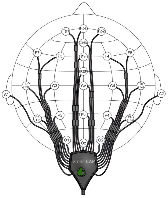
Figure 1.
Scheme of the EEG cap with Ag/AgCl sintered sensors by MCScap for the 24-channel SmartBCI wireless wearable EEG system.
In many researches, LCD monitors of personal computers are used as a solution for generating and presenting photostimuli to subjects. This approach has its disadvantages, such as the occurrence of harmonics in the EEG signal spectrum that are multiples of the screen refresh rate. Therefore, we used a special device of our own design, which provides a convenient process of generation and photostimuli presentation with a specified duration and frequency. More details about the device and its characteristics will be described in the following section.
Throughout the experiment, each subject was seated in a comfortable chair in a relaxed state. The room where the recording was performed was shaded to reduce interference from strong light. During the registration process for each subject, we carefully controlled the impedance values, which on average lay in the range of 4 to 7 kOhm. After the electrode placement procedure was completed, each subject was given 5 min to rest, and then the process of EEG data recording began. Before the photostimuli presentation, a 60 s fragment of the EEG signal in an eyes-closed state was recorded for each subject. The corresponding EEG signal fragments were marked with special labels in the EEG recording software. After this stage, the process of presenting photostimuli of given frequencies began.
In our study, we used a range of photostimulus frequencies from 5 to 25 Hz with steps of 1 Hz. Stimulation at each frequency was performed for 60 s. Each fragment of the EEG signal during the presentation of the photostimulus was marked with appropriate labels. During stimulation, participants were required to focus their attention on the flashes. They were also allowed to blink as needed. After each photostimuli presentation, participants were given 2–3 min to rest. An obligatory stage during each rest period involved verbal questioning of the participants about their well-being and discomfort experienced during the stimulation. Since none of the participants experienced discomfort, the survey data were not used in further analysis. Sufficient resting time was provided between stimulations to prevent visual fatigue. Thus, for each participant, a .xdf file was recorded, containing EEG signals from 21 channels, along with an additional signal from our photostimuli presentation device. Each file had an average duration of approximately one and a half hours.
5.1.3. The Photostimulation Device
Many researchers and developers of BCI systems use personal computer displays as sources of photostimuli. This imposes certain special requirements for the display. However, it is still possible for additional frequency components to occur, which could be a result of the screen refresh rate [54]. At the same time, in order to carry out research in this area, it makes sense, in the first approximation, to give preference to a special device that generates frequency-stable photostimuli, and is compatible with most of the EEG signal registration equipment.
While exploring the available EEG equipment markets, we encountered a challenge in finding photostimulators that were compatible with most manufacturers of EEG equipment and also offered the ability to finely adjust the frequency and duration of photostimuli. As a result, we created our own photostimulator with all the necessary characteristics and functionalities, as shown in Figure 2.
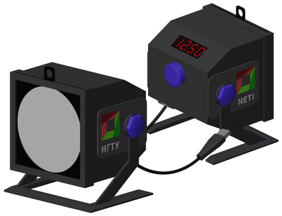
Figure 2.
The model of the developed photostimulator used for generating photostimuli in this study.
This device was based on an ATmega328P microcontroller with a maximum clock frequency of 20 MHz, which is more than sufficient for generating visible stimulations across the entire frequency range of interest. We utilized a 3D printer and additive technologies to produce the case and detachable elements (such as the stand, diffusing plates, and pattern-changing stencils) using PLA plastic.
The photostimulator described is equipped with an LED matrix consisting of 60 white light LEDs. This matrix serves as the source of light emissions for generating flashes during photostimulation. The device is capable of generating photostimuli with a specified frequency ranging from 0.5 to 60 Hz, with an increment value of 0.25 Hz. Additionally, it can produce photostimuli with durations ranging from 1 to 90 s, with an incremental value of 0.5 s.
To ensure uniform illumination, the photostimulator is equipped with a set of diffusing plates made of white PLA plastic, with a maximum diffusing surface area of 10 cm2. These plates have varying thicknesses (ranging from 0.3 mm to 2.0 mm), which help in achieving consistent and evenly distributed light output.
During the process of generating photostimuli, the stimulator’s specialized software takes control and generates an auxiliary signal. This signal is of rectangular shape and has a frequency equal to the frequency of the photostimulus being produced. The amplitude of this auxiliary signal is also set equal to the frequency of the photostimulus. This auxiliary signal is streamed using the lab-streaming layer protocol, allowing it to be recorded in parallel with the EEG signal. This simultaneous recording enables accurate detection of specific fragments within the EEG signal that coincide with the photostimulation events.
5.2. Pre-Processing and Descriptive Statistics
After obtaining the records from all participants, we used the MATLAB software package, version r2022b, for technical computing tasks. We utilized a band-pass filter with a bandwidth frequency range of 3 to 49 Hz to preprocess the EEG signals. Despite the fact that the occipital electrodes used in our calculations showed less prominent artifacts, such as EOG artifacts compared to frontal electrodes [53], we filtered out any activity in the frequency range up to 3 Hz. Additionally, due to the functioning of the notch filter used during the recording stage of the EEG signals, the frequency range of 45–55 Hz was unsuitable for our calculations; therefore, we suppressed all frequencies above 49 Hz.
Then, for each of the channels of occipital leads O1, O2, and Oz, we performed a procedure of extracting fragments of the EEG signal with photostimulation. Each fragment consisted of a 10 s interval before the presentation of the photostimulus, a 60 s fragment recorded during the presentation of the photostimulus, and a 20 s fragment after the end of the presentation of the photostimulus. Thus, for each participant, we obtained 21 × 3 EEG signal fragments of 90 s each. We carefully checked all obtained fragments for the absence of any artifacts that would prevent further computations. Finally, for each fragment, we calculated all the coefficients described in Section 4.
Thus, Figure 3 represents the dependence of the reaction speed coefficient on the photostimuli frequency for subject 3. This chart is presented for the fundamental and second harmonics of the stimulation frequencies for all occipital leads. It is important to note that, in our case, due to the effect of the notch filter, the results of calculating the second harmonic coefficients for frequencies beginning from 45 to 55 Hz do not provide any useful information and are not taken into account by us, since this frequency range was affected by the filter.
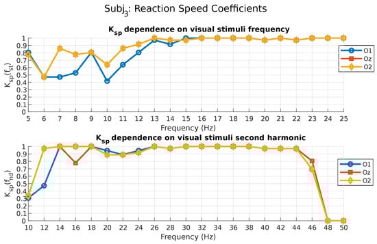
Figure 3.
Reaction speed coefficient values for subject 3.
As can be seen from the figure above, subject 3 demonstrates the best response speed (close to one) for photostimuli frequencies from 13 to 25 Hz, according to the coefficients calculated for the fundamental and second (excluding 23 Hz and above) harmonics (O2 and Oz leads). It can also be noted that for the coefficient, calculated for the second harmonic, photostimuli frequencies from 6 to 9 Hz can also be characterized as good in terms of the speed of response (O2 lead). For this subject it can be seen only for the second harmonic, but not for the fundamental. This once again emphasizes the importance of considering the response at multiples of frequencies. Table 1 and Table 2 present the results of calculating the coefficient in the Oz lead for all subjects who participated in the experiment.

Table 1.
coefficients at fundamental photostimuli frequencies, lead Oz.
Table 2.
coefficients at second harmonic photostimuli frequencies, lead Oz.
As can be seen from the data presented in Table 1 and Table 2, each subject’s reaction speed is highly individualized. Thus, subject 7 demonstrates extremely high coefficient values at all presented photostimulus frequencies for both the fundamental and second harmonics. In contrast, subject 6 showed some of the worst results, up to a complete absence of response at the fundamental (Table 1, frequencies 6, 10, and 11 Hz) and second (Table 2, frequencies 10, 16, 18, and 20 Hz) harmonics. This once again emphasizes the need for an individual approach to each user when selecting stimulation frequencies in BCIs.
Figure 4 represents the dependence of the threshold, overcoming coefficient on the photostimuli frequency for subject 3. This chart is presented for the fundamental and second harmonics of the stimulation frequencies for all occipital leads.
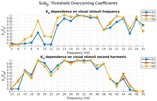
Figure 4.
Threshold overcoming coefficient values for subject 3.
As can be seen from the figure above, subject 3 demonstrated the most stable threshold overcoming response at photostimuli frequencies from 13 to 18 Hz, as well as at 21 and 24 Hz, according to the coefficient, calculated for the fundamental frequency (O2 and Oz leads). Although the level of his response in terms of the reaction criterion at the fundamental frequency was high enough from the stimulus frequency of 13 Hz to 25 Hz (Figure 3), the coefficient showed that not all of these photostimulus frequencies were able to produce a response. It can also be noted that while the coefficient, calculated for the second harmonic, (Figure 3) identified photostimuli frequencies from 6 to 9 Hz as acceptable in terms of reaction , the coefficient showed that only the stimulus frequency at 9 Hz from the mentioned range was able to produce a response at the second harmonic of photostimulus (O1, O2, and Oz leads). This example demonstrates that if one photostimulus frequency may be acceptable under one criterion, it does not mean that it will be acceptable under another criterion.
Table 3 and Table 4 contain the results of calculating the coefficient in the Oz lead for all subjects who participated in the experiment.
Table 3.
coefficients at fundamental photostimuli frequencies, lead Oz.
Table 4.
coefficients at the second harmonic photostimuli frequencies, lead Oz.
An analysis of the data presented in Table 3 and Table 4 also demonstrates the highly individual stability of the SSVEP potential response level caused by the photostimuli presentation. Thus, whereas subject 7 previously demonstrated an extremely high value of the coefficient over the entire frequency range (Table 1 and Table 2), in this case, the 5 and 6 Hz photostimulus frequencies do not exhibit as consistent a response level as the subsequent frequencies for which the coefficient was calculated at the fundamental frequency (Table 3). This subject was also characterized by a significant decrease in the coefficient calculated for the second harmonic from the photostimulus frequency of 16 Hz (32 Hz in Table 4) to 20 Hz, as well as to 22 and 23 Hz. At the same time, for subject 6, who demonstrates an extremely low speed of response (Table 1 and Table 2), the results obtained for the coefficient values remain very low, except for the 13–16 Hz photostimulus frequencies for the coefficient calculated at the fundamental frequency and the 22 Hz photostimulus frequency for the coefficient calculated for the second harmonic (44 Hz in Table 4).
The results of calculating the coefficient for subject 3 are shown in Figure 5. According to the coefficient formula (Equation (5)), the values close to one correspond to the photostimuli frequencies that evoke the fastest and most stable SSVEP potentials. Thus, this coefficient integrates both and coefficients and provides an indication of the frequency optimality according to two criteria at once.
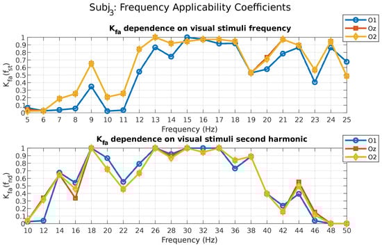
Figure 5.
Frequency applicability coefficient values for subject 3.
Thus, in the case of subject 3, the photostimuli frequencies at 13, 15–18, 21, and 24 Hz correspond to high-enough (at least 0.95) values of the coefficient , calculated for the fundamental frequency (O2 and Oz leads). At the same time, for the coefficient calculated for the second harmonic, the photostimuli frequencies of 9, 13, 15, and 17 Hz correspond to values exactly equal to one (O1, O2, and Oz leads). It should be noted that for this participant, the photostimulus frequencies of 13, 15, and 17 Hz have maximum values of the coefficient at the second harmonic. This further validates the relevance of evaluating the response not only at the fundamental frequency but also at its harmonics.
Table 5.
coefficients at fundamental photostimuli frequencies, lead Oz.
Table 6.
coefficients at second harmonic photostimuli frequencies, lead Oz.
Due to the fact that the coefficient takes into account both and coefficients, it can be used as an indicator of frequency optimality in terms of response speed and stability. For example, subject 7 demonstrated equal-to-one values for the coefficient calculated for fundamental frequency (Table 5) in the photostimuli frequency range from 7 to 24 Hz because of high values for (Table 1) and (Table 3) coefficients. Similar values of the coefficient calculated for the second harmonic are achieved for this subject in the first half of the used frequency range (Table 6). Analyzing the coefficient values for subject 3, who previously demonstrated very low values of (Table 1 and Table 2) and (Table 3 and Table 4) coefficients, the corresponding results can be seen. Thus, according to Table 5, the subject only has 3 values of the coefficient calculated for the fundamental frequency, namely, for 13, 15, and 16 Hz, which are close enough to one. The result of the calculation of the coefficient at the second harmonic in the case of the photostimulus frequency of 22 Hz (44 Hz in Table 6) can also be considered acceptable. These results suggest an extremely low ability of this subject to produce fast and stable SSVEP potentials, although this claim remains to be verified in practice. Nevertheless, even in this case, there were frequencies considered to be optimal, and one of them only corresponded to the second harmonic. This demonstrates that, by taking subharmonics into account, the frequency range used by the subject can theoretically be extended when the response at the fundamental frequency is too low or absent.
The values of the coefficient calculated for the fundamental and second harmonics can be averaged to obtain an even more strict value of the coefficient, since it equally accounts for the results achieved at the fundamental and multiple harmonics of a particular photostimulus frequency. The results of calculating the mean value of the coefficients for the fundamental and second harmonics are shown in Figure 6 for subject 3.
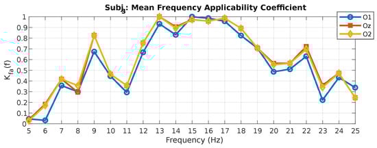
Figure 6.
Mean frequency applicability coefficient values for subject 3.
According to the values of this coefficient, we can assess which photostimuli frequencies are capable of producing the fastest and most stable SSVEP potentials on both the fundamental and second harmonics simultaneously. Thus, for subject 3, these are photostimuli with frequencies of 13 (O2 and Oz leads), 15–16 (O1 lead), and 17 (O2 and Oz leads) Hz. The results of calculating this coefficient for the remaining subjects are presented in Table 7.
Table 7.
Mean coefficients at photostimuli frequencies, lead Oz.
Based on Table 7, the most optimal (exactly equal to one) frequencies for subject 7, who demonstrates the best results among all participants in terms of the and coefficients, are the photostimuli frequencies of 7–10 Hz and 12 Hz. At the same time, the subject still has enough numbers of the averaged coefficient , as close to one as possible, namely, for the photostimuli frequencies 11, 13, 15, and 21 Hz. Subject 3, on the other hand, did not show any photostimulus frequency that could be recognized as optimal in terms of this coefficient because the maximum values of the coefficients for the fundamental and second harmonics did not overlap with each other in the frequency range (Table 5 and Table 6).
Additionally, as mentioned above, for each of the participants involved in the experiment, and for each stimulation frequency, we calculated the theta–beta ratio. This ratio is considered in the context of this study as an indicator of subjective stress or discomfort experienced during prolonged stimulation at a specific frequency. Individual values of these calculated ratios are presented in Table 8.
Table 8.
Theta–beta ratio.
The analysis of the obtained data revealed that the mean value of the index for the entire sample was 6.09 (SD = 3.54) during stimulation session and 5.47 (SD = 4.14) during the resting state with eyes closed. These data, among other things, indicate high values of inter-subject variability of the measured index. When examining the plot of the index values for individual frequencies, a noticeable decline in theta–beta ratio scores is observed for males at frequencies of 20–21 Hz, with a tendency to return to average values with further increases in stimulation frequency (Figure 7). The overall downward trend of the obtained values may indicate a decrease in discomfort when transitioning from a low- to high-frequency stimulation, which is consistent with existing literature data [21]. Conducting a more detailed statistical analysis across groups that differ in terms of gender or stimulation frequency is challenging due to the small sample size within this pilot study.
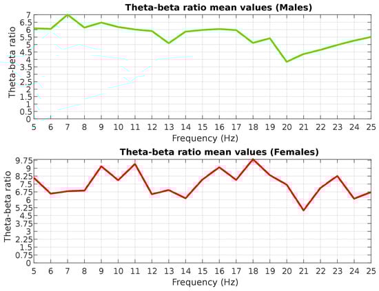
Figure 7.
Average theta–beta ratio for males and females.
The resulting theta–beta ratios are then normalized to a range of 0 to 1 according to Equation (8) to obtain a discomfort coefficient . An example of such normalization for subject 3 is shown in Figure 8.
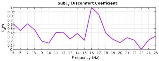
Figure 8.
Discomfort coefficient values for subject 3.
The values of this coefficient can additionally be used to filter out some of the optimal frequencies selected by the values of the coefficients, although it should be noted that they are highly empirical in nature, and the same value of this coefficient can mean a completely different level of discomfort for different subjects.
5.3. Coefficients Analysis Application
We used the C++ programming language and the Qt library version 5.14 to create an application with a graphical user interface. With the help of this application, it is possible to analyze the calculated coefficients and generate a list of optimal photostimuli frequencies for each subject. The app’s appearance is shown in Figure 9.
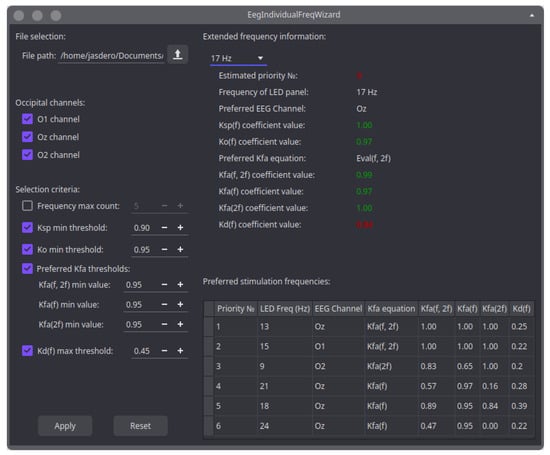
Figure 9.
Main window of the developed application.
This application consists of two sections. In the first section, located on the left, the user specifies the necessary input data used for analyzing the coefficients and generating a list of recommended stimulation frequencies. In the second section, located on the right, the user can view the results of the coefficient analysis performed according to the input parameters specified by them. Thus, in the upper part of this section, the user can view detailed information about any stimulation frequency for which coefficients have been calculated. In particular, this will allow the user to find out which criteria led to the exclusion of a particular frequency from the recommended list. The corresponding values that did not pass any criteria are colored in red. In the lower part of this section, there is a final list of recommended frequencies presented in the form of a table. Each row of the table is sorted in descending order of the stimulation frequency rating.
When starting to use the application, it is necessary to specify the path to the file with the coefficients calculated in MATLAB for each stimulation frequency (in the left part of the application). Then, the user must provide a set of criteria for selecting stimulation frequencies in the corresponding sections. The list of selection criteria available for setting was chosen in such a way that the user can adapt the behavior of the application to their goals and tasks. For example, the user can specify occipital leads for which the coefficient analysis needs to be performed. We added this feature to the application for the reason that a subject’s individual response to the presented frequencies may appear not only in the reaction level of the occurring SSVEP potential but also in the location of this response among the occipital electrodes. For example, in the previous section, in the phase of calculating the basic coefficients for subject 3, the vast majority of optimal coefficients were at the O2 and Oz electrodes, while the values for the O1 electrode were lower. However, this is not a strict rule and is highly dependent on subject differences. Thus, even in the case of subject 3, an example can be given where the highest response was found on electrode O1; it can be seen in Figure 5 for photostimulus frequencies of 15 Hz (for the coefficient calculated for the fundamental frequency) and 16 Hz (for the coefficient calculated for the second harmonic). This allows for determining the rating of each frequency and identifying the most suitable EEG channel for searching for SSVEP potential at any stimulation frequency. If necessary, the user can specify the exact number of frequencies recommended by the application, depending on the requirements of the BCI, or leave this section disabled to turn off the frequency number limitation. In the following sections, the user needs to set the minimum permissible threshold values for the and coefficients proposed in this article.
Establishing minimum acceptable thresholds for these coefficients provides fine control over how the application prioritizes certain frequencies. For example, setting the coefficient threshold closer to one and decreasing the coefficient threshold will cause the application to prioritize stimulation frequencies with the most stable threshold overshoot of SNR. And if the user needs the fastest response to a stimulus, then it is possible to set the coefficient threshold close to one, and slightly decrease the coefficient threshold. In cases where there are strict requirements for response speed and SNR threshold overshoot, both thresholds of these coefficients can be set closer to one, although this may significantly reduce the final list of recommended frequencies.
The application also includes the ability to set minimum values for the three coefficients. The proximity of these coefficients to one depends heavily on the values of the and coefficients. Therefore, setting the minimum allowable values for the coefficients ensures that the mutual influence of the and coefficients will not result in the application selecting a frequency with a maximum value for one coefficient at the expense of significantly reducing the other. Instead, the application will maintain a balance between the values of the and coefficients by selecting stimulation frequencies that best satisfy the established thresholds for the , , and coefficients simultaneously. In this case, only the threshold coefficient with the maximum value will be considered for each photostimulus frequency. As a result, the list of recommended frequencies will also indicate which coefficient formula should be used to detect SSVEP potential at a given photostimulus frequency. This allows us to additionally consider stimulation frequencies where the SSVEP potential is exclusively present at the main or multiple stimulation frequencies. Additionally, this approach takes into account different time delays or response stabilities at the main and multiple frequencies, selecting the best option. Considering these factors expands the final list of recommended frequencies.
The process of selecting recommended frequencies in our application was designed in such a way that the first priority is given to searching for stimulation frequencies that exceed the threshold value of the coefficient. This ensures that the list primarily includes frequencies that produce a high response at both the main and multiple stimulation frequencies. The remaining frequencies are then selected in descending order of the values of the and coefficients, which are analyzed as a unified list. This approach allows us to properly take into account those subjects who are most characterized by SSVEP potentials occurring at multiple stimulation frequencies rather than at the main stimulation frequencies.
Finally, the user can set the maximum allowable discomfort coefficient as the last threshold value. This allows the list of recommended frequencies to be adjusted by excluding frequencies that cause discomfort for the subject. For example, as shown in Figure 9, our application excluded the frequency of photostimulation at 17 Hz from the list of recommended frequencies due to its high discomfort coefficient. However, this frequency passed all other threshold values set for the , , and coefficients.
It is important to note that because SSVEP potentials can arise not just at the primary frequency but also at its multiples, some chosen frequencies might be mathematically incompatible. For example, the photostimuli presentation with a frequency of 5 and 10 Hz in both cases can provoke a reaction at 10 Hz, 20 Hz, etc. This feature is not taken into account in our application because its primary goal is to generate the most complete list of potentially usable frequencies.
6. Discussion
In this study, to determine individual stimulation frequencies, we used criteria such as the reaction onset speed in response to presented visual stimuli, the capacity to maintain a consistent response at an acceptable level during continuous visual stimuli presentation, and user satisfaction with the presented photostimulus to identify individual stimulation frequencies. For this purpose, we proposed a number of coefficients based on the SNR and theta-to-beta power ratio:
- Reaction reaction speed coefficient ;
- Threshold overcoming coefficient ;
- Frequency applicability coefficient ;
- Discomfort coefficient .
Each coefficient serves as a quantitative measure, ranging from 0 to 1, which characterizes the extent to which the stimulation frequency is suitable for the subject in terms of various factors, including the response onset speed to the presented photostimuli, the stability of the response, the overall applicability of the frequency, and the level of induced stress. Notably, our study utilized these coefficients to account for subject responses, not only at the fundamental frequency but also at the second harmonic of the photostimulus frequency. This approach enabled the identification of frequencies that may have elicited weak responses at the fundamental frequency but demonstrated favorable outcomes at the second harmonic.
The results of calculating these coefficients in Section 5.2 demonstrate the highly individualized response of each subject to the presented photostimuli.
To facilitate working with the obtained coefficients, we developed a special application described in Section 5.3. With the help of this application, the user can adjust the desired threshold values of the calculated coefficients and automatically obtain a set of photostimulus frequencies most appropriate for a particular subject.
During the course of this study, notable variations in SSVEP response were observed among subjects. In certain instances, the reaction was indistinguishable, while in others, the reaction was only significant on the fundamental frequency or subharmonic frequency. These findings indicate that an individualized approach may be necessary, as certain frequencies may not be suitable for all patients, but this does not preclude the possibility of other frequencies being effective. Additionally, some subjects exhibited more pronounced responses to subharmonics, suggesting that incorporating subharmonics into SSVEP may enhance the accessibility of SSVEP-BCI.
It is crucial to situate the findings of our study within the broader context of previous studies and obtain results. For example, in the study by Kus et al., the researchers aimed to determine the SSVEP response curve, which represented the magnitude of the evoked signal based on frequency. They induced the SSVEP response using a wide range of frequencies (5–30 Hz) and collected data from 10 subjects. The main finding of the study was the identification of the optimal frequency range (12–18 Hz) for detecting SSVEP [31]. The authors of another relevant paper successfully used a filter bank canonical correlation analysis to incorporate fundamental and harmonic frequency components to improve the detection of SSVEPs [55]. In line with these findings, the results of our study point to the same range for optimal stimulation frequencies, encompassing high alpha and low beta EEG frequency bands. However, within this optimal range, different subjects have their own most suitable frequencies at which the speed and stability of the evoked SSVEP potential are high enough. Furthermore, we demonstrated that considering not only the fundamental frequency of the photostimulation but also the second harmonic frequency improved the estimation of the reaction onset rate and stability of the SSVEP response. This approach enabled us to account for individual user characteristics and extend the frequency range, particularly in the low-frequency range, where the signal-to-noise ratio may be compromised.
As a limitation of the methodology for individual frequency selection in general, it is important to note that the individual calibration process might need to be repeated after a while, since the human body is prone to changes, especially over longer periods of time (months and years). And, indeed, the individual reactions might be different due to a user’s condition. However, this deserves a specific study and is beyond the scope of our current paper. It is also important to note that some frequencies may be mathematically incompatible. For example, if a 5 Hz photostimulus does not evoke a response at the fundamental but at the second (10 Hz) harmonic, then such a photostimulus may be indistinguishable from a 10 Hz stimulation frequency, which evokes a response only at the fundamental frequency. However, this fact is more of a limitation of the SSVEP paradigm itself than of our proposed method.
7. Conclusions
Brain–computer interfaces are rapidly gaining popularity due to their potentially wide range of applications, being equally beneficial for both healthy individuals and patients suffering from severe illnesses. The vast number of approaches, relying on various neurophysiological mechanisms and methods of acquisition and processing, provides an opportunity to actively pursue multiple directions in search of optimal solutions. One such approach that has demonstrated practical effectiveness involves the development of BCIs based on steady-state visually evoked potential. Currently used stimulation protocols typically focus on frequencies exceeding 30 Hz, which is attributed to lower fatigue likelihood in individuals as well as reduced probability of epileptic activity when displaying rhythmically flickering stimuli. However, within the scope of this current research, we focused on a frequency range from 5 to 25 Hz. The use of photoflashes at these frequencies yields a maximum SSVEP amplitude compared to frequencies above 30 Hz [13]. By limiting ourselves to frequencies within this range, our objective was to develop an algorithm for identifying the most optimal stimulation frequencies for each subject while considering their subjective level of stress/discomfort (being quantified by using the theta-to-beta power ratio) when presented with stimuli at specific frequencies.
The improvement of approaches in developing increasingly reliable, accurate, and user-friendly brain–computer interfaces enables the active integration of these technologies into clinical practice, significantly enhancing the quality of life for patients. Over the decades of BCI utilization, including those based on SSVEP, substantial advancements have been achieved in rehabilitating patients who have suffered from strokes [56,57], as well as patients recovering from severe spinal [58] or brain injuries [59,60]. Personalization of diagnostic programs and therapeutic interventions in modern medicine is one of the main directions of development. The development of next-generation interfaces that take into account a greater number of influencing factors, considering the individual condition of the patient during BCI training, will potentially provide patients with the ability to actively interact with the external world and lead lifestyles that are qualitatively indistinguishable from those of healthy individuals. Despite being conducted on a sample of healthy subjects, our study nevertheless has the feasibility and potential to be used on patients who are experiencing significant difficulties in returning to their normal lives after a previous illness.
Future plans include performing the experiment described in this article on a larger group of participants, using the obtained individual stimulation frequencies in real conditions, and analyzing the variability of optimal frequencies calculated for participants over time. We also plan to quantitatively evaluate the reasonability of this approach relative to other methods for selecting individual photostimuli frequencies and the scenario without any selection at all.
Author Contributions
Conceptualization, A.K., A.G., M.B., A.P. and O.R.; methodology, A.K. and A.G.; software, A.K.; validation, A.K., A.G. and M.B.; formal analysis, A.K., A.G. and A.P.; investigation, A.K. and A.G.; resources, A.K.; data curation, A.K.; writing—original draft preparation, A.K., A.G., M.B. and A.P.; writing—review and editing, O.R.; visualization, A.K.; supervision, O.R.; project administration, M.B.; funding acquisition, M.B. All authors have read and agreed to the published version of the manuscript.
Funding
This research received no external funding.
Institutional Review Board Statement
The study was conducted according to the guidelines of the Declaration of Helsinki and approved by the Ethics Committee of the Faculty of Humanities of Novosibirsk State Technical University (protocol code 01_02_2023).
Data Availability Statement
The data presented in this study are available upon request from the corresponding author.
Acknowledgments
We would like to thank all the volunteers who took part in the experimental sessions. Their participation provided valuable data that can be used for further research and the development of new approaches in this area.
Conflicts of Interest
The authors declare no conflict of interest.
Abbreviations
The following abbreviations are used in this manuscript:
| AI | artificial intelligence |
| BCI | brain–computer interface |
| DI | discomfort index |
| ECoG | electrocorticography |
| EEG | electroencephalography |
| EOG | electrooculography |
| FFT | fast Fourier transform |
| GUI | graphical user interface |
| ITR | information transfer rate |
| LD | linear dichroism |
| MDPI | Multidisciplinary Digital Publishing Institute |
| SD | standard deviation |
| SNR | signal-to-noise ratio |
| SSVEP | steady-state visually evoked potential |
| UI | user interface |
| UX | user experience |
References
- Khademi, Z.; Ebrahimi, F.; Kordy, H.M. A review of critical challenges in MI-BCI: From conventional to deep learning methods. J. Neurosci. Methods 2023, 383, 109736. [Google Scholar] [CrossRef] [PubMed]
- Zgallai, W.; Brown, J.T.; Ibrahim, A.; Mahmood, F.; Mohammad, K.; Khalfan, M.; Mohammed, M.; Salem, M.; Hamood, N. Deep learning AI application to an EEG driven BCI smart wheelchair. In Proceedings of the 2019 Advances in Science and Engineering Technology International Conferences (ASET), Dubai, United Arab Emirates, 26 March–10 April 2019; pp. 1–5. [Google Scholar]
- Dehais, F.; Dupres, A.; Di Flumeri, G.; Verdiere, K.; Borghini, G.; Babiloni, F.; Roy, R. Monitoring pilot’s cognitive fatigue with engagement features in simulated and actual flight conditions using an hybrid fNIRS-EEG passive BCI. In Proceedings of the 2018 IEEE International Conference on Systems, Man, and Cybernetics (SMC), Miyazaki, Japan, 7–10 October 2018; pp. 544–549. [Google Scholar]
- Zander, T.O.; Kothe, C.; Jatzev, S.; Gaertner, M. Enhancing human-computer interaction with input from active and passive brain-computer interfaces. In Brain-Computer Interfaces: Applying our Minds to Human-Computer Interaction; Springer: London, UK, 2010; pp. 181–199. [Google Scholar]
- Abiri, R.; Borhani, S.; Sellers, E.W.; Jiang, Y.; Zhao, X. A comprehensive review of EEG-based brain—Computer interface paradigms. J. Neural Eng. 2019, 16, 011001. [Google Scholar] [CrossRef] [PubMed]
- Xiao, X.; Wang, L.; Xu, M.; Wang, K.; Jung, T.P.; Ming, D. A data expansion technique based on training and testing sample to boost the detection of SSVEPs for brain-computer interfaces. J. Neural Eng. 2023. [Google Scholar] [CrossRef] [PubMed]
- Liu, S.; Zhang, D.; Liu, Z.; Liu, M.; Ming, Z.; Liu, T.; Suo, D.; Funahashi, S.; Yan, T. Review of brain—Computer interface based on steady-state visual evoked potential. Brain Sci. Adv. 2022, 8, 258–275. [Google Scholar] [CrossRef]
- Wittevrongel, B.; Khachatryan, E.; Hnazaee, M.F.; Carrette, E.; De Taeye, L.; Meurs, A.; Boon, P.; Van Roost, D.; Van Hulle, M.M. Representation of steady-state visual evoked potentials elicited by luminance flicker in human occipital cortex: An electrocorticography study. Neuroimage 2018, 175, 315–326. [Google Scholar] [CrossRef] [PubMed]
- Chen, X.; Wang, Y.; Nakanishi, M.; Gao, X.; Jung, T.P.; Gao, S. High-speed spelling with a noninvasive brain—Computer interface. Proc. Natl. Acad. Sci. USA 2015, 112, E6058–E6067. [Google Scholar] [CrossRef] [PubMed]
- Zhu, D.; Bieger, J.; Molina, G.G.; Aarts, R.M. A survey of stimulation methods used in SSVEP-based BCIs. Comput. Intell. Neurosci. 2010, 2010, 702357. [Google Scholar] [CrossRef]
- Wolpaw, J.; Ramoser, H.; McFarland, D.; Pfurtscheller, G. EEG-based communication: Improved accuracy by response verification. IEEE Trans. Rehabil. Eng. 1998, 6, 326–333. [Google Scholar] [CrossRef]
- Zhang, J.; Gao, S.; Zhou, K.; Cheng, Y.; Mao, S. An online hybrid BCI combining SSVEP and EOG-based eye movements. Front. Hum. Neurosci. 2023, 17, 1103935. [Google Scholar] [CrossRef]
- Won, D.; Hwang, H.; Dähne, S.; Müller, K.; Lee, S. Effect of higher frequency on the classification of steady-state visual evoked potentials. J. Neural Eng. 2015, 13, 016014. [Google Scholar] [CrossRef]
- Adams, M.; Benda, M.; Saboor, A.; Krause, A.F.; Rezeika, A.; Gembler, F.; Stawicki, P.; Hesse, M.; Essig, K.; Ben-Salem, S.; et al. Towards an SSVEP-BCI Controlled Smart Home. In Proceedings of the IEEE International Conference on Systems, Man and Cybernetics, Bari, Italy, 6–9 October 2019; Volume 1. [Google Scholar]
- Lesenfants, D.; Habbal, D.; Lugo, Z.; Lebeau, M.; Horki, P.; Amico, E.; Pokorny, C.; Gómez, F.; Soddu, A.; Müller-Putz, G.; et al. An independent SSVEP-based brain–computer interface in locked-in syndrome. J. Neural Eng. 2014, 11, 035002. [Google Scholar] [CrossRef] [PubMed]
- Na, R.; Hu, C.; Sun, Y.; Wang, S.; Zhang, S.; Han, M.; Yin, W.; Zhang, J.; Chen, X.; Zheng, D. An embedded lightweight SSVEP-BCI electric wheelchair with hybrid stimulator. Digit. Signal Process. 2021, 116, 103101. [Google Scholar] [CrossRef]
- Shi, N.; Li, X.; Liu, B.; Yang, C.; Wang, Y.; Gao, X. Representative-Based Cold Start for Adaptive SSVEP-BCI. IEEE Trans. Neural Syst. Rehabil. Eng. 2023, 31, 1521–1531. [Google Scholar] [CrossRef] [PubMed]
- Han, D.K.; Jeong, J.H. Domain generalization for session-independent brain-computer interface. In Proceedings of the 2021 9th International Winter Conference on Brain-Computer Interface (BCI), Gangwon, Republic of Korea, 22–24 February 2021; pp. 1–5. [Google Scholar]
- Li, J.; Wang, F.; Huang, H.; Qi, F.; Pan, J. A novel semi-supervised meta learning method for subject-transfer brain–computer interface. Neural Netw. 2023, 163, 195–204. [Google Scholar] [CrossRef] [PubMed]
- Li, M.; Xu, D. Transfer Learning in Motor Imagery Brain Computer Interface: A Review. J. Shanghai Jiaotong Univ. Sci. 2022, 1–23. [Google Scholar] [CrossRef]
- Ladouce, S.; Darmet, L.; Torre Tresols, J.J.; Velut, S.; Ferraro, G.; Dehais, F. Improving user experience of SSVEP BCI through low amplitude depth and high frequency stimuli design. Sci. Rep. 2022, 12, 8865. [Google Scholar] [CrossRef] [PubMed]
- Silva, L.C.B.; Kasteleijn-Nolst Trenite, D.; Manreza, M.L.; Appleton, R.E. Epidemiology of Sensitivity of the Brain to Intermittent Photic Stimulation and Patterns. In The Importance of Photosensitivity for Epilepsy; Springer: Cham, Switzerland, 2021; pp. 3–25. [Google Scholar]
- Zhang, H.Y.; Stevenson, C.E.; Jung, T.P.; Ko, L.W. Stress-Induced Effects in Resting EEG Spectra Predict the Performance of SSVEP-Based BCI. IEEE Trans. Neural Syst. Rehabil. Eng. 2020, 28, 1771–1780. [Google Scholar] [CrossRef] [PubMed]
- Putman, P.; Verkuil, B.; Arias-Garcia, E.; Pantazi, I.; van Schie, C. EEG theta/beta ratio as a potential biomarker for attentional control and resilience against deleterious effects of stress on attention. Cogn. Affect. Behav. Neurosci. 2014, 14, 782–791. [Google Scholar] [CrossRef]
- Vanhollebeke, G.; De Smet, S.; De Raedt, R.; Baeken, C.; van Mierlo, P.; Vanderhasselt, M.A. The neural correlates of psychosocial stress: A systematic review and meta-analysis of spectral analysis EEG studies. Neurobiol. Stress 2022, 18, 100452. [Google Scholar] [CrossRef]
- Goodman, R.N.; Rietschel, J.C.; Lo, L.C.; Costanzo, M.E.; Hatfield, B.D. Stress, emotion regulation and cognitive performance: The predictive contributions of trait and state relative frontal EEG alpha asymmetry. Int. J. Psychophysiol. 2013, 87, 115–123. [Google Scholar] [CrossRef]
- Nam, C.S. Brain–computer interface (BCI) and ergonomics. Ergonomics 2012, 55, 513–515. [Google Scholar] [CrossRef] [PubMed]
- Bos, D.P.O.; Reuderink, B.; van de Laar, B.; Gürkök, H.; Mühl, C.; Poel, M.; Heylen, D.; Nijholt, A. Human-computer interaction for BCI games: Usability and user experience. In Proceedings of the 2010 International Conference on Cyberworlds, Singapore, 20–22 October 2010; pp. 277–281. [Google Scholar]
- van de Laar, B.; Gürkök, H.; Plass-Oude Bos, D.; Nijboer, F.; Nijholt, A. Perspectives on user experience evaluation of brain-computer interfaces. In Proceedings of the Universal Access in Human-Computer Interaction, Users Diversity: 6th International Conference, UAHCI 2011, Held as Part of HCI International 2011, Orlando, FL, USA, 9–14 July 2011; Springer: Berlin/Heidelberg, Germany, 2011; pp. 600–609. [Google Scholar]
- Chailloux Peguero, J.D.; Hernández-Rojas, L.G.; Mendoza-Montoya, O.; Caraza, R.; Antelis, J.M. SSVEP detection assessment by combining visual stimuli paradigms and no-training detection methods. Front. Neurosci. 2023, 17, 1142892. [Google Scholar] [CrossRef] [PubMed]
- Kuś, R.; Duszyk, A.; Milanowski, P.; Łabęcki, M.; Bierzyńska, M.; Radzikowska, Z.; Michalska, M.; Żygierewicz, J.; Suffczyński, P.; Durka, P.J. On the Quantification of SSVEP Frequency Responses in Human EEG in Realistic BCI Conditions. PLoS ONE 2013, 8, e77536. [Google Scholar] [CrossRef]
- Ng, K.B.; Bradley, A.P.; Cunnington, R. Stimulus specificity of a steady-state visual-evoked potential-based brain–computer interface. J. Neural Eng. 2012, 9, 036008. [Google Scholar] [CrossRef] [PubMed]
- Wu, Y.; Yang, R.; Chen, W.; Li, X.; Niu, J. Research on Unsupervised Classification Algorithm Based on SSVEP. Appl. Sci. 2022, 12, 8274. [Google Scholar] [CrossRef]
- Kennedy, P.R.; Bakay, R.A.E. Restoration of neural output from a paralyzed patient by a direct brain connection. NeuroReport 1998, 9, 1707–1711. [Google Scholar] [CrossRef] [PubMed]
- Hochberg, L.R.; Serruya, M.D.; Friehs, G.M.; Mukand, J.A.; Saleh, M.; Caplan, A.H.; Branner, A.; Chen, D.; Penn, R.D.; Donoghue, J.P. Neuronal ensemble control of prosthetic devices by a human with tetraplegia. Nature 2006, 442, 164–171. [Google Scholar] [CrossRef] [PubMed]
- Défossez, A.; Caucheteux, C.; Rapin, J.; Kabeli, O.; King, J.R. Decoding speech perception from non-invasive brain recordings. Nat. Mach. Intell. 2023, 5, 1097–1107. [Google Scholar] [CrossRef]
- Orban, M.; Elsamanty, M.; Guo, K.; Zhang, S.; Yang, H. A Review of Brain Activity and EEG-Based Brain–Computer Interfaces for Rehabilitation Application. Bioengineering 2022, 9, 768. [Google Scholar] [CrossRef]
- Varone, G.; Boulila, W.; Driss, M.; Kumari, S.; Khan, M.K.; Gadekallu, T.R.; Hussain, A. Finger pinching and imagination classification: A fusion of CNN architectures for IoMT-enabled BCI applications. Inf. Fusion 2024, 101, 102006. [Google Scholar] [CrossRef]
- Aricò, P.; Borghini, G.; Di Flumeri, G.; Sciaraffa, N.; Babiloni, F. Passive BCI beyond the lab: Current trends and future directions. Physiol. Meas. 2018, 39, 08TR02. [Google Scholar] [CrossRef] [PubMed]
- Miller, K.J.; Hermes, D.; Staff, N.P. The current state of electrocorticography-based brain–computer interfaces. Neurosurg. Focus 2020, 49, E2. [Google Scholar] [CrossRef] [PubMed]
- Wong, C.M.; Wang, Z.; Nakanishi, M.; Wang, B.; Rosa, A.; Chen, C.P.; Jung, T.P.; Wan, F. Online adaptation boosts SSVEP-based BCI performance. IEEE Trans. Biomed. Eng. 2021, 69, 2018–2028. [Google Scholar] [CrossRef] [PubMed]
- Zerafa, R.; Camilleri, T.; Falzon, O.; Camilleri, K.P. To train or not to train? A survey on training of feature extraction methods for SSVEP-based BCIs. J. Neural Eng. 2018, 15, 051001. [Google Scholar] [CrossRef] [PubMed]
- Yao, L.; Jiang, N.; Mrachacz-Kersting, N.; Zhu, X.; Farina, D.; Wang, Y. Reducing the calibration time in somatosensory BCI by using tactile ERD. IEEE Trans. Neural Syst. Rehabil. Eng. 2022, 30, 1870–1876. [Google Scholar] [CrossRef] [PubMed]
- Holz, E.M.; Höhne, J.; Staiger-Sälzer, P.; Tangermann, M.; Kübler, A. Brain–computer interface controlled gaming: Evaluation of usability by severely motor restricted end-users. Artif. Intell. Med. 2013, 59, 111–120. [Google Scholar] [CrossRef] [PubMed]
- Ortega, Y.; Mezura-Godoy, C. Usability Evaluation of BCI Software Applications: A systematic review of the literature. Program. Comput. Softw. 2022, 48, 646–657. [Google Scholar] [CrossRef]
- Ming, G.; Pei, W.; Chen, H.; Gao, X.; Wang, Y. Optimizing spatial properties of a new checkerboard-like visual stimulus for user-friendly SSVEP-based BCIs. J. Neural Eng. 2021, 18, 056046. [Google Scholar] [CrossRef]
- Ming, G.; Pei, W.; Gao, X.; Wang, Y. A high-performance SSVEP-based BCI using imperceptible flickers. J. Neural Eng. 2023, 20, 016042. [Google Scholar] [CrossRef]
- Xu, D.; Tang, F.; Li, Y.; Zhang, Q.; Feng, X. An Analysis of Deep Learning Models in SSVEP-Based BCI: A Survey. Brain Sci. 2023, 13, 483. [Google Scholar] [CrossRef]
- Davidov, A.; Razumnikova, O.; Bakaev, M. Nature in the Heart and Mind of the Beholder: Psycho-Emotional and EEG Differences in Perception of Virtual Nature Due to Gender. Vision 2023, 7, 30. [Google Scholar] [CrossRef]
- Putman, P.; van Peer, J.; Maimari, I.; van der Werff, S. EEG theta/beta ratio in relation to fear-modulated response-inhibition, attentional control, and affective traits. Biol. Psychol. 2010, 83, 73–78. [Google Scholar] [CrossRef] [PubMed]
- Altaf, H.; Ibrahim, S.N.; Azmin, N.; Asnawi, A.L.; Walid, B.H.B.; Harun, N. Machine Learning Approach for Stress Detection based on Alpha-Beta and Theta-Beta Ratios of EEG Signals. In Proceedings of the 2021 13th International Conference on Information & Communication Technology and System (ICTS), Surabaya, Indonesia, 20–21 October 2021; pp. 201–206. [Google Scholar]
- Schutter, D.J.L.G.; Kenemans, J.L. Theta-Beta Power Ratio: An Electrophysiological Signature of Motivation, Attention and Cognitive Control; Oxford University Press: Oxford, UK, 2022. [Google Scholar]
- Jiang, X.; Bian, G.B.; Tian, Z. Removal of Artifacts from EEG Signals: A Review. Sensors 2019, 19, 987. [Google Scholar] [CrossRef]
- Chen, X.; Liu, B.; Wang, Y.; Cui, H.; Dong, J.; Ma, R.; Li, N.; Ga, X. Optimizing Stimulus Frequency Ranges for Building a High-Rate High Frequency SSVEP-BCI. IEEE Trans. Neural Syst. Rehabil. Eng. 2023, 31, 1277–1286. [Google Scholar] [CrossRef]
- Chen, X.; Wang, Y.; Gao, S.; Jung, T.P.; Gao, X. Filter bank canonical correlation analysis for implementing a high-speed SSVEP-based brain–computer interface. J. Neural Eng. 2015, 12, 046008. [Google Scholar] [CrossRef] [PubMed]
- Guo, N.; Wang, X.; Duanmu, D.; Huang, X.; Li, X.; Fan, Y.; Li, H.; Liu, Y.; Yeung, E.H.K.; To, M.K.T.; et al. SSVEP-Based Brain Computer Interface Controlled Soft Robotic Glove for Post-Stroke Hand Function Rehabilitation. IEEE Trans. Neural Syst. Rehabil. Eng. 2022, 30, 1737–1744. [Google Scholar] [CrossRef] [PubMed]
- Bamdad, M.; Zarshenas, H.; Auais, M.A. Application of BCI systems in neurorehabilitation: A scoping review. Disabil. Rehabil. Assist. Technol. 2013, 10, 355–364. [Google Scholar] [CrossRef]
- Rupp, R. Challenges in clinical applications of brain computer interfaces in individuals with spinal cord injury. Front. Neuroeng. 2014, 7, 38. [Google Scholar] [CrossRef]
- Pan, J.; Xie, Q.; Qin, P.; Chen, Y.; He, Y.; Huang, H.; Wang, F.; Ni, X.; Cichocki, A.; Yu, R.; et al. Prognosis for patients with cognitive motor dissociation identified by brain-computer interface. Brain 2020, 143, 1177–1189. [Google Scholar] [CrossRef]
- Brennan, C.; McCullagh, P.; Lightbody, G.; Galway, L.; McClean, S.; Stawicki, P.; Gembler, F.; Volosyak, I.; Armstrong, E.; Thompson, E. Performance of a Steady-State Visual Evoked Potential and Eye Gaze Hybrid Brain-Computer Interface on Participants with and without a Brain Injury. IEEE Trans. Hum.-Mach. Syst. 2020, 50, 277–286. [Google Scholar] [CrossRef]
Disclaimer/Publisher’s Note: The statements, opinions and data contained in all publications are solely those of the individual author(s) and contributor(s) and not of MDPI and/or the editor(s). MDPI and/or the editor(s) disclaim responsibility for any injury to people or property resulting from any ideas, methods, instructions or products referred to in the content. |
© 2023 by the authors. Licensee MDPI, Basel, Switzerland. This article is an open access article distributed under the terms and conditions of the Creative Commons Attribution (CC BY) license (https://creativecommons.org/licenses/by/4.0/).