Indoor Comfort and Energy Consumption Optimization Using an Inertia Weight Artificial Bee Colony Algorithm

Abstract

A comfortable indoor environment contributes to a better quality of life and wellbeing for its occupants. The indoor temperature, lighting, and air quality are the main controlling factors of user comfort levels. The optimum control of the lighting, air conditioners, and air ventilators helps in maximizing the user’s comfort level. Nonetheless, the energy consumption of these appliances needs to be taken into consideration to minimize the operational cost and at the same time provide an environmentally friendly system. Comfort level maximization and energy consumption minimization are optimization problems. This issue is becoming more important due to the lifestyle changes caused by the COVID-19 pandemic that resulted in more time spent at home and indoors. Inertia weight artificial bee colony (IW-ABC) algorithms using linearly increasing, linearly decreasing, and exponentially increasing inertia are proposed here for the optimization of the indoor comfort index and energy usage. The multi-objective problem is tackled as a weighted single objective optimization problem. The proposed solution is tested using a dataset of 48 environmental conditions. The results of the simulation show that the IW-ABC performs better than the original ABC and other benchmark algorithms and the IW-ABC with linear increasing inertia weight has the most improved convergence behavior.

1. Introduction

The global population spends most of its time indoors, with a higher percentage at home than any other premises. Americans were reported to spend more than 65% of their time at home [1], while New Zealander and Canadian adults spend 60–70% at home [2].

The outbreak of the COVID-19 pandemic late in 2019 caused the “stay at home” campaign to grow into a worldwide phenomenon as an effort to combat the pandemic and break chains of transmission. Lockdown, social distancing, and movement control orders are enforced in many countries, while remote working specifically from home is now the new norm. This further increases the amount of time we spend indoors at home. The Google COVID-19 Community Report (https://www.google.com/covid19/mobility/, accessed on 1 August 2022) data up to 5 October 2022 show an increase of time spent at home for most countries, with a rise of +4% observed in the United State and Canada, +6% in the United Kingdom and New Zealand, +9% in Malaysia, and +10% in Singapore. Additionally, time spent in the workplace is declining up to −26% in these countries. At the height of the pandemic, venturing outdoors was allowed only for absolute necessary reasons such as for medical appointments. Most social and leisure activities were restricted in efforts to reduce the risks of close contacts and exposure to the virus. This abrupt change of lifestyle caused a rise in mental health issues due to loneliness, lack of physical and social interaction, anxiety due to changes in daily life, and many other reasons [3,4]. These mental health issues are part of the domino effects of COVID-19. However, life is now getting back to normalcy, though some of the policies adopted during the height of the COVID-19 outbreak are anticipated to be maintained, particularly remote working. Employers and employees are responding positively toward the continuation of this arrangement even after the pandemic [5,6].

Providing a comfortable indoor environment helps in improving productivity for the occupants [7] and also helps the occupants’ physical and mental health [8]. Therefore, ensuring a pleasant and comfortable indoor environment is important. The indoor temperature, illumination, and air quality are known to be the major parameters that affect an occupants’ comfort [8,9,10,11]. Lighting, air conditioners, and air ventilators can be utilized to control these parameters so that a desirable condition is achieved, and the comfort level is maximized. Although the usage of these appliances contributes to better comfort, it increases the energy consumption. Reducing the energy consumption on the other hand may require the occupants to be less comfortable. Therefore, maximization of user comfort and minimization of energy consumption are two objectives that are related but conflict with each other.

Metaheuristic algorithms are effective approaches for solving this type of optimization problem where a near optimal solution is provided within a reasonable computational time [12]. Natural phenomena has inspired many metaheuristics such as the bird flocking behavior that inspired particle swarm optimization (PSO) [13], honey bee foraging that inspired the artificial bee colony algorithm (ABC) [14], bat echolocation for the bat algorithm (BA) [15], firefly communication via light emission that was mimicked by the firefly algorithm (FA) [16], and natural evolution that inspired the genetic algorithm (GA) [17].

ABC has been reported to outperform or perform as good as other state-of-the-art metaheuristic algorithms such as PSO, genetic algorithm (GA), and differential evolution (DE) [18,19]. It has been successfully applied for solving numerous real-world problems, such as protein structure prediction [20], segmentation of synthetic aperture radar images [21], pollution source identification [22], balancing loads and minimizing energy consumption in mobile sink wireless sensor networks [23], minimization of truss structure weight [24], and many others. In the meantime, there is room for improvement to enhance the ABC algorithm efficiency [19]. For example, the issue of premature convergence and balancing the exploration and exploitation of the ABC’s search agents need to be addressed. Inertia weight is commonly used in metaheuristics for this purpose, especially for PSO [25]. A number of works have also been reported on the integration of inertia weight with ABC. Dynamic increasing inertia weight-ABC (DIW-ABC) is proposed in [26]. The inertia weight is multiplied by the previous food in the food update equation to control its influence on the generation of new food. There are two type of time dependent inertia weights proposed, exponentially increasing and linearly increasing. The findings show that the inertia weight changes and improves the convergence of the ABC. Meanwhile, in [27] the authors apply a linearly decreasing inertia weight. Similar to [26], the inertia weight is incorporated into the employed bee’s food update equation, however the inertia weight is applied to the distance of the current food source with another food source. The larger inertia at the beginning of the search is claimed to encourage exploration, while the smaller inertia towards the end focuses on the fine tuning of the solution. The algorithm is found to have better results when compared to the original ABC and PSO.

These promising findings on the successful applications of ABC to various real-world optimization problems and the improved performance of ABC with inertia weight motivates this work. The real-world problems tackled in the previous research are complex and are mostly nonlinear problems, similar to the problem considered here. Therefore, in this work, inertia weight-ABC (IW-ABC) is proposed for user comfort index maximization and energy consumption minimization. The comfort index is determined by three factors, namely the indoor temperature, air quality and illumination, while the energy consumption is based on the energy usage of the appliances used in controlling these factors. Three variants of the inertia weight, namely exponential, linearly increasing, and linearly decreasing are applied here. The IW-ABC search for the best temperature, air quality, and illumination and their efficiencies are tested using a dataset with 48 environmental temperatures, illuminations, and indoor air qualities. The findings show that statistically the proposed IW-ABC significantly improves the comfort index and lowers the energy consumption. The IW-ABC is also showing a better convergence behavior that allows more exploration and overcomes the premature convergence of the original ABC. This contributes to a better performance. The IW-ABC with linear increasing inertia has the best improved convergence.

In the next section, existing works using various swarm intelligence algorithms are reviewed. The proposed solution is introduced in Section 3. The experimental setting is discussed in Section 4. In Section 5, the results and findings are presented and analyzed before the paper is concluded in Section 6.

2. Related Works

Metaheuristic and other intelligent algorithms are frequently chosen in solving the comfort index maximization and energy consumption minimization problem [28,29].

The authors in [30] used GA to search for the best set of temperature, illumination, and air quality that offers the maximum comfort index and minimizes their difference with respect to the user’s demand. The fuzzy controller is then used to reduce the power consumption in the building. Similarly, in [31], the authors optimized the user’s comfort index using the three parameters. However, they applied the original ABC algorithm. Later, an enhanced ABC for the comfort index maximization named, ABC with a knowledge base is proposed in [32]. The knowledge base extension saved several optimal parameters from previous environmental conditions to help with the selection of the illumination, temperature, and air quality parameters of the next condition. In both [31,32], a fuzzy controller is used for energy minimization. A hybrid FA-GA algorithm for comfort index maximization is proposed in [33,34]. The GA operators are incorporated to address the drawbacks of the imbalanced exploration and exploitation in FA. The optimized parameters are also fed to fuzzy controllers for energy minimization. The performance of the hybrid algorithm is better than the original FA and GA. In [35], the authors proposed the application of BA for selecting the actuators’ temperature, illumination, and air quality for the optimization of the comfort index and energy consumption of a building. On the other hand, deep extreme machine learning is used to predict the user’s preference.

The comfort index maximization and energy consumption minimization are approached as a single-objective optimization using a weighted technique in [36]. The user comfort gain and energy saving gain are combined into one objective function. Both PSO and GA are applied in this work for the optimization. The results show that PSO performs better for user comfort optimization, while GA is better in energy consumption minimization.

Thermal comfort and indoor air quality are enhanced using an improved PSO and an adaptive network-based fuzzy inference system (ANFIS) in [37]. The improved PSO optimized the thermal comfort indicators layer-wise so that the best air conditioning parameters are obtained. The proposed system contributes to better thermal comfort and uniform temperature distribution within the room. In [38], non-dominated sorting GA-II (NSGA-II) is used for the minimization of energy used for providing thermal comfort through humidity, air speed, and temperature, as well as the percentage of people dissatisfied in the venue.

The harmony enhanced differential evolution (HEDE), which is a hybrid of the enhanced differential evolution (EDE) and harmony search algorithm (HSA), is applied for a peak-to-average ratio reduction and appliances scheduling for the minimization of electricity costs in [39]. The home appliances’ power consumption pattern is used to group them into three different classes, which are interruptible, non-interruptible, and base appliances. The classes are used to determine whether the appliances are interruptible and can be shifted to other time slots or not. A similar approach is taken in [40], where a cuckoo search (CS) algorithm is used for a multi-objective home energy management system (HEMS). The system schedules appliances based on their category, whether interruptible, non-interruptible, or non-schedule.

Meanwhile, machine learning algorithms are used to forecast the home appliances’ energy consumption in [41]. The forecasting allows the classification of the appliances by low- and high-power consumption. This categorization contributes to better energy management in the residential sector. From the four algorithms used in the work, logistic regression provides the highest accuracy.

The K-nearest neighbor (KNN), multi-layer perceptron (MLP), and random forest (RF) are proposed in [42,43] for the classification of high- and low-energy consumption residences. The classification is performed using the mean, standard deviation, skewness, and kurtosis data of the energy consumption. The finding show that the training–testing ratio influenced the performance of KNN, while MLP achieved better performance than RF.

An hourly energy consumption prediction in residential buildings using the MLP proposed in [44] has been reported to achieve small prediction error. In [45], a hybrid deep learning algorithm using a convolutional neural network (CNN) and a multilayer bidirectional gated recurrent unit (MLBi-GRU) are used for residential building energy prediction. The data went through a refinement stage prior to the prediction to remove any abnormalities from the data so that better predictions with less errors are obtained.

The author of [46] proposed a multi-objective GA (MOGA) to design ensembles of radial basis function (RBF) neural networks for the prediction of smart home’s power usage. The MOGA searched for a non-dominated RBF. PSO has been applied for RBF parameter optimization in [47]. The RBF optimized by PSO had less errors in the prediction of energy consumption in comparison to RBF with parameters that had not been tuned by PSO. A multilayer feedforward neural network (MFNN) was paired with several metaheuristic algorithms, namely multi-objective PSO (MOPSO), multi-objective GA (MOGA), and NSGA-II in [48], for the minimization of annual energy usage for cooling and heating as well as the thermal discomfort hours in Moroccan residential building.

Table 1 summarizes the literature presented above, listing the algorithms used, the determinants used for occupant’s comfort, and the energy consumption issue tackled by them. The limitations of the works are also noted in the last column. The research trends observed and the success of the intelligent algorithms, particularly the metaheuristics algorithms, motivate this study. Based on the review conducted, even though ABC had been adopted [31], the application of an improved ABC is observed to provide better results especially in terms of energy consumption [49]. Similarly, an improved FA is reported to provide a better solution than the original FA [33,34]. On the other hand, IW-ABC has not been applied for indoor comfort index maximization and energy consumption minimization prior to this. Therefore, it is expected that this improved ABC is able to provide better results for this problem.

Table 1. Algorithms and Usage for Comfort and Energy Consumption Improvement.

Source	Algorithm	Comfort	Energy Consumption	Remarks
[30]	GA and fuzzy controller	Temperature, illumination, air quality of environment, and user’s preference	Change of temperature, illumination, air quality	Complex two phases approach
[31]	ABC and fuzzy controller
[32]	ABC with knowledge base and fuzzy controller
[33,34]	Hybrid FA-GA and fuzzy controller
[35]	BA, deep extreme machine learning, and fuzzy controller			Complex deep learning is applied
[36]	PSO and GA			Comfort index and energy consumption optimization problems are simplified as single objectives using weighted technique
[37]	Improved PSO and ANFIS	Thermal and air quality comfort using PMV, PPD, and mean age of air	-	Energy consumption minimization is not tackled
[38]	NSGA-II	Thermal discomfort	Classroom total energy usage	Only temperature is considered in this study
[39]	Enhanced DE and HSA	-	Scheduling of appliances	No consideration is given for occupant’s comfort level
[40]	CS	-
[41]	MLP, KNN, RF, LR	-	Energy consumption prediction and categorization of low- and high-power consumption
[42,43]	KNN, MLP, RF	-	Classification of high- and low-energy consumption residences
[44]	MLP	-	Energy usage prediction
[45]	CNN and MLBi-GRU	-
[46]	MOGA and RBF	-
[47]	PSO and RBF	-
[48]	MFNN, MOPSO, MOGA, NSGA-II	Thermal discomfort hours	Annual energy usage minimization	Only temperature is considered in this study

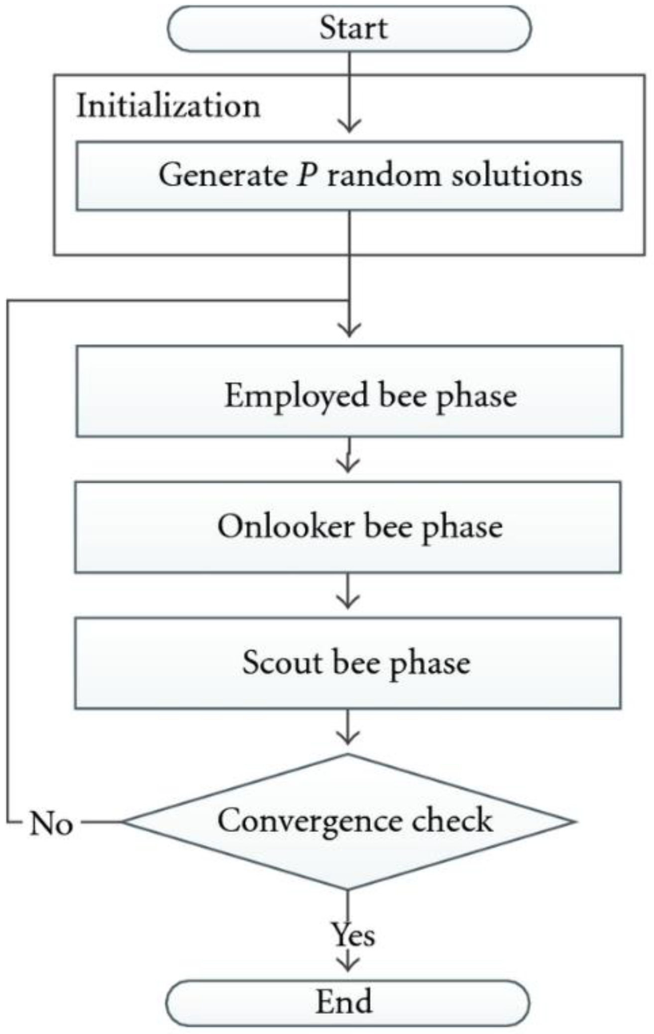
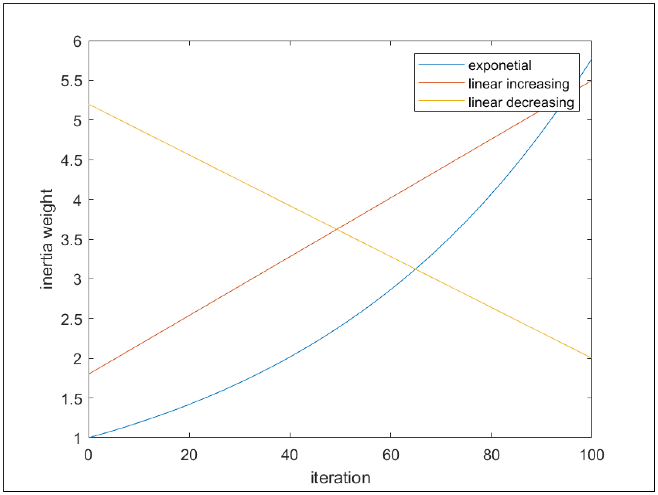
3. Methodology: IW-ABC

The search agents in ABC look for the optimal solution by mimicking the foraging behavior of honeybees. The bees are grouped as employed, onlooker, or scout bees. They work with each other when looking for a food source with abundant nectar. The food source and nectar are analogous to the optimization solution and its fitness or quality. The optimization solution search process can be divided into four phases: initialization, employed bee phase, onlooker bee phase, and scout bee phase. The employed, onlooker, and scout bee phases are iterative processes that are repeated until the stopping condition is satisfied. The stopping condition could either be a maximum number of iterations or the ideal fitness or minimum error. In this research, the maximum number of iterations is adopted as the stopping condition. The general flowchart of the ABC algorithm is shown in Figure 1.

Figure 1. Flowchart of the ABC Algorithm.

3.1. Initialization

The search process starts with an initialization phase where the population’s food sources are randomly generated according to the problem’s search space and dimension, $D$. The population size, $SN$, determines the number of food sources generated and evaluated. An agent ith food source is represented as $x_{ij} where \left(i=1, 2, \dots , SN, j=1,2,\dots , D\right)$.

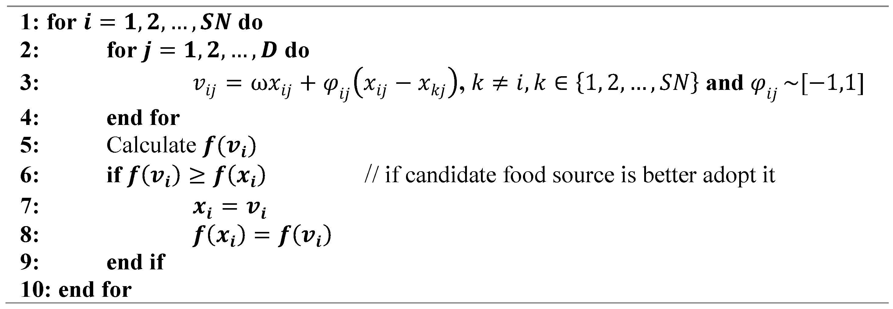
3.2. Employed Bee Phase

The employed bee phase is the first iterative procedure of the ABC where food source information is shared by employed bees in the dance area to the onlooker bees. The onlooker bees then select and remember the food sources according to their nectar amount, $f\left({\mathit{x}}_{\mathit{i}}\right)$, which is the fitness function of the problem to be optimized.

In the IW-ABC, a new candidate food source, $v_{ij}$, is generated using Equation (1).

$$v_{ij}=\omega x_{ij}+{\phi }_{ij}\left(x_{ij}-x_{kj}\right)$$

(1)

where ω is the inertia weight. It controls the influences of the current food source in the generation of the new one. Three type of inertia weight are used here: exponentially increasing inertia weight, linearly increasing inertia weight, and linearly decreasing inertia weight. All of these variants are adaptive according to the iteration number. The exponential inertia weight is shown in Equation (2).

$$\omega =exp \left(\frac{t}{t_{max}}-1\right)$$

(2)

where $t$ is the iteration number, and $t_{max}$ is the maximum iteration number. On the other hand, the linear inertia weight is calculated using Equation (3).

$$\omega =\left(\frac{t_{max}-t}{t_{max}}\right)\left({\omega }_{init}-{\omega }_{final}\right)+{\omega }_{final}$$

(3)

The linear increasing inertia weight is ${\omega }_{init}<{\omega }_{final}$, while the linear decreasing inertia weight is ${\omega }_{init}>{\omega }_{final}$. The rate of the changes for these inertia weights is shown in Figure 2. High inertia encourages exploration and prevents convergence, while small inertia encourages convergence and fine tuning.

Figure 2. Rate of Change of the Inertia Weight.

Based on the second part of Equation (1) it can be seen that the new candidate food source is generated around the current solution, ${\mathit{x}}_{\mathit{i}}$, and a randomly selected solution, ${\mathit{x}}_{\mathit{k}}$, where $k\ne i$ and is randomly selected in the range of $1-SN$. The ${\phi }_{ij}$ is a random number between −1 and 1.

Figure 3 shows the pseudocode for the employed bee phase. For each of the food sources the new candidate food source, ${\mathit{v}}_{\mathit{i}}$, is generated using Equation (1) (line 3 in Figure 3). The fitness of the new candidate food source is then evaluated and if it is better than the current food source, ${\mathit{x}}_{\mathit{i}}$, it is adopted as the food source of the agent.

Figure 3. Pseudo Code of Employed Bee Phase.

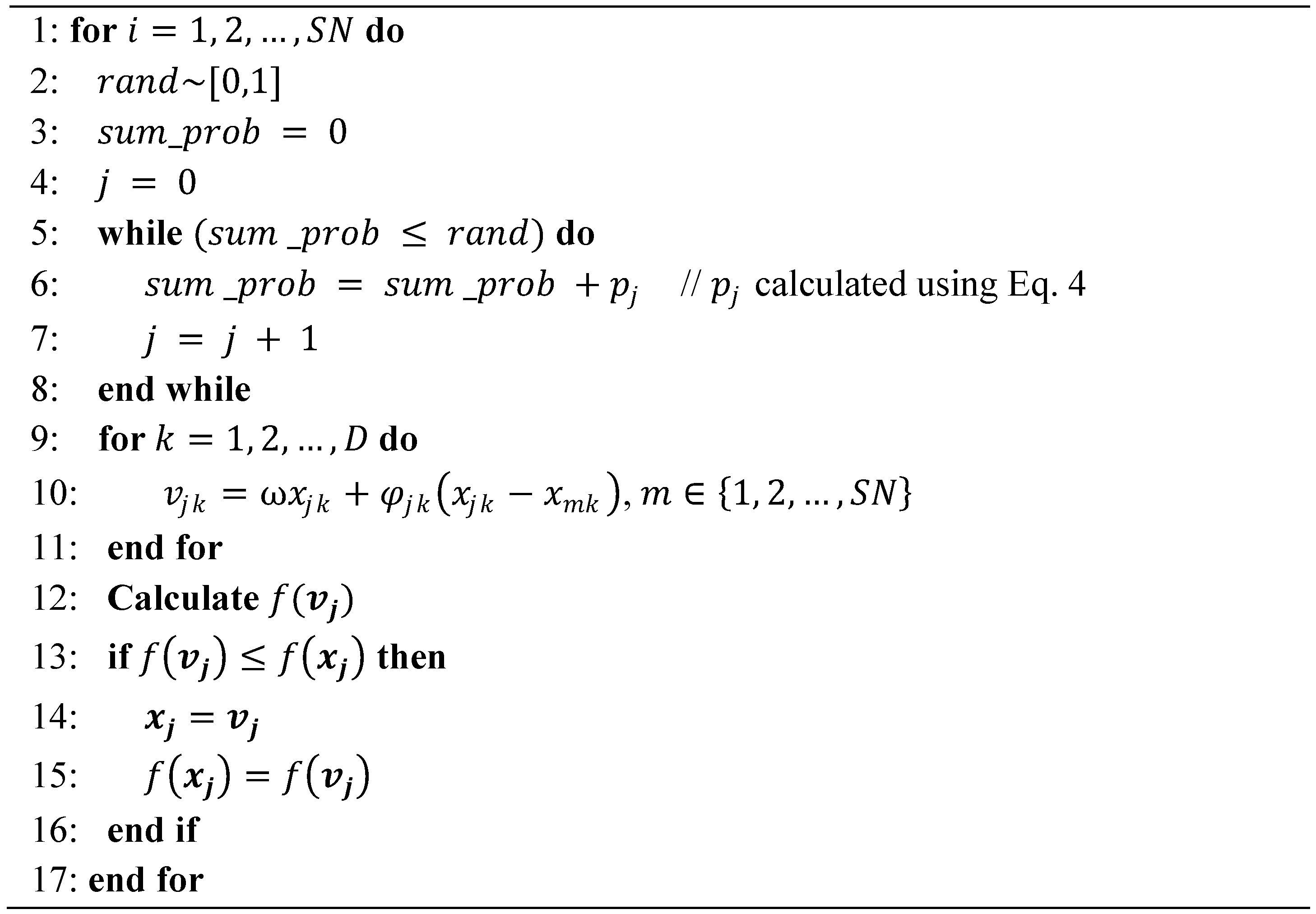
3.3. Onlooker Bee Phase

In the onlooker bee phase a probability value is associated with each food source as given in Equation (4).

$$p_i=\frac{f\left({\mathit{x}}_i\right)}{{{\displaystyle \sum }}_{k=1}^{SN}f\left({\mathit{x}}_k\right)}$$

(4)

Based on this probability value, the onlooker bees determine which of the food sources presented by the onlooker is to be selected.

The pseudocode of the onlooker bee phase is shown in Figure 4. The phase starts with the selection of the random threshold value, $rand$. This value is then compared with the sum of the probability calculated using Equation (4). The food source with a sum probability of more than the random threshold is selected and the candidate food source is calculated using Equation (1). Similar to the employed bee phase, if the new candidate food source is better it is adopted.

Figure 4. Pseudo Code of Onlooker Bee Phase.

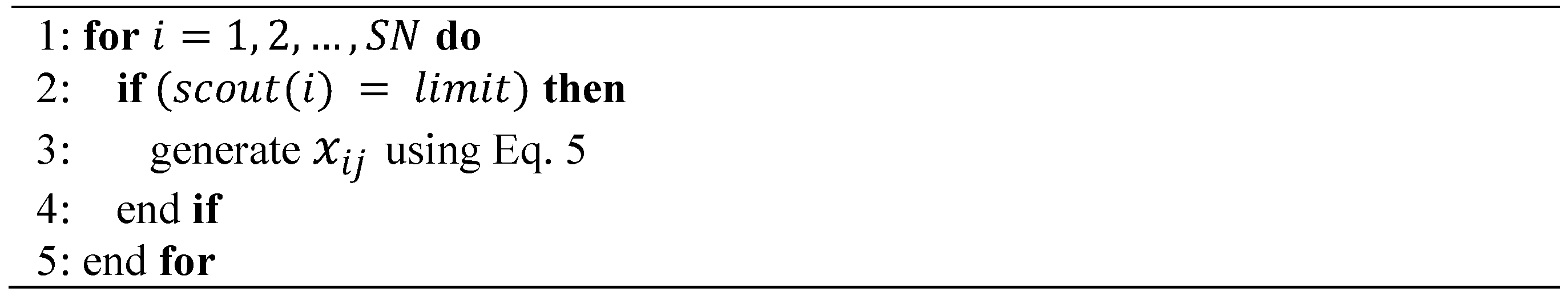
3.4. Scout Bee Phase

A food source is abandoned if no improvement is observed after a number of iterations. These abandoned food sources are then replaced by scout bees who randomly look for new food sources within the search area that is limited by $\left[x_{j\_min},x_{j\_max}\right]$. The random search by scout bees is represented using Equation (5).

$$x_{ij}=x_{j\_min}+rand\left[0,1\right]\left(x_{j\_max}-x_{j\_min}\right)$$

(5)

The pseudocode in Figure 5 is the algorithm of the scout bee phase. The “$limit$” is an important parameter that decides when a food source is abandoned after no improvement for the predetermined number of iterations. The abandoned food source is replaced using Equation (5).

Figure 5. Pseudo Code of Scout Bee Phase.

3.5. Fitness Function

The quality of the solution, $x_i$, is evaluated using the fitness function, $f\left(x_i\right)$, which is defined according to the optimization problem. There are two objectives considered here. The first objective is the occupant’s comfort level maximization, which is measurable using the user comfort index (CI), while the second objective is the minimization of energy consumption of the appliances used to control the room lighting, temperature, and air quality. The fitness function adopted here follows the work of [36].

The comfort index ranges between 0 and 1, where 0 indicates the least comfortable and 1 is when the most comfortable environment is achieved. The comfort index is measured by taking into account the gap between the user’s preference and the room’s environmental values. The lesser the gap the better it is for the occupant. The CI is calculated using Equation (6).

$$CI=p_1 \left[1-{\left(\frac{e_1}{T_s}\right)}^2\right]+p_2 \left[1-{\left(\frac{e_2}{I_s}\right)}^2\right]+p_3 \left[1-{\left(\frac{e_3}{A_s}\right)}^2\right]$$

(6)

where p₁, p₂, and p₃ are the coefficients that control the importance of temperature, illumination, and air quality toward a user’s comfort. These coefficients are defined by the users. The equal values of p₁, p₂, and p₃ indicate the equal importance of all three parameters in providing comfort to the occupant. The errors or differences between the optimized temperature, illumination, and air quality (T_o, I_o, and A_o) and the environmental values (T_c, I_c, and A_c) are represented by e₁, e₂, and e₃, respectively. On the other hand, T_s, I_s, and A_s are the user’s preferred temperature, illumination, and air quality, respectively. The optimized value (T_o, I_o, and A_o) is the evaluated solution i.e., the food source, $x_i$.

The difference between the optimized values and the environment is used for the energy consumption calculation. The amount of energy required by respective appliances is based on this difference. Smaller difference requires smaller energy usage, bigger difference cause higher energy consumption. The total energy consumption is calculated using Equation (7).

$$EC=E_T+E_I+E_A$$

(7)

The energy required by the temperature control actuator is denoted by $E_T$, lighting actuator, $E_I$, and actuator to control the indoor air quality, $E_A.$ Each of these energy requirements can be calculated using Equations (8)–(10), respectively.

$$E_T=P_T\left(T_O-T_C\right)$$

(8)

$$E_I=P_I\left(I_O-I_C\right)$$

(9)

$$E_A=P_A\left(A_O-A_C\right)$$

(10)

where $P_T$ is the energy required per-unit change of the temperature, whereas $P_I$ is the energy required per-unit change of the illumination, and lastly $P_A$ is the energy required per-unit change of the air quality.

The energy saving gain ($G_{es}$) has an inverse relation with the energy consumption. A lower energy consumption leads to higher energy saving gain, where the energy saving gain formula is given in Equation (11).

$$G_{es}=\left(1-{\left(\frac{EC-E_{min}}{E_{max}-E_{min}}\right)}^2\right)$$

(11)

The $E_{min}$ and $E_{max}$ are the minimum and maximum energy and are based on the maximum and minimum of the user preferred temperature, illumination, and air quality.

The two objectives of the user comfort index maximization and energy consumption minimization is tackled as a single objective using the weighted penalty method as shown in Equation (12).

$$Maximize\left(a_1•CI+a_2•G_{ec}\right)$$

(12)

where $a_1$ and $a_2$ determine the importance of CI and $G_{ec}$, respectively, and $a_1+a_2=1$. Equation (12) is the fitness function of the IW-ABC.

4. Experimental Setting

The performance of the IW-ABC is tested using 48 readings of the environmental lighting, temperature, and air quality. The test data are tabulated in Table 2. This dataset is from [33,34], where the data were collected in a laboratory at the Faculty of Computer Science and Information Technology, Universiti Tun Hussein Onn Malaysia for a period of 48 h. The environmental data were periodically recorded on an hourly basis. Many fluctuations in the environmental conditions can be observed during the data collection. The temperature was recorded in the unit of Fahrenheit (°F), illumination in lux, and indoor air quality (IAQ) is in terms of the CO₂ concentration. The preferred setting of the user is as follows: 73 °F, 800 lux, and 800 IAQ. Additionally, the optimized parameters are bounded between 68 and 78 °F, 720 and 880 lux, and 700 and 880 IAQ.

Table 2. Environment’s Temperature, Illumination and Indoor Air Quality.

Time Instances (I)	Temperature (°F)	Illumination (Lux)	Indoor Air Quality (IAQ)
1	60	711	610
2	65	717	670
3	67	718	650
4	66	717	640
5	67	700	600
6	63	713	620
7	62	724	670
8	81	710	920
9	80	914	920
10	81	900	960
11	83	897	900
12	80	895	930
13	79	904	950
14	82	903	960
15	81	906	970
16	80	898	925
17	66	728	610
18	63	703	670
19	66	714	630
20	66	721	645
21	66	722	650
22	67	703	600
23	66	701	670
24	81	728	980
25	81	891	930
26	82	906	948
27	80	901	965
28	81	901	916
29	79	915	900
30	83	914	960
31	79	890	970
32	81	912	930
33	65	717	610
34	67	714	620
35	65	724	670
36	67	726	680
37	66	723	650
38	64	726	660
39	65	708	640
40	80	712	900
41	83	917	910
42	79	905	920
43	82	893	980
44	80	920	940
45	81	913	950
46	81	905	940
47	82	896	970
48	80	898	980

Each of the 48 environmental settings are optimized 30 times. The two objectives of the comfort index maximization and energy consumption minimization have equal importance in this work ($a_1=0.5, a_2=0.5$), this is similar to [36], while the environmental parameters’ influence toward the comfort levels is also set to be equally important ($p_1=\frac{1}{3}, p_2=\frac{1}{3},p_3=\frac{1}{3}$). The energy usage per unit change for temperature, illumination, and air quality ($P_T$, $P_I$ and $P_A$) are also set according to [36]. The range for (${\omega }_{init}, {\omega }_{final}$) of linear increasing and decreasing the IW-ABC is selected based on [26,27]. The parameter setting of the algorithm is shown in Table 3.

Table 3. Algorithms Parameters.

Parameter		Value
Runtime		30
$\mathrm{Maximum} \mathrm{iteration}, t_{max}$		100
Population size		50
Onlooker		Np/2
Limit		(Np/2)*D
Fitness function ratio	$a_1 :a_2$	0.5:0.5
$p_1$		1/3
$p_2$		1/3
$p_3$		1/3
$P_T$		5
$P_I$		1
$P_A$		1
Increasing inertia weight	$[{\omega }_{init} , {\omega }_{final}]$	[0.6, 1.0]
Decreasing inertia weight	$[{\omega }_{init} , {\omega }_{final}]$	[0.9, 0.4]

The comfort index (Equation (6)), energy consumption (Equation (7)), and fitness (Equation (12)) obtained are recorded for a performance measurement. The IW-ABC using exponential, linearly increasing, and linearly decreasing are compared with the original ABC and BA. As discussed before, both ABC and BA had been applied for comfort index maximization and found to outperform other algorithms; hence they are chosen for benchmarking purposes.

The data are then statistically analyzed using non-parametric tests; the Friedman test is used to detect any significant differences, while the Holm post-hoc procedure is used to identify the difference. A significant level of 0.05 or 95% is used here. The Friedman test is a nonparametric statistical analysis that is frequently used for the comparison of three or more metaheuristic algorithms [50,51]. While the Holm post-hoc test is usually paired with the Friedman test to find the algorithms that are on par or are significantly worse than the best algorithm. In this work, the statistical analysis is done using KEEL, an open source software developed to assess algorithm performance [52,53,54].

5. Results and Discussion

The algorithms’ average, maximum, and minimum of fitness, comfort index, and energy consumption from the 30 runs are tabulated together with the Friedman rank and the Holm post hoc procedure p-values in Table 4. The best of the average, maximum, minimum, and Friedman rank are highlighted in grey, while the Holm’s p-values that indicate significant differences are in bold.

Table 4. Algorithms Performance.

		Average	Max	Min	Friedman Rank	Holm Post Hoc
Fitness	ABC	0.9799	0.9975	0.9633	4.1771	0 < 0.0125
	IW-ABC (exponential)	0.9853	0.9999	0.9596	2.9687	0.04898 > 0.016667
	IW-ABC (linear increasing)	0.9863	0.9999	0.9608	2.6667	0.3017 > 0.05
	IW-ABC (linear decreasing)	0.9869	0.9999	0.9722	2.3333
	BA	0.9838	0.9977	0.9684	2.8542	0.106583 > 0.025
Comfort Index	ABC	0.9913	0.9966	0.9821	5.9583	0 < 0.01
	IW-ABC (exponential)	0.9960	0.9997	0.9883	2.5521	0.518387 > 0.025
	IW-ABC (linear increasing)	0.9963	0.9997	0.9917	2.2292
	IW-ABC (linear decreasing)	0.9962	0.9997	0.9910	2.2396	0.983379 > 0.05
	FA	0.9915	0.9961	0.9752	5.7083	0 < 0.0125
	ACO	0.9909	0.9975	0.9796	6.5000	0 < 0.008333
	GA	0.9901	0.9978	0.9793	6.8542	0 < 0.007143
	BA	0.9945	0.9994	0.9839	3.9583	0.000544 < 0.016667
Energy Consumption	ABC	147.6226	214.8538	68.1349	4.1458	0 < 0.0125
	IW-ABC (exponential)	120.9565	222.4773	31.0000	2.8229	0.258636 > 0.025
	IW-ABC (linear increasing)	116.1257	202.4568	31.0000	2.5312	0.821261 > 0.05
	IW-ABC (linear decreasing)	117.0123	214.2358	27.6068	2.4583
	BA	131.1864	216.9695	68.0068	3.0417	0.070701 > 0.016667

The results of the fitness optimization, which combines both the comfort index maximization and energy consumption minimization, show that the IW-ABC with linearly decreasing inertia in the range between 0.9 and 0.4 is better than the others. The Friedman rank of this variant of IW-ABC is the best at 2.3333, while the Friedman statistic value is 37.695833. This shows significant differences exist between the algorithms. The Holm post hoc test shows that the linearly decreasing IW-ABC is significantly better than the original ABC, but is on par with BA. All variants of the IW-ABC investigated here show on-par performance.

The effect of the optimization algorithms toward each of the objectives is then studied using the optimized parameters. The dataset comes with results from the comfort index maximization using FA, ACO, GA, and BA, where the results are optimized without taking the energy consumption into consideration. Hence, for fairness, only the comfort index is statistically analyzed against these algorithms. The IW-ABC with linearly increasing inertia weight from 0.6 to 1 reported the best comfort index optimization performance. The comfort index found by the linearly increasing IW-ABC has the best Friedman rank followed by linear decreasing and exponential inertia weight. The comfort index found by BA and FA are better than the original ABC. However, the original ABC is better than ACO and GA in optimizing the comfort index. The Friedman statistic of 219.862847 showed a significant difference between the algorithms. The p-values of the Holm post hoc test indicate that the linearly increasing IW-ABC is significantly better than the original ABC, FA, ACO, GA, and BA, and has an on-par performance with the other two variants of the IW-ABC investigated here.

In terms of the energy consumption minimization, the linear decreasing IW-ABC has the best Friedman rank. The Friedman statistic is 35.695833, rejecting the null hypothesis of on-par performance for all algorithms tested. The Holm post hoc p-values indicate the linear decreasing IW-ABC is significantly better than the original ABC but not significantly better than the BA. All the variants of the IW-ABC have on-par performance.

The fitness of the optimization algorithms over the 48 time instances are illustrated in Figure 6. The optimization algorithms are able to improve the fitness value. As shown in the graph, after optimization using exponential the IW-ABC (green), linear increasing IW-ABC (orange), linear decreasing IW-ABC (purple), ABC (red), and BA (sky-blue), all the fitness values are above the dark blue line, which is the fitness value before optimization. The IW-ABC with linearly decreasing inertia weight provides the highest fitness value in comparison to the other algorithms in most of the time instances as can be seen from the purple line in the figure.

Figure 6. Fitness vs. Time Instance.

The user comfort index of the optimization process is shown in Figure 7. The optimized comfort index values regardless of the optimizer used are constantly better than the comfort index value of the non-optimized system shown by the dark blue line. This shows the optimization algorithms are able to optimize the user comfort index. However, among all the algorithms, the three variants of IW-ABC (exponential in orange, linear decreasing in green, and linear increasing in purple) show better performance where the lines are closer to 1. The BA (apricot) and FA (sky-blue) are close to the proposed variants of IW-ABC. Meanwhile, the ABC (red), ACO (maroon), and GA (blue) perform worse but are, nonetheless, better than without optimization. The fluctuation of the comfort index is influenced by the fluctuation in the environment.

Figure 7. Comfort Index vs. Time Instance.

The total power consumption of the optimization process can be seen in Figure 8. Similar to the fitness and comfort index, the energy consumption using the optimized parameters is better than the non-optimized system in the dark blue line. The optimization algorithms successfully reduce the energy usages. The exponential IW-ABC (green), linear increasing IW-ABC (orange), and linear decreasing IW-ABC (purple) are lower than ABC (red) and BA (sky-blue) for most of the time instance.

Figure 8. Energy Consumption vs. Time Instance.

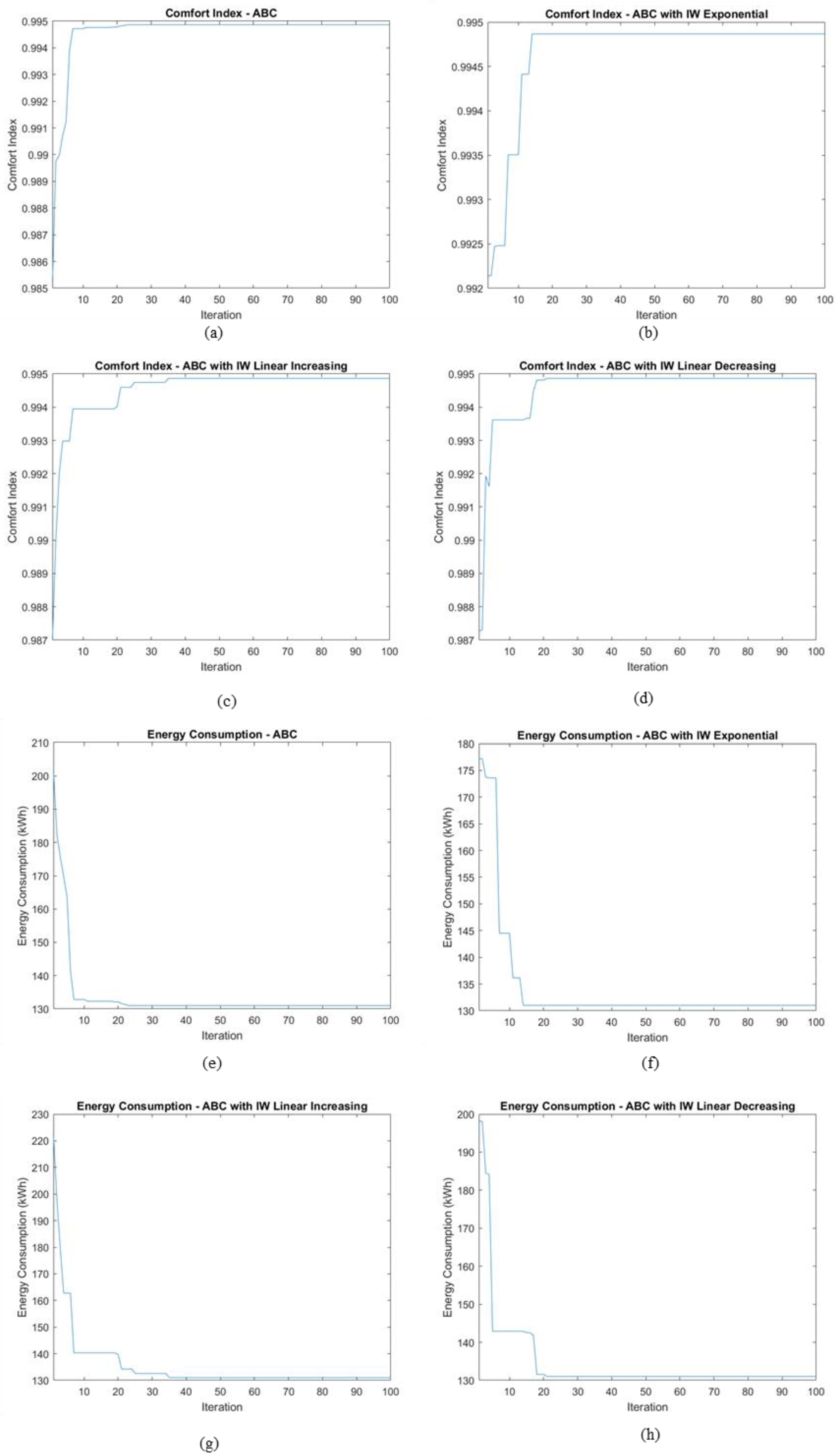
5.1. Convergence Analysis

The inertia weight is frequently introduced to improve the exploration and exploitation of metaheuristic algorithms. This is the motivation for the application of the IW-ABC here. The contribution of inertia weight can be observed using the convergence curve for a selected time instance.

The convergence of the comfort index and energy consumption of the IW-ABC with exponential, linear increasing, and linear decreasing are compared with the original ABC in Figure 9. It could be observed (Figure 9a,e) that the original ABC suffers from fast convergence and imbalanced exploration and exploitation. The original ABC started to converge even before the 10 th iteration.

Figure 9. Convergence Curves of Comfort Index and Energy Consumption.

The convergence of the linear increasing IW-ABC (Figure 9c,g) is delayed the most followed by linear decreasing (Figure 9b,f) and exponential (Figure 9d,h). This is desired as it balances between exploration during the first half of the iteration and exploitation in the later half.

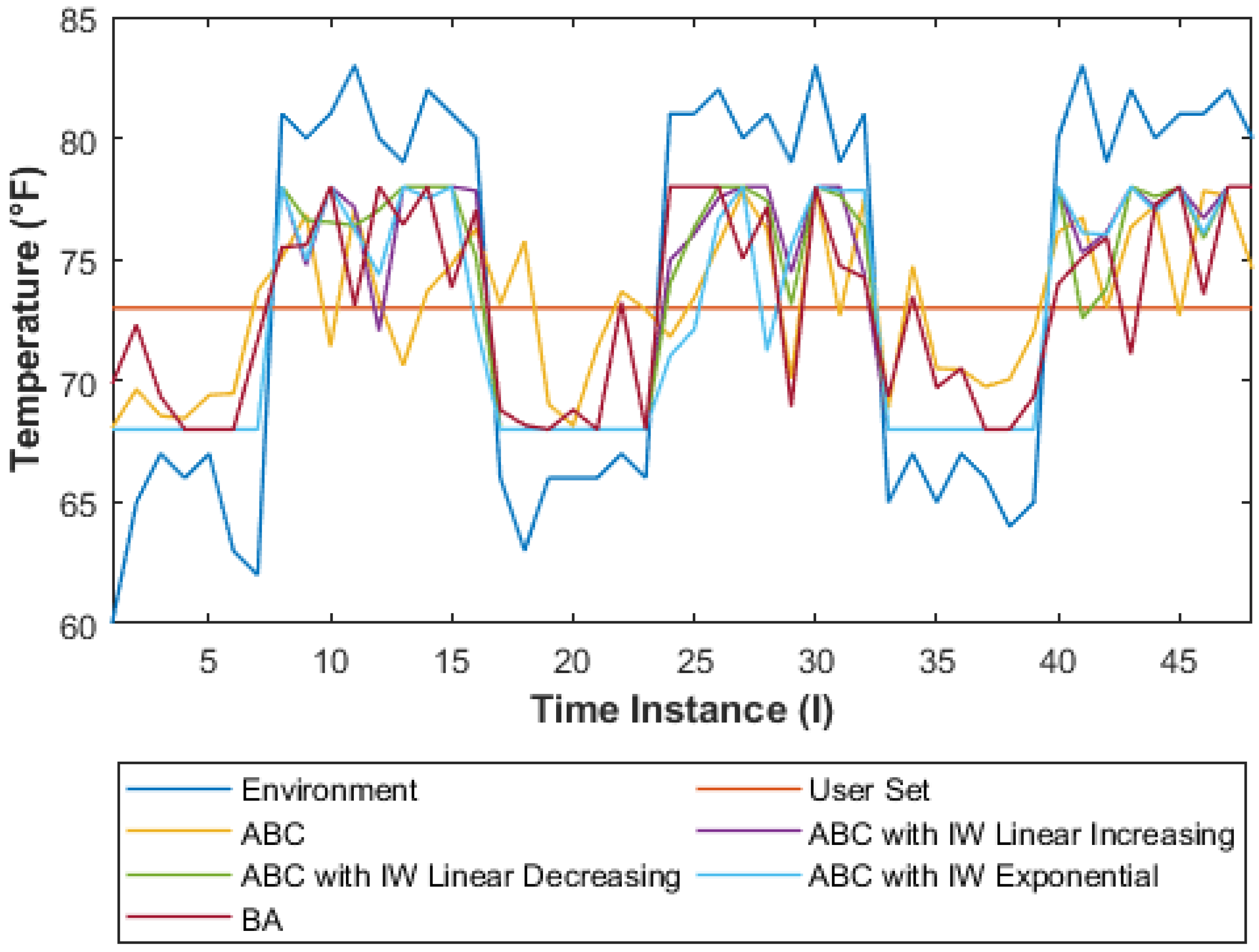
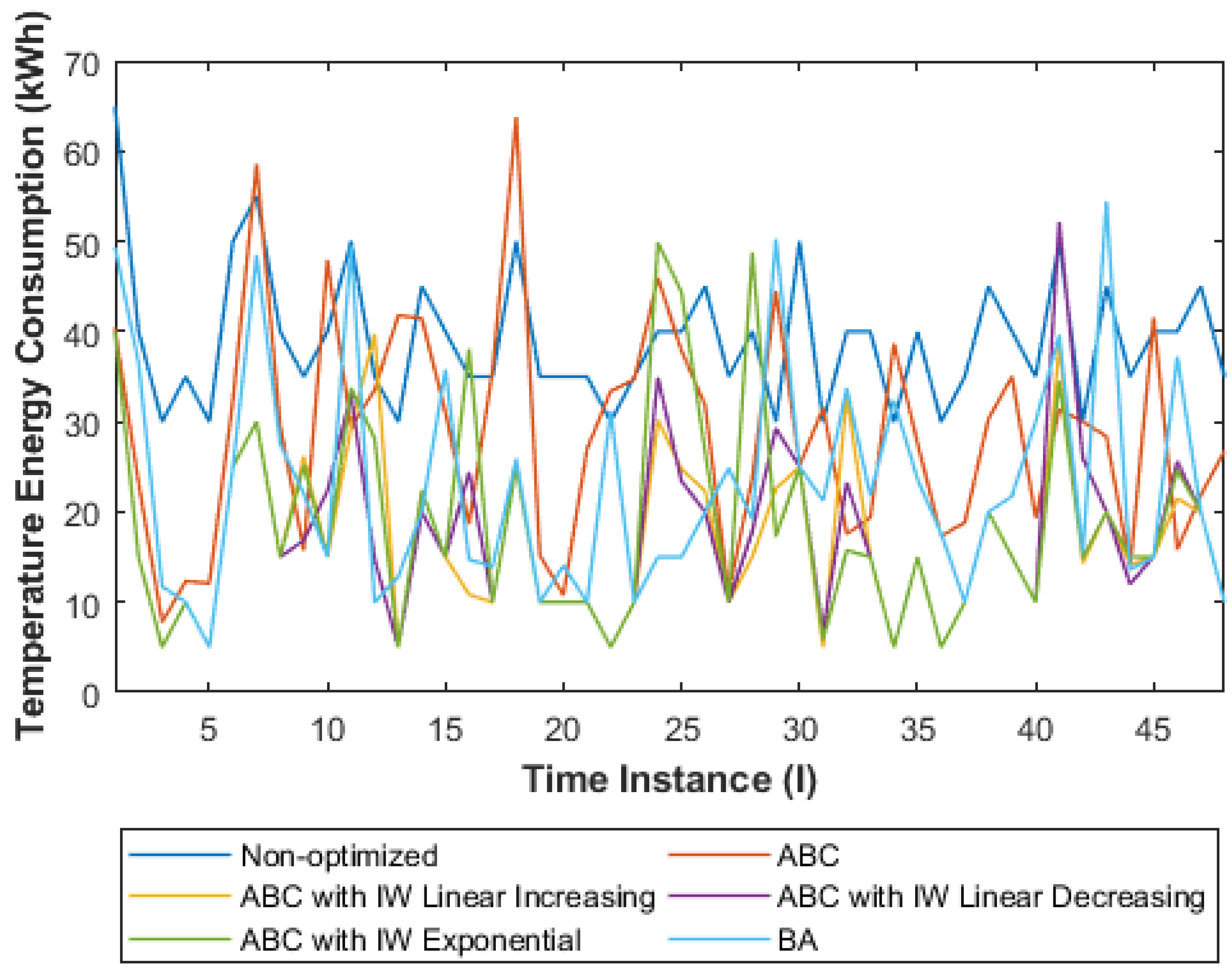
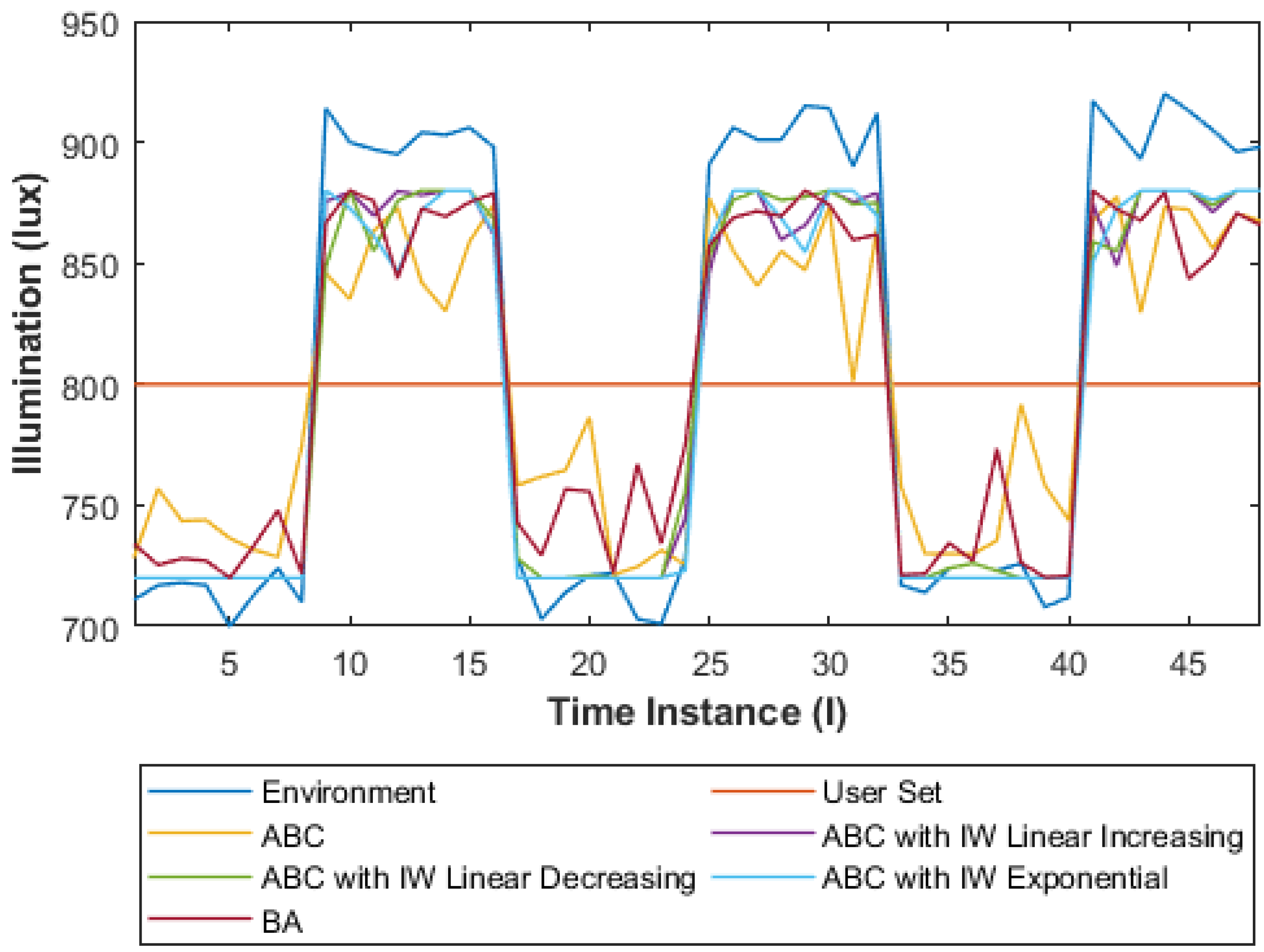
5.2. Optimized Parameters

Figure 10 shows the environmental temperature, user set temperature, and the optimized temperatures according to the algorithms. The optimized values oscillate within the bounded limit of [68 °F, 78 °F] and all are in between the environmental temperature value (dark blue) and approaching the user set value (red). The oscillation is influenced by the change of the environmental temperature. The optimizers aim to minimize the error difference between the optimized temperature and user’s preference so that the comfort index is maximized, while at the same time reducing the difference of the optimized temperature with the environment so that the energy usage is reduced. The energy consumption in optimizing the temperature is shown in Figure 11. The energy required for the system using optimized temperatures are lower than the non-optimized system in most of the settings. The exponential IW-ABC (in green) is observed to contribute to lower energy usage.

Figure 10. Optimized Temperature vs. Time Instance.

Figure 11. Energy Consumption for Temperature Optimization.

For the illumination parameter optimization, the results are shown in Figure 12. Similar to the temperature, as the optimizers balanced between the comfort index maximization and power consumption minimization, the optimized illumination values obtained are between the environmental value and the user’s demand. The optimized illumination was also in the predefined limit. Figure 13 shows the required energy of illumination. The optimized energy consumption is lower than the non-optimized system for all time instances. Thus, the required energy consumption of the lighting system is successfully reduced using the optimization system. The IW-ABC with linear decreasing inertia weight (in purple) found the best illumination level with the lowest energy usage.

Figure 12. Optimized Illumination vs. Time Instance.

Figure 13. Energy Consumption for Illumination Optimization.

The optimized air quality with respect to the environmental and user preferred air quality are shown in Figure 14. The optimized air quality values are in between the environmental value, the user set value, and the limit of 700, 880 IAQ. The optimized air quality compromises between the comfort index and energy consumption. Figure 15 shows the required energy for air quality optimization. The ventilation system requires lesser energy after optimization. Moreover, the three variants of IW-ABC offer better energy efficiency than ABC and BA.

Figure 14. Optimized Air Quality vs. Time Instance.

Figure 15. Power Consumption for Air Quality Optimization.

6. Conclusions

This project aimed to optimize the residential user comfort index and energy consumption using an improved version of the ABC algorithm. The ABC is improved using inertia weight, IW-ABC. Inertia weight is popularly adopted in many metaheuristic algorithms for a convergence improvement, so that the exploration and exploitation can be better controlled and premature convergence can be avoided. The findings show that the IW-ABC improves the ABC and performs better than the BA. In terms of comfort index maximization, the IW-ABC is better than the original ABC, FA, ACO, GA, and BA. The linear increasing inertia has the most improved convergence rate where the algorithm only converges after 40% of the total iteration. The variant of IW-ABC also has the best comfort index of 0.9997. This research is conducted using secondary data from [33,34]. In the future, the proposed optimization system is to be implemented and integrated in smart home controllers where the IW-ABC acts as the brain and searches for optimized parameter values for the actuators’ input.

References

1. Klepeis, N.E.; Nelson, W.C.; Ott, W.R.; Robinson, J.P.; Tsang, A.M.; Switzer, P.; Behar, J.V.; Hern, S.C.; Engelmann, W.H. The National Human Activity Pattern Survey (NHAPS): A resource for assessing exposure to environmental pollutants. J. Expo. Anal. Environ. Epidemiol. 2001, 11, 231–252. [Google Scholar] [CrossRef] [PubMed]
2. Khajehzadeh, I.; Vale, B. How New Zealanders distribute their daily time between home indoors, home outdoors and out of home. Kōtuitui N. Z. J. Soc. Sci. Online 2017, 12, 17–23. [Google Scholar] [CrossRef]
3. Banerjee, D.; Rai, M. Social isolation in COVID-19: The impact of loneliness. Int. J. Soc. Psychiatry 2020, 66, 525–527. [Google Scholar] [CrossRef] [PubMed]
4. Flanagan, E.W.; Beyl, R.A.; Fearnbach, S.N.; Altazan, A.D.; Martin, C.K.; Redman, L.M. The Impact of COVID-19 Stay-At-Home Orders on Health Behaviors in Adults. Obesity 2021, 29, 438–445. [Google Scholar] [CrossRef] [PubMed]
5. Lund, S.; Madgavkar, A.; Manyika, J.; Smit, S.; Ellingrud, K.; Meaney, M.; Robinson, O. The future of work after COVID-19. McKinsey Glob. Inst. 2021, 18, 152. [Google Scholar]
6. Chung, H.; Seo, H.; Forbes, S.; Birkett, H. Working from Home during the COVID-19 Lockdown: Changing Preferences and the Future of Work. 2020. Available online: https://kar.kent.ac.uk/83896/ (accessed on 1 May 2022).
7. Hu, M.; Simon, M.; Fix, S.; Vivino, A.A.; Bernat, E. Exploring a sustainable building’s impact on occupant mental health and cognitive function in a virtual environment. Sci. Rep. 2021, 11, 5644. [Google Scholar] [CrossRef]
8. Tham, S.; Thompson, R.; Landeg, O.; Murray, K.A.; Waite, T. Indoor temperature and health: A global systematic review. Public Health 2020, 179, 9–17. [Google Scholar] [CrossRef]
9. Kamaruzzaman, S.N.; Sabrani, N.A. The effect of Indoor Air Quality (IAQ) towards occupants’ psychological performance in office buildings. J. Rekabentuk Dan Binaan 2011, 4, 49–61. [Google Scholar]
10. Osibona, O.; Solomon, B.D.; Fecht, D. Lighting in the home and health: A systematic review. Int. J. Environ. Res. Public Health 2021, 18, 609. [Google Scholar] [CrossRef]
11. Grimaldi, S.; Partonen, T.; Saarni, S.I.; Aromaa, A.; Lönnqvist, J. Indoors illumination and seasonal changes in mood and behavior are associated with the health-related quality of life. Health Qual. Life Outcomes 2008, 6, 56. [Google Scholar] [CrossRef]
12. Yang, X.S. Review of Metaheuristics and Generalized Evolutionary Walk Algorithm. arXiv 2011, arXiv:1105.3668. [Google Scholar]
13. Kennedy, J.; Eberhart, R. Particle swarm optimization. In Proceedings of the IEEE International Conference on Neural Networks, IEEE, Perth, Australia, 27 November–1 December 1995; Volume 4, pp. 1942–1948. [Google Scholar]
14. Karaboga, D. An Idea Based on Honey Bee Swarm for Numerical Optimization. Tech. Rep. Tr06 Erciyes Univ. Eng. Fac. Comput. Eng. Dep. 2005. Available online: https://abc.erciyes.edu.tr/pub/tr06_2005.pdf (accessed on 1 May 2022).
15. Yang, X.S. A new metaheuristic Bat-inspired Algorithm. In Studies in Computational Intelligence; González, J.R., Ed.; Springer: Berlin/Heidelberg, Germany, 2010; pp. 65–74. [Google Scholar]
16. Yang, X.S. Nature-Inspired Metaheuristic Algorithms; Luniver Press: Rome, Italy, 2008. [Google Scholar]
17. Holland, J.H. Adaptation in Natural and Artificial Systems: An Introductory Analysis with Applications to Biology, Control and Artificial Intelligence; MIT Press: Cambridge, MA, USA, 1992. [Google Scholar]
18. Karaboga, D.; Akay, B. A comparative study of Artificial Bee Colony algorithm. Appl. Math. Comput. 2009, 214, 108–132. [Google Scholar] [CrossRef]
19. Sharma, A.; Sharma, A.; Choudhary, S.; Pachauri, R.K.; Shrivastava, A.; Kumar, D. A Review on Artificial Bee Colony and Its Engineering Applications. J. Crit. Rev. 2020, 7, 4097–4107. [Google Scholar]
20. Vargas Benítez, C.M.; Lopes, H.S. Parallel artificial bee colony algorithm approaches for protein structure prediction using the 3DHP-SC model. Stud. Comput. Intell. 2010, 315, 255–264. [Google Scholar]
21. Ma, M.; Liang, J.; Guo, M.; Fan, Y.; Yin, Y. SAR image segmentation based on artificial bee colony algorithm. Appl. Soft Comput. J. 2011, 11, 5205–5214. [Google Scholar] [CrossRef]
22. Cao, M.L.; Hu, X. Robust pollution source parameter identification based on the artificial bee colony algorithm using a wireless sensor network. PLoS ONE 2020, 15, e0232843. [Google Scholar] [CrossRef]
23. Zhang, T.; Chen, G.; Zeng, Q.; Song, G.; Li, C.; Duan, H. Seamless clustering multi-hop routing protocol based on improved artificial bee colony algorithm. Eurasip J. Wirel. Commun. Netw. 2020, 2020, 75. [Google Scholar] [CrossRef]
24. Sonmez, M. Artificial Bee Colony algorithm for optimization of truss structures. Appl. Soft Comput. J. 2011, 11, 2406–2418. [Google Scholar] [CrossRef]
25. Shi, Y.; Eberhart, R.C. Empirical study of particle swarm optimization. In Proceedings of the 1999 Congress on Evolutionary Computation-CEC99 (Cat. No. 99TH8406), Washington, DC, USA, 6–9 July 1999; pp. 1945–1950. [Google Scholar]
26. Elkhateeb, N.A.; Badr, R.I. Employing Artificial Bee Colony with dynamic inertia weight for optimal tuning of PID controller. In Proceedings of the 2013 5th International Conference on Modelling, Identification and Control (ICMIC), Cairo, Egypt, 31 August–2 September 2013; Volume 2013, pp. 42–46. [Google Scholar]
27. Nie, L.; Mao, M.; Wan, Y.; Cui, L.; Zhou, L.; Zhang, Q. Maximum power point tracking control based on modified abc algorithm for shaded PV system. In Proceedings of the 2019 AEIT International Conference of Electrical and Electronic Technologies for Automotive (Aeit Automotive), Turin, Italy, 2–4 July 2019. [Google Scholar]
28. Jia, L.; Wei, S.; Liu, J. A review of optimization approaches for controlling water-cooled central cooling systems. Build. Environ. 2021, 203, 108100. [Google Scholar] [CrossRef]
29. Shah, A.S.; Nasir, H.; Fayaz, M.; Lajis, A.; Shah, A. A review on energy consumption optimization techniques in IoT based smart building environments. Information 2019, 10, 108. [Google Scholar] [CrossRef]
30. Ali, S.; Kim, D.H. Optimized Power Control Methodology Using Genetic Algorithm. Wirel. Pers. Commun. 2015, 83, 493–505. [Google Scholar] [CrossRef]
31. Wahid, F.; Kim, D.H. An Efficient Approach for Energy Consumption Optimization and Management in Residential Building Using Artificial Bee Colony and Fuzzy Logic. Math. Probl. Eng. 2016, 2016, 9104735. [Google Scholar] [CrossRef]
32. Wahid, F.; Ghazali, R.; Ismail, L.H. An Enhanced Approach of Artificial Bee Colony for Energy Management in Energy Efficient Residential Building. Wirel. Pers. Commun. 2019, 104, 235–257. [Google Scholar] [CrossRef]
33. Wahid, F.; Ismail, L.H.; Ghazali, R.; Aamir, M. An efficient artificial intelligence hybrid approach for energy management in intelligent buildings. KSII Trans. Internet Inf. Syst. 2019, 13, 5904–5927. [Google Scholar]
34. Wahid, F.; Ghazali, R.; Ismail, L.H. Improved Firefly Algorithm Based on Genetic Algorithm Operators for Energy Efficiency in Smart Buildings. Arab. J. Sci. Eng. 2019, 44, 4027–4047. [Google Scholar] [CrossRef]
35. Shah, A.S.; Nasir, H.; Fayaz, M.; Lajis, A.; Ullah, I.; Shah, A. Dynamic User Preference Parameters Selection and Energy Consumption Optimization for Smart Homes Using Deep Extreme Learning Machine and Bat Algorithm. IEEE Access 2020, 8, 204744–204762. [Google Scholar] [CrossRef]
36. Ullah, I.; Kim, D. An improved optimization function for maximizing user comfort with minimum energy consumption in smart homes. Energies 2017, 10, 1818. [Google Scholar] [CrossRef]
37. Li, J.; Yin, S.W.; Shi, G.S.; Wang, L. Optimization of indoor thermal comfort parameters with the adaptive network-based fuzzy inference system and particle swarm optimization algorithm. Math. Probl. Eng. 2017, 2017, 3075432. [Google Scholar] [CrossRef]
38. Taylor, M.; Brown, N.C.; Rim, D. Optimizing thermal comfort and energy use for learning environments. Energy Build. 2021, 248, 111181. [Google Scholar] [CrossRef]
39. Khan, Z.A.; Zafar, A.; Javaid, S.; Aslam, S.; Rahim, M.H.; Javaid, N. Hybrid meta-heuristic optimization based home energy management system in smart grid. J. Ambient Intell. Humaniz. Comput. 2019, 10, 4837–4853. [Google Scholar] [CrossRef]
40. Khalid, A.; Zafar, A.; Abid, S.; Khalid, R.; Khan, Z.A.; Qasim, U.; Javaid, N. Cuckoo search optimization technique for multi-objective home energy management. Adv. Intell. Syst. Comput. 2017, 612, 520–529. [Google Scholar]
41. Wahid, F.; Ghazali, R.; Fayaz, M.; Shah, A.S.; Tun, U.; Onn, H. A Simple and Easy Approach for Home Appliances Energy Consumption Prediction in Residential Buildings Using Machine Learning Techniques. J. Appl. Environ. Biol. Sci. 2017, 7, 108–119. [Google Scholar]
42. Wahid, F.; Kim, D.H. A prediction approach for demand analysis of energy consumption using K-nearest neighbor in residential buildings. Int. J. Smart Home 2016, 10, 97–108. [Google Scholar] [CrossRef]
43. Wahid, F.; Ghazali, R.; Shah, A.S.; Fayaz, M. Prediction of Energy Consumption in the Buildings Using Multi-Layer Perceptron and Random Forest. Int. J. Adv. Sci. Technol. 2017, 101, 13–22. [Google Scholar] [CrossRef]
44. Wahid, F.; Kim, D.H. Short-term energy consumption prediction in Korean residential buildings using optimized multi-layer perceptron. Kuwait J. Sci. 2017, 44, 67–77. [Google Scholar]
45. Khan, Z.A.; Ullah, A.; Ullah, W.; Rho, S.; Lee, M.; Baik, S.W. Electrical energy prediction in residential buildings for short-term horizons using hybrid deep learning strategy. Appl. Sci. 2020, 10, 8624. [Google Scholar] [CrossRef]
46. Bot, K.; Ruano, A.; da Graça Ruano, M. Forecasting Electricity Consumption in Residential Buildings for Home Energy Management Systems. Commun. Comput. Inf. Sci. 2020, 1237, 313–326. [Google Scholar]
47. Zhang, Y.; Chen, Q. Prediction of building energy consumption based on PSO—RBF neural network. In Proceedings of the 2014 IEEE International Conference on System Science and Engineering, Shanghai, China, 11–13 July 2014; pp. 60–63. [Google Scholar]
48. Chegari, B.; Tabaa, M.; Simeu, E.; Moutaouakkil, F.; Medromi, H. Multi-objective optimization of building energy performance and indoor thermal comfort by combining artificial neural networks and metaheuristic algorithms. Energy Build. 2021, 239, 110839. [Google Scholar] [CrossRef]
49. Liu, W.; Sui, P.; Wang, C. Improved Particle Swarm Optimization Algorithm Based on Social Psychology. In Proceedings of the International Conference on Artificial Intelligence and Computational Intelligence, Shanghai, China, 7–8 November 2009; pp. 145–148. [Google Scholar]
50. Derrac, J.; García, S.; Molina, D.; Herrera, F. A practical tutorial on the use of nonparametric statistical tests as a methodology for comparing evolutionary and swarm intelligence algorithms. Swarm Evol. Comput. 2011, 1, 3–18. [Google Scholar] [CrossRef]
51. García, S.; Molina, D.; Lozano, M.; Herrera, F. A Study on The Use of Non-parametric Tests for Analyzing The Evolutionary Algorithms’ Behaviour: A Case Study on The CEC’2005 Special Session on Real Parameter Optimization. J. Heuristics 2008, 15, 617–644. [Google Scholar] [CrossRef]
52. Alcalá-Fdez, J.; Fernández, A.; Luengo, J.; Derrac, J.; García, S.; Sánchez, L.; Herrera, F. KEEL data-mining software tool: Data set repository, integration of algorithms and experimental analysis framework. J. Mult. Log. Soft Comput. 2011, 17, 255–287. [Google Scholar]
53. Triguero, I.; González, S.; Moyano, J.M.; García, S.; Alcalá-Fdez, J.; Luengo, J.; Fernández, A.; del Jesús, M.J.; Sánchez, L.; Herrera, F. KEEL 3.0: An Open Source Software for Multi-Stage Analysis in Data Mining. Int. J. Comput. Intell. Syst. 2017, 10, 1238. [Google Scholar] [CrossRef]
54. Alcalá-Fdez, J.; Sánchez, L.; García, S.; del Jesus, M.J.; Ventura, S.; Garrell, J.M.; Otero, J.; Romero, C.; Bacardit, J.; Rivas, V.M.; et al. KEEL: A software tool to assess evolutionary algorithms for data mining problems. Soft Comput. 2009, 13, 307–318. [Google Scholar] [CrossRef]
Publisher’s Note: MDPI stays neutral with regard to jurisdictional claims in published maps and institutional affiliations.
Article Metrics
Citations
Article Access Statistics
Multiple requests from the same IP address are counted as one view.