Computational Performance Evaluation of Column Generation and Generate-and-Solve Techniques for the One-Dimensional Cutting Stock Problem

Abstract

The Cutting Stock Problem (CSP) is an optimisation problem that roughly consists of cutting large objects in order to produce small items. The computational effort for solving this problem is largely affected by the number of cutting patterns. In this article, in order to cope with large instances of the One-Dimensional Cutting Stock Problem (1D-CSP), we resort to a pattern generating procedure and propose a strategy to restrict the number of patterns generated. Integer Linear Programming (ILP) models, an implementation of the Column Generation (CG) technique, and an application of the Generate-and-Solve (G&S) framework were used to obtain solutions for benchmark instances from the literature. The exact method was capable of solving small and medium sized instances of the problem. For large sized instances, the exact method was not applicable, while the effectiveness of the other methods depended on the characteristics of the instances. In general, the G&S method presented successful results, obtaining quasi-optimal solutions for the majority of the instances, by employing the strategy of artificially reducing the number of cutting patterns and by exploiting them in a heuristic framework.

1. Introduction

The CSP is an optimisation problem that basically consists of cutting larger parts (objects) available in stock in order to produce smaller parts (items) to meet a given demand, optimising a certain objective function, for example, the loss of material or the cost of the objects to be cut. This problem belongs to the NP-Hard class [1], that is, there is no deterministic algorithm that can solve it in polynomial time with certificate of optimality, unless P = NP. Thus, for large sized instances of the problem to be tackled efficiently, it is necessary to resort to approximation algorithms, such as heuristics and metaheuristics, and, therefore, the guarantee of optimality is lost in order to obtain good solutions in a reasonable time.

Applications of this problem are commonly found in a wide variety of industries in which the waste of materials is a major concern, such as in manufacturing processes of steel, textile, paper, and glass. It is important to note that, in real world applications, different constraints may be considered due to the particularities of the manufacturing processes involved in each scenario. Given its wide applicability, in addition to its theoretical relevance, the search for increasingly promising solutions to this problem is still very relevant [2].

In this work, we propose a procedure for generating cutting patterns for the 1D-CSP and a strategy for reducing the number of patterns generated, in order to deal with large scale instances of the problem, even if the guarantee of obtaining an optimal solution is lost. Using benchmark instances from the literature [3], computational experiments were performed for two ILP models, an implementation of the classical CG technique [4,5,6], and an application of the G&S framework [7,8,9,10].

We employed CPLEX [11] for solving the ILP models. We resorted to Coluna [12] for running the CG technique and Java Concert for implementing the G&S method to tackle the problem. The exact method was able to solve only small and medium sized instances. None of the CG and G&S algorithms stood out from the other for all instances. In fact, the effectiveness varied according to the characteristics of the instances, such as the number of item types, the size of the items in relation to the size of the object, and the demand for each item type. Roughly, G&S performed well for all classes, obtaining quasi-optimal solutions for the majority of the instances.

The remainder of this article is structured as it follows: in Section 2, we formally state the 1D-CSP, discuss the approaches commonly used to solve it, and introduce the G&S framework. In Section 3, we present a procedure for generating cutting patterns for the 1D-CSP and propose a strategy for artificially reducing the number of patterns to be considered into the formulation. In addition, we explain in detail the application of this methodology to the 1D-CSP. Section 4 is dedicated to present and analyse the computational results obtained from the different approaches. In Section 5, final remarks and perspectives on future work conclude the article.

2. Preliminaries

In this section, we formally introduce the 1D-CSP, review the literature on the CG technique, and present the G&S methodology.

2.1. The Cutting Stock Problem

The CSP was first described by Kantorovich in 1939 and later published in [13]. This problem presents many variations, but it can be usually classified according to its dimensional aspect: one-dimensional (1D), two-dimensional (2D), and three-dimensional (3D)—and as to the length of stock objects—single or multiple. In this article, according to the classification proposed by Wäscher et al. in [14], the variant known in the literature as One-Dimensional Simple Stock Size Cutting Stock Problem is considered, characterised by one-dimensional cutting patterns obtained from large identical objects of fixed dimension, and it can be seen as a generalisation of the Bin Packing Problem (BPP) [15].

The 1D-CSP can be formally stated as follows. Consider large objects of length L in stock and a set of m different types of items characterised by a length $l_i\le L$ and a demand $d_i\in {\mathbb{Z}}^{+}$, $i=1,2,\cdots ,m$. A cutting pattern describes how many items of each type are cut from a stock object, and it can be represented by a vector $a_j={(a_{1j},a_{2j},\cdots ,a_{mj})}^T$, where $a_{ij}$ indicates the quantity of items of the type i obtained by cutting an object according to the cutting pattern $a_j(j=1,2,\cdots ,n)$. For the cutting patterns to be valid, we must have:

$$\begin{array}{ccc}\hfill & \sum _{i=1}^m{a}_{ij}{l}_i\le L\hfill & \hfill \forall j=1,\cdots ,n\end{array}$$

(1)

The decision variable $x_j$ is defined as the number of objects cut according to the cutting pattern $a_j$. The classical Gilmore–Gomory ILP formulation proposed in [5,6] for the problem can be stated as:

$$\begin{array}{cc}min\hfill & \sum _{j=1}^n{x}_j\hfill \end{array}$$

(2)

$$\begin{array}{ccc}\mathrm{s}.\mathrm{t}.\hfill & \sum _{j=1}^n{a}_{ij}{x}_j\ge d_i\hfill & \hfill \forall i=1,\cdots ,m\end{array}$$

(3)

$$\begin{array}{ccc}\hfill & x_j\in {\mathbb{Z}}^{+}\hfill & \hfill \forall j=1,\cdots ,n\end{array}$$

(4)

The objective function (2) is to minimise the total number of objects cut to satisfy the demands of each type of items. The constraints (3) ensure that the demand for each type of items is satisfied and the constraints (4) impose the domain of the decision variables. This model has a very strong relaxation. Indeed, the modified integer round-up property (MIRUP) [16] holds for the 1D-CSP, i.e, the optimal value of any instance of the problem is not greater than the optimal value of the linear programming relaxation of model (2)–(4) rounded up plus 1 (one). As a matter of fact, most instances present a gap smaller than 1 (one). These are called integer round-up property (IRUP) instances. Conversely, instances with a gap greater than or equal to 1 (one) are called non-IRUP instances. In practice, when the quantities ordered for each item type are large, the solution to the linear programming relaxation is usually used to obtain a heuristic solution of good quality to the integer problem. However, if the number of items of each size is very small, the optimal fractional solution is useless, and rounding heuristics may lead to very poor solutions [17].

It is important to mention that the number n of cutting patterns in model (2)–(4) is exponential in the number of items and, therefore, it is computationally infeasible to explicitly consider all cutting patterns in advance even for moderately sized instances. Nonetheless, the number of different patterns in a solution is relatively small and, usually, necessary patterns are generated during a CG process.

Alternative pseudo-polynomial ILP models—i.e., formulations in which the numbers of variables and constraints are polynomials [15]—were also investigated in the literature. In [17], an arc-flow formulation with side constraints was introduced. The model has a set of flow conservation constraints and a set of constraints to ensure that the demand is satisfied. Recently, an enhanced arc-flow formulation, called Reflect, was presented in [18]. In a branch-and-price framework, arc-flow formulations are commonly preferred because the implementation of the algorithm involves modifications to the subproblem that are conceptually simpler [19].

2.2. Column Generation

A classical approach commonly employed for solving many non-trivial optimisation problems, and particularly the CSP, is the CG technique [5,6]. The general idea is to initially consider only a subset of the cutting patterns of the original problem and iteratively add patterns that have the potential to improve the current value of the objective function. CG algorithms first define the continuous relaxation of model (2)–(4) by removing the integrality constraints on variables x and heuristically initialize it with a restricted set of patterns $P\subseteq \{a_1,a_2,\cdots ,a_n\}$ that provides a feasible solution. For the sake of simplicity, in the following we use P to define both the set of patterns and the set of patterns indices. The resulting optimisation problem, called the restricted master problem (RMP), is as follows:

$$\begin{array}{cc}\hfill min& \sum _{j\in P}{x}_j\hfill \end{array}$$

(5)

$$\begin{array}{ccc}\hfill \mathrm{s}.\mathrm{t}.& \sum _{j\in P}{a}_{ij}{x}_j\ge d_i\hfill & \hfill \forall i=1,\cdots ,m\end{array}$$

(6)

$$\begin{array}{ccc}\hfill & x_j\ge 0\hfill & \hfill \forall j\in P\end{array}$$

(7)

Once model (5)–(7) has been solved, let ${\pi }_i$ be the dual variable associated with the i-th constraint (6). The existence of a column $a_j$ that could reduce the objective function value is determined by the reduced costs $c_j=1-{\sum }_{i=1}^m{a}_{ij}{\pi }_i(j\in P)$. The column with the most negative reduced cost may be determined by solving a bounded knapsack problem in which the profits are given by the dual variables ${\pi }_i$. Let $y_i$ be the number of times item type i is used, the pricing subproblem can be written as:

$$\begin{array}{cc}\hfill max& \sum _{i=1}^m{\pi }_i{y}_i\hfill \end{array}$$

(8)

$$\begin{array}{cc}\hfill \mathrm{s}.\mathrm{t}.& \sum _{i=1}^m{l}_i{y}_i\le L\hfill \end{array}$$

(9)

$$\begin{array}{ccc}\hfill & y_i\le d_i,y_i\in {\mathbb{Z}}^{+}\hfill & \hfill \forall i=1,\cdots ,m\end{array}$$

(10)

If the solution to the pricing subproblem has a value greater than 1 (one), then the corresponding cutting pattern has negative reduced cost and it is added to the RMP. The process is iterated until no column with negative reduced cost is found, thus providing the optimal solution value to the continuous relaxation of model (2)–(4). Usually the solution found at the end of the CG method is fractional and, therefore, an additional effort is required to obtain a feasible integer solution. Rounding heuristics are commonly employed to perform this task, but their efficiency strongly depends on the instances at hand.

Alternatively, one can embed the column generation lower bound into an enumeration tree, thus obtaining a branch-and-price algorithm [15]. However, degeneracy difficulties and long-tail effects are known to occur as problems become larger. In order to accelerate the convergence to the continuous optimal solution and stabilise the column generation approach, additional dual cuts, and methods to tighten lower and upper bounds on the dual variables were proposed in [20,21]. In [22], an exact solution approach based on cutting plane generation was introduced. The algorithm computes a lower bound by solving the continuous relaxation of the set covering formulation, and an upper bound by using heuristics. The method was embedded into a branch-and-price algorithm in [23].

2.3. Generate-and-Solve

The G&S framework was introduced in [7,8,9,10] to cope with hard combinatorial optimisation problems and it is based on problem instance reduction [24]. The general idea resides on the identification of a reduced sub-instance of a given problem instance, such that the sub-instance contains high-quality solutions to the original problem instance. This way, one could apply an ILP solver to the reduced sub-instance in order to obtain a high-quality solution to the original problem instance [25]. As a matter of fact, ILP solvers are highly effective for small to medium sized instances of hard problems and, in those cases in which a problem instance can be sufficiently reduced, it might be very efficient in solving the reduced problem instance.

This is the underlying idea of the G&S, which prescribes the integration of two distinct conceptual components: the Generator of Reduced Instances (GRI) and the Solver of Reduced Instances (SRI), as illustrated in Figure 1. An exact method (e.g., ILP solver) encapsulated in the SRI component is responsible for solving reduced instances (i.e., subproblems) of the original problem that still preserve its conceptual structure. Thus, a feasible solution to a given subproblem will also be a feasible solution to the original problem. At a higher level, the GRI (e.g., a metaheuristic [26]) works on the complementary optimisation problem of generating reduced instances, which, when submitted to the SRI, produce feasible solutions whose objective function values can be used as a figure of merit (fitness) of the associated subproblems, thus guiding the search process. The interaction between GRI and SRI continues until a given stopping condition is satisfied. The best solution obtained by the solver to any of the subproblems generated by the GRI is considered to be the solution to the original problem instance.

In fact, advances in exact solution methods and hardware technology have encouraged a number of researchers to design heuristics that incorporate phases where ILP models are solved, the so-called matheuristics [27]. The relation between the original problem and the mathematical programming model incorporated in a matheuristic may vary significantly. For example, the aforementioned problem instance reduction idea is related to column generation-based matheuristics and set-covering approaches [28,29], in which the exact method is modified to speed up the convergence, thus loosing the guarantee of optimality. A further advantage of column generation-based approaches is that they are flexible and easily adaptable to different problem characteristics.

As an example, a set-covering-based formulation was used to obtain a general heuristic approach for bin packing problems [30]. The approach operates in two phases that are heuristically performed. In the first phase (column generation), a very large number of feasible item-sets (columns) is generated, while in the second phase (column optimization) a feasible solution of the problem is obtained by solving the associated set-covering instance.

3. Materials and Methods

In this section, we first propose a procedure to generate a subset of cutting patterns and then propose an application of the G&S approach for tackling the problem.

3.1. Generation of Cutting Patterns

The task of generating all cutting patterns is computationally expensive, since the quantity n of patterns can be extremely large. The greater the variability of the length of the items and the smaller these items are in relation to the object size, the greater is the complexity of this task. In what follows, we resort to a procedure for generating cutting patterns proposed by Suliman [31] and propose a strategy employed to artificially reduce the amount of patterns considered into the ILP formulation.

Consider an example in which the identical objects of length $L=100$ and a set of $m=3$ different types of items are given. The procedure starts by sorting the items in descending order of length $l_i$, $i=1,2,\cdots ,m$. In the running example, assume $l_1=50$, $l_2=30$, and $l_3=20$. An m-ary search tree is used to illustrate the pattern generation procedure, as presented in Figure 2. The root node (in orange) represents the length of the large object, the internal nodes (in blue) represent the length of the items, and the leaf nodes (in red) indicate a cut loss. Any path from the root node down to a leaf represents a cutting pattern.

Starting from the root node, the procedure recursively includes as a new branch every item that can be obtained from the residual length of the object. If it is no longer possible to include any of the items as a new branch of a given node, the leaf node is created, indicating the cut loss of the cutting pattern defined. The implementation, however, is optimised as in [31] so that the height of the search tree is limited to the number m of different types of items. In addition, in every cutting pattern, we limit the number of items of each type to their corresponding demand, because this reduces the search space of the continuous relaxation in instances where the demands are small.

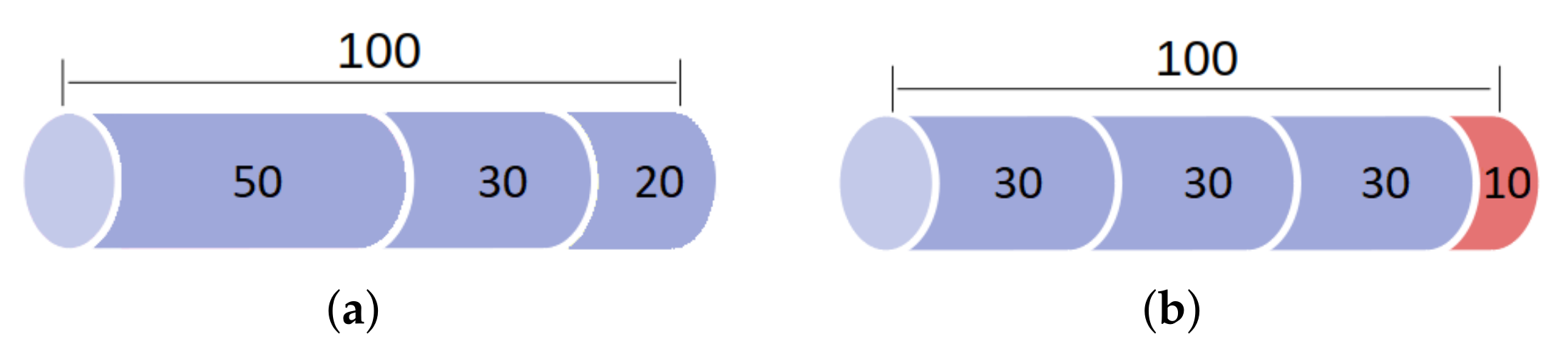
In the running example, there exist $n=7$ cutting patterns, depicted in the search tree, from left to right: $a_1={(2,0,0)}^T$, $a_2={(1,1,1)}^T$, $a_3={(1,0,2)}^T$, $a_4={(0,3,0)}^T$, $a_5={(0,2,2)}^T$, $a_6={(0,1,3)}^T$ e $a_7={(0,0,5)}^T$. The patterns $a_2$ and $a_4$ are illustrated in Figure 3a,b, respectively.

The number n of cutting patterns can grow exponentially according to the number m of item types, and, therefore, the large number of cutting patterns generally makes computation infeasible. To cope with this issue, we propose to limit the generation to a maximum number M of cutting patterns. More precisely, a maximum number ${\mu }_i$ of cutting patterns beginning with a given type of item i is computed as follows:

$${\mu }_i=⌊M\times \frac{m-i+1}{X}⌋,whereX=\sum _{i=1}^{m}i.$$

The recursive procedure to construct the search tree follows a depth-first strategy and includes the branches of a given node according to the ordering of the items. A new branch is added only if the ${\mu }_i$ limit has not been reached for patterns beginning with type of item i.

In the running example, consider the value of $M=6$. As we have $m=3$, $X=1+2+3=6,{\mu }_1=\lfloor 6\times (3-1+1)/6\rfloor =3,{\mu }_2=\lfloor 6\times (2-1+1)/6\rfloor =2,{\mu }_3=\lfloor 6\times (1-1+1)/6\rfloor =1$. In Figure 2, only the cutting patterns represented in solid lines are actually generated in the search tree. The branch represented in dashed lines is, in turn, pruned down. In this example, the cutting patterns $a_6$ is discarded.

3.2. Application of the Generate-and-Solve

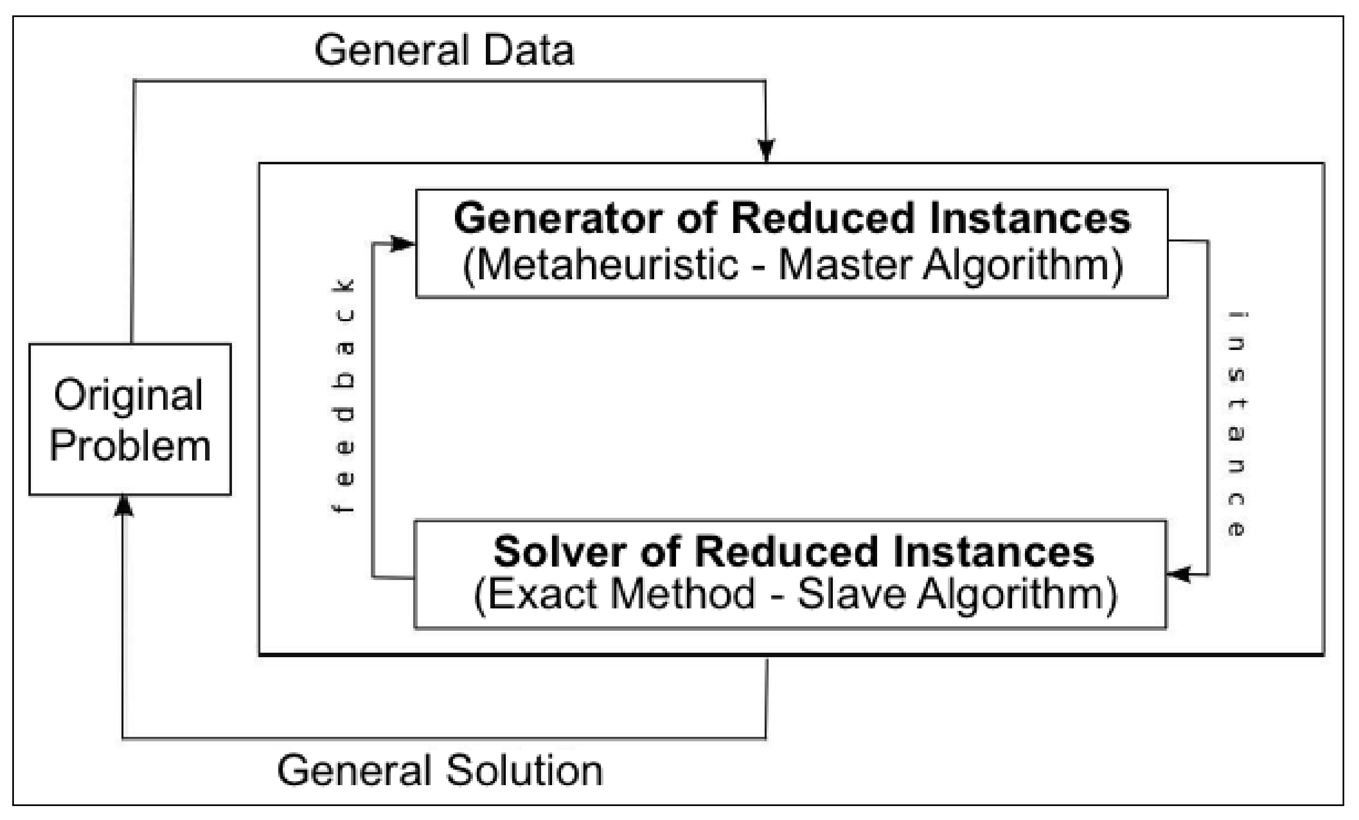
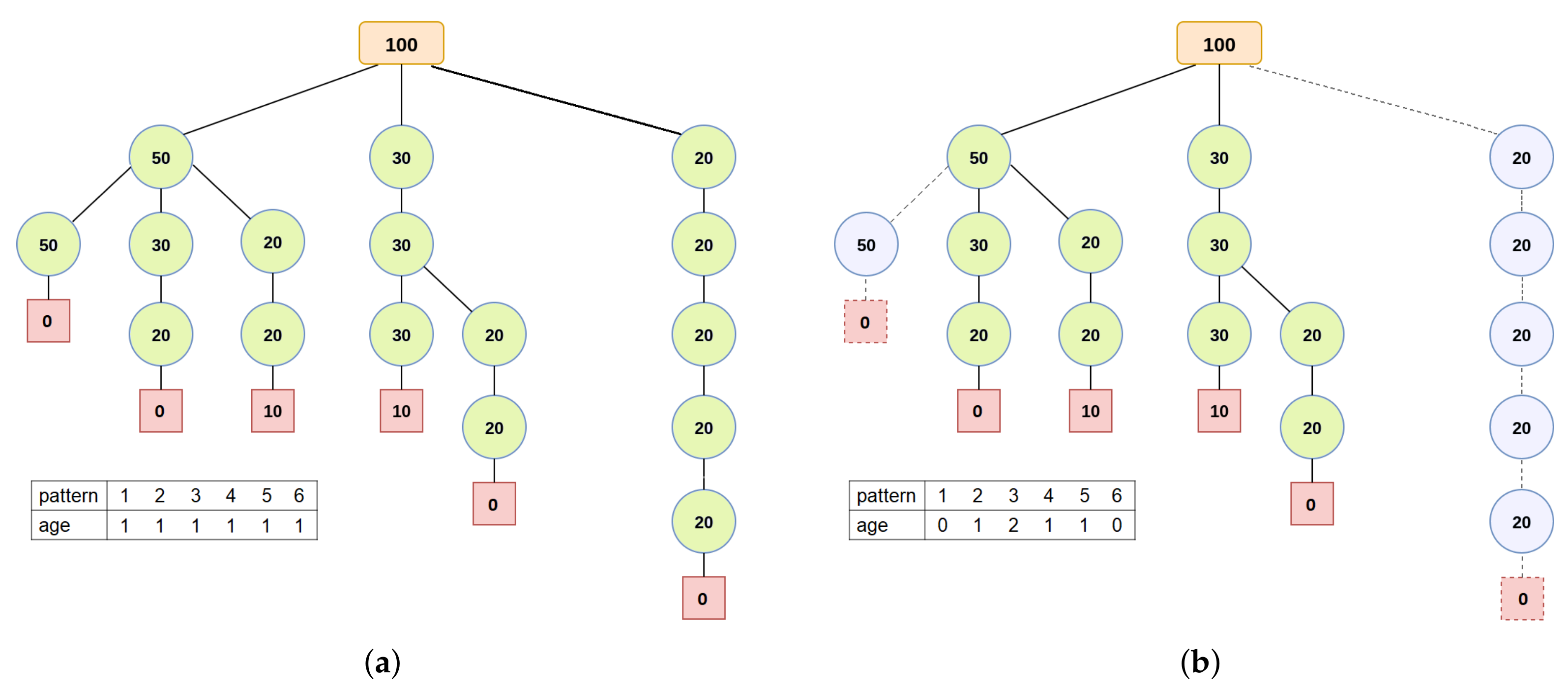
Reduced instances of the 1D-CSP can be obtained by considering only a subset of the decision variables of the original problem instance, that is, only a subset of the feasible cutting patterns. The reduced instance is, therefore, an ILP model containing all the constraints present in the problem formulation, but only a subset of the cutting patterns, as in the CG technique. The choice of the subset of cutting patterns, however, is performed through a metaheuristic engine.

To explain the representation of a reduced instance, we refer to the running example discussed previously. Recall that, in order to deal with large sized instances of the problem, we employ a strategy for reducing the number of patterns. Thus, in Figure 4, we represent only the cutting patterns that were not discarded when applying this strategy.

The representation of a reduced instance of the problem is performed using an array of integers. Each position in the array is associated with a cutting pattern in the search tree. In this representation, a value greater than or equal to 1 (one) indicates that the associated cutting pattern (decision variable) is considered in the reduced instance (ILP model). Conversely, a value of 0 (zero) indicates that the associated cutting pattern is not taken into account in the reduced instance.

In addition, the value is used as an aging mechanism [25] to control the growth of reduced instances. Whenever a new cutting pattern is incorporated into the reduced instance, its age is set to 1 (one) and, at each iteration of the G&S method, the age of every cutting pattern that is part of the reduced instance is increased by 1 (one). If the age of a cutting pattern reaches a maximum age value $\alpha$, the value is reset to 0 (zero), that is, the pattern is removed from the reduced instance to prevent unpromising cutting patterns from unnecessarily impacting the efficiency of the ILP solver. However, whenever a cutting pattern is effectively used in the solution returned by the ILP solver, its age is reset to 1 (one) to ensure that this pattern is considered in the next $\alpha$ iterations of the G&S method.

In order to obtain an initial reduced instance that produces a feasible solution when submitted to the ILP solver, the following greedy strategy was adopted to select the cutting patterns. Considering the cutting pattern search tree from left to right, the current cutting pattern is added to the instance under construction if it contains an item that has not yet been covered by any other pattern. The process continues until all items have been covered by the patterns added to the instance. Then, the reduced instance is submitted to the SRI to obtain an initial solution. From then on, the aging mechanism guarantees the existence of a feasible solution in all reduced instances submitted to the SIR. In addition, at each iteration of the G&S method, the current instance contains a solution that is at least as good as the previous ones.

For the GRI, a simple hill climbing algorithm was implemented, as illustrated in Algorithm 1. A neighbour instance is obtained from the application of a mutation operator. Considering a mutation rate $\rho$, the mutation operator, when effectively applied to a position of the array, modifies the value to 1 (one) whenever the original value is 0 (zero), and, conversely, modifies the value to 0 (zero) whenever the original value is greater than 1 (one). Note that, when the original value is 1 (one), the value remains unchanged in order to ensure that the neighbour instance preserves the current feasible solution.

Algorithm 1: Pseudocode of the generate-and-solve method implemented.

parameters: G&S time limit ${\tau }_{G\&S}$, solver time limit ${\tau }_{solver}$, maximum age value $\alpha$, and mutation rate $\rho$. input: Set of cutting patterns and demands of each type of item. output: The number of objects cut according to each cutting pattern.

At each iteration of the G&S method, a new reduced instance is generated and submitted to the SRI to obtain a new best solution. For each reduced instance, we adopt a time limit ${\tau }_{solver}$ of computation of the ILP solver. Furthermore, we consider an execution time limit ${\tau }_{G\&S}$ as a stopping criterion for the G&S method.

4. Results

We employed IBM ILOG CPLEX 22.1 [11] to solve the ILP models and used Coluna 0.4.2 (JuMP 1.1.0 and Julia 1.8) [12] to run the CG technique. Coluna implements a default CG procedure and provides dual and primal bounds for each iteration of the method. We set CPLEX as underlying ILP solver to handle master and subproblem. For the search tree, we considered a maximum number $M=\mathrm{1,000,000}$ of cutting patterns. The hill climbing algorithm was implemented in Java language and, after preliminary tests, the values of the parameters of the G&S method were chosen: ${\tau }_{G\&R}=600$ s, ${\tau }_{solver}=10$ s, $\rho =10\%$, and $\alpha =2$. The computational experiments were performed on Intel Core i7 7500U CPU 2.70 GHz 8 GB RAM machines. Benchmark instances from the literature [3], divided into 5 classes, were used to carry out a comparative analysis of the performance of the different methods. We set an execution timeout of 600 s for all methods.

The comparative results are presented in

Table 1. Results for the set of instances of class U.

	GG-ILP			REFLECT-ILP			CG			G&S
Instance	lb	ub	Time (s)	lb	ub	Time (s)	db	pb	Time (s)	Best	avg	ttb (s)
BPP_U09993_10007	5	5 *	0.0	5	5 *	48.2	5	5 *	0.4	5 *	5.0	1.2
BPP_U09978_10022	15	15 *	0.2	15	15 *	482.4	15	15 *	2.3	15 *	15.1	106.5
BPP_U09963_10037	25	25 *	1.2	25	25 *	103.3	25	25 *	5.1	25 *	25.0	9.4
BPP_U09948_10052	35	35 *	3.0	35	35 *	171.6	35	35 *	7.8	35*	35.0	2.8
BPP_U09933_10067	45	45 *	6.7	45	45 *	118.6	45	45*	13.0	45 *	45.0	8.6
BPP_U09918_10082	55	55 *	34.9	55	55 *	221.8	55	55 *	17.5	55 *	55.0	39.5
BPP_U09903_10097	65	65 *	42.6	65	65 *	474.0	65	65 *	27.1	65 *	65.0	179.7
BPP_U09888_10112	75	75 *	179.6	75	75 *	600.0	75	75 *	152.7	75 *	75.5	110.5
BPP_U09873_10127	85	85 *	106.1	85	85 *	433.1	85	85 *	171.9	85 *	85.6	178.7
BPP_U09858_10142	95	95 *	173.8	95	95 *	600.0	95	95 *	247.4	95 *	96.1	170.3
BPP_U09843_10157	105	107	600.0	105	105 *	553.4	105	105 *	293.7	106	106.5	134.5
BPP_U09828_10172	115	115 *	374.6	115	116	600.0	115	115 *	414.7	116	117.1	138.6
BPP_U09813_10187	125	128	600.0	125	126	600.0	125	125 *	490.5	127	127.0	52.6
BPP_U09798_10202	135	139	600.0	135	137	600.0	135	135 *	593.4	138	138.8	103.0
BPP_U09783_10217	145	148	600.0	145	146	600.0	145	163	600.0	150	150.0	87.7
BPP_U09768_10232	155	159	600.0	155	160	600.0	155	177	600.0	162	162.0	136.3
BPP_U09753_10247	165	169	600.0	165	170	600.0	164	186	600.0	173	173.9	67.5
BPP_U09738_10262	out-of-memory			175	182	600.0	174	195	600.0	185	185.6	148.8
BPP_U09723_10277	out-of-memory			185	192	600.0	183	208	600.0	197	197.0	191.8
BPP_U09708_10292	out-of-memory			195	202	600.0	193	222	600.0	209	209.0	84.5
BPP_U09693_10307	out-of-memory			205	211	600.0	203	233	600.0	220	220.6	155.1
BPP_U09678_10322	out-of-memory			215	222	600.0	212	243	600.0	232	232.0	198.5
BPP_U09663_10337	out-of-memory			225	232	600.0	222	257	600.0	243	243.8	128.5
BPP_U09648_10352	out-of-memory			root node not solved			230	267	600.0	255	255.9	91.6
BPP_U09633_10367	out-of-memory			root node not solved			240	278	600.0	267	267.2	225.9
BPP_U09618_10382	out-of-memory			root node not solved			249	287	600.0	279	279.0	102.3
BPP_U09603_10397	out-of-memory			root node not solved			254	300	600.0	289	290.7	86.8
BPP_U09588_10412	out-of-memory			root node not solved			261	311	600.0	302	302.5	212.6
BPP_U09573_10427	out-of-memory			root node not solved			267	324	600.0	314	314.2	131.2
BPP_U09558_10442	out-of-memory			root node not solved			274	330	600.0	325	325.9	183.4
BPP_U09543_10457	out-of-memory			root node not solved			276	342	600.0	337	337.4	240.1
BPP_U09528_10472	out-of-memory			root node not solved			269	355	600.0	349	349.1	158.6
BPP_U09513_10487	out-of-memory			root node not solved			280	367	600.0	361	361.0	104.2
BPP_U09498_10502	out-of-memory			root node not solved			294	378	600.0	372	372.9	158.1

* Proven optimal solutions.

,

Table 2. Results for the set of instances of class hard28.

	CG			G&S
Instance	db	pb	Time (s)	Best	avg	ttb (s)
BPP13	67	85	61.9	68	68.1	14.4
BPP14	61	61 *	44.6	62	62.0	6.9
BPP40	59	71	45.5	60	60.1	71.2
BPP47	71	71 *	32.3	72	72.0	8.3
BPP60	63	76	52.5	64	64.0	6.9
BPP119	76	92	79.7	77	77.0	36.6
BPP144	73	73 *	60.0	74	74.5	75.0
BPP175	83	83 *	55.5	84	84.0	9.4
BPP178	80	97	73.6	81	81.0	11.3
BPP181	72	87	59.6	73	73.0	12.9
BPP195	64	inf	52.2	65	65.0	32.6
BPP359	75	88	46.7	76	76.0	7.3
BPP360	62	62 *	27.4	63	63.0	8.6
BPP419	80	80 *	78.2	81	81.0	8.1
BPP485	71	87	59.7	72	72.0	6.4
BPP531	83	83 *	35.8	84	84.0	8.6
BPP561	72	86	59.6	73	73.0	121.4
BPP640	74	74 *	29.0	75	75.0	8.0
BPP645	58	58 *	37.6	59	59.0	8.6
BPP709	67	67 *	53.9	68	68.0	70.9
BPP716	75	88	32.9	76	76.0	7.1
BPP742	64	64 *	29.2	65	65.0	8.5
BPP766	62	62 *	46.3	63	63.0	7.8
BPP781	71	86	56.6	77	77.0	13.1
BPP785	68	68 *	70.8	69	69.0	50.4
BPP814	81	97	30.6	83	83.0	6.4
BPP832	60	60 *	44.8	61	61.0	8.9
BPP900	75	75 *	88.4	79	79.0	11.2

* Proven optimal solutions.

,

Table 3. Results for the set of instances of class 7hard.

	GC			G&S
Instance	db	pb	Time (s)	Best	avg	ttb (s)
BPP_10000108_0257	35	35 *	25.1	36	36.0	3.7
BPP_12000107_0894	39	39 *	21.3	40	40.0	5.8
BPP_16000108_0149	51	51 *	26.9	52	52.0	7.3
BPP_18000108_0359	63	77	34.2	64	64.0	6.5
BPP_18000108_0716	62	62 *	22.1	63	63.0	4.8
BPP_20000108_0175	59	59 *	27.6	60	60.0	7.5
BPP_20005008_0124	67	79	35.7	68	68.0	4.0

* Proven optimal solutions.

,

Table 4. Results for the set of instances of class hard10.

	CG			G&S
Instance	db	pb	Time (s)	Best	avg	ttb (s)
HARD0	55	63	600.0	56	57.6	340.6
HARD1	56	62	600.0	57	57.0	21.2
HARD2	56	63	600.0	57	58.6	175.3
HARD3	55	61	600.0	56	57.7	140.8
HARD4	56	inf	600.0	57	58.8	173.7
HARD5	55	61	600.0	56	58.6	163.6
HARD6	56	64	600.0	57	58.6	112.0
HARD7	54	61	600.0	56	56.0	13.2
HARD8	56	63	600.0	57	57.9	178.8
HARD9	55	62	600.0	56	56.7	71.3

and

Table 5. Results for the set of instances of class wae_gau1.

	CG			G&S
Instance	db	pb	Time (s)	Best	avg	ttb (s)
WAE_GAU1_TEST0005	28	inf	33.8	29	29.0	8.4
WAE_GAU1_TEST0014	23	23 *	18.9	24	24.0	4.6
WAE_GAU1_TEST0022	14	14 *	6.6	15	15.0	2.4
WAE_GAU1_TEST0030	27	27 *	28.9	28	28.0	4.9
WAE_GAU1_TEST0044	14	14 *	13.6	15	15.3	133.9
WAE_GAU1_TEST0049	11	inf	6.7	12	12.0	185.7
WAE_GAU1_TEST0054	14	inf	12.6	15	15.0	167.4
WAE_GAU1_TEST0055	15	inf	11.9	16	16.3	133.8
WAE_GAU1_TEST0055_2	20	inf	12.1	22	22.1	112.9
WAE_GAU1_TEST0058	20	inf	15.5	20 *	20.7	89.3
WAE_GAU1_TEST0065	15	19	6.8	16	16.0	1.4
WAE_GAU1_TEST0068	12	inf	7.2	13	13.0	74.5
WAE_GAU1_TEST0075	13	inf	7.0	14	14.1	48.8
WAE_GAU1_TEST0082	24	inf	10.2	24 *	24.9	11.3
WAE_GAU1_TEST0084	16	inf	17.7	16 *	16.5	120.8
WAE_GAU1_TEST0095	16	inf	15.3	17	17.3	162.3
WAE_GAU1_TEST0097	12	inf	10.7	13	13.0	15.5

* Proven optimal solutions.

. Along with the characterisation of the instances, we present the computational results for the different methods. Since G&S is stochastic, we provide the best and average values over 10 (ten) executions of this method, besides the average time to best ($ttb$), i.e., the elapsed time until finding the best solution of an execution. For the CG algorithm, we provide the dual lower bound $\left(db\right)$ and the primal upper bound $\left(pb\right)$. Note that, when the CG algorithm stops before convergence due to the time limit of 600 s, the dual bound may not represent the object value of the linear relaxation of the original ILP formulation. For each instance, we mark the proven optimal solutions with the symbol ${}^{*}$ and highlight in boldface the best solutions found among those obtained by the competitive approaches. Particularly, in Table 1, we present as well computational results for the ILP formulations proposed by Gilmore and Gomory [5,6] (GG-ILP) and Delorme and Iori [18] (REFLECT-ILP), in an attempt to investigate the scalability of the exact approach. In this table, $lb$ and $ub$ define, respectively, a primal lower bound and a primal upper bound for the ILP models.

The computational results for the set of instances of class U are presented in Table 1. The characteristics of these instances are as follows: the number of types of items ranges from 15 to 1005; the length of each item is between 31.66% and 35.01% of the length of the object; and the demand multiplicity (i.e., the average demand per item type), calculated as the average value among all instances of the class, is unitary. CPLEX was able to obtain feasible solutions to the GG-ILP formulation only for the instances with up to 495 item types. For the small sized instances, GG-ILP obtained proven optimal solutions very fast. The REFLECT-ILP, in turn, obtained feasible solutions for the instances with up to 675 item types. Despite the fact that REFLECT-ILP proved to be more time consuming for small sized instances compared to GG-ILP, CPLEX scaled better with this formulation. CG and G&S methods were able to find feasible solutions for all instances of this class. CG proved to be the most effective and time efficient for small sized instances (with up to 405 item types). It is important to remark that, for medium sized instances, CG outperforms the G&S approach. G&S obtained optimal solutions for instances with up to 285 item types. In addition, for large sized instances, G&S provided the best feasible solutions, and, therefore, the strategy of artificially limiting the number of cutting patterns proved to be very effective.

The set of instances of class hard28, presented in Table 2, has between 136 to 189 types of items. In these instances, the length of each item is between 0.1% and 80.0% of the length of the object and the demand multiplicity is of 1.1221. The demands vary from 1 (one) to 3 (three). The wide variety of the length of the items in relation to the length of the object stands out. CG method obtained the proven optimal solution for 15 out of 28 instances. This method, however, was not able to provide a feasible solution for the instance BPP195, which does not have any particular characteristic that justifies this behavior. Conversely, G&S obtained a better solution for 13 out of 28 instances of this class. For the other instances (but instance BPP900), the difference in the quality of the solution obtained by the G&S approach and the proven optimal solution was limited to 1 (one) additional object. It is also important to remark that the elapsed time until finding the best solution is relatively small, suggesting that convergence was reached very fast.

In Table 3, the computational results for the set of instances of class 7hard are presented. These instances are characterised by: number of types of items ranging from 85 to 143; length of each item is between 1.7% and 80.0% of the length of the object; and demand multiplicity is of 1.1027 units per item (varying from 1 to 4). As in the set of instances of class hard28, there is a wide variety of the length of the items, although the ratio for the smallest length is a little larger. Note, also, that the number of types of items is smaller here. For these instances, CG method provided the proven optimal solution for 5 instances. G&S obtained a better solution for 2 out of 7 instances of this class. Again, for the other 5 instances, the quality of the solution obtained by the G&S approach and the proven optimal solution differs by 1 (one) additional object. The convergence of both algorithms is very fast.

The set of instances of class hard10, presented in Table 4, has between 197 and 200 types of items. In these instances, the length of each item is between 20% and 35% of the length of the object and the demand multiplicity is of 1.0050 units per item (varying from 1 to 3). The number of types of items is greater than in the two previous classes, but there is a significantly smaller variation in the length of the items. For all instances of this class, G&S overachieved the CG method and the solutions differed by 1 (one) additional object considering the dual lower bound provided by the CG algorithm (but for instance HARD7). It was also noticed that CG was not able to obtain a feasible solution for the instance HARD4.

Finally, the computational results for the set of instances of class wae_gau1 are presented in Table 5. These instances are characterised by: the number of types of items ranges from 33 to 64; the length of each item is between 0.02% and 73.32% of the length of the object; and the demand multiplicity is of 2.5974 (varying from 1 to 38). The number of items is lower in relation to the other classes of instances, but with a large demand multiplicity. In addition, the variation in the length of the items is huge. For these instances, G&S significantly outperformed CG. The solutions obtained by the G&S method differed at most by 1 (one) from the lower bound provided by the CG algorithm (but, for instance, WAE_GAU1_TEST0055_2). In fact, the CG method was only able to handle 4 out 17 instances of this class. Again, the strategy of artificially limiting the number of cutting patterns proved to be effective.

5. Conclusions

The computational effort for solving the 1D-CSP is largely affected by the number of the cutting patterns. In order to cope with large instances of the problem, we proposed a strategy to restrict the number of patterns to be generated while applying a pattern generating procedure. Using benchmark instances, computational experiments were performed for ILP models, an implementation of the CG technique, and an application of the G&S framework. We begin the conclusions on our experimental analysis, stating that the exact approach was only able to cope well with small and medium-sized instances. In addition, none of the CG and G&S algorithms stood out from the other for all instances. In fact, the effectiveness of these methods varied according to the characteristics of the instances, such as the number of item types, the size of the items in relation to the size of the object, and the demand multiplicity. Nonetheless, G&S performed well for all classes, obtaining quasi-optimal solutions for the majority of the instances. In addition, the strategy of artificially reducing the number of cutting patterns proved to be very effective.

It is important to remark, however, that G&S does not present any sort of guarantee of convergence and the optimality gap cannot be estimated by the G&S method alone. On the other hand, CG was able to produce strong lower bounds fast. Therefore, G&S could be integrated to CG to speed up the convergence of branch-and price algorithms, especially when CG fails to produce good-quality integer feasible solutions. Future research is also envisaged to adapt the proposed framework using arc-flow formulations, which have shown to be appealing in branch-and-price algorithms.

References

1. Sweeney, P.E.; Paternoster, E.R. Cutting and Packing Problems: A Categorized, Application-Orientated Research Bibliography. J. Oper. Res. Soc. 1992, 43, 691–706. [Google Scholar] [CrossRef]
2. Arai, H.; Haraguchi, H. A Study of Ising Formulations for Minimizing Setup Cost in the Two-Dimensional Cutting Stock Problem. Algorithms 2021, 14, 182. [Google Scholar] [CrossRef]
3. ESICUP: Working Group on Cutting and Packing. Data Sets. Available online: https://www.euro-online.org/websites/esicup (accessed on 11 September 2022).
4. Dantzig, G.B.; Wolfe, P. Decomposition Principle for Linear Programs. Oper. Res. 1960, 8, 101–111. [Google Scholar] [CrossRef]
5. Gilmore, P.C.; Gomory, R.E. A Linear Programming Approach to the Cutting-Stock Problem. Oper. Res. 1961, 9, 849–859. [Google Scholar] [CrossRef] [Green Version]
6. Gilmore, P.C.; Gomory, R.E. A Linear Programming Approach to the Cutting Stock Problem—Part II. Oper. Res. 1963, 11, 863–888. [Google Scholar] [CrossRef]
7. Nepomuceno, N.; Pinheiro, P.R.; Coelho, A.L. Tackling the container loading problem: A hybrid approach based on integer linear programming and genetic algorithms. In Proceedings of the European Conference on Evolutionary Computation in Combinatorial Optimization, Valencia, Spain, 11–13 April 2007; Springer: Berlin, Germany, 2007; pp. 154–165. [Google Scholar] [CrossRef]
8. Nepomuceno, N.; Pinheiro, P.R.; Coelho, A.L. A Hybrid Optimization Framework for Cutting and Packing Problems. In Recent Advances in Evolutionary Computation for Combinatorial Optimization; Springer: Berlin, Germany, 2008; pp. 87–99. [Google Scholar] [CrossRef]
9. Saraiva, R.D.; Nepomuceno, N.; Pinheiro, P.R. The generate-and-solve framework revisited: Generating by simulated annealing. In Proceedings of the European Conference on Evolutionary Computation in Combinatorial Optimization, Vienna, Austria, 3–5 April 2013; Springer: Berlin, Germany, 2013; pp. 262–273. [Google Scholar] [CrossRef]
10. Dias Saraiva, R.; Nepomuceno, N.; Rogério Pinheiro, P. A Two-Phase Approach for Single Container Loading with Weakly Heterogeneous Boxes. Algorithms 2019, 12, 67. [Google Scholar] [CrossRef] [Green Version]
11. Cplex, I.I. 12.8 User’s Manual. In Book 12.8 User’s Manual, Series 12.8 User’s Manual; IBM: Armonk, NY, USA, 2017. [Google Scholar]
12. Marques, G.; Vanderbeck, F. Coluna: An Open-Source Branch-Cut-and-Price Framework. Available online: https://github.com/atoptima/Coluna.jl (accessed on 11 September 2022).
13. Kantorovich, L.V. Mathematical Methods of Organizing and Planning Production. Manag. Sci. 1960, 6, 366–422. [Google Scholar] [CrossRef]
14. Wäscher, G.; Haußner, H.; Schumann, H. An improved typology of cutting and packing problems. Eur. J. Oper. Res. 2007, 183, 1109–1130. [Google Scholar] [CrossRef]
15. Delorme, M.; Iori, M.; Martello, S. Bin packing and cutting stock problems: Mathematical models and exact algorithms. Eur. J. Oper. Res. 2016, 255, 1–20. [Google Scholar] [CrossRef]
16. Scheithauer, G.; Terno, J. The modified integer round-up property of the one-dimensional cutting stock problem. Eur. J. Oper. Res. 1995, 84, 562–571. [Google Scholar] [CrossRef]
17. Valério de Carvalho, J. Exact solution of bin-packing problems using column generation and branch-and-bound. Ann. Oper. Res. 1999, 86, 629–659. [Google Scholar] [CrossRef]
18. Delorme, M.; Iori, M. Enhanced Pseudo-polynomial Formulations for Bin Packing and Cutting Stock Problems. INFORMS J. Comput. 2020, 32, 101–119. [Google Scholar] [CrossRef] [Green Version]
19. Valério de Carvalho, J. LP models for bin packing and cutting stock problems. Eur. J. Oper. Res. 2002, 141, 253–273. [Google Scholar] [CrossRef]
20. Ben Amor, H.; Desrosiers, J.; Valério de Carvalho, J.M. Dual-Optimal Inequalities for Stabilized Column Generation. Oper. Res. 2006, 54, 454–463. [Google Scholar] [CrossRef]
21. Clautiaux, F.; Alves, C.; Valério de Carvalho, J.; Rietz, J. New Stabilization Procedures for the Cutting Stock Problem. INFORMS J. Comput. 2011, 23, 530–545. [Google Scholar] [CrossRef] [Green Version]
22. Scheithauer, G.; Terno, J.; Müller, A.; Belov, G. Solving one-dimensional cutting stock problems exactly with a cutting plane algorithm. J. Oper. Res. Soc. 2001, 52, 1390–1401. [Google Scholar] [CrossRef]
23. Belov, G.; Scheithauer, G. A branch-and-cut-and-price algorithm for one-dimensional stock cutting and two-dimensional two-stage cutting. Eur. J. Oper. Res. 2006, 171, 85–106. [Google Scholar] [CrossRef]
24. Blum, C.; Raidl, G.R. Hybridization Based on Problem Instance Reduction. In Hybrid Metaheuristics: Powerful Tools for Optimization; Springer: Cham, Switzerland, 2016; pp. 45–62. [Google Scholar] [CrossRef]
25. Blum, C.; Pinacho, P.; López-Ibáñez, M.; Lozano, J.A. Construct, Merge, Solve & Adapt: A new general algorithm for combinatorial optimization. Comput. Oper. Res. 2016, 68, 75–88. [Google Scholar] [CrossRef]
26. Hussain, K.; Mohd Salleh, M.N.; Cheng, S.; Shi, Y. Metaheuristic research: A comprehensive survey. Artif. Intell. Rev. 2019, 52, 2191–2233. [Google Scholar] [CrossRef] [Green Version]
27. Archetti, C.; Speranza, M. A survey on matheuristics for routing problems. EURO J. Comput. Optim. 2014, 2, 223–246. [Google Scholar] [CrossRef] [Green Version]
28. Ball, M.O. Heuristics based on mathematical programming. Surv. Oper. Res. Manag. Sci. 2011, 16, 21–38. [Google Scholar] [CrossRef]
29. Doerner, K.F.; Schmid, V. Survey: Matheuristics for Rich Vehicle Routing Problems. In Proceedings of the Hybrid Metaheuristics, Vienna, Austria, 1–2 October 2010; Blesa, M.J., Blum, C., Raidl, G., Roli, A., Sampels, M., Eds.; Springer: Berlin/Heidelberg, Germany, 2010; pp. 206–221. [Google Scholar] [CrossRef]
30. Monaci, M.; Toth, P. A Set-Covering-Based Heuristic Approach for Bin-Packing Problems. INFORMS J. Comput. 2006, 18, 71–85. [Google Scholar] [CrossRef] [Green Version]
31. Suliman, S.M. Pattern generating procedure for the cutting stock problem. Int. J. Prod. Econ. 2001, 74, 293–301. [Google Scholar] [CrossRef]
Figure 1. Generate-and-solve framework.
Algorithms 15 00394 g001
Figure 2. Example of a cutting pattern search tree.
Algorithms 15 00394 g002
Figure 3. Examples of cutting patterns. The items are drawn in blue and the cut loss is drawn in red. In (a), we illustrate the cutting pattern a 2 with cut loss equal to 0 and, in (b), the cutting pattern a 4 with cut loss equal to 10.
Algorithms 15 00394 g003
Figure 4. In the representation of reduced instances of the problem, each position in the array is associated with a cutting pattern in the search tree. The cutting patterns considered in the reduced instance present a value greater than or equal to 1 (one) in the array and are highlighted in green in the search tree. In (a), we illustrate a reduced instance with all cutting patterns from the search tree and, in (b), a reduced instance with only 4 cutting patterns.
Algorithms 15 00394 g004