MIRROR: Methodological Innovation to Remodel the Electric Loads to Reduce Economic OR Environmental Impact of User

Abstract

Demand for electricity is constantly increasing, and production is facing new constraints due to the current world situation. An alternative to standard energy production methodologies is based on the use of renewable sources; however, these methodologies do not produce energy consistently due to weather factors. This results in a significant commitment of the user who must appropriately distribute loads in the most productive time slots. In this paper, a comparison is made between two methods of predicting solar energy production, one statistical and the other meteorological. For this work, a system capable of presenting the scheduling of household appliances is tested. The system is able to predict the energy consumption of the users and the energy production of the solar system. The system is tested using data from three different users, and the mean percentage of consumption reduction is about 77.73%. This is achieved through optimized programming of appliance use that also considers user comfort.

1. Introduction

The electricity demand is increasing rapidly, and this has triggered the inevitable increase in the price of electricity due to economic, environmental, geopolitical, and social factors [1]. In Italy, where coal is still very present in the production of electricity, the nation, for the seventh consecutive year, was able to exceed the 17% target, set by the European Commission for 2020, for the share of renewable energy sources (RES share) on total consumption, reaching a value of 21.5 M toe and coverage of around 20% [2]. The spread of photovoltaic (PV) systems has enabled, potentially, each family to be a prosumer (i.e., a producer and user). At the same time, PV is not sufficient to be a stand-alone solution. The correct direction must include optimizing consumption. An example is the work of Iqbal et al. [3], where the energy storage system (ESS) and the PV system were modeled in order to compute the optimal scheduling of the household appliance. This type of system is part of the home energy management system (HEMS), and the HEMS could help to achieve more economically efficient use of electricity [4]. Hence, smart houses could reduce the peak energy demands by shifting the loads, and the collaboration between HEMS and the energy providers could decrease the electricity consumption costs [4]. HEMS should be considered as a solution to the Sustainability Development Goals (SDGs). The SDGs are goals established by the United Nations (UN) in order to lead several nations in the UN to sustainable development to reduce pollution, to increment equality, to ensure intra- and inter-generational justice, and to achieve the reduction of the global temperature. The focus is on the seven SDGs called “Ensure access to affordable, reliable, sustainable and modern energy for all”. Specifically, the results carried by this work could be an improvement of goal 7.2 “By 2030, increase substantially the share of renewable energy in the global energy mix” because optimization of household appliance scheduling could lead to a reduction of billing costs and a reduction in the power demands on the supply system.

This work proposes a novel and integrated system able to compute new scheduling for household load usage without affecting customer comfort. Hence, the proposed system increases energy efficiency by making full use of renewable energy resources. In this regard, a comparison between two methods to predict power production is presented in order to select the best method to achieve lower billing costs.

This paper is organized as follows. Section 2 provides the literature review. Section 3 explains extensively the methods used to build the systems; Section 4 concerns the dataset used to build the experiments; and Section 5 presents the experiments and their results. Finally, the conclusions are presented in Section 6.

2. Related Works

The topic of energy efficiency within smart grids or home energy management systems (HEMS) has been frequently explored in recent years. Energy efficiency can be achieved using optimization techniques. These techniques are used to find the best solution in the search space, or otherwise an optimal solution, by evaluating it with an objective function and some constraints. Energy efficiency is a very mature and broad field of research. Panagiotis et al. proposed in [5] a real-time energy management system for a smart hybrid power system for base transceivers. In this way, the authors of [5] reduced the Base Transceiver Station (BTS) operational costs. The focus of cellular operators was also shifted to the use of renewable energies, such as solar or wind energy. In fact, in [6], authors have considered a green base station. The authors in [6] have modeled the problem as a Markov decision problem and the authors have discovered the existence of a stationary average-cost optimal policy. In [7], an evaluation of the performance of different types of base stations was done. This evaluation was based on considering a cellular base station network. Hence, in [7], the authors have highlighted the advantages of using renewable energy systems (RES) and the need to have a plan for the (RES) system in order to reduce or eliminate power supply outages (this is a problem related to renewable energy due to natural conditions, such as cloudiness, which impact solar power production). Moreover, in [7] authors highlighted that an accurate usage of fuel generators could significantly impact the OPEX (Operational Expenditure; it is the energy consumption of radio base stations) reduction and the CO₂ reduction. In recent years, the idea to use renewable energy along with energy storage systems was explored by different works. Yohwan C. and Hongseok K. proposed in [8] a multi-functional framework that also considers an optimal charging/discharging scheduling for the ESS. As a result, the authors achieved a reduction in the total cost and battery wear out. Ping-Huan Kuo and Chiou-Jye Huang propose a new method for performing consumption predictions called DeepEnergy [9]. It is based on the use of a convolutional neural network (CNN). The adopted dataset is a public one provided by the Texas Electric Reliability Council, consisting of public consumption data and electrical load data for the year 2016. In the experiment, the training data is about two months of recorded data, while the test data is about one month of recorded data. Following the experimental results shown in the work of Ping-Huan Kuo and Chiou-Jye Huang [9], DeepEnergy can accurately predict the energy load in the next three days. In addition, the proposed algorithm was compared with five commonly used algorithms for load prediction. The comparison showed that DeepEnergy’s performance is the best and has the lowest mean absolute percentage error (MAPE) and coefficient of the variation of the root mean square error (CV-RMSE) values. Rodrigues et al. [10] proposed an artificial neural network (ANN) intending to predict the energy load in the short term. Short-term is defined as a daily or hourly prediction. Hence, the data used are hourly and daily information on the energy consumed. The extension of the apartment or the number of inhabitants is also considered to achieve a robust prediction model. This type of model could also be useful in the design phases of energy storage systems, and the design of renewable energy systems. An interesting work by Xu et al. [11] presents a reinforcement learning model in order to predict the future trend of electricity costs and the energy produced by photovoltaic panels. The reinforcement model is based on the use of a feedforward NN and a Q-learning algorithm. The results show that the proposed model can reduce the electricity costs for household appliances and improve computational costs.

M.M. Iqbal et al. proposed the use of a genetic algorithm (GA) to reschedule the household appliance accordingly with information on energy storage systems (ESS) and photovoltaic (PV) generation [12]. In this way, the system could choose to export, import, or store energy in order to reduce energy demands and costs. The same authors also presented the use of a Grey Wolf optimization algorithm to reduce the overall electricity cost, improve the performance of home electricity scheduling, and decreasing the effect of the uncertainty of the data. In their work [3], Iqbal et al. [13] also proposed the use of a stochastic model in order to learn and predict solar power production, simulate the energy storage system behavior, and schedule household appliance usage. The authors of [3], proposed a novel optimization technique to reduce the energy costs that imply a reduction of the energy demands from the energy provider. The technique is the fusion of the Grey Wolf algorithms with the genetic algorithm. A. Khalid et al. presented in [14] an attempt to coordinate the switching on and off of electronic devices through a load-shifting strategy approach for users with a time slot contract, trying not to affect the habits and comforts of the user. The system allows programming that takes place the day before and, if necessary, even programming in real-time. The work compares different optimization algorithms based on the application domain, the devices in use, the limitations on the user, and the results obtained. There is the use and comparison of different optimization algorithms such as GA (genetic algorithm), BFA (bacterial foraging algorithm), and HBG (hybrid bacterial foraging). The addition of micro-plants to produce renewable energy and storage systems is not considered. S. Rahima et al. proposed an approach that solves the global optimization problem using meta-heuristic algorithms for a domestic user based on time of use (TOU) consumption [15]. A comparison is made between different algorithms: GA (genetic algorithm), BPSO (binary particle swarm optimization), and ACO (ant colony optimization algorithms). Moreover, the problem-solving strategy is approached through a multiple backpack problem (Greedy). Results show that the GA algorithm is the most efficient in comparison to the others, with the minimization of the peak-average ratio and maximization of the user’s comfort level.

This work proposes a framework in which consumption prediction and energy production prediction are used together with the modeling of an energy storage system (ESS) to propose optimal scheduling to the user. In addition, the optimal scheduling is based on the user’s consumption preferences.

The proposed framework was also compared with and without the use of meteorological information for energy production prediction. To the best of the authors’ knowledge, weather information has not been considered in any other work.

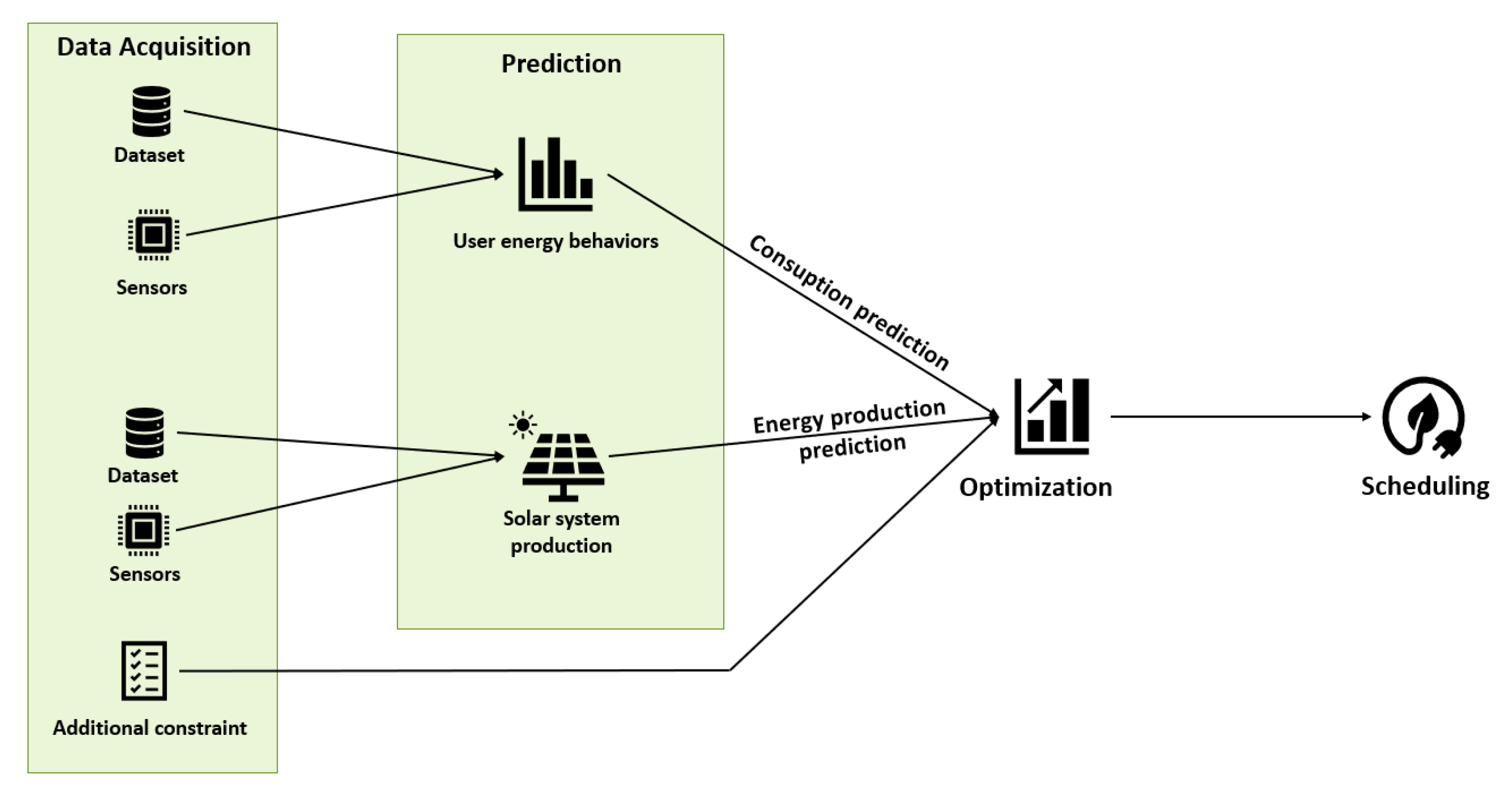
3. Methods

The overall system proposed in this work is based on the framework shown in Figure 1. It includes four computational phases: “Data Acquisition”, “Data prediction”, “Optimization”, and “Scheduling”. All these phases are explained in Section 3.1, Section 3.2, Section 3.3 and Section 3.4.

3.1. Data Acquisition

In this phase, the data acquired are heterogeneous and concerned with energy consumption, energy production from the solar system, user preferences regarding the times at which household appliances are turned on during the day, meteorological data, and additional constraints, which mean constraints such as the hourly cost of electricity derived from the user contract, storage systems (ESS), and their capacity. The hourly cost of electricity could be based on two main models: real-time pricing (RTP) or time of use (TOU) [12]. The first one consists of the kWh price, which varies according to the hour of the day. With this contract, time slots are defined, mainly three. Depending on the time slot, the price of energy varies. The latter is based on the use of a fixed price of electricity during the day. In this work, real-time pricing (RTP) was used as an energy cost setting.

3.2. Prediction

After data acquisition, the data were used to perform predictions. In this work, two types of prediction are performed, the first one is related to learning the energy consumption behavior of users in order to predict the consumption for the next 24 h. The second one aims to learn the energy production of solar systems in order to perform a prediction of the energy production for the next 24 h.

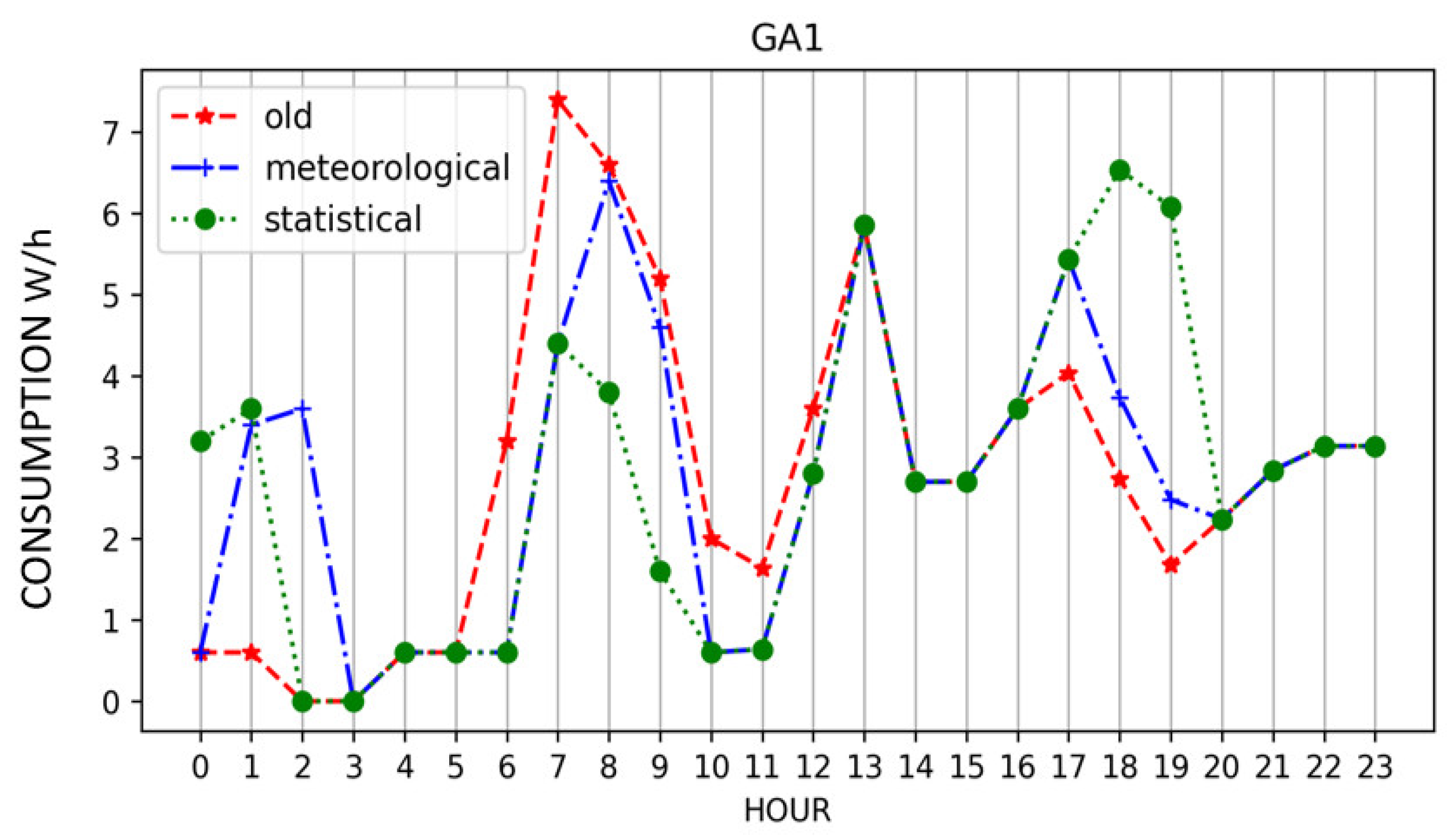
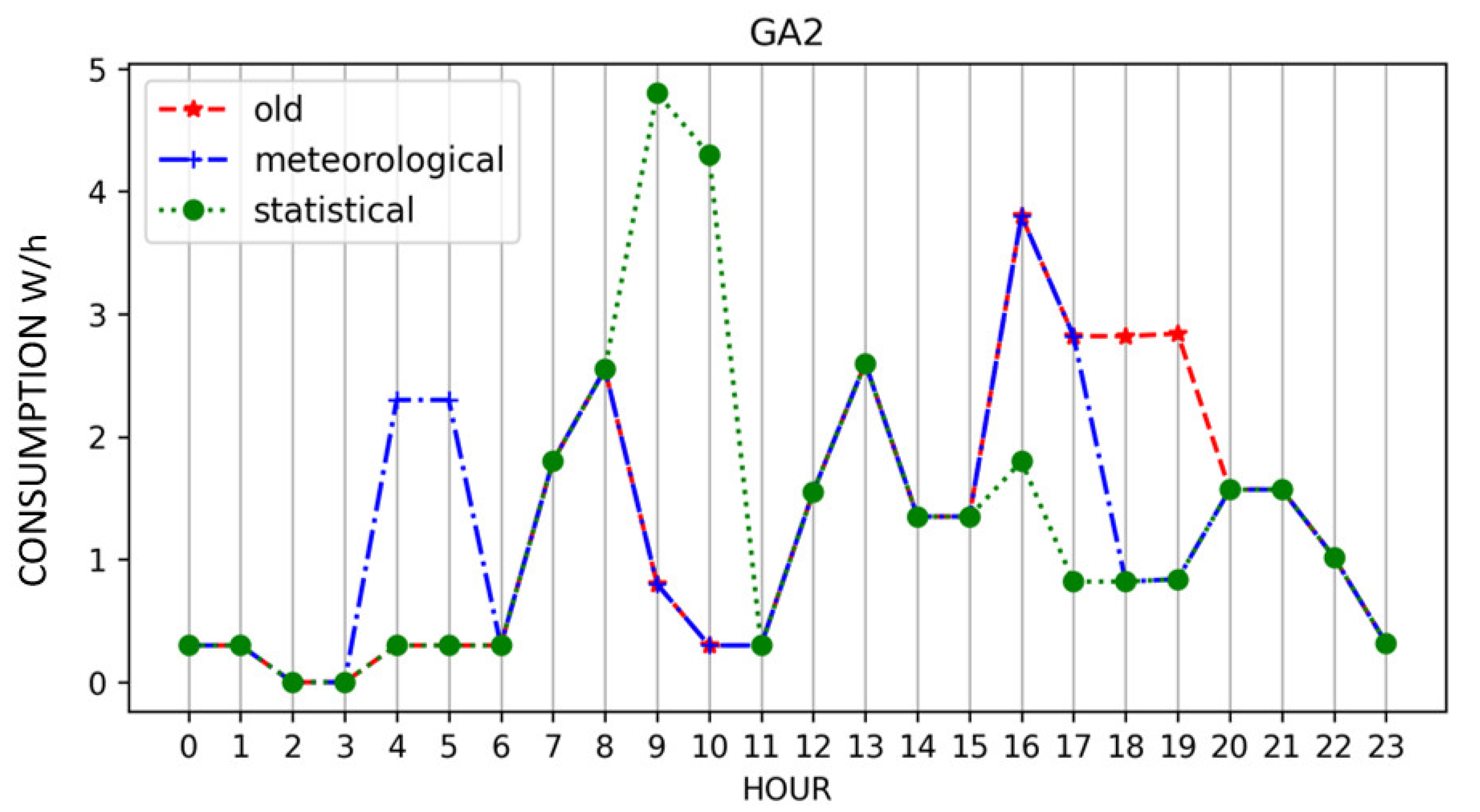
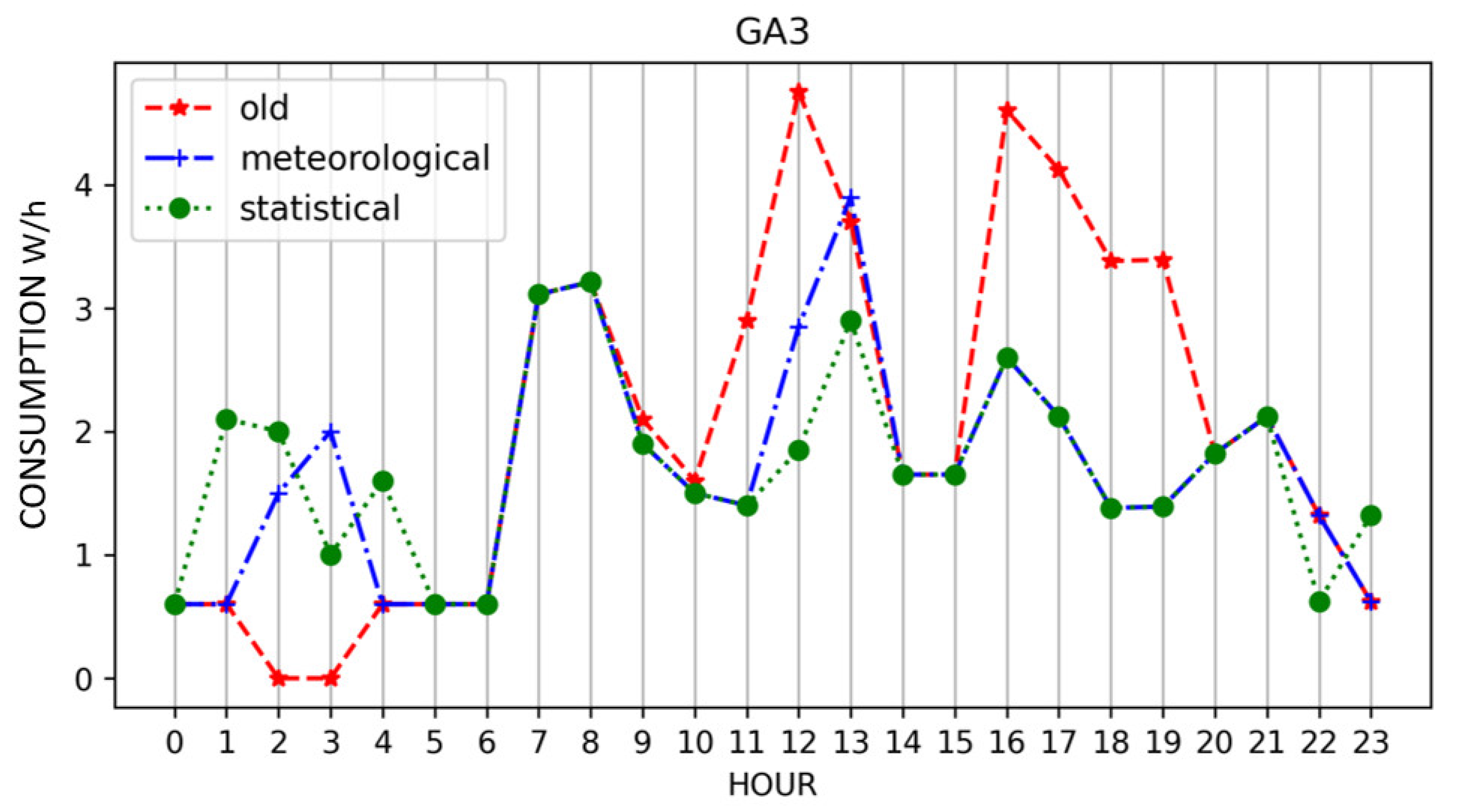
3.2.1. Consumption Prediction

According to the literature [13,16], household appliances are divided into three categories:

• devices for occasional use: all devices used when needed and not for continuous use (e.g., TV, PC, or similar).
• non-interruptible devices: all devices that cannot be interrupted and require continuous use of current, or are independent of the user’s use (e.g., refrigerators, lighting, alarms).
• interruptible devices (shiftable): all devices that can be interrupted and used later, or programmed (e.g., dishwashers, washing machines, or other smart appliances).

The time of use of many devices, both occasional and interruptible types, depends on the habits and needs of the users, while for non-interruptible devices this does not apply. Instead, the time of use is influenced by the season (winter or summer seasons). In this work, each device can be used simultaneously or deferred with other devices over the course of the day, 24 h. Moreover, the kWh consumption of household appliances has been computed according to the literature [14,15,17] in order to achieve comparable values.

Different profiles of households (i.e., a person or a group of people who use electricity to power their home) can be distinguished, which will therefore have different consumption. In this paper, the term “user” (or “users”) refers to the concept of “household” (respectively “households”). Consumption depends on the number of people in the household, such as the number of devices and the frequency of use of those devices.

In the proposed system, three standard types of households have been used from the UK-DALE dataset:

• household composed of two young people (aged between 21 and 30);
• household composed of two elderly persons (with ages over 60 years);
• four-person household (with two household members included with ages between 30 and 50 years and the other two household members ages between 0 and 20 years of age).

For the consumption prediction, the SARIMAX algorithm has been used on the UK-DALE dataset. The experiments were done by conducting training over the previous 7 days and a test over the next day. The data have granularity per minute; thus, the training is performed on 10,080 values per minute (7 days) and the test is performed on 1440 values per minute (1 day).

3.2.2. Power Production Prediction

In order to make optimal consumption schedules, it is important to predict the solar energy production for the next 24 h, and this is done by modeling the global horizontal irradiance (GHI) values. In this work, two methods are used to make the GHI prediction. The first one is called “Meteorological Method” and is based, as the name suggests, on meteorological data. The second one doesn’t consider that data, and it is called “Statistical Method”. The Global Horizontal Irradiance (GHI), first calculated by the meteorological method (sub-section a.) and then by the statistical method (sub-section b.), was used to predict power production. Then the calculated production predictions were compared.

a. 

Meteorological method for GHI prediction

In the meteorological method, the solar irradiance calculated for clear sky situations in a specific area can be approximated by models that consider the solar zenith angle (the “z” parameter in Equation (1)). It has been shown in [18] that the model that best approximates the global horizontal irradiance (GHI) at the clear sky is the Adnot-Bourges-Campana-Gicquel, formulated as in (Equation (1)):

$$GHI=951.39\times cos{\left(z\right)}^{1.15}$$

(1)

The parameters 951.39 and 1.15 are regression parameters empirically calculated. The computed GHI in Equation (1) is related to the clear sky scenario (“clear sky GHI”). Then, the “measured GHI” is estimated using Equation (2) extracted from [18]

$$measured GHI=clear sky GHI\times \left(1-\alpha \times cloudines{s}^n\right)$$

(2)

Equation (2) is based on the okta of covered sky, which is a specific unit measurement used to describe the amount of cloud cover in a given location. The used coefficients α and n are the same as those in [18]. Precisely, α is 0.51 and n is 6.42.

b. 

Statistical method for GHI prediction

In the statistical method, as stated in [3], the solar irradiance can be modeled using the function of probability density Beta (Equation (3)).

$$f\left(GHI \right)=\frac{\gamma \left(\alpha +\beta \right)}{\gamma \left(\alpha \right)\gamma \left(\beta \right)}\times GHI{ }^{\left(\alpha -1\right)}\times {\left(1-GHI \right)}^{\left(\beta -1\right)}, 0<GHI \left(t\right)<\infty$$

(3)

where GHI is the solar irradiance in kW⁄m²; f(GHI) is the beta distribution function of GHI; and α, β are the parameters of the beta distribution function. As stated in [3], the parameters are computed from the mean μ and the standard deviation σ of the random variable GHI. Hence, the used formulas are:

$$\beta =\left(\frac{\mu \times \left(1+\mu \right)}{{\sigma }^2}-1\right)\times \left(1-\mu \right)$$

(4)

$$\alpha =\frac{\mu \times \beta }{1-\mu }$$

(5)

c. 

Prediction of the power production

The prediction of electricity production was mainly modeled using the model presented by Sajjad et al. [19] and reported in the next formulas. The used formulas are:

$$P_{ac}=0.92\times P_n\times GHI\times {\eta }_{DC-AC}\times \left(1-\gamma \times \mathsf{\Delta }{T}_c\right)/1000$$

(6)

where $P_n$ is the rated power of the PV system (1–100 kWp), GHI is the global irradiance on a fixed plane, ${\eta }_{DC-AC}$ is the inverter efficiency (95%), γ is the power temperature coefficient (0.007), and $\mathsf{\Delta }{T}_c$ is:

$$\mathsf{\Delta }{T}_c=\left|25-\left(T_d+\left(NOCT-20\right)\times GHI/800\right)\right|$$

(7)

where T_d is the average daytime temperature profile calculated for each day in a year, NOCT is the “Normal Operating Cell temperature” (45 °C), and GHI is the global irradiance on a fixed plane. The values used are in line with those used by [19].

3.3. Optimization

During the optimization phase, the system calculates the optimal schedule of home appliances that can be moved throughout the day. The optimization is based on the expected energy production from the solar system (previously calculated with the GHI value predicted by one of the two methods previously described, namely, the statistical or meteorological method), the user’s energy consumption and appliance usage preferences, and the amount of energy in the energy storage system (ESS).

The data described above were processed by a genetic algorithm (GA) that has the purpose of generating optimal scheduling of shiftable household appliances that will prefer the use of energy from the solar system rather than energy purchased from suppliers. The scheduling of shiftable household appliances, also called population, is first randomly generated by the algorithm, and then based on the user’s preferences. Then, from the previous population, new generations are made to identify the best solution. This is defined as the solution that maximizes the fitness function.

The fitness function used is as follows:

$$fitness=\frac{1}{C_T}$$

(8)

where:

$$E_T\left(h\right)=E_a\left(h\right)-E_{PV}\left(h\right)\pm E_{bat}\left(h\right)$$

(9)

And

$$C_T={\displaystyle \sum }_{h=0}^{23}{E}_T\left(h\right)C_e\left(h\right)$$

(10)

where:

• $E_T\left(h\right)$ is the total consumed energy in a specific hour of the day.
• $E_a\left(h\right)$ is the energy consumed by household appliances at a specific hour of the day. It is important to note that energy consumption is aggregated on an hourly basis because the raw data were sampled at a frequency of six seconds.
• $E_{PV}\left(h\right)$ is the energy produced by the photovoltaic system at a specific hour of day.
• $E_{bat}\left(h\right)$ is the energy present in the ESS at a specific hour of the day. The sign “$\pm$” in (Equation (9)) indicates that the ESS could be in discharging (+) or charging mode (−). It is important to highlight that the ESS is not charged by the energy that comes from the grid.
• $C_T$ is the total cost of energy for the day.
• $C_e\left(h\right)$ is the cost of energy for electricity at a specific hour of the day.

3.4. Scheduling

Finally, once the optimization is done, the best is proposed to the user in the form of a new schedule, i.e., for each shiftable appliance, the suggested on and off times are shown to the user, also indicating any achievable savings.

4. Dataset

In this work, two datasets have been used to perform predictions and experiments. The first one, called “UK Dale” [20], has been used to model domestic energy consumption behavior; this dataset is a collection of energy consumption by household appliances from five UK homes. In each house, the electricity demand of the whole house and the energy demand of individual household appliances were recorded at a six-second rate. In order to model hourly consumptions for this work, the data were aggregated in hourly format. The second one, the European Dataset PVGIS-SARAH 2 [21,22], has been used to model solar energy production. This dataset contains the solar radiation calculated from images of the two METEOSAT geostationary satellites that cover Europe, Africa, most of Asia, and parts of South America. In addition to these datasets, weather information from the web platform “Tomorrow.io” [23] has been used to predict solar energy production.

5. Experiments and Results

In this section, the experiments and results will be described. The experiments were carried out on the predicted data. The predictions were about household consumption and power production. The predictions of the consumption were performed using the data of the “UK Dale” dataset [20] and were carried out using the aggregated data of the household appliances. The aggregation was performed with the sum of the hourly consumption of each appliance. Three types of users were tested, as described in Section 3.2.1, which differ in age, the number of components in the user nuclei, and the number of appliances. In the following figures, there will be the daily consumption before and after the application of the optimization, with and without the use of meteorological information. Figure 2, Figure 3 and Figure 4 show the optimized household appliance scheduling. The “blue” line is about the meteorological method, meanwhile, the “green” line is about the statistical method. The “red” line is about the old scheduling. Thus, the graphs compare the old energy consumption to the optimized energy consumption (both hourly based) using the statistical method and the meteorological ones. It can be seen from Figure 2, Figure 3 and Figure 4 that the meteorological method tends to model appliance utilization similarly to normal utilization, in other words, without optimization. This behavior confirms the assumption that “time of use is influenced by season”, as written in Section 3.2.1. The scheduling of appliance usage turns out to be adapted to the habits of the households, including in the optimization of the prediction of electricity production.

In

Table 1. Energy cost comparison.

	Daily Initial Consumption (€)	Daily Optimized Consumption (Meteorological) (€)	Daily Optimized Consumption (Statistical) (€)
User 1	17.4936	8.2495	10.0484
User 2	8.1198	0.4782	0.8866
User 3	12.9331	1.7787	3.4489

, it can be seen that the use of weather information during GHI prediction and consequently power production prediction helps to find an optimal schedule that decreases the daily consumption of the household appliance and consequently the daily cost. These results are related to the fact that the meteorological data gives information that impacts on the quantity of GHI that will be present on the next day of the prediction. So, the power production prediction is more reliable and closer to reality. Meanwhile, the use of statistical information to predict power production is based on information that comes from the past and does not take into account the variation in weather status.

Indeed, the savings percentage is increased. This can be seen from the values reported in

Table 2. Saving percentage.

	Daily Savings Consumption % (Meteorological)	Daily Savings Consumption % (Statistical)
User 1	52.8428	42.556
User 2	94.1107	89.081
User 3	86.2469	73.3328
Mean Saving Percentage	77.73347	68.3233

. The savings percentage is calculated by subtracting the optimized daily consumption from the initial daily consumption. Then, the value indicating the amount of savings is divided by the initial daily consumption to obtain the savings percentage. This is done for both weather-informed and non-weather-informed optimized consumption. In addition, the percentage of consumption savings depends on the usage habits of household appliances.

In Table 2, it can be seen that the meteorological method is better than the statistical method by about 10 percent.

In

Table 3. Peak comparison between optimized and not optimized scheduling (meteorological method).

	Max Daily Peak Not Optimized (W/h)	Max Daily Peak Optimized (W/h) (Meteorological)	Difference [%]
User 1	7.40	6.40	13.51
User 2	3.8	3.8	0
User 3	4.75	3.9	17.895
User 4	7.40	6.40	13.51

and

Table 4. Peak comparison between optimized and not optimized scheduling (statistical method).

	Max Daily Peak Not Optimized (W/h)	Max Daily Peak Optimized (W/h) (Meteorological)	Difference [%]
User 1	7.40	6.54	11.62
User 2	3.8	4.8	−26.316
User 3	4.75	3.21	32.421
User 4	7.40	6.54	11.62

, there is a comparison of the peak consumption and the scheduled usage of the household appliance. Specifically, in Table 3, it can be seen that the peak comparison with the meteorological method; in Table 4, there is the peak comparison with the statistical method.

In Table 3, the column “Difference [%]” is obtained by the ratio between the difference between the max daily peak not optimized and the optimized one and the max daily peak not optimized. In this way, the percentage of saving consumption is calculated. The same is done in Table 4.

It is noticeable that the saving percentage for the meteorological method in Table 3 is equal to or higher than zero. This means that, with the meteorological information, the optimization tends to lower the maximum peak of consumption.

In Table 4, different behaviors are shown. Indeed, the maximum daily peak optimized for “User 2” is higher than the maximum daily peak not optimized. Consequently, the “Difference [%]” is negative. Probably, this is due to the power production prediction, which is statistically calculated and does not consider meteorological changes.

6. Conclusions

In this work, two methods for energy production prediction are presented. The first method uses meteorological information, and the second only statistical information. Both of these methods are integrated into a system that also considers energy consumption prediction. The system aims to propose new scheduling of households’ appliance usage to lower the energy consumption of the user and, consequently, the billing costs.

The results obtained show a significant reduction in energy consumption, along with a cost reduction of 77.73% on average for the three users, using meteorological information.

Regarding scheduling, in Figure 2, with the new scheduling based on modeling user behavior (in red), and with the new scheduling (in blue the one using weather information and in green the one modeling production without the weather information), it can be seen that moving the devices placed them at peak production times, but also based on the preferences expressed by users. In this way, the optimal scheduling achieved is based on both cost reduction and user comfort.

References

- Panwar, N.L.; Kaushik, S.C.; Kothari, S. Role of renewable energy sources in environmental protection: A review. Renew. Sustain. Energy Rev. 2011, 15, 1513–1524. [Google Scholar] [CrossRef]
- Rapporto GSE 2021 sulle Fonti rinnovabili in Italia e nelle Regioni—Federazione ANIE. Available online: https://anie.it/rapporto-gse-2021-sulle-fonti-rinnovabili-in-italia-e-nelle-regioni/ (accessed on 10 December 2022).
- Iqbal, M.M.; Sajjad, M.I.A.; Amin, S.; Haroon, S.S.; Liaqat, R.; Khan, M.F.N.; Waseem, M.; Shah, M.A. Optimal Scheduling of Residential Home Appliances by Considering Energy Storage and Stochastically Modelled Photovoltaics in a Grid Exchange Environment Using Hybrid Grey Wolf Genetic Algorithm Optimizer. Appl. Sci. 2019, 9, 5226. [Google Scholar] [CrossRef]
- Erdinc, O.; Paterakis, N.G.; Mendes, T.D.P.; Bakirtzis, A.G.; Catalao, J.P.S. Smart Household Operation Considering Bi-Directional EV and ESS Utilization by Real-Time Pricing-Based DR. IEEE Trans. Smart Grid 2014, 6, 1281–1291. [Google Scholar] [CrossRef]
- Diamantoulakis, P.D.; Ghassemi, A.; Karagiannidis, G.K. Smart hybrid power system for base transceiver stations with real-time energy management. In Proceedings of the 2013 IEEE Global Communications Conference (GLOBECOM), Atlanta, GA, USA, 9–13 December 2013; pp. 2773–2778. [Google Scholar] [CrossRef]
- Lalitha, A.; Mondal, S.; Satya Kumar, V.; Sharma, V. Power-optimal scheduling for a Green Base station with delay constraints. In Proceedings of the 2013 National Conference on Communications (NCC), New Delhi, India, 15–17 February 2013; pp. 1–5. [Google Scholar] [CrossRef]
- Lorincz, J.; Bule, I.; Kapov, M. Performance Analyses of Renewable and Fuel Power Supply Systems for Different Base Station Sites. Energies 2014, 7, 7816–7846. [Google Scholar] [CrossRef]
- Choi, Y.; Kim, H. Optimal scheduling of energy storage system for self-sustainable base station operation considering battery wear-out cost. In Proceedings of the International Conference on Ubiquitous and Future Networks, ICUFN, Vienna, Austria, 5–8 July 2016; pp. 170–172. [Google Scholar] [CrossRef]
- Kuo, P.-H.; Huang, C.-J. A High Precision Artificial Neural Networks Model for Short-Term Energy Load Forecasting. Energies 2018, 11, 213. [Google Scholar] [CrossRef]
- Rodrigues, F.; Cardeira, C.; Calado, J. The Daily and Hourly Energy Consumption and Load Forecasting Using Artificial Neural Network Method: A Case Study Using a Set of 93 Households in Portugal. Energy Procedia 2014, 62, 220–229. [Google Scholar] [CrossRef]
- Xu, X.; Jia, Y.; Xu, Y.; Xu, Z.; Chai, S.; Lai, C.S. A Multi-Agent Reinforcement Learning-Based Data-Driven Method for Home Energy Management. IEEE Trans. Smart Grid 2020, 11, 3201–3211. [Google Scholar] [CrossRef]
- Iqbal, M.M.; Sajjad, I.A.; Khan, M.F.N.; Liaqat, R.; Shah, M.A.; Muqeet, H.A. Energy Management in Smart Homes with PV Generation, Energy Storage and Home to Grid Energy Exchange. In Proceedings of the 2019 International Conference on Electrical Communication and Computer Engineering (ICECCE), Swat, Pakistan, 24–25 July 2019; pp. 1–7. [Google Scholar] [CrossRef]
- Iqbal, M.M.; Manan, A.; Ali, A.; Sohail, A. Towards an Optimal Residential Home Energy Management in Presence of PV Generation, Energy Storage and Home to Grid Energy Exchange Framework. In Proceedings of the 2020 3rd International Conference on Computing, Mathematics and Engineering Technologies: Idea to Innovation for Building the Knowledge Economy, iCoMET 2020, Sukkur, Pakistan, 29–30 January 2020; pp. 1–7. [Google Scholar]
- Khalid, A.; Javaid, N.; Guizani, M.; Alhussein, M.; Aurangzeb, K.; Ilahi, M. Towards Dynamic Coordination Among Home Appliances Using Multi-Objective Energy Optimization for Demand Side Management in Smart Buildings. IEEE Access 2018, 6, 19509–19529. [Google Scholar] [CrossRef]
- Rahim, S.; Javaid, N.; Ahmad, A.; Khan, S.A.; Khan, Z.A.; Alrajeh, N.; Qasim, U. Exploiting heuristic algorithms to efficiently utilize energy management controllers with renewable energy sources. Energy Build. 2016, 129, 452–470. [Google Scholar] [CrossRef]
- Li, S.; Yang, J.; Song, W.Z.; Chen, A. A Real-Time Electricity Scheduling for Residential Home Energy Management. IEEE Internet Things J. 2018, 6, 2602–2611. [Google Scholar] [CrossRef]
- Aslam, S.; Iqbal, Z.; Javaid, N.; Khan, Z.A.; Aurangzeb, K.; Haider, S.I. Towards Efficient Energy Management of Smart Buildings Exploiting Heuristic Optimization with Real Time and Critical Peak Pricing Schemes. Energies 2017, 10, 2065. [Google Scholar] [CrossRef]
- Nguyen, D.V.; Delinchant, B.; Dinh, B.V.; Nguyen, T.X. Irradiance forecast model for PV generation based on cloudiness web service. IOP Conf. Ser. Earth Environ. Sci. 2019, 307, 012008. [Google Scholar] [CrossRef]
- Sajjad, I.A.; Manganelli, M.; Martirano, L.; Napoli, R.; Chicco, G.; Parise, G. Net metering benefits for residential buildings: A case study in Italy. In Proceedings of the 2015 IEEE 15th International Conference on Environment and Electrical Engineering (EEEIC), Rome, Italy, 10–13 June 2015; pp. 1647–1652. [Google Scholar]
- Kelly, J.; Knottenbelt, W. The UK-DALE dataset, domestic appliance-level electricity demand and whole-house demand from five UK homes. Sci. Data 2015, 2, 150007. [Google Scholar] [CrossRef] [PubMed]
- Urraca, R.; Gracia-Amillo, A.M.; Koubli, E.; Huld, T.; Trentmann, J.; Riihelä, A.; Lindfors, A.V.; Palmer, D.; Gottschalg, R.; Antonanzas-Torres, F. Extensive validation of CM SAF surface radiation products over Europe. Remote Sens. Environ. 2017, 199, 171–186. [Google Scholar] [CrossRef] [PubMed]
- Urraca, R.; Huld, T.; Gracia-Amillo, A.; Martinez-De-Pison, F.J.; Kaspar, F.; Sanz-Garcia, A. Evaluation of global horizontal irradiance estimates from ERA5 and COSMO-REA6 reanalyses using ground and satellite-based data. Sol. Energy 2018, 164, 339–354. [Google Scholar] [CrossRef]
- T. T. C. Inc. Available online: https://app.tomorrow.io/home (accessed on 10 December 2022).