Robust Representation and Efficient Feature Selection Allows for Effective Clustering of SARS-CoV-2 Variants

Abstract

The widespread availability of large amounts of genomic data on the SARS-CoV-2 virus, as a result of the COVID-19 pandemic, has created an opportunity for researchers to analyze the disease at a level of detail, unlike any virus before it. On the one hand, this will help biologists, policymakers, and other authorities to make timely and appropriate decisions to control the spread of the coronavirus. On the other hand, such studies will help to more effectively deal with any possible future pandemic. Since the SARS-CoV-2 virus contains different variants, each of them having different mutations, performing any analysis on such data becomes a difficult task, given the size of the data. It is well known that much of the variation in the SARS-CoV-2 genome happens disproportionately in the spike region of the genome sequence—the relatively short region which codes for the spike protein(s). In this paper, we propose a robust feature-vector representation of biological sequences that, when combined with the appropriate feature selection method, allows different downstream clustering approaches to perform well on a variety of different measures. We use such proposed approach with an array of clustering techniques to cluster spike protein sequences in order to study the behavior of different known variants that are increasing at a very high rate throughout the world. We use a k-mers based approach first to generate a fixed-length feature vector representation of the spike sequences. We then show that we can efficiently and effectively cluster the spike sequences based on the different variants with the appropriate feature selection. Using a publicly available set of SARS-CoV-2 spike sequences, we perform clustering of these sequences using both hard and soft clustering methods and show that, with our feature selection methods, we can achieve higher $F_1$ scores for the clusters and also better clustering quality metrics compared to baselines.

1. Introduction

The virus that causes the COVID-19 disease is called the severe acute respiratory syndrome coronavirus 2 (SARS-CoV-2)—a virus whose genomic sequence is being replicated and dispersed across the globe at an extraordinary rate. The genomic sequences of a virus can be helpful to investigate outbreak dynamics such as spatiotemporal spread, the size variations of the epidemic over time, and transmission routes. Furthermore, genomic sequences can help design investigative analyses, drugs and vaccines, and monitor whether theoretical changes in their effectiveness over time might refer to changes in the viral genome. Analysis of SARS-CoV-2 genomes can therefore complement, enhance and support strategies to reduce the burden of COVID-19 [1].

SARS-CoV-2 is a single-stranded RNA-enveloped virus [2]. Its entire genome is characterized by applying an RNA-based metagenomic next-generation sequencing method. The length of the genome is 29,881 bp (GenBank no. MN908947), encoding 9860 amino acids [3]. Structural and nonstructural proteins are expressing the gene fragments. Structural proteins are encoded by the S, E, M, and N genes, while the ORF region encodes nonstructural proteins [4] (see Figure 1).

Figure 1. The SARS-CoV-2 genome is roughly 29–30 kb in length, encoding structural and non-structural proteins. Open reading frame (ORF) 1ab encodes the non-structural proteins, and the four structural proteins: S (spike), E (envelope), M (membrane), and N (nucleocapsid) are encoded by their respective genes. The spike region is composed of 3821 base pairs, hence coding for 1274 amino acids.

A key factor involved in infection is the S protein on the surface of the virus [5]. The S protein of SARS-CoV-2 is similar to other coronaviruses and arbitrates receptor recognition, fusion, and cell attachment through viral infection [6,7,8]. The S protein has an essential role in viral infection that makes it a potential target for vaccine development, antibody-blocking therapy, and small molecule inhibitors [9]. In addition, the spike region of the SARS-CoV-2 genome is involved in a disproportionate amount of the genomic variation, for its length [10] (see, e.g., Table 1). Therefore, mutations that affect the antigenicity of the S protein are of certain importance [11].

Table 1. Variants information and distribution in the dataset. The S/Gen. column represents the number of mutations in the S-region/entire genome. The total number of amino acid sequences in our dataset is $62,657$.

Pango Lineage	Region	Labels	No. Mutations S-Region/Genome	No. Sequences
B.1.1.7	UK [12]	Alpha	8/17	13,966
B.1.351	South Africa [12]	Beta	9/21	1727
B.1.617.2	India [13]	Delta	8/17	7551
P.1	Brazil [14]	Gamma	10/21	26,629
B.1.427	California [15]	Epsilon	3/5	12,784

Generally, the genetic variations of a virus are grouped into clades, which can also be called subtypes, genotypes, or groups. To study the evolutionary dynamics of viruses, building pylogenetic trees out of sequences is common [16]. On the other hand, the number of available SARS-CoV-2 sequences is huge and still increasing [17]—building trees on the millions of SARS-CoV-2 sequences would be very expensive and seems impractical. In these cases, machine learning approaches that have flexibility and scalability could be useful [18]. Since natural clusters of the sequences are formed by the major clades, clustering methods would be useful to understand the complexity behind the spread of COVID-19 in terms of its variation. In addition, by considering the certain importance of the S protein, we focus on the amino acid (protein) sequences encoded by the spike region. In this way, we would reduce the dimensionality of data without losing too much information, reducing the time and storage space required and making visualization of the data easier [19].

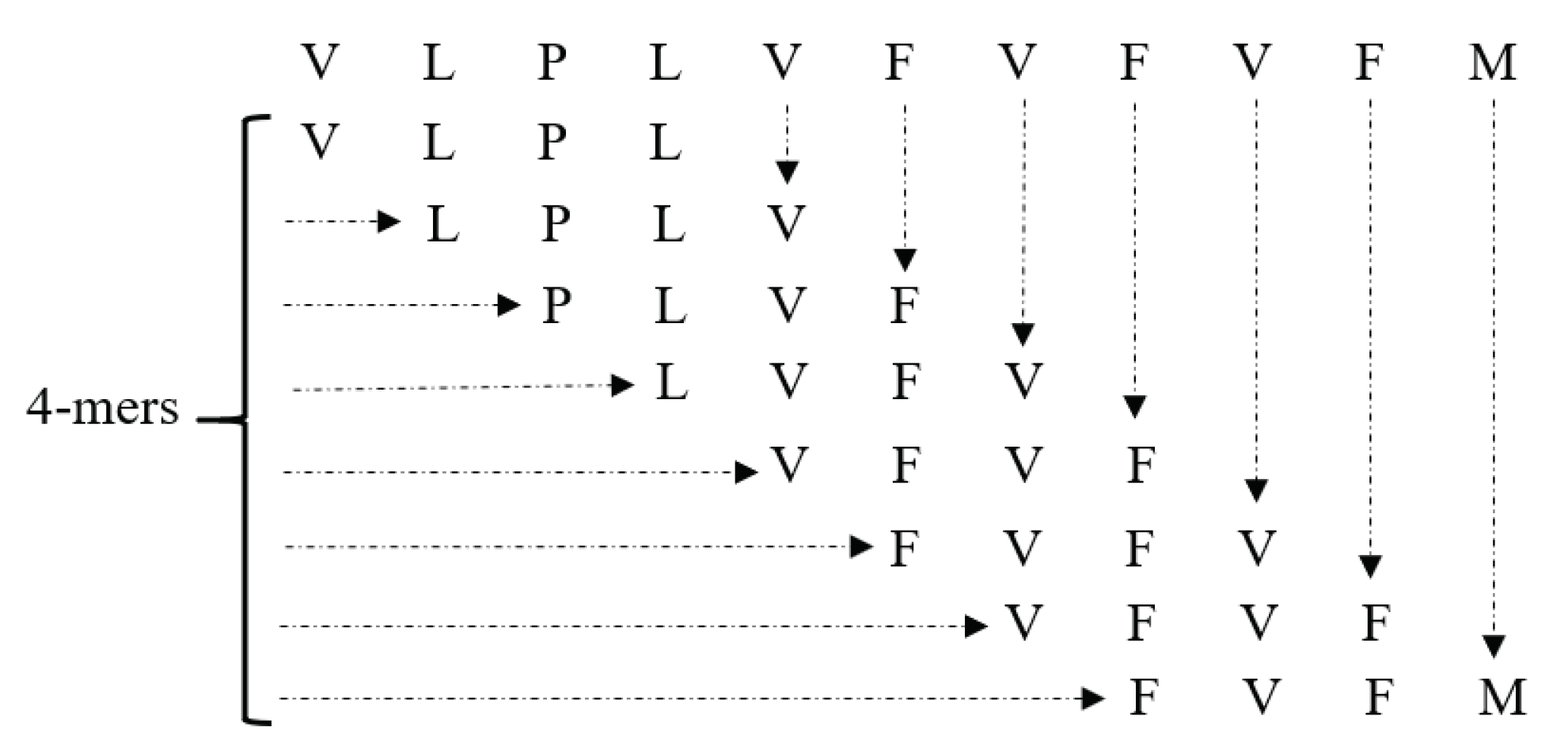
To make use of machine learning approaches, we need to prepare the appropriate input—numerical (real-valued) vectors—that is compatible with these methods. This would give us the ability to perform meaningful analytics. As a result, these amino acid sequences should be converted into numeric characters in a way that preserves some sequential order information of the amino acids within each sequence. The most prevalent strategy in this area is one-hot encoding due to its simplicity [10]. Since we need to compute pairwise distances (e.g., Euclidean distance), one-hot encoding order preservation would not be operational [20]. To preserve order information of each sequence while being amenable to pairwise distance computation, k-mers (length k substrings of each sequence) are calculated and input to the downstream classification/clustering tasks [20,21] (see Figure 2).

Figure 2. Example of 4-mers of the amino acid sequence “VLPLVFVFVFM”.

In this work, we propose a robust feature-vector representation of biological sequences based on k-mers that, when combined with the appropriate feature selection, allows many different downstream clustering approaches to perform well on a variety different measures. This results in fast and efficient clustering methods to cluster the spike amino acid sequences of SARS-CoV-2. We demonstrate that our method performs considerably better than the baseline approach (called one-hot embedding), and the variants are clustered into unique clusters with high $F_1$ score as a result, among other quality metrics. The following are the contributions of this paper:

• For efficient sequence clustering, we propose an embedding based on k-mers, and show that the downstream clustering methods cluster the variants with a high $F_1$ score, among other quality metrics.
• We performed experiments using different clustering algorithms and feature selection approaches and show the trade-off between the clustering quality and the runtime for these methods.
• We use both hard and soft clustering approaches to study the behavior of different coronavirus variants in detail.
• After comparison of our k-mers based algorithm with the baseline embedding method called one-hot embedding (OHE), we show that our proposed model is able to cluster the variants with higher clustering quality.

The rest of the paper is organized as follows: Section 2 contains related work of our approach. Our proposed approach is detailed in Section 3. A description of the datasets used are given in Section 4. We provide a detailed discussion about the results in Section 5, and then we conclude our paper in Section 6.

2. Literature Review

Performing different data analytics tasks on sequences has been done successfully by different researchers previously [20,22]. However, most studies require the sequences to be aligned [10,23,24]. The aligned sequences are used to generate fixed length numerical embeddings, which can then be used for tasks such as classification and clustering [20,25,26]. Since the dimensionality of data are another problem while dealing with larger sized sequences, using approximate methods to compute the similarity between two sequences is a popular approach [21,27,28]. The fixed-length numerical embedding methods have been successfully used in literature for other applications such as predicting missing values in graphs [29], text analytics [30,31,32], biology [21,27,33], graph analytics [34,35], classification of electroencephalography and electromyography sequences [36,37], detecting security attacks in networks [38], and electricity consumption in smart grids [39]. The conditional dependencies between variables is also important to study so that their importance can be analyzed in detail [40].

Due to the availability of large-scale sequence data for the SARS-CoV-2 virus, an accurate and effective clustering method is needed to further analyze this disease, so as to better understand the dynamics and diversity of this virus. To classify different coronavirus hosts, authors in [10] suggest a one-hot encoding-based method that uses spike sequences alone. Their study reveals that they achieved excellent prediction accuracy considering just the spike portion of the genome sequence instead of using the entire sequence. Using this idea and a kernel method, Ali et al. in [20] accomplish higher accuracy than in [10], in the classification of different variants of SARS-CoV-2 in humans. Successful analysis of different variants leads to designing efficient strategy regarding the vaccination distribution [41,42,43,44].

3. Proposed Approach

In this section, we discuss our proposed approach in detail. We start with the description of one-hot embedding (OHE) and k-mers generation from the spike sequences. We then describe how we generated the feature vector representation from the k-mers information. After that, we discuss different feature selection methods in detail. Finally, we detail how we applied clustering approaches on the final feature vector representation.

3.1. One-Hot Embedding Generation

The one-hot embedding [45] is an orthogonal encoding. These embedding arrangements regularly assume there is no prior knowledge about domain information of amino acids. Given a sequence of amino acids “VLPLVFVFVFM”, to convert the sequence to a feature vector representation, we generate binary vectors proportional to the number of amino acids in the sequence. Each of these binary vectors includes 1 when any of the amino acids appear, otherwise 0. In addition, a final feature vector representation would be the concatenation of these vectors.

3.2. k-mers Generation

Given a spike sequence, the first step is to compute all possible k-mers. The total number of k-mers that we can generate for a spike sequence is described as follows:

$$N-k+1,$$

(1)

where N is the length of the spike sequence ($N=1274$ for our dataset). The variable k is a user-defined parameter (we took $k=3$ using standard validation set approach [46]). For an example of how to generate k-mers, see Figure 2.

3.3. Fixed-Length Feature Vector Generation

Since most of the machine learning (ML) models work with a fixed-length feature vector representation, we need to convert the k-mers information into such vectors. For this purpose, we generate a feature vector ${\mathsf{\Phi }}_k$ for a given spike sequence a (i.e., ${\mathsf{\Phi }}_k\left(a\right)$). Given an alphabet $\mathsf{\Sigma }$ (characters representing amino acids in the spike sequence), the length of ${\mathsf{\Phi }}_k\left(a\right)$ will be equal to the number of possible k-mers of a. More formally,

$${\mathsf{\Phi }}_k\left(a\right)={\left|\mathsf{\Sigma }\right|}^k.$$

(2)

Since we have 21 unique characters in $\mathsf{\Sigma }$ (namely ACDEFGHIKLMNPQRSTVWXY), the length of each frequency vector is ${21}^3=9261$.

3.4. Low Dimensional Representation

Since the dimensionality of the data is high after obtaining the fixed length feature vector representation, we apply different supervised and unsupervised methods to obtain a low dimensional representation of data to avoid the problem of the curse of dimensionality [39,47]. Each of the methods for obtaining a low dimensional representation of data is discussed below.

3.4.1. Random Fourier Features

The first method that we use is an approximate kernel method called random Fourier features (RFF) [48]. It is an unsupervised approach, which maps the input data to a randomized low dimensional feature space (Euclidean inner product space) to get an approximate representation of data in lower dimensions D from the original dimensions d. More formally:

$$z:{\mathcal{R}}^d\to {\mathcal{R}}^D.$$

(3)

In this way, we approximate the inner product between a pair of transformed points. More formally:

$$f(x,y)=⟨\varphi \left(x\right),\varphi \left(y\right)⟩\approx z{\left(x\right)}^{\prime }z\left(y\right).$$

(4)

In Equation (4), z is low dimensional (unlike the lifting $\varphi$). Now, z acts as the approximate low dimensional embedding for the original data. We can use z as an input for different ML tasks like clustering and classification.

3.4.2. Least Absolute Shrinkage and Selection Operator (LASSO) Regression

LASSO regression is a supervised method that can be used for efficient feature selection. It is a type of regularized linear regression variant. It is a specific case of the penalized least squares regression with an $L_1$ penalty function. By combining the good qualities of ridge regression [49,50] and subset selection, LASSO can improve both model interpretability, and prediction accuracy [51]. LASSO regression tries to minimize the following objective function:

$$min(\mathrm{Sum}\mathrm{of}\mathrm{square}\mathrm{residuals}+\alpha \times |\mathrm{slope}\left|\right),$$

(5)

where $\alpha \times \left|\mathrm{slope}\right|$ is the penalty term. In LASSO regression, we take the absolute value of the slope in the penalty term rather than the square (as in ridge regression [50]). This helps to reduce the slope of useless variables exactly equal to zero.

3.4.3. Boruta

The last feature selection method that we are using is Boruta. It is a supervised method that is made around the random forest (RF) classification algorithm. It works by creating shadow features so that the features do not compete among themselves, but rather they compete with a randomized version of them [52]. It captures the nonlinear relationships and interactions using the RF algorithm. It then extracts the importance of each feature (corresponding to the class label) and only keeps the features that are above a specific threshold of importance. The threshold is defined as the highest feature importance recorded among the shadow features.

3.5. Clustering Methods

In this paper, we use five different clustering methods (both hard and soft clustering approaches) namely k-means [53], k-modes [54], fuzzy c-means [55,56], agglomerative hierarchical clustering, and hierarchical density-based spatial clustering of applications with noise (HDBSCAN) [57,58] (note that this is a soft clustering approach). For the k-means and k-modes, default parameters are used. For the fuzzy c-means, the clustering criterion used to aggregate subsets is a generalized least-squares objective function. For agglomerative hierarchical clustering, a bottom-up approach is applied, which is acknowledged as the agglomerative method. Since the bottom-up procedure starts from anywhere in the central point of the hierarchy and the lower part of the hierarchy is developed by a less expensive method such as partitional clustering, it can reduce the computational cost [59].

HDBSCAN is not just density-based spatial clustering of applications with noise (DBSCAN) but switches it into a hierarchical clustering algorithm and then obtains a flat clustering based in the solidity of clusters. HDBSCAN is robust to parameter choice and can discover clusters of differing densities (unlike DBSCAN) [58].

3.6. Optimal Number of Clusters

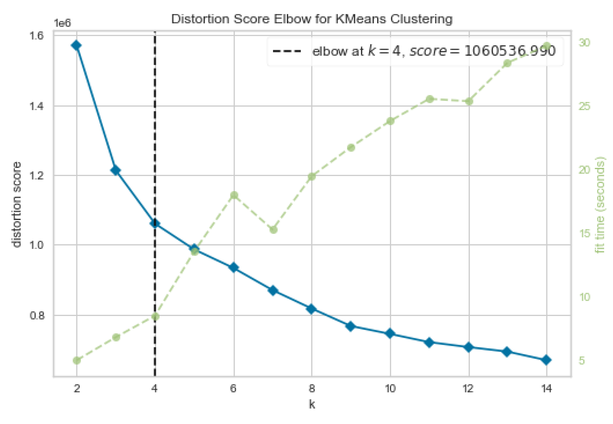
We determined the optimal number of clusters using the elbow method [60]. It can fit the model with a number of clusters k ranging from 2 to 14. As a quality measure, “distortion” is used, which measures the sum of squared distances from each point to its center. Figure 3 shows the distortion score for several values of k. We also plot the training runtime (in seconds) to see the trade-off between the distortion score and the runtime. We use the knee point detection algorithm (KPDA) [60] to determine the optimal number of clusters. Note that, based on results shown in Figure 3, the perfect number of clusters is 4. However, we choose $k=5$ for all hard clustering approaches because we have five different variants in our data (see Table 1). The KPDA chose 4 as the best initial number of clusters due to the Beta variant not being well-represented in the data (see Table 1). However, to give a fair chance to the Beta variant to form its own cluster, we choose 5 as the number of clusters.

Figure 3. The distortion score (blue line) for different numbers of clusters using k-means. The dashed green line shows the runtime (in s). The dashed black line shows the optimal number of clusters computed using the Elbow method [60].

4. Experimental Setup

In this section, first, we provide information associated with the dataset. Then, with the benefit of the t-distributed stochastic neighbor embedding (t-SNE) [61], we try to reduce dimensions with nonlinear relationships to find any natural hidden clustering in the data. This data analysis step helps us to obtain basic knowledge about different variants. As a baseline, we use k-mers based frequency vectors without applying any feature selection to perform clustering using k-means, k-modes, fuzzy, hierarchical, and density-based spatial (HDBSCAN) algorithms. All experiments are performed on a Core i5 system running the Windows operating system, 32 GB memory, and a 2.4 GHz processor. Implementation of the algorithms is done in Python, and the code is available online (https://github.com/sarwanpasha/COVID_19_Community_Detection_For_Variants/tree/main/Results (accessed on 15 October 2021)). Our pre-processed data are also available online (https://drive.google.com/drive/folders/1-YmIM8ipFpj-glr9hSF3t6VuofrpgWUa?usp=sharing (accessed on 20 November 2021)), which can be used after agreeing to the terms and conditions of GISAID (https://www.gisaid.org/ (accessed on 20 November 2021)). The code of HDBSCAN is taken from [58]. The code for fuzzy c-means is also available online (https://github.com/omadson/fuzzy-c-means (accessed on 20 November 2021)).

4.1. Dataset Statistics

Our dataset is the (aligned) amino acid sequences (spike region only) of the SARS-CoV-2 proteome. The dataset is publicly available on the GISAID website (https://www.gisaid.org/ (accessed on 20 November 2021)), which is the largest known database of SARS-CoV-2 sequences. Table 1 shows more information related to the dataset. There are the five most common variants, namely Alpha, Beta, Delta, Gamma, and Epsilon. The fourth column of Table 1 shows the number of mutations that occurred in a spike protein over the number of total mutations (in the whole genome) for each variant, e.g., for the Alpha variant, there are 17 mutations in the whole genome, and eight of these mutations are in the spike region. In our dataset, we have 62,657 amino acid sequences (after removing missing values).

4.2. Data Visualization

By using the t-SNE approach, we plotted the data to 2D real vectors to find any hidden clustering in the data. Figure 4a shows the t-SNE plot for the GISAID dataset (before applying any feature selection). The goal here is to show how well different variants are forming clusters. Since the colors could change randomly because t-SNE is a non-deterministic algorithm just like k-means, we may not have same color for a given variant every time. Different variants in the scatter plot can be easily visualized. Even though we cannot see clear separate clusters for each of those variants, small clusters are obvious for different variants. This evaluation for such data reveals that using any clustering algorithm directly will give us good results, and some data preprocessing is curtailed for efficiently clustering the variants.

Figure 4. t-SNE plots for the original data and for different feature selection methods applied on the original data.

By visualizing the GISAID dataset using t-SNE, more clear clusters are visible after applying three different feature selection methods. In Figure 4b–d, we apply different feature selection methods, namely Boruta, LASSO, and RFF, respectively. We can observe that the clustering is purer for Boruta and LASSO regression but not for RFF. This behavior shows that the supervised methods (LASSO regression and Boruta) are able to preserve the patterns in the data more effectively as compared to the unsupervised RFF. Note that, after feature selection, some data points are still isolated from the big clusters. This behavior shows that, although those isolated data points belong to a certain cluster, they may be potential candidates for developing into a new variant.

4.3. Evaluation Metrics

The goal of validating the quality of clustering methods is the assessment of the similarity of objects in the same cluster and, at the same time, the dissimilarity of objects in different clusters by using a pairwise difference of between- and within-cluster distances [62,63]. We evaluate our models using the following clustering evaluation methods: $F_1$ score (weighted), silhouette coefficient, Calinski–Harabasz index, and Davies–Bouldin index.

4.3.1. $F_1$ Score

The weighted $F_1$ score is used to measure the quality of clustering algorithms for different experimental settings. Since we do not have the ground truth for each cluster, we take the majority variant in each cluster as its class label and compute a weighted $F_1$ score.

4.3.2. Silhouette Coefficient

The silhouette coefficient [64] is used when the model should be evaluated by itself and without any ground truth labels, and a model with well-defined clusters will have a higher silhouette coefficient. The silhouette coefficient is:

$$s=\frac{b-a}{max\{b,a\}},$$

(6)

where a is the average distance between a sample and all other data points in the same class and b is the average distance between a sample and all other data points in the next closest cluster.

4.3.3. Calinski–Harabasz Index

The Calinski–Harabasz index [65] assesses a clustering based on the mean between and inside cluster sum of squares, and a model with better defined clusters will have a higher Calinski–Harabasz index. For a set of data E of size $n_E$ which has been clustered into k clusters, the Calinski–Harabasz index is defined as the ratio of the between-clusters dispersion (the sum of distances squared) mean and the within-clusters dispersion:

$$\frac{tr\left(B_k\right)}{tr\left(W_k\right)}\times \frac{(n_E-k)}{(k-1)},$$

(7)

where $tr\left(B_k\right)$ is the trace of the between cluster dispersion matrix, $tr\left(W_k\right)$ is the trace of the within-group dispersion matrix, E is a set of data, $n_E$ is the size of data, and k is the number of clusters.

4.3.4. Davies–Bouldin Index

The Davies–Bouldin index [66] is another metric to validate models that do not have any ground truth labels. The Davies–Bouldin ($DB$) index of a clustering C is defined as:

$$DB\left(C\right)=\frac{1}{\left|C\right|}\sum _{i=1}^{\left|C\right|}ma{x}_{j\le \left|C\right|,j\ne i}{D}_{ij},$$

(8)

where $D_{ij}$ is the ratio of the “within-to-between cluster distance” of the ith and jth clusters. For each cluster, we essentially compute the worst case ratio ($D_{ij}$) of a within-to-between cluster distance between it and any other cluster, and then take the average. Thus, by minimizing this index, we can make sure that clusters are the most separate from each other. Hence the $DB$ index is smaller when the clustering result is better.

5. Results and Discussion

In this section, we report the results for all clustering approaches without and with feature selection methods. We use the weighted $F_1$ score to assess the performance of clustering. Since we do not have labels available for clusters, we label each cluster using the variant that has most of its sequences in that cluster (e.g., we give the label “Alpha” to that cluster if most of the sequences belong to the Alpha variant). Now, we calculate the $F_1$ score (weighted) for each cluster individually using these given labels. For different methods, the weighted $F_1$ scores are provided in Table 2. Note that we did not mention the $F_1$ scores for HDBSCAN since it is an overlapping clustering approach. From the results, we can observe that LASSO regression is more consistent as compared to Boruta to efficiently cluster all variants. One interesting pattern we can observe is the pure clusters of some variants in the case of RFF. It shows that RFF is able to cluster some variants very efficiently. However, it fails to generalize over all variants. In terms of different clustering methods, k-means and k-modes are performing better and able to generalize more on all variants as compared to the other clustering methods.

Table 2. Variant-wise $F_1$ (weighted) score with mean, standard deviation (S.D.), and runtime for different clustering methods with number of clusters $=5$. Best values are shown in bold.

Embed.	Algorithm	${\mathit{F}}_1$ Score (Weighted) for Different Variants							Runtime (s)
		Alpha	Beta	Delta	Gamma	Epsilon	Mean	S.D.
OHE	k-means	0.36	0.05	0.70	0.46	0.68	0.45	0.27	553.95
	k-means + Boruta	0.62	0.05	0.84	0.98	0.69	0.64	0.36	20.01
	k-means + LASSO	0.50	0.05	0.70	0.69	0.68	0.52	0.28	61.78
	k-means + RFF	0.98	0.0	0.29	0.99	0.99	0.65	0.47	28.02
	k-modes	0.98	0.01	0.99	0.98	0.90	0.77	0.43	198,926.91
	k-modes + Boruta	0.99	0.01	0.80	0.98	0.77	0.71	0.40	6646.35
	k-modes + LASSO	0.98	0.05	0.56	0.98	0.75	0.66	0.39	36,435.04
	k-modes + RFF	0.99	0.0	0.23	0.99	0.99	0.64	0.49	1370.85
	Fuzzy	0.96	0.01	0.68	0.98	0.80	0.69	0.40	29,193.81
	Fuzzy + Boruta	0.60	0.26	0.61	0.98	0.68	0.63	0.26	664.19
	Fuzzy + LASSO	0.96	0.01	0.74	0.98	0.80	0.70	0.40	3958.60
	Fuzzy + RFF	0.44	0.0	0.0	1.00	1.00	0.49	0.50	395.95
	Hierarchical	0.55	0.04	0.69	0.70	0.68	0.53	0.28	106,092.34
	Hierarchical + Boruta	0.59	0.25	0.60	0.99	0.67	0.62	0.26	2761.91
	Hierarchical + LASSO	0.55	0.04	0.19	0.70	0.56	0.41	0.28	8650.66
	Hierarchical + RFF	0.98	0.00	0.29	0.98	0.98	0.65	0.47	2542.87
k-mers	k-means	0.4	0.15	0.61	0.69	0.44	0.45	0.21	66.43
	k-means + Boruta	0.42	0.10	0.61	0.69	0.65	0.50	0.24	15.77
	k-means + LASSO	0.99	0.007	0.84	0.99	0.77	0.72	0.41	9.56
	k-means + RFF	1.00	0.0	0.28	1.00	1.00	0.66	0.48	8.65
	k-modes	0.99	0.005	0.87	0.99	0.77	0.73	0.42	17,580.25
	k-modes + Boruta	0.99	0.31	0.86	0.99	0.85	0.81	0.28	2965.03
	k-modes + LASSO	0.99	0.17	0.99	0.99	0.07	0.63	0.47	784.20
	k-modes + RFF	1.00	0.00	0.0	0.61	1.00	0.52	0.50	794.56
	Fuzzy	0.35	0.10	0.61	0.69	0.44	0.44	0.23	2358.84
	Fuzzy + Boruta	0.36	0.15	0.61	0.69	0.44	0.45	0.21	230.17
	Fuzzy + LASSO	0.99	0.31	0.65	0.99	0.82	0.76	0.29	94.36
	Fuzzy + RFF	0.44	0.0	0.0	1.00	0.0	0.29	0.44	460.82
	Hierarchical	0.32	0.10	0.58	0.70	0.46	0.43	0.23	9934.57
	Hierarchical + Boruta	0.36	0.14	0.63	0.68	0.46	0.45	0.22	1908.75
	Hierarchical + LASSO	0.99	0.58	0.58	0.99	0.83	0.80	0.21	713.07
	Hierarchical + RFF	1.00	0.00	0.28	1.00	1.00	0.66	0.48	1120.14

In addition, the results of other clustering validation metrics of Table 3 (silhouette coefficient, Calinski–Harabasz index, and Davies–Bouldin index) signify that for k-mers feature vectors and without using any feature selection methods, the fuzzy clustering method has acceptable results, which is a high silhouette coefficient score, high Calinski–Harabasz index and low Davies–Bouldin index, but higher running time (bold rows in Table 3). Interestingly, using k-mers and applying the fuzzy clustering method with the Boruta feature selection method give even better results in terms of the three different metrics and running time. Other acceptable performances that validate the effectiveness of using k-mers and feature selection methods regarding clustering quality and running time are related to the combination of k-means clustering and LASSO feature selection method and fuzzy clustering and RFF feature selection method. In addition, we can see that there is a trade-off between the quality of clustering and runtime between k-means and Fuzzy clustering methods. Moreover, comparing the results of using k-mers with the results of using one-hot embedding feature vectors shows that k-means and LASSO feature selection method has a high silhouette coefficient, high Calinski–Harabasz index score and low Davies–Bouldin index, and the lowest runtime. However, in general, the improvement in quality of clustering and runtimes are observable when we compare using one-hot encoding and k-mers, the same metrics for k-means clustering and the LASSO feature selection method, and other different clustering methods given in Table 3.

Table 3. Clustering quality metrics for different clustering methods with number of clusters $=5$. Best values are shown in bold.

Embedding	Algorithm	Different Metrics for Different Variants			Runtime (s)
		Silhouette Coefficient	Calinski–Harabasz Index	Davies–Bouldin Index
OHE	k-means	0.48	13,089.36	1.38	553.95
	k-means + Boruta	0.34	17,478.82	1.4	20.01
	k-means + LASSO	0.48	13,112.61	1.38	61.78
	k-means + RFF	0.25	4855.80	2.04	28.02
	k-modes	0.26	6626.82	2.59	198,926.91
	k-modes + Boruta	0.33	13,146.09	1.89	6646.35
	k-modes + LASSO	0.28	9596.01	1.92	36,435.04
	k-modes + RFF	$-0.15$	1389.75	1.07	1370.85
	Fuzzy	0.27	8821.95	2.13	29,193.81
	Fuzzy + Boruta	0.33	13,397.80	1.89	664.19
	Fuzzy + LASSO	0.26	8663.69	2.17	3958.60
	Fuzzy + RFF	0.19	12,069.50	1.09	395.95
	Hierarchical	0.44	10,516.02	1.84	106,092.34
	Hierarchical + Boruta	0.32	13,324.79	1.60	2761.91
	Hierarchical + LASSO	0.42	10,529.10	1.61	8650.66
	Hierarchical + RFF	0.26	5010.25	1.00	2542.87
k-mers	k-means	0.75	329,866.74	0.45	66.43
	k-means + Boruta	0.76	342,083.63	0.43	15.77
	k-means + LASSO	0.42	17,269.34	1.52	9.56
	k-means + RFF	0.25	5251.93	1.55	8.65
	k-modes	0.05	10,257.1	7.11	17,580.25
	k-modes + Boruta	0.07	12,058.15	6.52	2965.03
	k-modes + LASSO	0.42	15,704.43	1.54	784.20
	k-modes + RFF	$-0.15$	13,66.91	1.07	794.56
	Fuzzy	0.75	329,410.74	0.44	2358.84
	Fuzzy + Boruta	0.76	341,678.01	0.43	230.17
	Fuzzy + LASSO	0.41	15,010.79	2.58	94.36
	Fuzzy + RFF	0.19	13,293.96	0.99	460.82
	Hierarchical	0.72	284,726.92	0.47	9934.57
	Hierarchical + Boruta	0.73	280,129.56	0.42	1908.75
	Hierarchical + LASSO	0.41	15,218.95	2.03	713.07
	Hierarchical + RFF	0.26	5258.43	1.00	1120.14

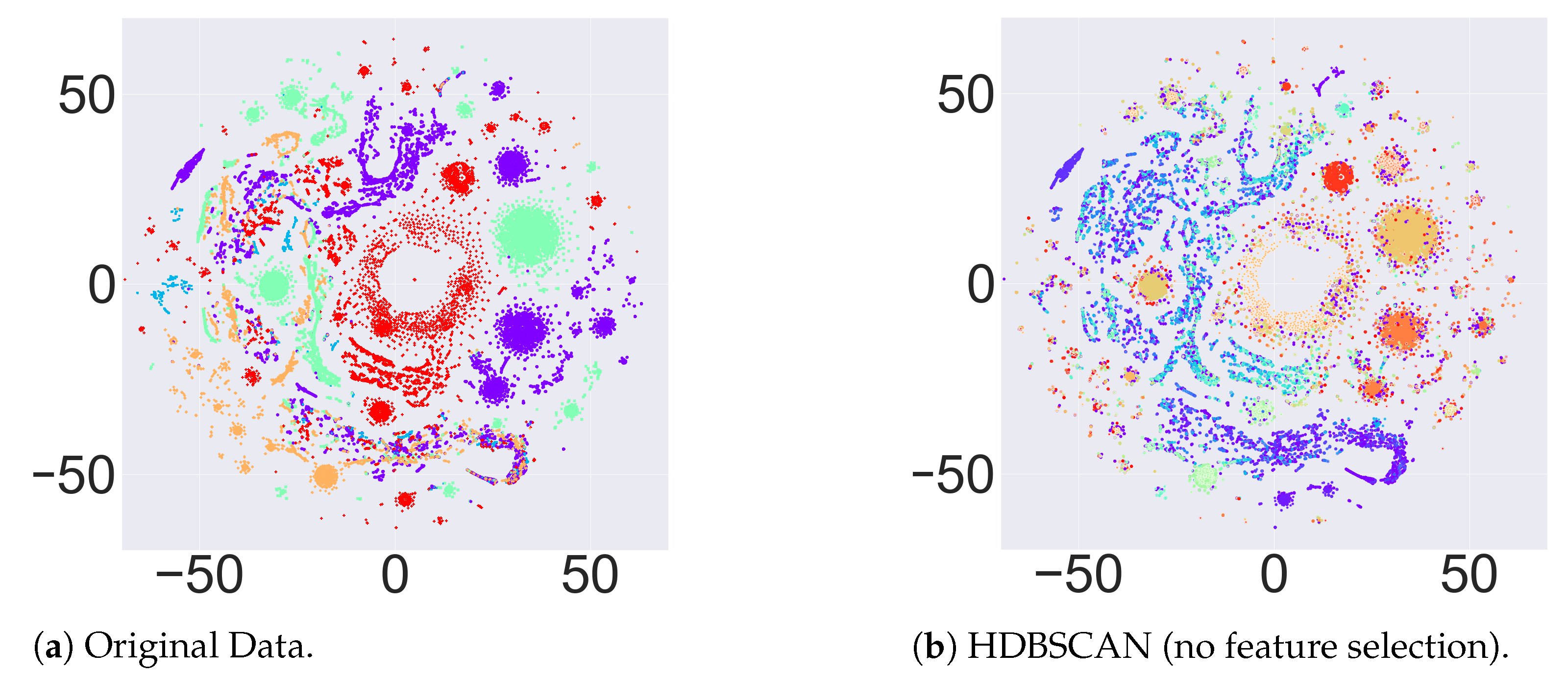
In terms of studying the behavior of different known variants, we are interested to see if there is any similarity between variants, that is, if two different variants can form a single cluster. Since we can observe from Table 2 that almost all variants apart from the Beta variant form separate clusters (for some experimental settings), it is evident that these variants are not directly related to each other. From this analysis, we can conclude that, for example, designing a single vaccination for all variants may not be appropriate. Another point was to see if a single variant could make more than one cluster. The idea of this analysis was to observe if a new variant could be developed from an existing variant. For this purpose, we used the soft clustering approach HDBSCAN. We can observe in Figure 5 and Figure 6 that there are certain small clusters appearing in the data. They may be potential candidates for a developing new coronavirus variant.

Figure 5. (a) t-SNE plots for the original variants as labels; (b) t-SNE plot with labels obtained after applying HDBSCAN without any feature selection method on the frequency vectors.

Figure 6. t-SNE plots for HDBSCAN without and with feature selection methods.

5.1. Contingency Tables

After evaluating the clustering methods using different metrics, we compute the contingency tables for variants versus clusters for different clustering approaches. The contingency tables for different clustering methods and feature selection approaches (using k-mers and one-hot embedding) are given in Table 4, Table 5, Table 6, Table 7, Table 8, Table 9, Table 10, Table 11, Table 12, Table 13, Table 14, Table 15, Table 16, Table 17, Table 18 and Table 19. In Table 4, we can observe that k-modes without applying any feature selection is outperforming k-means and also the other two clustering algorithms from Table 6. In Table 8 and Table 10, we can observe that RFF is giving pure clusters for some of the variants but performing poorly on the other variants. For LASSO regression in Table 12 and Table 14, we can observe that clusters started to become pure immediately when we apply LASSO regression. This shows the effectiveness of this feature selection method for the clustering of spike sequences. Similarly, in Table 16 and Table 18, we can see that Boruta is not giving many pure clusters (apart from k-modes). This shows that Boruta fails to generalize over different clustering approaches and different variants. Comparing these results of contingency tables for k-mers with the results of one-hot embedding, improvement of k-mers results are obvious in terms of purity of clustering. In addition, we can see that, even with using one-hot embedding, using the feature selection methods improves the clustering purity. In addition, in Table 5 and Table 7, without using any feature selection methods, we can see that k-modes is outperforming the other clustering algorithms. In Table 9 and Table 11, clear clusters as a result of clustering methods and RFF can prove the effectiveness of this feature selection method. The results of applying different clustering algorithms and using LASSO feature selection method in Table 13 and Table 15 also show the enhancements in terms of clustering quality, but, compared to RFF, it is not significant. The same pattern is observable in Table 17 and Table 19, which are the results of using the Boruta feature selection method, showing weakness in generalization over different clustering approaches and different variants.

Table 4. Contingency tables of variants vs. clusters (no feature selection, k-mers) with number of clusters $=5$.

Variant	k-means (Cluster IDs)					k-modes (Cluster IDs)
	0	1	2	3	4	0	1	2	3	4
Alpha	1512	8762	2926	680	86	8	11,492	284	330	1852
Beta	295	601	626	172	33	64	9	1604	31	19
Epsilon	956	7848	3155	638	187	0	1	8532	613	3638
Delta	2706	2605	1342	868	30	0	1	3192	3491	867
Gamma	682	22,140	3016	741	50	26,519	7	7	61	35

Table 5. Contingency tables of variants vs. clusters (no feature selection, one-hot embedding) with number of clusters $=5$.

Variant	k-means (Cluster IDs)					k-modes (Cluster IDs)
	0	1	2	3	4	0	1	2	3	4
Alpha	52	9716	1601	2165	432	11,235	13	2316	25	377
Beta	24	650	1011	18	24	5	81	30	29	1582
Epsilon	427	7972	223	3626	536	8	0	4111	18	8647
Delta	5	2800	484	1201	3061	3	0	3988	3490	70
Gamma	513	23,032	1425	70	1589	6	26,502	114	0	7

Table 6. Contingency tables of variants vs. clusters (no feature selection, k-mers) with number of clusters $=5$.

Variant	Fuzzy (Cluster IDs)					Hierarchical (Cluster IDs)
	0	1	2	3	4	0	1	2	3	4
Alpha	666	1515	78	2945	8762	1772	3442	650	8036	66
Beta	171	279	31	627	601	501	491	164	544	27
Epsilon	637	942	186	3172	7847	1166	3804	636	6994	184
Delta	839	2725	28	1354	2605	2997	1292	827	2411	24
Gamma	739	669	47	3034	22,140	865	3501	734	21,484	45

Table 7. Contingency tables of variants vs. clusters (no feature selection, one-hot embedding) with number of clusters $=5$.

Variant	Fuzzy (Cluster IDs)					Hierarchical (Cluster IDs)
	0	1	2	3	4	0	1	2	3	4
Alpha	629	11,005	2101	226	5	2845	8651	32	244	2194
Beta	213	508	19	987	0	1002	605	18	35	67
Epsilon	713	16	3597	8458	0	520	7324	426	457	4057
Delta	3419	74	1042	3016	0	1168	2547	2	2479	1355
Gamma	1590	262	88	61	24,628	2008	22,333	497	1522	269

Table 8. Contingency tables of variants vs. clusters (random Fourier feature selection, k-mers) with number of clusters $=5$.

Variant	k-means (Cluster IDs)					k-modes (Cluster IDs)
	0	1	2	3	4	0	1	2	3	4
Alpha	0	12,603	0	1363	0	12,603	0	0	1363	0
Beta	0	1727	0	0	0	1727	0	0	0	0
Epsilon	0	10,348	0	0	2436	10,348	0	2436	0	0
Delta	0	7551	0	0	0	7551	0	0	0	0
Gamma	13,076	12,569	984	0	0	25,632	13	0	0	984

Table 9. Contingency tables of variants vs. clusters (random Fourier feature selection, one-hot embedding) with number of clusters $=5$.

Variant	k-means (Cluster IDs)					k-modes (Cluster IDs)
	0	1	2	3	4	0	1	2	3	4
Alpha	0	0	0	1363	12,603	12,603	0	0	0	1363
Beta	0	0	0	0	1727	1727	0	0	0	0
Epsilon	0	2436	0	0	10,348	10,348	0	2436	0	0
Delta	0	0	637	0	6914	7551	0	0	0	0
Gamma	13,076	0	984	0	12,569	25,632	13	0	984	0

Table 10. Contingency tables of variants vs. clusters (random Fourier feature selection, k-mers) with number of clusters $=5$.

Variant	Fuzzy (Cluster IDs)					Hierarchical (Cluster IDs)
	0	1	2	3	4	0	1	2	3	4
Alpha	0	0	0	13,966	0	12,603	0	0	1363	0
Beta	0	0	0	1727	0	1727	0	0	0	0
Epsilon	0	0	0	12,784	0	10,348	0	2436	0	0
Delta	0	0	0	7551	0	7551	0	0	0	0
Gamma	0	0	0	13,553	13,076	12,569	13,076	0	0	984

Table 11. Contingency tables of variants vs. clusters (random Fourier feature selection, one-hot embedding) with number of clusters $=5$.

Variant	Fuzzy (Cluster IDs)					Hierarchical (Cluster IDs)
	0	1	2	3	4	0	1	2	3	4
Alpha	0	0	0	13,966	0	12,603	0	0	1363	0
Beta	0	0	0	1727	0	1727	0	0	0	0
Epsilon	0	0	0	12,784	0	10,348	0	2436	0	0
Delta	0	0	0	7551	0	7551	0	0	0	0
Gamma	0	0	0	13,269	13,360	12,569	13,076	0	0	984

Table 12. Contingency tables of variants vs. clusters (LASSO feature selection, k-mers) with number of clusters $=5$.

Variant	k-means (Cluster IDs)					k-modes (Cluster IDs)
	0	1	2	3	4	0	1	2	3	4
Alpha	303	11,365	383	1909	6	8	10,958	282	2660	58
Beta	1551	4	148	23	1	65	9	1617	12	24
Epsilon	8536	1	671	3576	0	0	1	12,000	112	671
Delta	3098	0	3693	760	0	0	0	3121	19	4411
Gamma	16	13	198	36	26,366	26,577	7	7	0	38

Table 13. Contingency tables of variants vs. clusters (LASSO feature selection, one-hot embedding) with number of clusters $=5$.

Variant	k-means (Cluster IDs)					k-modes (Cluster IDs)
	0	1	2	3	4	0	1	2	3	4
Alpha	53	9716	431	2165	1601	11,208	2295	13	63	387
Beta	24	650	24	18	1011	3	28	76	28	1592
Epsilon	427	7972	536	3626	223	4	3981	0	427	8372
Delta	41	4015	0	9	34,864	41	4015	0	9	3486
Gamma	514	23,031	1586	70	1428	5	114	25,989	514	7

Table 14. Contingency tables of variants vs. clusters (LASSO feature selection, k-mers) with number of clusters $=5$.

Variant	Fuzzy (Cluster IDs)					Hierarchical (Cluster IDs)
	0	1	2	3	4	0	1	2	3	4
Alpha	1344	5	12,042	362	213	1967	606	30	11,345	18
Beta	99	1	6	440	1181	24	1667	6	22	8
Epsilon	3220	0	0	780	8784	3667	509	8582	26	0
Delta	4464	0	0	543	2544	3892	245	3367	40	7
Gamma	202	26,169	16	232	10	12	1053	1	11	25,552

Table 15. Contingency tables of variants vs. clusters (LASSO feature selection, one-hot embedding) with number of clusters $=5$.

Variant	Fuzzy (Cluster IDs)					Hierarchical (Cluster IDs)
	0	1	2	3	4	0	1	2	3	4
Alpha	2079	11,051	604	227	5	2671	8521	32	2635	107
Beta	19	476	214	1018	0	92	566	18	1031	20
Epsilon	3525	15	712	8532	0	4650	7218	426	457	33
Delta	1040	70	3385	3056	0	4189	2473	2	690	197
Gamma	87	251	799	75	25,417	352	22,158	497	2155	1467

Table 16. Contingency tables of variants vs. clusters (Boruta feature selection, k-mers) with number of clusters $=5$.

Variant	k-means (Cluster IDs)					k-modes (Cluster IDs)
	0	1	2	3	4	0	1	2	3	4
Alpha	8762	86	2925	680	1513	11,403	7	184	1823	549
Beta	601	33	626	172	295	6	6	640	1060	15
Epsilon	7848	187	3155	638	956	1	0	11,170	947	666
Delta	2605	30	1342	868	2706	0	0	2894	690	3967
Gamma	22,140	50	3016	741	682	6	25,428	6	1128	61

Table 17. Contingency tables of variants vs. clusters (Boruta feature selection, one-hot embedding) with number of clusters $=5$.

Variant	k-means (Cluster IDs)					k-modes (Cluster IDs)
	0	1	2	3	4	0	1	2	3	4
Alpha	10	368	1586	9901	2101	1829	7	552	188	11,390
Beta	22	12	1022	652	19	1060	6	15	640	6
Epsilon	5	624	218	8351	3586	951	0	671	11,161	1
Delta	0	3073	476	2988	1014	695	0	3970	2886	0
Gamma	25,015	95	1417	34	68	1131	25,425	61	6	6

Table 18. Contingency tables of variants vs. clusters (Boruta feature selection, k-mers) with number of clusters $=5$.

Variant	Fuzzy (Cluster IDs)					Hierarchical (Cluster IDs)
	0	1	2	3	4	0	1	2	3	4
Alpha	668	1513	78	2945	8762	9373	702	2641	1198	52
Beta	171	297	31	627	601	823	170	457	254	23
Epsilon	637	943	186	3170	7848	8419	644	2949	591	181
Delta	851	2713	28	1354	2605	2847	879	1563	2245	17
Gamma	739	669	47	3034	22,140	22,955	743	2330	560	41

Table 19. Contingency tables of variants vs. clusters (Boruta feature selection, one-hot embedding) with number of clusters $=5$.

Variant	Fuzzy (Cluster IDs)					Hierarchical (Cluster IDs)
	0	1	2	3	4	0	1	2	3	4
Alpha	2172	11,083	438	268	5	1977	1585	543	9839	22
Beta	26	46	103	1552	0	898	7	198	623	1
Epsilon	3682	4	656	8442	0	546	2983	641	8613	1
Delta	1049	37	3269	3196	0	949	1235	2635	2731	1
Gamma	96	29	389	139	25,976	1703	26	2017	1192	21,691

5.2. HDBSCAN Clustering

After doing an analysis on hard clustering algorithms, we evaluate the performance of the soft clustering approach (HDBSCAN) in this section. To evaluate HDBSCAN, we use the t-SNE approach to plot the original variants from our data and compare them with clusters we obtained after applying HDBSCAN. Since this is a soft clustering approach (overlapping allowed), there were a large number of clusters inferred for different feature selection methods (see Table 20 for the number of clusters). Therefore, we use t-SNE to plot the clusters to visually observe the patterns before and after clustering. Figure 5 shows the comparison of the t-SNE plot on the original data versus t-SNE plots for the clustering results after applying HDBSCAN. Since overlapping is allowed in this setting, we cannot see any pure clusters as compared to the original t-SNE plot. An interesting finding from such a result is that not all sequences corresponding to a specific variant are similar. This means that a small cluster of sequences that initially belong to a certain variant can make another subgroup, which could eventually lead to the developing of a new variant. Therefore, using such overlapping clustering approach, we can visually observe if a group of sequences is diverging from its parent variant. Biologists and other decision-making authorities can then take relevant measures to deal with such scenarios. The t-SNE plots for different feature selection methods are given in Figure 6.

Table 20. Number of clusters for HDBSCAN clustering with different feature selection methods.

Algorithm	Number of Clusters
HDBSCAN	2016
HDBSCAN + Boruta	1419
HDBSCAN + LASSO	1838
HDBSCAN + RFF	1947

5.3. Runtime Comparison

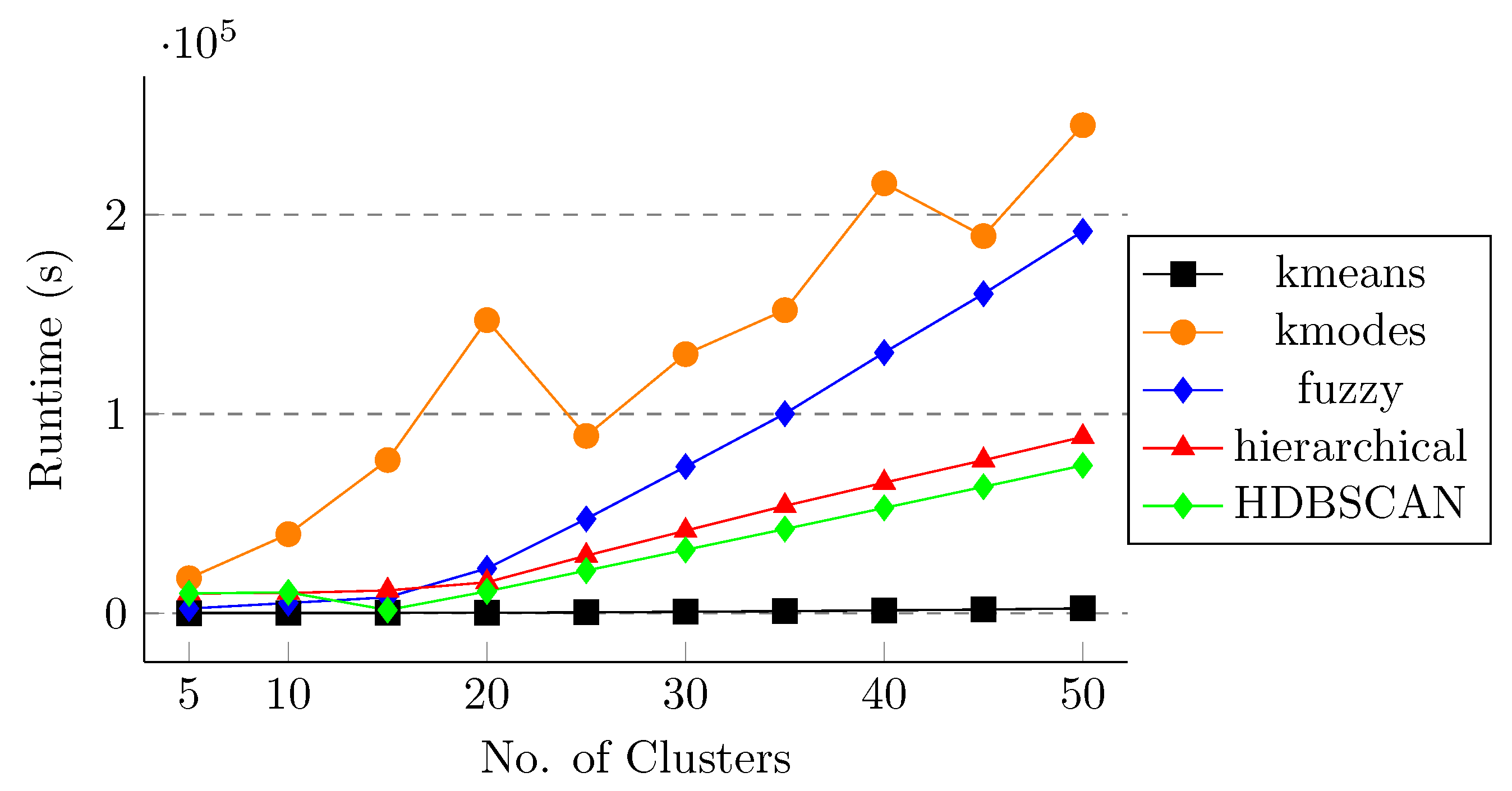
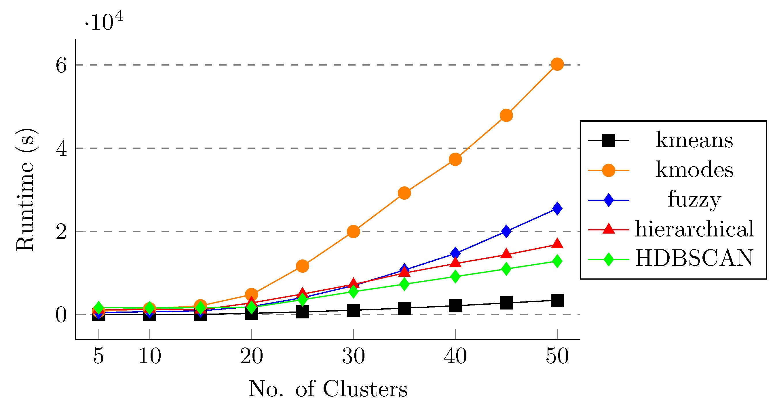
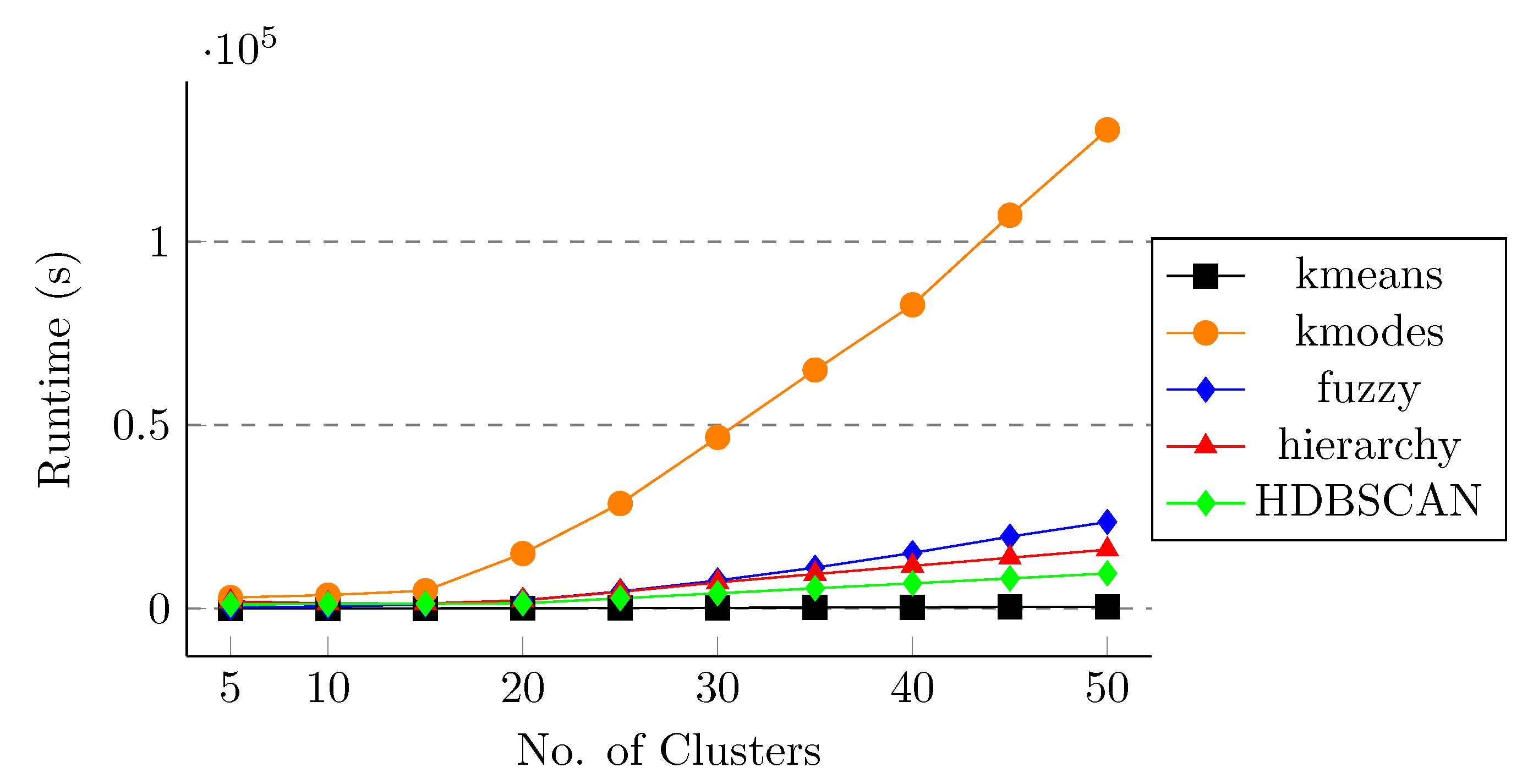
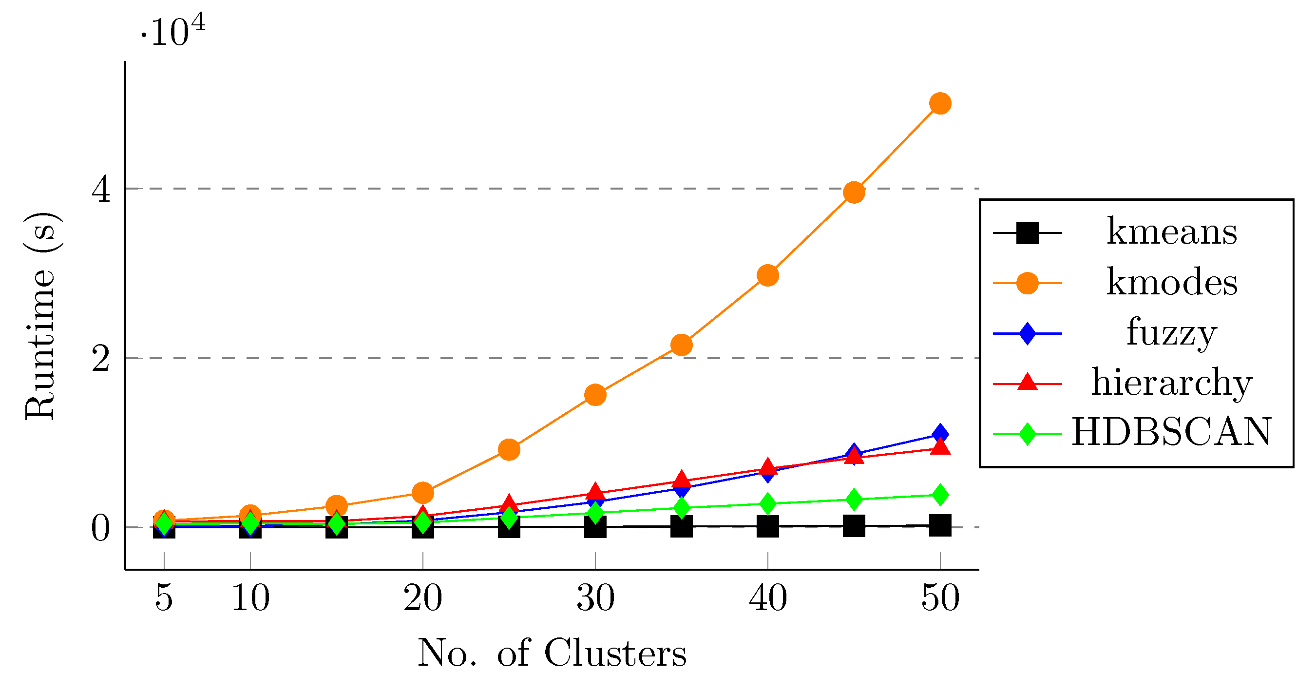
After applying different clustering methods and feature selection algorithms on the spike sequences, we observe that k-means and k-modes are performing better than the other clustering methods in terms of weighted $F_1$ score and k-means and fuzzy in terms of other clustering quality metrics. However, it is also important to study the effect of runtime for these clustering approaches so that we can evaluate the trade-off between the $F_1$ score and the runtime. For this purpose, we compute the runtime of different clustering algorithms for both one-hot embedding and k-mer feature vectors without and with feature selection methods. Figure 7 shows the runtime for all five clustering methods without applying any feature selection on the data. We can observe that applying k-modes is very expensive in terms of runtime and k-means takes the least amount of time to execute. Similar behavior is observed in Figure 8, Figure 9 and Figure 10 for RFF, Boruta, and LASSO regression, respectively. This behavior shows that, although k-modes and fuzzy are performing better in terms of $F_1$ score and clustering quality metrics, k-modes is an outlier in terms of runtime, and fuzzy is more expensive than k-means. This behavior also shows the effectiveness of the k-means algorithm in terms of $F_1$ score, clustering quality metrics, and also in terms of runtime.

Figure 7. Runtime for different clustering methods (no feature selection method). The x-axis shows number of clusters.

Figure 8. Runtime for different clustering methods (random Fourier feature selection). The x-axis shows number of clusters.

Figure 9. Runtime for different clustering methods (Boruta feature selection). The x-axis shows number of clusters.

Figure 10. Runtime for different clustering methods (LASSO feature selection). The x-axis shows number of clusters.

6. Conclusions

We propose a feature vector representation and a set of feature selection methods to eliminate the less important features, allowing many different clustering methods to cluster SARS-CoV-2 spike protein sequences with high $F_1$ scores and other quality metrics. We show that runtime is also an important factor while clustering the coronavirus spike sequences. The k-means algorithm is able to generalize over all variants in terms of clustering purity and also in the least amount of runtime. One possible future work is to use more data for the analysis. Testing out additional clustering methods could be another direction. Additional quality metrics such as clustering entropy is another idea. Using deep learning on even bigger data could give us some interesting insights. Another interesting extension is to compute other feature vector representations, e.g., based on minimizers, which can be done without the need for aligning the sequences. This would allow us to use all of this clustering machinery to study unaligned (even unassembled) sequencing reads of intra-host viral populations to unveil the interesting dynamics at this scale.

References

- World Health Organization. Genomic Sequencing of SARS-CoV-2: A Guide to Implementation for Maximum Impact on Public Health, 8 January 2021; World Health Organization: Geneva, Switzerland, 2021. [Google Scholar]
- Lu, R.; Zhao, X.; Li, J.; Niu, P.; Yang, B.; Wu, H.; Wang, W.; Song, H.; Huang, B.; Zhu, N.; et al. Genomic characterisation and epidemiology of 2019 novel coronavirus: Implications for virus origins and receptor binding. Lancet 2020, 395, 565–574. [Google Scholar] [CrossRef]
- Chen, L.; Liu, W.; Zhang, Q.; Xu, K.; Ye, G.; Wu, W.; Sun, Z.; Liu, F.; Wu, K.; Zhong, B.; et al. RNA based mNGS approach identifies a novel human coronavirus from two individual pneumonia cases in 2019 Wuhan outbreak. Emerg. Microbes Infect. 2020, 9, 313–319. [Google Scholar] [CrossRef]
- Chan, J.F.W.; Kok, K.H.; Zhu, Z.; Chu, H.; To, K.K.W.; Yuan, S.; Yuen, K.Y. Genomic characterization of the 2019 novel human-pathogenic coronavirus isolated from a patient with atypical pneumonia after visiting Wuhan. Emerg. Microbes Infect. 2020, 9, 221–236. [Google Scholar] [CrossRef]
- Weissenhorn, W.; Dessen, A.; Calder, L.; Harrison, S.; Skehel, J.; Wiley, D. Structural basis for membrane fusion by enveloped viruses. Mol. Membr. Biol. 1999, 16, 3–9. [Google Scholar] [CrossRef]
- Walls, A.C.; Park, Y.J.; Tortorici, M.A.; Wall, A.; McGuire, A.T.; Veesler, D. Structure, function, and antigenicity of the SARS-CoV-2 spike glycoprotein. Cell 2020, 181, 281–292. [Google Scholar] [CrossRef]
- Lan, J.; Ge, J.; Yu, J.; Shan, S.; Zhou, H.; Fan, S.; Zhang, Q.; Shi, X.; Wang, Q.; Zhang, L.; et al. Structure of the SARS-CoV-2 spike receptor-binding domain bound to the ACE2 receptor. Nature 2020, 581, 215–220. [Google Scholar] [CrossRef] [PubMed]
- Gui, M.; Song, W.; Zhou, H.; Xu, J.; Chen, S.; Xiang, Y.; Wang, X. Cryo-electron microscopy structures of the SARS-CoV spike glycoprotein reveal a prerequisite conformational state for receptor binding. Cell Res. 2017, 27, 119–129. [Google Scholar] [CrossRef] [PubMed]
- Huang, Y.; Yang, C.; Xu, X.f.; Xu, W.; Liu, S.w. Structural and functional properties of SARS-CoV-2 spike protein: Potential antivirus drug development for COVID-19. Acta Pharmacol. Sin. 2020, 41, 1141–1149. [Google Scholar] [CrossRef] [PubMed]
- Kuzmin, K.; Adeniyi, A.E.; DaSouza, A.K., Jr.; Lim, D.; Nguyen, H.; Molina, N.R.; Xiong, L.; Weber, I.T.; Harrison, R.W. Machine learning methods accurately predict host specificity of coronaviruses based on spike sequences alone. Biochem. Biophys. Res. Commun. 2020, 533, 553–558. [Google Scholar] [CrossRef] [PubMed]
- Harvey, W.T.; Carabelli, A.M.; Jackson, B.; Gupta, R.K.; Thomson, E.C.; Harrison, E.M.; Ludden, C.; Reeve, R.; Rambaut, A.; Peacock, S.J.; et al. SARS-CoV-2 variants, spike mutations and immune escape. Nat. Rev. Microbiol. 2021, 19, 409–424. [Google Scholar] [CrossRef] [PubMed]
- Galloway, S.; Paul, P.; MacCannell, D.R.; Johansson, M.A.; Brooks, J.T.; MacNeil, A.; Slayton, R.B.; Tong, S.; Silk, B.J.; Armstrong, G.L.; et al. Emergence of SARS-CoV-2 b. 1.1. 7 lineage. Morb. Mortal. Wkly. Rep. 2021, 70, 95. [Google Scholar] [CrossRef] [PubMed]
- Yadav, P.; Sapkal, G.N.; Abraham, P.; Deshpande, G.; Nyayanit, D.; Patil, D.Y.; Gupta, N.; Sahay, R.R.; Shete, A.; Kumar, S.; et al. Neutralization potential of Covishield vaccinated individuals sera against B.1.617.1. bioRxiv 2021, 1. [Google Scholar] [CrossRef]
- Naveca, F.; Nascimento, V.; Souza, V.; Corado, A.; Nascimento, F.; Silva, G.; Costa, A.; Duarte, D.; Pessoa, K.; Gonçalves, L.; et al. Phylogenetic Relationship of SARS-CoV-2 Sequences from Amazonas with Emerging Brazilian Variants Harboring Mutations E484K and N501Y in the Spike Protein. Available online: https://virological.org/t/phylogenetic-relationship-of-sars-cov-2-sequences-from-amazonas-with-emerging-brazilian-variants-harboring-mutations-e484k-and-n501y-in-the-spike-protein/585 (accessed on 24 November 2021).
- Zhang, W.; Davis, B.D.; Chen, S.S.; Martinez, J.M.S.; Plummer, J.T.; Vail, E. Emergence of a novel SARS-CoV-2 variant in Southern California. JAMA 2021, 325, 1324–1326. [Google Scholar] [CrossRef]
- Hadfield, J.; Megill, C.; Bell, S.; Huddleston, J.; Potter, B.; Callender, C.; Sagulenko, P.; Bedford, T.; Neher, R. Next, strain: Real-time tracking of pathogen evolution. Bioinformatics 2018, 34, 4121–4123. [Google Scholar] [CrossRef] [PubMed]
- Guyon, I.; Elisseeff, A. An introduction to variable and feature selection. J. Mach. Learn. Res. 2003, 3, 1157–1182. [Google Scholar]
- Ngiam, K.Y.; Khor, W. Big data and machine learning algorithms for health-care delivery. Lancet Oncol. 2019, 20, e262–e273. [Google Scholar] [CrossRef]
- Van Der Maaten, L.; Postma, E.; Van den Herik, J. Dimensionality reduction: A comparative. J. Mach. Learn. Res. 2009, 10, 13. [Google Scholar]
- Ali, S.; Sahoo, B.; Ullah, N.; Zelikovskiy, A.; Patterson, M.D.; Khan, I. A k-mer Based Approach for SARS-CoV-2 Variant Identification. In Proceedings of the International Symposium on Bioinformatics Research and Applications (ISBRA), Shenzhen, China, 26–28 November 2021. [Google Scholar]
- Farhan, M.; Tariq, J.; Zaman, A.; Shabbir, M.; Khan, I. Efficient Approximation Algorithms for Strings Kernel Based Sequence Classification. In Proceedings of the Advances in Neural Information Processing Systems (NeurIPS), Long Beach, CA, USA, 4–9 December 2017; pp. 6935–6945. [Google Scholar]
- Krishnan, G.; Kamath, S.; Sugumaran, V. Predicting Vaccine Hesitancy and Vaccine Sentiment Using Topic Modeling and Evolutionary Optimization. In Proceedings of the International Conference on Applications of Natural Language to Information Systems (NLDB), Saarbrücken, Germany, 23–25 June 2021; pp. 255–263. [Google Scholar]
- Dwivedi, S.K.; Sengupta, S. Classification of HIV-1 Sequences Using Profile Hidden Markov Models. PLoS ONE 2012, 7, e36566. [Google Scholar] [CrossRef][Green Version]
- Melnyk, A.; Mohebbi, F.; Knyazev, S.; Sahoo, B.; Hosseini, R.; Skums, P.; Zelikovsky, A.; Patterson, M. From alpha to zeta: Identifying variants and subtypes of SARS-CoV-2 via clustering. J. Comput. Biol. 2021, 1113–1129. [Google Scholar] [CrossRef]
- Ali, S.; Ali, T.-E.; Khan, M.A.; Khan, I.; Patterson, M. Effective and scalable clustering of SARS-CoV-2 sequences. In Proceedings of the International Conference on Big Data Research (ICBDR), Tokyo, Japan, 25–27 September 2021. [Google Scholar]
- Ali, S.; Patterson, M. Spike2vec: An efficient and scalable embedding approach for covid-19 spike sequences. arXiv 2021, arXiv:2109.05019. [Google Scholar]
- Kuksa, P.; Khan, I.; Pavlovic, V. Generalized Similarity Kernels for Efficient Sequence Classification. In Proceedings of the SIAM International Conference on Data Mining (SDM), Anaheim, CA, USA, 26–28 April 2012; pp. 873–882. [Google Scholar]
- Hoffmann, H. Kernel PCA for novelty detection. Pattern Recognit. 2007, 40, 863–874. [Google Scholar] [CrossRef]
- Ali, S.; Shakeel, M.; Khan, I.; Faizullah, S.; Khan, M. Predicting attributes of nodes using network structure. ACM Trans. Intell. Syst. Technol. 2021, 12, 1–23. [Google Scholar] [CrossRef]
- Shakeel, M.H.; Karim, A.; Khan, I. A multi-cascaded deep model for bilingual sms classification. In Proceedings of the International Conference on Neural Information Processing, Sydney, Australia, 12–15 December 2019; pp. 287–298. [Google Scholar]
- Shakeel, M.H.; Faizullah, S.; Alghamidi, T.; Khan, I. Language independent sentiment analysis. In Proceedings of the 2019 International Conference on Advances in the Emerging Computing Technologies (AECT), Al Madinah Al Munawwarah, Saudi Arabia, 10 February 2020; pp. 1–5. [Google Scholar]
- Shakeel, M.H.; Karim, A.; Khan, I. A multi-cascaded model with data augmentation for enhanced paraphrase detection in short texts. Inf. Process. Manag. 2020, 57, 102204. [Google Scholar] [CrossRef]
- Leslie, C.; Eskin, E.; Weston, J.; Noble, W. Mismatch string kernels for SVM protein classification. In Proceedings of the Advances in neural information processing systems (NeurIPS), Vancouver, BC, USA, 8–13 December 2003; pp. 1441–1448. [Google Scholar]
- Hassan, Z.; Shabbir, M.; Khan, I.; Abbas, W. Estimating Descriptors for Large Graphs. In Proceedings of the Advances in Knowledge Discovery and Data Mining (PAKDD), Singapore, 11–14 May 2020; pp. 779–791. [Google Scholar]
- Hassan, Z.; Khan, I.; Shabbir, M.; Abbas, W. Computing Graph Descriptors on Edge Streams. arXiv 2021, arXiv:2109.01494. [Google Scholar]
- Atzori, M.; Gijsberts, A.; Castellini, C.; Caputo, B.; Hager, A.G.M.; Elsig, S.; Giatsidis, G.; Bassetto, F.; Müller, H. Electromyography data for non-invasive naturally-controlled robotic hand prostheses. Sci. Data 2014, 1, 140053. [Google Scholar] [CrossRef] [PubMed]
- Ullah, A.; Ali, S.; Khan, I.; Khan, M.; Faizullah, S. Effect of Analysis Window and Feature Selection on Classification of Hand Movements Using EMG Signal. In Proceedings of the SAI Intelligent Systems Conference (IntelliSys), Amsterdam, The Netherlands, 3–4 September 2020; pp. 400–415. [Google Scholar]
- Ali, S.; Alvi, M.; Faizullah, S.; Khan, M.; Alshanqiti, A.; Khan, I. Detecting DDoS Attack on SDN Due to Vulnerabilities in OpenFlow. In Proceedings of the International Conference on Advances in the Emerging Computing Technologies (AECT), Al Madinah Al Munawwarah, Saudi Arabia, 10 February 2020; pp. 1–6. [Google Scholar]
- Ali, S.; Mansoor, H.; Arshad, N.; Khan, I. Short term load forecasting using smart meter data. In Proceedings of the International Conference on Future Energy Systems (e-Energy), Phoenix, AZ, USA, 25–28 June 2019; pp. 419–421. [Google Scholar]
- Ali, S. Cache Replacement Algorithm. arXiv 2021, arXiv:2107.14646. [Google Scholar]
- Ahmad, M.; Tariq, J.; Farhan, M.; Shabbir, M.; Khan, I. Who should receive the vaccine? In Proceedings of the Australasian Data Mining Conference (AusDM), Canberra, Australia, 5–9 December 2016; pp. 137–145. [Google Scholar]
- Ahmad, M.; Ali, S.; Tariq, J.; Khan, I.; Shabbir, M.; Zaman, A. Combinatorial trace method for network immunization. Inf. Sci. 2020, 519, 215–228. [Google Scholar] [CrossRef]
- Ahmad, M.; Tariq, J.; Shabbir, M.; Khan, I. Spectral Methods for Immunization of Large Networks. Australas. J. Inf. Syst. 2017, 21. [Google Scholar] [CrossRef]
- Tariq, J.; Ahmad, M.; Khan, I.; Shabbir, M. Scalable Approximation Algorithm for Network Immunization. In Proceedings of the Pacific Asia Conference on Information Systems (PACIS), Langkawi, Malaysia, 16–20 July 2017; p. 200. [Google Scholar]
- Lin, K.; May, A.C.; Taylor, W.R. Amino acid encoding schemes from protein structure alignments: Multi-dimensional vectors to describe residue types. J. Theor. Biol. 2002, 216, 361–365. [Google Scholar] [CrossRef] [PubMed]
- Devijver, P.; Kittler, J. Pattern Recognition: A Statistical Approach; Prentice-Hall: London, UK, 1982; pp. 1–448. [Google Scholar]
- Ali, S.; Mansoor, H.; Khan, I.; Arshad, N.; Khan, M.A.; Faizullah, S. Short-term load forecasting using AMI data. arXiv 2019, arXiv:1912.12479. [Google Scholar]
- Rahimi, A.; Recht, B. Random Features for Large-Scale Kernel Machines. In Proceedings of the Advances in Neural Information Processing Systems (NIPS), Vancouver, BC, Canada, 3–6 December 2007; p. 5. [Google Scholar]
- Hoerl, A.E.; Kannard, R.W.; Baldwin, K.F. Ridge regression: Some simulations. Commun. Stat.-Theory Methods 1975, 4, 105–123. [Google Scholar] [CrossRef]
- McDonald, G.C. Ridge regression. Wiley Interdiscip. Rev. Comput. Stat. 2009, 1, 93–100. [Google Scholar] [CrossRef]
- Muthukrishnan, R.; Rohini, R. LASSO: A feature selection technique in predictive modeling for machine learning. In Proceedings of the 2016 IEEE International Conference on Advances in Computer Applications (ICACA), Coimbatore, India, 24–24 October 2016; IEEE: Piscataway, NJ, USA, 2016; pp. 18–20. [Google Scholar]
- Kursa, M.B.; Rudnicki, W.R. Feature selection with the Boruta package. J. Stat. Softw. 2010, 36, 1–13. [Google Scholar] [CrossRef]
- Fahim, A.; Salem, A.; Torkey, F.A.; Ramadan, M. An efficient enhanced k-means clustering algorithm. J. Zhejiang-Univ.-Sci. A 2006, 7, 1626–1633. [Google Scholar] [CrossRef]
- Khan, S.S.; Ahmad, A. Cluster center initialization algorithm for K-modes clustering. Expert Syst. Appl. 2013, 40, 7444–7456. [Google Scholar] [CrossRef]
- Bezdek, J.C.; Ehrlich, R.; Full, W. FCM: The fuzzy c-means clustering algorithm. Comput. Geosci. 1984, 10, 191–203. [Google Scholar] [CrossRef]
- Dias, M.L.D. Fuzzy-C-Means: An Implementation of Fuzzy C-Means Clustering Algorithm; Zenodo: Geneva, Switzerland, 2019. [Google Scholar] [CrossRef]
- Campello, R.J.; Moulavi, D.; Sander, J. Density-based clustering based on hierarchical density estimates. In Proceedings of the Pacific-Asia Conference on Knowledge Discovery and Data Mining, Gold Coast, Australia, 14–17 April 2013; pp. 160–172. [Google Scholar]
- McInnes, L.; Healy, J.; Astels, S. hdbscan: Hierarchical density based clustering. J. Open Source Softw. 2017, 2, 205. [Google Scholar] [CrossRef]
- Bouguettaya, A.; Yu, Q.; Liu, X.; Zhou, X.; Song, A. Efficient agglomerative hierarchical clustering. Expert Syst. Appl. 2015, 42, 2785–2797. [Google Scholar] [CrossRef]
- Satopaa, V.; Albrecht, J.; Irwin, D.; Raghavan, B. Finding a “kneedle” in a haystack: Detecting knee points in system behavior. In Proceedings of the International Conference on Distributed Computing Systems Workshops, Minneapolis, MN, USA, 20–24 June 2011; IEEE: Piscataway, NJ, USA, 2011; pp. 166–171. [Google Scholar]
- Van der M., L.; Hinton, G. Visualizing data using t-SNE. J. Mach. Learn. Res. 2008, 9, 2579–2605. [Google Scholar]
- Liu, Y.; Li, Z.; Xiong, H.; Gao, X.; Wu, J. Understanding of internal clustering validation measures. In Proceedings of the 2010 IEEE International Conference on Data Mining, Sydney, Australia, 13–17 December 2010; IEEE: Piscataway, NJ, USA, 2010; pp. 911–916. [Google Scholar]
- Zhao, Y.; Karypis, G. Evaluation of hierarchical clustering algorithms for document datasets. In Proceedings of the eleventh international conference on Information and knowledge management, McLean, VA, USA, 4–9 November 2002; pp. 515–524. [Google Scholar]
- Rousseeuw, P.J. Silhouettes: A graphical aid to the interpretation and validation of cluster analysis. J. Comput. Appl. Math. 1987, 20, 53–65. [Google Scholar] [CrossRef]
- Caliński, T.; Harabasz, J. A dendrite method for cluster analysis. Commun. Stat.-Theory Methods 1974, 3, 1–27. [Google Scholar] [CrossRef]
- Davies, D.L.; Bouldin, D.W. A cluster separation measure. IEEE Trans. Pattern Anal. Mach. Intell. 1979, PAMI-1, 224–227. [Google Scholar] [CrossRef]
Publisher’s Note: MDPI stays neutral with regard to jurisdictional claims in published maps and institutional affiliations. |
© 2021 by the authors. Licensee MDPI, Basel, Switzerland. This article is an open access article distributed under the terms and conditions of the Creative Commons Attribution (CC BY) license (https://creativecommons.org/licenses/by/4.0/).