A Unified Formulation of Analytical and Numerical Methods for Solving Linear Fredholm Integral Equations

Abstract

This article is concerned with the construction of approximate analytic solutions to linear Fredholm integral equations of the second kind with general continuous kernels. A unified treatment of some classes of analytical and numerical classical methods, such as the Direct Computational Method (DCM), the Degenerate Kernel Methods (DKM), the Quadrature Methods (QM) and the Projection Methods (PM), is proposed. The problem is formulated as an abstract equation in a Banach space and a solution formula is derived. Then, several approximating schemes are discussed. In all cases, the method yields an explicit, albeit approximate, solution. Several examples are solved to illustrate the performance of the technique.

1. Introduction

Fredholm integral equations arise in the mathematical modeling of various processes in science and engineering, but also as reformulations of differential boundary value problems in applied mathematics. For example, in [1], a two-dimensional Stokes flow through a periodic channel problem is reformulated into an integral equation over the boundary of the domain and solved numerically; in [2], the solution of several boundary value problems and initial boundary value problems of interest to geomechanics through their reduction to integral equations is described, and many related references are cited; in [3], several different approaches to transformation of the second-order ordinary differential equations into integral equations is presented, and approximate solutions are derived via numerical quadrature methods; in [4], planar problems for Laplace’s equation are reformulated as boundary integral equations and then solved numerically.

The general linear Fredholm integral equation of the second kind has the form

$$u\left(x\right)-\lambda {\int }_a^{b}K(x,t)u\left(t\right)dt=f\left(x\right),x\in [a,b],$$

(1)

where $a,b\in \mathbb{R}$, the kernel $K(x,t)$ is a given complex valued and continuous function on $[a,b]\times [a,b]$, the input or source function $f\left(x\right)$ is assumed to be complex valued and continuous on $[a,b]$, $\lambda$ is a complex parameter, and $u\left(x\right)$ is the unknown continuous function to be determined. In this paper, for simplicity, we confine our investigations to one dimension with $x\in [a,b]\subset \mathbb{R}$, but the results obtained can be extended to other regions in two or more dimensions.

Integral equations of the type (1) have been studied by many researchers over the last century and continue to receive much attention in recent years. For their solution, a variety of methods have been developed; see [5,6,7,8,9] and others. Well-known classical solution techniques are the Direct Computational Method (DCM), the Degenerate Kernel Methods (DKM), the Quadrature Methods (QM), and the Projection Methods (PM); see, for example, the standard treatises [5,6,7], the traditional articles [10,11,12], and the recent papers [13,14,15,16,17,18,19,20,21]. The DCM has the advantage that it delivers the exact solution in closed form, but its application is limited to special cases where the kernel is separable (degenerate) and the integrals involved can be determined analytically. DKM utilize approximate finite representations for the kernel, and possibly the input function, and they are easy to manage and to perform error analysis. However, as with DCM, when the terms in the degenerate kernel are other than simple functions, then their integration has to be performed numerically. QM are very efficient, particularly when they are combined with Nyström’s interpolation, although their error analysis becomes more involved. The formulation of PM is more complicated, while some of these methods can be dealt with as the DKM. The above methods are treated separately in the literature.

Here, we present a common formulation suitable for symbolic computations for all of these techniques. Our approach is based on the idea that in all instances, the integral equation in (1) may be cast or reduced to an equation of the form

$$u\left(x\right)-\lambda \sum _{j=1}^m{g}_j\left(x\right){\mathrm{\Psi }}_j\left(u\right)=f\left(x\right),x\in [a,b],$$

(2)

where for $m\ge 1$, $g_j\left(x\right),j=1,2,\dots ,m,$ are known continuous functions on $[a,b]$ and ${\mathrm{\Psi }}_j,j=1,2,\dots ,m$ are linear bounded functionals such as definite integrals or sums of values at some points contained in $[a,b]$. Both $\left\{g_j\left(x\right)\right\}$ and {${\mathrm{\Psi }}_j$} are obtained through the separation or approximation of the kernel, the approximation of the integral, the unknown function or a combination of them. Equation (2), under certain conditions, which are associated with the existence and uniqueness of the solution of the integral equation in (1), can be solved symbolically to obtain an exact or approximate analytic solution of (1).

We implement the proposed method to construct exact closed-form solutions when the kernel $K(x,t)$ is separable, approximate analytic solutions when $K(x,t)$ is not separable, but it can be represented as a truncated power series or an interpolation polynomial, and semi-discrete solutions when the definite integral is replaced by a finite sum by using a quadrature rule. The economy and the efficiency of the method are revealed by solving several tests problems from the literature.

The paper is organized as follows. In Section 2, an abstract formulation of the problem in a Banach space is presented and a closed-form solution of (2) is derived. In Section 3, Section 4, Section 5 and Section 6, we elaborate on the cases where $K(x,t)$ is separable, $K(x,t)$ is approximated by a power series or a polynomial, the definite integral is replaced by a quadrature formula and the unknown function is approximated by a polynomial, respectively. Several examples are solved in Section 7. Finally, some conclusions are quoted in Section 8.

2. Formulation in Banach Space

Let X be a complex Banach space of functions and $X^{*}$ the adjoint space of X, i.e., the set of all complex-valued linear bounded functionals ${\mathrm{\Psi }}_j:X\to \mathbb{C}$, $j\in \mathbb{N}$. Let $\mathrm{\Psi }=\mathrm{col}({\mathrm{\Psi }}_1,{\mathrm{\Psi }}_2,\dots ,{\mathrm{\Psi }}_m)$ be a vector of linear bounded functionals ${\mathrm{\Psi }}_j,j=1,2,\dots ,m$, and $G=\lambda (g_1,g_2,\dots ,g_m)$ a vector of functions $g_j\in X,j=1,2,\dots ,m$. Then Equation (2) may be written in the form

$$Tu=f,f\in X,$$

(3)

where the linear operator $T:X\to X$ is defined by

$$Tu=u-G\mathrm{\Psi }\left(u\right).$$

(4)

In (3) and (4), the components of the vectors G and $\mathrm{\Psi }$ are known, f is given and u has to be determined.

To examine the solvability and find the unique solution of (3), we state and prove the theorem below, but first, we explain some formulae and notations which we will use.

It is understood that $\mathrm{\Psi }\left(u\right)$ and $\mathrm{\Psi }\left(G\right)$ denote the $m\times 1$ column vector and the $m\times m$ matrix

$$\mathrm{\Psi }\left(u\right)=\left(\begin{array}{c}{\mathrm{\Psi }}_1\left(u\right)\\ {\mathrm{\Psi }}_2\left(u\right)\\ ⋮\\ {\mathrm{\Psi }}_m\left(u\right)\end{array}\right),\mathrm{\Psi }\left(G\right)=\left[\begin{array}{cccc}{\mathrm{\Psi }}_1\left(g_1\right)& {\mathrm{\Psi }}_1\left(g_2\right)& \cdots & {\mathrm{\Psi }}_1\left(g_m\right)\\ {\mathrm{\Psi }}_2\left(g_1\right)& {\mathrm{\Psi }}_2\left(g_2\right)& \cdots & {\mathrm{\Psi }}_2\left(g_m\right)\\ ⋮& ⋮& \cdots & ⋮\\ {\mathrm{\Psi }}_m\left(g_1\right)& {\mathrm{\Psi }}_m\left(g_2\right)& \cdots & {\mathrm{\Psi }}_m\left(g_m\right)\end{array}\right],$$

respectively. It can be easily verified that

$$\mathrm{\Psi }\left(G\mathbf{c}\right)=\left(\mathrm{\Psi }\left(G\right)\right)\mathbf{c},$$

where $\mathbf{c}=\mathrm{col}(c_1,c_2,\dots ,c_m)$ is a constant vector. Bold lowercase and capital letters denote vectors and matrices, respectively, whose elements are numbers. By $\mathbf{0}$ and ${\mathbf{I}}_m$, we mark the zero column vector and the identity matrix of order m, respectively.

Theorem 1.

Let the linear operator $T:X\to X$ be defined by (4). Then T is injective on $D\left(T\right)\subset X$ if and only if

$$det\mathbf{V}=det\left[{\mathbf{I}}_m-\mathrm{\Psi }\left(G\right)\right]\ne 0.$$

(5)

In this case, the unique solution of Equation (3) is given by

$$u=T^{-1}f=f+G{\mathbf{V}}^{-1}\mathrm{\Psi }\left(f\right),$$

(6)

where $T^{-1}:X\to X$ denotes the inverse operator of T.

Proof. 

Suppose $\mathbf{V}$ is a non-singular matrix, i.e., $det\mathbf{V}\ne 0$, and let $z\in kerT$. Then,

$$Tz=z-G\mathrm{\Psi }\left(z\right)=0.$$

(7)

Acting by the vector $\mathrm{\Psi }$ on both sides of (7), we obtain

$$\begin{array}{ccc}\hfill \mathrm{\Psi }\left(z-G\mathrm{\Psi }\left(z\right)\right)& =& \mathrm{\Psi }\left(z\right)-\mathrm{\Psi }\left(G\mathrm{\Psi }\left(z\right)\right)\hfill \\ & =& \mathrm{\Psi }\left(z\right)-\left(\mathrm{\Psi }\right(G\left)\right)\mathrm{\Psi }\left(z\right)\hfill \\ & =& \left[{\mathbf{I}}_m-\mathrm{\Psi }\left(G\right)\right]\mathrm{\Psi }\left(z\right)\hfill \\ & =& \mathbf{V}\mathrm{\Psi }\left(z\right)=\mathbf{0},\hfill \end{array}$$

which implies that $\mathrm{\Psi }\left(z\right)=\mathbf{0}$. Then, from (7) follows that $z=0$ and hence $kerT=\left\{0\right\}$, which means that the operator T is injective. Conversely, we will prove that if T is an injective operator then $det\mathbf{V}\ne 0$ or equivalently, if $det\mathbf{V}=0$ then T is not injective. Let $det\mathbf{V}=0.$ Then, there exists a vector $\mathbf{c}=\mathrm{col}(c_1,c_2,\dots ,c_m)\ne \mathbf{0}$ such that $\mathbf{V}\mathbf{c}=\mathbf{0}$. Let the element $z=G\mathbf{c}$ and note that $z\ne 0$; otherwise, $\mathbf{V}\mathbf{c}=[{\mathbf{I}}_m-\mathrm{\Psi }\left(G\right)]\mathbf{c}=\mathbf{c}-\left(\mathrm{\Psi }\left(G\right)\right)\mathbf{c}=\mathbf{c}-\mathrm{\Psi }\left(G\mathbf{c}\right)=\mathbf{c}=\mathbf{0}$, which contradicts the hypothesis. Substituting z into (7), we obtain

$$\begin{array}{ccc}\hfill Tz& =& G\mathbf{c}-G\mathrm{\Psi }\left(G\mathbf{c}\right)\hfill \\ & =& G[\mathbf{c}-\mathrm{\Psi }(G\mathbf{c}\left)\right]\hfill \\ & =& G[\mathbf{c}-(\mathrm{\Psi }\left(G\right)\left)\mathbf{c}\right]\hfill \\ & =& G[{\mathbf{I}}_m-\mathrm{\Psi }\left(G\right)]\mathbf{c}\hfill \\ & =& G\mathbf{V}\mathbf{c}=0,\hfill \end{array}$$

which means that $kerT\ne \left\{0\right\}$, and so T is not injective.

Assume now that (5) is true. Applying the vector $\mathrm{\Psi }$ on both sides of (3), viz.

$$Tu=u-G\mathrm{\Psi }\left(u\right)=f,$$

(8)

and working as above, we have

$$\mathrm{\Psi }\left(Tu\right)=\mathrm{\Psi }\left(u-G\mathrm{\Psi }\left(u\right)\right)=\left[{\mathbf{I}}_m-\mathrm{\Psi }\left(G\right)\right]\mathrm{\Psi }\left(u\right)=\mathbf{V}\mathrm{\Psi }\left(u\right)=\mathrm{\Psi }\left(f\right).$$

Since $det\mathbf{V}\ne 0$, it follows that $\mathrm{\Psi }\left(u\right)={\mathbf{V}}^{-1}\mathrm{\Psi }\left(f\right)$. After substituting into (8), we obtain

$$Tu=u-G{\mathbf{V}}^{-1}\mathrm{\Psi }\left(f\right)=f,$$

and hence

$$u=f+G{\mathbf{V}}^{-1}\mathrm{\Psi }\left(f\right),$$

which is Equation (6), i.e., the solution of the problem (3). □

3. Direct Computational Method (DCM)

In this Section, we consider the ideal case where the kernel $K(x,t)$ in (1) is a separable function, i.e., has the special form

$$K(x,t)=\sum _{j=1}^m{g}_j\left(x\right)h_j\left(t\right),x,t\in [a,b],$$

(9)

where the functions $g_j\left(x\right),h_j\left(x\right),j=1,2,\dots ,m,$ are continuous on $[a,b]$ and preferably, but not necessarily, linearly independent sets. Substituting (9) into (1), we obtain

$$u\left(x\right)-\lambda \sum _{j=1}^m{g}_j\left(x\right){\int }_a^b{h}_j\left(t\right)u\left(t\right)dt=f\left(x\right),x\in [a,b].$$

(10)

Define the row vector of functions

$$G=\lambda \left(\begin{array}{cccc}{g}_1& g_2& \dots & g_m\end{array}\right),g_j=g_j\left(x\right)\in C[a,b],j=1,2,\dots ,m,$$

(11)

and the column vector of linear bounded functionals

$$\mathrm{\Psi }\left(u\right)=\left(\begin{array}{c}{\mathrm{\Psi }}_1\left(u\right)\\ {\mathrm{\Psi }}_2\left(u\right)\\ ⋮\\ {\mathrm{\Psi }}_m\left(u\right)\end{array}\right),{\mathrm{\Psi }}_j\left(u\right)={\int }_a^b{h}_j\left(t\right)u\left(t\right)dt,j=1,2,\dots ,m.$$

(12)

By means of (11) and (12) and after setting $u=u\left(x\right)$ and $f=f\left(x\right)$, Equation (10) may be put in the vector form

$$u-G\mathrm{\Psi }\left(u\right)=fx\in [a,b].$$

(13)

Further, by taking $X=C[a,b]$ and defining the operator $T:X\to X$ by $Tu=u-G\mathrm{\Psi }\left(u\right)$, Equation (13) may be cast in the operator form (3), namely

$$Tu=u-G\mathrm{\Psi }\left(u\right)=f.$$

(14)

Provided condition (5) is fulfilled, the unique solution of (14) follows from Theorem 1, and specifically from Formula (6).

If the functions $g_j\left(x\right),h_j\left(x\right),j=1,2,\dots ,m,$ and $f\left(x\right)$ are such that the evaluation of $\mathrm{\Psi }\left(G\right)$ and $\mathrm{\Psi }\left(f\right)$ can be performed by analytic means, i.e., without the use of numerical tricks, and then the solution of (14) is the exact closed-form solution of the integral Equation (1).

4. Degenerate Kernel Methods (DKM)

If the kernel $K(x,t)$ in (1) is not separable, then we can consider approximating it in a way that makes it separable. There are several mathematical means to accomplish this [7]. We discuss here two such common methods for general continuous kernels.

4.1. Power Series Approximation

Let us express $K(x,t)$ as a power series in t at a point $t_0$, namely

$$K(x,t)=\sum _{k=0}^{\infty }{a}_k\left(x\right){(t-t_0)}^k,$$

where the coefficients $a_k\left(x\right),k=0,1,\dots ,$ are continuous functions of x on $[a,b]$. We truncate this series and take the partial sum of the first $n+1$ terms, viz.

$$K_n(x,t)=\sum _{j=1}^{n+1}{a}_{j-1}\left(x\right){(t-t_0)}^{j-1}.$$

(15)

We replace the kernel $K(x,t)$ in (1) by (15) to obtain the degenerate integral equation

$${\tilde{u}}_n\left(x\right)-\lambda \sum _{j=1}^{n+1}{a}_{j-1}\left(x\right){\int }_a^b{(t-t_0)}^{j-1}{\tilde{u}}_n\left(t\right)dt=f\left(x\right),x\in [a,b],$$

(16)

where ${\tilde{u}}_n\left(x\right)$ indicates an approximate solution of (1). By defining the vectors

$$G=\lambda \left(\begin{array}{cccc}{g}_1& g_2& \dots & g_{n+1}\end{array}\right)=\lambda \left(\begin{array}{cccc}{a}_0\left(x\right)& a_1\left(x\right)& \dots & a_n\left(x\right)\end{array}\right),$$

and

$$\mathrm{\Psi }\left({\tilde{u}}_n\right)=\left(\begin{array}{c}{\mathrm{\Psi }}_1\left({\tilde{u}}_n\right)\\ {\mathrm{\Psi }}_2\left({\tilde{u}}_n\right)\\ ⋮\\ {\mathrm{\Psi }}_{n+1}\left({\tilde{u}}_n\right)\end{array}\right),{\mathrm{\Psi }}_j\left({\tilde{u}}_n\right)={\int }_a^b{(t-t_0)}^{j-1}{\tilde{u}}_n\left(t\right)dt,j=1,2,\dots ,n+1,$$

where ${\tilde{u}}_n={\tilde{u}}_n\left(x\right)$; Equation (16) may be written in the symbolic form

$$T_s{\tilde{u}}_n={\tilde{u}}_n-G\mathrm{\Psi }\left({\tilde{u}}_n\right)=f,$$

(17)

wherein the operator $T_s:X\to X$ and $X=C[a,b]$.

Furthermore, to facilitate the computation of $\mathrm{\Psi }\left(G\right)$ and $\mathrm{\Psi }\left(f\right)$, without resorting to numerical integration techniques, we can approximate the functions $\left\{g_j\left(x\right)\right\}$ and $f\left(x\right)$, provided they are analytic in $[a,b]$, by power series of the same type as above.

Specifically, we can take

$$f_r\left(x\right)=\sum _{l=1}^{r+1}{\phi }_{l-1}{(x-x_0)}^{l-1},$$

(18)

where ${\phi }_{l-1},l=1,2,\dots ,r+1$ are known constants, e.g., in a Taylor series expansion ${\phi }_{l-1}=\frac{1}{(l-1)!}{f}^{(l-1)}\left(x_0\right)$. Substituting (18) into Equation (17), we obtain

$$T_s{\tilde{u}}_n={\tilde{u}}_n-G\mathrm{\Psi }\left({\tilde{u}}_n\right)=f_r,$$

(19)

where $f_r=f_r\left(x\right)$. For similar modifications, one can look at [9,19].

Likewise, we may also express the functions $\left\{g_j\left(x\right)\right\}$ as partial sums of power series, namely

$$g_{jr}\left(x\right)=\sum _{l=1}^{r+1}{\gamma }_{j(l-1)}{(x-x_0)}^{l-1},j=1,2,\dots ,n+1,$$

(20)

with ${\gamma }_{j(l-1)},l=1,2,\dots ,r+1$ being known constants. Using (20), we may write

$$G_r=\lambda \left(\begin{array}{cccc}{g}_{1r}& g_{2r}& \dots & g_{(n+1)r}\end{array}\right),$$

(21)

and Equation (19) then becomes

$$T_{ss}{\tilde{u}}_n={\tilde{u}}_n-G_r\mathrm{\Psi }\left({\tilde{u}}_n\right)=f_r,$$

(22)

where the operator $T_{ss}:X\to X$ and $X=C[a,b]$.

Note that we will arrive at an equation similar to (22) if we approximate the kernel $K(x,t)$ directly by a finite segment of a double power series, viz.

$$K_{nn}(x,t)=\sum _{l=1}^{n+1}\sum _{k=1}^{n+1}{a}_{(l-1)(k-1)}{(x-x_0)}^{l-1}{(t-t_0)}^{k-1},$$

where the coefficients $a_{(l-1)(k-1)}$ are constants. This shows how involved computations can be handled efficiently by the present formulation.

All three Equations (17), (19) and (22) are of the kind (3) and can be solved explicitly through Theorem 1.

4.2. Polynomial Approximation

An important and at same time one of the simplest methods to construct degenerate kernels approximating given continuous ones is via interpolation. From the several kinds of interpolation and the many interpolation basis functions, we choose here the polynomial interpolation and in particular the Lagrange formula.

Let the $n+1$ distinct ordered points $a=t_1<t_2<\dots <t_n<t_{n+1}=b$ in the interval $[a,b]$. The continuous kernel $K(x,t)$ can be approximated by a polynomial degree $\le n$ of the form

$$K_n(x,t)=\sum _{j=1}^{n+1}{\ell }_j\left(t\right)K(x,t_j),$$

(23)

where

$${\ell }_j\left(t\right)=\prod _{\stackrel{i=1}{i\ne j}}^{n+1}\left(\frac{t-t_i}{t_j-t_i}\right)$$

are known as Lagrange basis functions. By putting (23) into (1) in the place of the kernel $K(x,t)$, we obtain

$${\tilde{u}}_n\left(x\right)-\lambda \sum _{j=1}^{n+1}K(x,t_j){\int }_a^b{\ell }_j\left(t\right){\tilde{u}}_n\left(t\right)dt=f\left(x\right),x\in [a,b].$$

(24)

Specifying the vectors

$$G=\lambda \left(\begin{array}{cccc}{g}_1& g_2& \dots & g_{n+1}\end{array}\right)=\lambda \left(\begin{array}{cccc}K(x,t_1)& K(x,t_2)& \dots & K(x,t_{n+1})\end{array}\right),$$

and

$$\mathrm{\Psi }\left({\tilde{u}}_n\right)=\left(\begin{array}{c}{\mathrm{\Psi }}_1\left({\tilde{u}}_n\right)\\ {\mathrm{\Psi }}_2\left({\tilde{u}}_n\right)\\ ⋮\\ {\mathrm{\Psi }}_{n+1}\left({\tilde{u}}_n\right)\end{array}\right),{\mathrm{\Psi }}_j\left({\tilde{u}}_n\right)={\int }_a^b{\ell }_j\left(t\right){\tilde{u}}_n\left(t\right)dt,j=1,2,\dots ,n+1,$$

Equation (24) may be written in the symbolic form

$$T_p{\tilde{u}}_n={\tilde{u}}_n-G\mathrm{\Psi }\left({\tilde{u}}_n\right)=f,$$

(25)

where the operator $T_p:X\to X$ and $X=C[a,b]$.

In (25) the computation of $\mathrm{\Psi }\left(G\right)$ and $\mathrm{\Psi }\left(f\right)$, except in some special cases, has to be performed numerically. To avoid the numerical integration, we may approximate the functions $\left\{g_j\left(x\right)\right\}$ and $f\left(x\right)$ by polynomials of degree $\le r$, which interpolate these functions at the $r+1$ points $a=x_1<x_2<\dots <x_r<x_{r+1}=b$, namely

$$f_r\left(x\right)=\sum _{l=1}^{r+1}{\ell }_l\left(x\right)f\left(x_l\right),$$

(26)

and

$$g_{jr}\left(x\right)=\sum _{l=1}^{r+1}{\ell }_l\left(x\right)g_j\left(x_l\right),j=1,2,\dots ,n+1.$$

(27)

Then, we can substitute (26) into (25) to obtain

$$T_p{\tilde{u}}_n={\tilde{u}}_n-G\mathrm{\Psi }\left({\tilde{u}}_n\right)=f_r.$$

(28)

In addition, we may use (27) to set up the vector

$$G_r=\lambda \left(\begin{array}{cccc}{g}_{1r}& g_{2r}& \dots & g_{(n+1)r}\end{array}\right),$$

(29)

and then by substituting into (28) to have

$$T_{pp}{\tilde{u}}_n={\tilde{u}}_n-G_r\mathrm{\Psi }\left({\tilde{u}}_n\right)=f_r,$$

(30)

where the operator $T_{pp}:X\to X$ and $X=C[a,b]$.

Note that we will arrive at an analogous equation to (30) if bilinear interpolation is used for interpolating the kernel $K(x,t)$ at the Cartesian mesh nodes $(x_l,t_j)$, where l varies from 1 to $r+1$ and j varies from 1 to $n+1$.

All three Equations (25), (28) and (30) are of the type (3), and thus their unique solutions may obtained through Theorem 1.

5. Quadrature Methods (QM)

In this Section, we explore the use of some of the numerical integration techniques to approximate the integral operator in (1) and to thus obtain a semi-discrete equation of the kind (2).

A numerical integration or numerical quadrature formula may be written in the form

$${\int }_a^{b}y\left(x\right)dx=\sum _{j=1}^{n+1}{w}_{j}y\left(x_j\right)+E_n\left(y\right),$$

(31)

where $y\left(x\right)\in C[a,b]$. The abscissas, usually equally spaced points, $x_j,j=1,2,\dots ,n+1,$ and the weights $w_j,j=1,2,\dots ,n+1,$ are determined only by the quadrature rule that we apply and do not depend on any way upon the integrand $y\left(x\right)$. $E_n\left(y\right)$ denotes the quadrature error which depends upon $a,b,n$ and the value of a higher-order derivative of $y\left(x\right)$ at some point between a and b [22].

Using (31), we may express the definite integral in (1) as

$${\int }_a^{b}K(x,t)u\left(t\right)dt=\sum _{j=1}^{n+1}{w}_{j}K(x,t_j)u\left(t_j\right)+E_n(K,u),$$

(32)

where $\left\{t_j\right\}$ is a set of $n+1$ points in $[a,b]$, $\left\{w_j\right\}$ is a specific set of positive weights not depending on x and $\left\{t_j\right\}$, and $E_n(K,u)$ is an error function which depends upon x as well as $a,b,n$ and the values of higher-order derivatives of $K(x,t)$ and $u\left(t\right)$ with respect to t at some point between a and b. Substituting (32) into (1), we find

$$u\left(x\right)-\lambda \sum _{j=1}^{n+1}{w}_{j}K(x,t_j)u\left(t_j\right)-\lambda E_n(K,u)=f\left(x\right),x\in [a,b].$$

After disregarding the error term, we obtain the semi-discrete equation

$${\tilde{u}}_n\left(x\right)-\lambda \sum _{j=1}^{n+1}{w}_{j}K(x,t_j){\tilde{u}}_n\left(t_j\right)=f\left(x\right),x\in [a,b],$$

(33)

where ${\tilde{u}}_n$ denotes an approximate solution of u. By specifying the vectors

$$\begin{array}{ccc}\hfill G& =& \lambda \left(\begin{array}{cccc}{g}_1& g_2& \dots & g_{n+1}\end{array}\right)\hfill \\ & =& \lambda \left(\begin{array}{cccc}{w}_{1}K(x,t_1)& w_{2}K(x,t_2)& \dots & w_{n+1}K(x,t_{n+1})\end{array}\right),\hfill \end{array}$$

and

$$\mathrm{\Psi }\left({\tilde{u}}_n\right)=\left(\begin{array}{c}{\mathrm{\Psi }}_1\left({\tilde{u}}_n\right)\\ {\mathrm{\Psi }}_2\left({\tilde{u}}_n\right)\\ ⋮\\ {\mathrm{\Psi }}_{n+1}\left({\tilde{u}}_n\right)\end{array}\right),{\mathrm{\Psi }}_j\left({\tilde{u}}_n\right)={\tilde{u}}_n\left(t_j\right),j=1,2,\dots ,n+1,$$

Equation (33) may be recast into symbolic form

$$T_q{\tilde{u}}_n={\tilde{u}}_n-G\mathrm{\Psi }\left({\tilde{u}}_n\right)=f,$$

(34)

where the operator $T_q:X\to X$ and $X=C[a,b]$. This equation is of the type (3) and its unique solution for the entire interval $[a,b]$ is

$${\tilde{u}}_n=T_q^{-1}f=f+G{[{\mathbf{I}}_{n+1}-\mathrm{\Psi }\left(G\right)]}^{-1}\mathrm{\Psi }\left(f\right),$$

(35)

by means of Theorem 1.

We observe that in (35), the evaluation of $\mathrm{\Psi }\left(G\right)$ and $\mathrm{\Psi }\left(f\right)$ consists merely of the computation of the functions $g_j\left(x\right),j=1,2,\dots ,n+1,$ and $f\left(x\right)$ at the quadrature points.

Moreover, Formula (35) corresponds to what is known as the natural interpolation form of Nyström, which is one of the most efficient methods for computing accurate approximate values of the true solution in the entire interval $[a,b]$ from its approximate values at a set of nodes in $[a,b]$; see [5,6] for more details.

As an alternative to this, we may use other interpolating schemes to construct an approximate solution of specific type throughout the interval $[a,b]$. We consider below two such cases where the functions $\left\{g_j\left(x\right)\right\}$ and $f\left(x\right)$ are replaced by other, simpler functions, such as Taylor series and polynomials.

Let us approximate each of $g_j\left(x\right),j=1,2,\dots ,n+1$ and $f\left(x\right)$ by partial sums of Taylor series as in (20) and (18), respectively. Then, by means of (21), Equation (34) is carried to

$$T_{qs}{\tilde{u}}_n={\tilde{u}}_n-G_r\mathrm{\Psi }\left({\tilde{u}}_n\right)=f_r,$$

(36)

where the operator $T_{qs}:X\to X$ and $X=C[a,b]$.

Analogously, we may approximate each of $g_j\left(x\right),j=1,2,\dots ,n+1$ and $f\left(x\right)$ by interpolating polynomials as in (27) and (26), respectively. Then, by using (29), Equation (34) decreases to

$$T_{qp}{\tilde{u}}_n={\tilde{u}}_n-G_r\mathrm{\Psi }\left({\tilde{u}}_n\right)=f_r,$$

(37)

where the operator $T_{qp}:X\to X$ and $X=C[a,b]$.

Both Equations (36) and (37) are of the form (3), and hence they can be solved explicitly by Theorem 1.

6. Projection Methods (PM)

Characteristic cases of projection methods are collocation and Galerkin methods. By way of illustration, we consider here the collocation method wherein the unknown function $u\left(x\right)$ in (1) is approximated through the whole of $[a,b]$ by the interpolating polynomial of degree $\le n$,

$${\tilde{u}}_n\left(x\right)=\sum _{j=1}^{n+1}{\ell }_j\left(x\right)u\left(x_j\right),$$

(38)

where ${\ell }_j\left(x\right),j=1,\dots ,n+1$ are the Lagrange basis functions defined in (23), which interpolates $u\left(x\right)$ at $n+1$ distinct ordered points $a=x_1<x_2<\dots <x_n<x_{n+1}=b$. By using (38), Equation (1) degenerates to

$${\tilde{u}}_n\left(x\right)-\lambda \sum _{j=1}^{n+1}{\tilde{u}}_n\left(x_j\right){\int }_a^{b}K(x,t){\ell }_j\left(t\right)dt=f\left(x\right),x\in [a,b].$$

(39)

Setting up the vectors

$$G=\lambda \left(\begin{array}{cccc}{g}_1& g_2& \dots & g_{n+1}\end{array}\right),g_j\left(x\right)={\int }_a^{b}K(x,t){\ell }_j\left(t\right)dt,j=1,2,\dots ,n+1,$$

and

$$\mathrm{\Psi }\left({\tilde{u}}_n\right)=\left(\begin{array}{c}{\mathrm{\Psi }}_1\left({\tilde{u}}_n\right)\\ {\mathrm{\Psi }}_2\left({\tilde{u}}_n\right)\\ ⋮\\ {\mathrm{\Psi }}_{n+1}\left({\tilde{u}}_n\right)\end{array}\right),{\mathrm{\Psi }}_j\left({\tilde{u}}_n\right)={\tilde{u}}_n\left(x_j\right),j=1,2,\dots ,n+1,$$

Equation (39) may be written in the symbolic form

$$T_c{\tilde{u}}_n={\tilde{u}}_n-G\mathrm{\Psi }\left({\tilde{u}}_n\right)=f,$$

(40)

where the operator $T_c:X\to X$ and $X=C[a,b]$.

Furthermore, approximating $\left\{g_j\left(x\right)\right\}$ and $f\left(x\right)$ by polynomials of degree $\le n$ as above, viz.

$$g_{jn}\left(x\right)=\sum _{l=1}^{n+1}{\ell }_l\left(x\right){\int }_a^{b}K(x_l,t){\ell }_j\left(t\right)dt,j=1,2,\dots ,n+1,$$

and

$$f_n\left(x\right)=\sum _{l=1}^{n+1}{\ell }_l\left(x\right)f\left(x_l\right),$$

and after introducing the vector

$$G_n=\lambda \left(\begin{array}{cccc}{g}_{1n}& g_{2n}& \dots & g_{(n+1)n}\end{array}\right),$$

Equation (40) is carried to

$$T_{cc}{\tilde{u}}_n={\tilde{u}}_n-G_n\mathrm{\Psi }\left({\tilde{u}}_n\right)=f_n,$$

(41)

where the operator $T_{cc}:X\to X$ and $X=C[a,b]$.

Equations (40) and (41) are of the type (3), and so their unique solutions may obtained by Theorem 1.

7. Examples

To clarify the application of the proposed technique and to evaluate its performance, we consider from the literature five example integral equations with known exact solutions and construct approximate explicit solutions in several ways.

We emphasize that the solutions obtained with the proposed procedure have an explicit form. However, to avoid listing large expressions and to be able to compare these solutions, except in some cases, we convert all coefficients to floating point numbers with six decimal places without rounding. For the error estimation between the exact solution u and the approximate solution ${\tilde{u}}_n$, we use the ∞ norm, i.e.,

$${ϵ}_n=\parallel u-{\tilde{u}}_n{\parallel }_{\infty }=\underset{a\le x\le b}{max}|u\left(x\right)-{\tilde{u}}_n\left(x\right)|.$$

Example 1.

Let the integral equation [23]

$$u\left(x\right)-{\int }_0^{\pi }sin(x-t)u\left(t\right)dt=1,x\in [0,\pi ].$$

(42)

The kernel $K(x,t)=sin(x-t)$ and the input function $f\left(x\right)=1$ are continuous on $[0,\pi ]\times [0,\pi ]$ and $[0,\pi ]$, respectively, and we seek the unique solution $u\left(x\right)\in C[0,\pi ]$. We solve this equation exactly as well as approximately.

DCM: Exact solution: 

Since

$$K(x,t)=sin(x-t)=sinxcost-cosxsint,$$

i.e., $K(x,t)$ is separable, the integral equation in (42) is written as

$$u\left(x\right)-sinx{\int }_0^{\pi }costu\left(t\right)dt+cosx{\int }_0^{\pi }sintu\left(t\right)dt=1.$$

(43)

Following the procedure in Section 3, we set up the vectors

$$G=\left(\begin{array}{cc}sinx& -cosx\end{array}\right),\mathrm{\Psi }\left(u\right)=\left(\begin{array}{c}{\int }_0^{\pi }costu\left(t\right)dt\\ {\int }_0^{\pi }sintu\left(t\right)dt\end{array}\right),$$

and write (43) as

$$Tu=u-G\mathrm{\Psi }\left(u\right)=1.$$

Condition (5) is fulfilled, specifically $det\mathbf{V}=\frac{{\pi }^2}{4}+1\ne 0$, and thus from (6) it follows that

$$u\left(x\right)=1-\frac{4\pi }{{\pi }^2+4}sinx-\frac{8}{{\pi }^2+4}cosx,$$

which is the exact solution of (42). 

DKM: Taylor series: 

Let us now approximate the kernel $K(x,t)$ by a truncated Taylor series in t about the point 0 where all terms through $t^n$ are included, i.e.,

$$K_n(x,t)=\left(\sum _{j=1}^{(n+2)/2}\frac{{(-1)}^{j-1}{t}^{2(j-1)}}{\left(2\right(j-1\left)\right)!}\right)sinx-\left(\sum _{j=1}^{(n+1)/2}\frac{{(-1)}^{j-1}{t}^{2j-1}}{(2j-1)!}\right)cosx.$$

As an illustration, let $n=2$. Then, after substituting $K_2(x,t)$, Equation (42) degenerates to

$${\tilde{u}}_2\left(x\right)-sinx{\int }_0^{\pi }\left(1-\frac{t^2}{2}\right){\tilde{u}}_2\left(t\right)dt+cosx{\int }_0^{\pi }t{\tilde{u}}_2\left(t\right)dt=1.$$

(44)

Following the steps in Section 4.1, we specify the vectors

$$G=\left(\begin{array}{cc}sinx& -cosx\end{array}\right),\mathrm{\Psi }\left({\tilde{u}}_2\right)=\left(\begin{array}{c}{\int }_0^{\pi }\left(1-\frac{t^2}{2}\right){\tilde{u}}_2\left(t\right)dt\\ {\int }_0^{\pi }t{\tilde{u}}_2\left(t\right)dt\end{array}\right),$$

or alternatively

$$G=\left(\begin{array}{ccc}sinx& -cosx& -\frac{sinx}{2}\end{array}\right),\mathrm{\Psi }\left({\tilde{u}}_2\right)=\left(\begin{array}{c}{\int }_0^{\pi }{\tilde{u}}_2\left(t\right)dt\\ {\int }_0^{\pi }t{\tilde{u}}_2\left(t\right)dt\\ {\int }_0^{\pi }{t}^2{\tilde{u}}_2\left(t\right)dt\end{array}\right),$$

and put (42) in the form

$$T_s{\tilde{u}}_2={\tilde{u}}_2-G\mathrm{\Psi }\left({\tilde{u}}_2\right)=1.$$

Solving by (5) and (6), we acquire

$${\tilde{u}}_2\left(x\right)=1-\frac{4{\pi }^3+12\pi }{6{\pi }^2+36}sinx-\frac{{\pi }^4-6{\pi }^2}{6{\pi }^2+36}cosx.$$

In a similar manner, other approximate solutions of the same analytic form for higher values of n are derived. We tabulate some of these solutions in Table 1 and compare them against the exact answer. The size of maximum errors and the error ratios between two approximations are also given. 

Table 1. IE (42). DKM: Taylor series.

n	Const	Coeff$sin\mathit{x}$	Coeff$cos\mathit{x}$	${\mathit{ϵ}}_{\mathit{n}}={\parallel \mathit{u}-{\tilde{\mathit{u}}}_{\mathit{n}}\parallel }_{\mathit{\infty }}$	Ratio
2	1.0	−1.698469	−0.401096	8.12 × 10${}^{-1}$
4	1.0	0.013033	−0.460320	9.26 × 10${}^{-1}$
8	1.0	−0.889403	−0.572006	1.73 × 10${}^{-2}$	53.5
16	1.0	−0.906036	−0.576800	1.04 × 10${}^{-7}$	166,346.2
exact	1.0	−0.906036	−0.576800

QM: Simpson’s rule:

According to Section 5, let us divide the interval $[0,\pi ]$ into n equal subintervals of length $h=\pi /n$, where n is an even integer number, consider the $n+1$ abscissas $x_j=h(j-1),j=1,2,\dots ,n+1,$ and employ the Simpson’s formula

$${\int }_0^{\pi }y\left(x\right)dx\approx \frac{h}{3}\left\{y\left(x_1\right)+4\sum _{j=2,4,6}^{n}y\left(x_j\right)+2\sum _{j=3,5,7}^{n-1}y\left(x_j\right)+y\left(x_{n+1}\right)\right\}$$

(45)

to approximate the integral in (42). By way of illustration, let $n=2$. Then, Equation (42) assumes the semi-discrete form,

$${\tilde{u}}_2\left(x\right)-\frac{\pi }{6}\left\{sinx{\tilde{u}}_2\left(0\right)-4cosx{\tilde{u}}_2\left(\frac{\pi }{2}\right)-sinx{\tilde{u}}_2\left(\pi \right)\right\}=1.$$

(46)

Assemble the vectors

$$G=\left(\begin{array}{cc}\frac{\pi sinx}{6}& -\frac{2\pi cosx}{3}\end{array}\right),\mathrm{\Psi }\left({\tilde{u}}_2\right)=\left(\begin{array}{c}{\tilde{u}}_2\left(0\right)-{\tilde{u}}_2\left(\pi \right)\\ {\tilde{u}}_2\left(\frac{\pi }{2}\right)\end{array}\right),$$

or alternatively

$$G=\left(\begin{array}{ccc}\frac{\pi sinx}{6}& -\frac{2\pi cosx}{3}& -\frac{\pi sinx}{6}\end{array}\right),\mathrm{\Psi }\left({\tilde{u}}_2\right)=\left(\begin{array}{c}{\tilde{u}}_2\left(0\right)\\ {\tilde{u}}_2\left(\frac{\pi }{2}\right)\\ {\tilde{u}}_2\left(\pi \right)\end{array}\right),$$

and write Equation (46) as

$$T_q{\tilde{u}}_2={\tilde{u}}_2-G\mathrm{\Psi }\left({\tilde{u}}_2\right)=1.$$

(47)

This equation is solved by means of (5) and (6) to obtain

$${\tilde{u}}_2\left(x\right)=1-\frac{2{\pi }^2}{2{\pi }^2+9}sinx-\frac{6\pi }{2{\pi }^2+9}cosx,$$

which is an approximate solution of (42). Other solutions of the same type for various values of n are recorded in Table 2. Clearly, the size of the error shows that the accuracy of the solutions is $O\left(h^4\right)$, for which accuracy is valid throughout the interval $[0,\pi ]$ and not only to the quadrature nodes.

Table 2. IE (42). QM: Simpson’s rule.

n	Const	Coeff$sin\mathit{x}$	Coeff$cos\mathit{x}$	${\mathit{ϵ}}_{\mathit{n}}={\parallel \mathit{u}-{\tilde{\mathit{u}}}_{\mathit{n}}\parallel }_{\mathit{\infty }}$	Ratio
2	1.0	−0.686838	−0.655882	2.33 × 10${}^{-1}$
4	1.0	−0.908102	−0.578115	2.45 × 10${}^{-3}$
8	1.0	−0.906158	−0.576878	1.45 × 10${}^{-4}$	16.9
16	1.0	−0.906044	−0.576805	8.91 × 10${}^{-6}$	16.3
exact	1.0	−0.906036	−0.576800

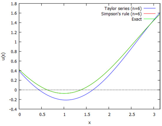
In Figure 1, Taylor series and Simpson’s rule solutions for $n=6$ are plotted and compared against the exact solution. The Simpson’s rule solution almost coincides with the exact solution. From Figure 1 and the results in Table 1 and Table 2, it is implied that Simpson’s rule approximate solutions converge very rapidly and at a constant rate to the true solution, while Taylor series approximation yields more accurate results when an adequate number of terms ($n=16$) are included in the truncated series.

Figure 1. Solution of integral Equation (42).

Example 2.

Consider the integral equation [5]

$$u\left(x\right)-\frac{1}{{\lambda }_A}{\int }_0^1{e}^{xt}u\left(t\right)dt=f\left(x\right),{\lambda }_A\ne 0,0\le x\le 1,$$

(48)

with

$$f\left(x\right)=e^x-\frac{e^{x+1}-1}{{\lambda }_A(x+1)},$$

so that (48) has the unique solution $u\left(x\right)=e^x$. The kernel $K(x,t)=e^{xt}$ is many times continuously differentiable on $[0,1]\times [0,1]$, but it is not separable. The input function $f\left(x\right)$ is continuous on $[0,1]$. We apply several approximating schemes.

DKM: Taylor series: 

We formulate the given integral equation as in (19). Specifically, we replace the kernel $K(x,t)$ and the input function $f\left(x\right)$ by finite segments of Taylor series of degree $n(r=n)$ about 0 in t and x, respectively, as follows

$$K_n(x,t)=\sum _{j=1}^{n+1}\frac{x^{j-1}}{(j-1)!}{t}^{j-1},f_n\left(x\right)=\sum _{j=1}^{n+1}{\left.\frac{d^{j-1}f\left(x\right)}{d{x}^{j-1}}\right|}_{x=0}{x}^{j-1},$$

and solve via (5) and (6). For ${\lambda }_A=2$, and $n=2$, we get

$$\begin{array}{ccc}\hfill {\tilde{u}}_2\left(x\right)& =& -\frac{2145e-7257}{1559}-\frac{(5184e-24420)x}{10913}-\frac{(4530e-17550)x^2}{10913}.\hfill \end{array}$$

Analogous solutions are obtained for other larger values of n; e.g., for $n=4$ and $n=8$, we have

$$\begin{array}{ccc}\hfill {\tilde{u}}_4\left(x\right)& =& 0.997193+0.998193x+0.499304x^2+0.166475x^3+0.041625x^4,\hfill \\ \hfill {\tilde{u}}_8\left(x\right)& =& 0.999999+0.999999x+0.499999x^2+0.166666x^3+0.041666x^4\hfill \\ & & +0.008333x^5+0.001388x^6+0.000198x^7+0.000024x^8.\hfill \end{array}$$

Comparison of these approximate solutions with the exact solution

$$u\left(x\right)=e^x=1+x+\frac{x^2}{2}+\frac{x^3}{6}+\frac{x^4}{24}+\frac{x^5}{120}+\frac{x^6}{720}+\frac{x^7}{5040}+\frac{x^8}{40320}+\dots$$

shows the excellent agreement accomplished even with small values of n. Further, the maximum errors between the approximate solutions for various values of n and the exact solution are given in Table 3. The maximum error is located at the point $x=1$ in all cases. The results are distinguished for their high accuracy.

Table 3. IE (48), ${\lambda }_A=2$. DKM: Taylor series.

n	${\mathit{ϵ}}_{\mathit{n}}={\parallel \mathit{u}-{\tilde{\mathit{u}}}_{\mathit{n}}\parallel }_{\mathit{\infty }}$	$\mathit{\eta }=\frac{{\mathit{ϵ}}_{\mathit{n}}}{\left|\mathit{u}\right|}$	$100\%\times \mathit{\eta }$	Ratio
2	3.77 × 10${}^{-1}$	1.39 × 10${}^{-1}$	13.88%
4	1.55 × 10${}^{-2}$	5.70 × 10${}^{-3}$	0.57%	24.3
8	4.14 × 10${}^{-6}$	1.52 × 10${}^{-6}$	1.52 × 10${}^{-4}$%	3.7 × 10${}^3$
16	3.62 × 10${}^{-15}$	1.33 × 10${}^{-15}$	1.33 × 10${}^{-13}$%	1.1 × 10${}^9$

DKM: Polynomials: 

We follow the procedure in Section 4.2 and approximate $K(x,t)$ and $f\left(x\right)$ with interpolating polynomials of degree n ($r=n$). Expressing the integral equation in (48) in the form (28) and solving by means of Theorem 1 for ${\lambda }_A=2$, we find

$$\begin{array}{ccc}\hfill {\tilde{u}}_2\left(x\right)& =& 1.003217+0.877792x+0.847809x^2,\hfill \\ \hfill {\tilde{u}}_4\left(x\right)& =& 1.000005+0.998808x+0.509797x^2+0.140256x^3+0.069434x^4,\hfill \\ \hfill {\tilde{u}}_8\left(x\right)& =& 1.000000+0.999999x+0.500000x^2+0.166664x^3+0.041675x^4\hfill \\ & & +0.008310x^5+0.001425x^6+0.000164x^7+0.000041x^8.\hfill \end{array}$$

Table 4 shows the maximum errors between these approximate solutions and the exact solution and the points where they occur. As expected, the results are very accurate. Compared with those obtained by the Taylor series above, they are superior. 

Table 4. IE (48), ${\lambda }_A=2$. DKM: Polynomials.

n	${\mathit{ϵ}}_{\mathit{n}}={\parallel \mathit{u}-{\tilde{\mathit{u}}}_{\mathit{n}}\parallel }_{\mathit{\infty }}$	$\mathit{\eta }=\frac{{\mathit{ϵ}}_{\mathit{n}}}{\left|\mathit{u}\right|}$	$100\%\times \mathit{\eta }$	${\mathit{x}}_{\mathbf{m}\mathbf{a}\mathbf{x}{\mathit{ϵ}}_{\mathit{n}}}$
2	2.26 × 10${}^{-2}$	9.99 × 10${}^{-3}$	1.00%	0.8150
4	6.98 × 10${}^{-5}$	2.80 × 10${}^{-5}$	2.80 × 10${}^{-3}$%	0.9150
8	2.17 × 10${}^{-10}$	8.28 × 10${}^{-11}$	8.28 × 10${}^{-9}$%	0.9625

QM: Trapezoidal rule and Taylor series: 

Let us use the composite trapezoidal rule

$${\int }_a^{b}y\left(x\right)dx\approx \frac{h}{2}\left\{y\left(x_1\right)+2\sum _{j=2}^{n}y\left(x_j\right)+y\left(x_{n+1}\right)\right\},$$

(49)

to approximate the integral in (48). Following the procedure in Section 5, we may initially express (48) in the form (34). However, to construct an explicit solution of a type such as a polynomial throughout the interval $[a,b]$, we substitute the components of the vector G and the function $f\left(x\right)$ with finite segments of the Taylor series of degree $r=n$ in x about 0, as in (36). After solving by means of (5) and (6) for ${\lambda }_A=2$, and $n=2$, we obtain the solution

$${\tilde{u}}_2\left(x\right)=-\frac{3436e-11712}{2391}-\frac{(1268e-5892)x}{2391}-\frac{(1096e-4248)x^2}{2391}.$$

Similarly, for $n=4$ and $n=8$, we acquire the higher order solutions

$$\begin{array}{ccc}\hfill {\tilde{u}}_4\left(x\right)& =& 1.026427+1.024317x+0.515273x^2+0.172608x^3+0.043388x^4,\hfill \\ \hfill {\tilde{u}}_8\left(x\right)& =& 1.007331+1.006523x+0.503972x^2+0.168193x^3+0.042106x^4\hfill \\ & & +0.008433x^5+0.001407x^6+0.000201x^7+0.000025x^8.\hfill \end{array}$$

The maximum errors between the approximate solutions corresponding to various values of n and the exact solution are listed in Table 5. Moreover, in Table 6, we give the results obtained when ${\lambda }_A=50$. It is evident that the accuracy is $O\left(h^2\right)$ in the entire interval $[0,1]$. As the value of the parameter ${\lambda }_A$ increases, the accuracy improves and the convergence to the exact solution is faster.

Table 5. IE (48), ${\lambda }_A=2$. QM: Trapezoidal rule and Taylor series.

n	${\mathit{ϵ}}_{\mathit{n}}={\parallel \mathit{u}-{\tilde{\mathit{u}}}_{\mathit{n}}\parallel }_{\mathit{\infty }}$	$\mathit{\eta }=\frac{{\mathit{ϵ}}_{\mathit{n}}}{\left|\mathit{u}\right|}$	$100\%\times \mathit{\eta }$	Ratio
2	1.73 × 10${}^{-1}$	6.36 × 10${}^{-2}$	6.36%
4	6.37 × 10${}^{-2}$	2.34 × 10${}^{-2}$	2.34%	2.7
8	1.99 × 10${}^{-2}$	7.33 × 10${}^{-3}$	0.73%	3.2
16	4.95 × 10${}^{-3}$	1.82 × 10${}^{-3}$	0.18%	4.0

Table 6. IE (48), ${\lambda }_A=50$. QM: Trapezoidal rule and Taylor series.

n	${\mathit{ϵ}}_{\mathit{n}}={\parallel \mathit{u}-{\tilde{\mathit{u}}}_{\mathit{n}}\parallel }_{\mathit{\infty }}$	$\mathit{\eta }=\frac{{\mathit{ϵ}}_{\mathit{n}}}{\left|\mathit{u}\right|}$	$100\%\times \mathit{\eta }$	Ratio
2	2.172 × 10${}^{-1}$	7.989 × 10${}^{-2}$	7.989%
4	8.710 × 10${}^{-3}$	3.204 × 10${}^{-3}$	0.320%	24.9
8	3.356 × 10${}^{-4}$	1.235 × 10${}^{-4}$	0.012%	26.0
16	8.473 × 10${}^{-5}$	3.117 × 10${}^{-5}$	0.003%	4.0

QM: Trapezoidal rule and Polynomials: 

Let us now consider the approximating scheme in (37) where we employ the composite trapezoidal rule to discritize the integral and interpolating polynomials of degree $r=n$ to approximate the components of G and the function $f\left(x\right)$. For ${\lambda }_A=2$, and $n=2$, $n=4$ and $n=8$, we obtain the corresponding solutions

$$\begin{array}{ccc}\hfill {\tilde{u}}_2\left(x\right)& =& 1.131517+0.972464x+0.969511x^2,\hfill \\ \hfill {\tilde{u}}_4\left(x\right)& =& 1.029984+1.025406x+0.526503x^2+0.145148x^3+0.072597x^4,\hfill \\ \hfill {\tilde{u}}_8\left(x\right)& =& 1.007331+1.006524x+0.503972x^2+0.168191x^3+0.042115x^4\hfill \\ & & +0.008410x^5+0.001444x^6+0.000167x^7+0.000041x^8.\hfill \end{array}$$

In Table 7, we list the maximum errors between these approximate solutions and the exact solution. Additionally, in Table 8, we present the results for the value of the parameter ${\lambda }_A=50$. The results are very close to those obtained above with the composite Trapezoidal rule and Taylor series.

Table 7. IE (48), ${\lambda }_A=2$. QM: Trapezoidal rule and Polynomials.

n	${\mathit{ϵ}}_{\mathit{n}}={\parallel \mathit{u}-{\tilde{\mathit{u}}}_{\mathit{n}}\parallel }_{\mathit{\infty }}$	$\mathit{\eta }=\frac{{\mathit{ϵ}}_{\mathit{n}}}{\left|\mathit{u}\right|}$	$100\%\times \mathit{\eta }$	Ratio
2	3.55 × 10${}^{-1}$	1.31 × 10${}^{-1}$	13.07%
4	8.14 × 10${}^{-2}$	2.99 × 10${}^{-2}$	2.99%	4.4
8	1.99 × 10${}^{-2}$	7.33 × 10${}^{-3}$	0.73%	4.1
16	4.95 × 10${}^{-3}$	1.82 × 10${}^{-3}$	0.18%	4.1

Table 8. IE (48), ${\lambda }_A=50$. QM: Trapezoidal rule and Polynomials.

n	${\mathit{ϵ}}_{\mathit{n}}={\parallel \mathit{u}-{\tilde{\mathit{u}}}_{\mathit{n}}\parallel }_{\mathit{\infty }}$	$\mathit{\eta }=\frac{{\mathit{ϵ}}_{\mathit{n}}}{\left|\mathit{u}\right|}$	$100\%\times \mathit{\eta }$	Ratio
2	5.351 × 10${}^{-3}$	1.968 × 10${}^{-2}$	0.197%
4	1.351 × 10${}^{-3}$	4.971 × 10${}^{-4}$	0.050%	4.0
8	3.387 × 10${}^{-4}$	1.246 × 10${}^{-4}$	0.012%	4.0
16	8.473 × 10${}^{-5}$	3.117 × 10${}^{-5}$	0.003%	4.0

PM: Collocation with Polynomials: 

Finally, we solve the integral equation in (48) by employing a projection method such as the simple collocation method given in Section 6, where the ordinary Lagrange basis functions are used. For ${\lambda }_A=1$, by means of (41) and polynomials of degree $n=3$, $n=4$ and $n=5$ interpolating $u\left(x\right)$ on the equally spaced nodes $x_j=(j-1)/n,j=1,2,\dots ,n+1$, we obtain the following solutions

$$\begin{array}{ccc}\hfill {\tilde{u}}_3\left(x\right)& =& 0.999256+1.013577x+0.425543x^2+0.278580x^3,\hfill \\ \hfill {\tilde{u}}_4\left(x\right)& =& 0.999985+0.998801x+0.509787x^2+0.140276x^3+0.069415x^4,\hfill \\ \hfill {\tilde{u}}_5\left(x\right)& =& 0.999998+1.000081x+0.499067x^2+0.170411x^3+0.0348642x^4\hfill \\ & & +0.013855x^5,\hfill \end{array}$$

respectively. In Table 9, we give the maximum errors between these approximate solutions and the exact solution. By way of illustration, we also compare these results with the maximum errors obtained in [24,25], where an advanced quasi-projection method based on B-spline tight framelets is utilized.

Table 9. IE (48), ${\lambda }_A=1$: PM: Collocation with Polynomials.

		[24] ${\mathit{ϵ}}_{\mathit{n}}={\parallel \mathit{u}-{\tilde{\mathit{u}}}_{\mathit{n}}\parallel }_2$				${\mathit{ϵ}}_{\mathit{n}}={\parallel \mathit{u}-{\tilde{\mathit{u}}}_{\mathit{n}}\parallel }_{\mathit{\infty }}$
$\mathit{n}$		${\mathit{N}}^{*}$	${\mathit{B}}_{\mathbf{2}}$-OEP	${\mathit{B}}_{\mathbf{4}}$-OEP		${\mathit{N}}^{*}$
2		40	1.03 × 10${}^{-3}$	4.45 × 10${}^{-7}$		3	1.96 × 10${}^{-2}$
3		112	1.08 × 10${}^{-4}$	1.78 × 10${}^{-7}$		4	1.47 × 10${}^{-3}$
4		288	1.25 × 10${}^{-4}$	4.35 × 10${}^{-8}$		5	6.02 × 10${}^{-5}$
5		704	9.78 × 10${}^{-5}$	1.58 × 10${}^{-9}$		6	2.87 × 10${}^{-6}$

*N = order of system of linear algebraic equations to solve.

Example 3.

Consider the integral equation

$$u\left(x\right)-\frac{1}{{\lambda }_A}{\int }_0^1\frac{cu\left(t\right)}{c^2+{(x-t)}^2}dt=f\left(x\right),0\le x\le 1,$$

(50)

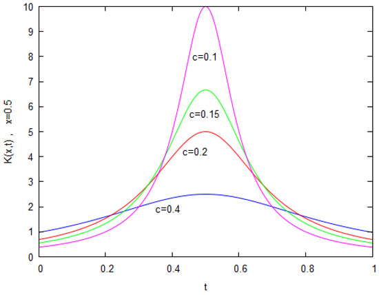
where the parameters ${\lambda }_A\ne 0$ and $c>0$. This equation appears in electrostatics and it is known as Love’s equation [26]. The kernel function

$$K(x,t)=\frac{c}{c^2+{(x-t)}^2},$$

(51)

is continuous on $[0,1]\times [0,1]$ with a peak at $x=t$ when c is small. Figure 2 shows the shape of $K(x,t)$ for various values of c and $x=0.5$. It is understood that as c diminishes to zero, the more difficult it is to construct the solution to the problem. Let ${\lambda }_A=-0.5$, $c=0.1$ and

$$\begin{array}{ccc}\hfill f\left(x\right)& =& \frac{1}{50}(10x-4)ln\left(\frac{100x^2-200x+101}{100x^2+1}\right)+\hfill \\ & & \frac{1}{50}(100x^2-80x+5)(arctan\left(10x\right)-arctan(10x-10))+\hfill \\ & & \frac{1}{50}(50x^2-40x+13),\hfill \end{array}$$

so that (50) has the exact solution $u\left(x\right)=0.06-0.8x+x^2$ [26].

Figure 2. Function $K(x,t)$ in (51), $x=0.5$.

We noticed that Taylor series and interpolation polynomials are not generally efficient in solving problems with kernel functions of the type (51) when c is small ($c<0.5$). Therefore, we apply here the quadrature method in Section 5 by using the Trapezoidal and Simpson’s rules.

QM: Trapezoidal rule: 

Let us consider $n+1$ equally spaced quadrature points $0=x_1<x_2<\dots <x_{n+1}=1$, $x_j=(j-1)h,j=1,2,\dots ,n+1,$ where $h=1/n$, in the interval $[0,1]$. We use the quadrature formula in (49) to approximate the integral in (50) and then, through the steps in Section 5, write Equation (50) in the form (34), i.e.,

$$T_q{\tilde{u}}_n={\tilde{u}}_n-G\mathrm{\Psi }\left({\tilde{u}}_n\right)=f,$$

(52)

where the vectors

$$G=-\frac{1}{n}\left(\begin{array}{cccc}\frac{1}{10\left(\frac{1}{100}+x^2\right)}& \frac{1}{5\left(\frac{1}{100}+{(x-x_2)}^2\right)}& \dots & \frac{1}{10\left(\frac{1}{100}+{(x-1)}^2\right)}\end{array}\right),\mathrm{\Psi }\left({\tilde{u}}_n\right)=\left(\begin{array}{c}{\tilde{u}}_n\left(0\right)\\ {\tilde{u}}_n\left(x_2\right)\\ ⋮\\ {\tilde{u}}_n\left(1\right)\end{array}\right).$$

Solving (52) via (5) and (6), we obtain an approximate analytic solution to (50) in the interval $[0,1]$. For example, for $n=2$, we have

$${\tilde{u}}_2\left(x\right)=f\left(x\right)-\frac{4.052649\times {10}^{-4}}{0.01+x^2}+\frac{0.004199}{0.01+{(x-0.5)}^2}-\frac{0.005479}{0.01+{(x-1.0)}^2}.$$

In Table 10, we record the maximum errors for various values of n. The maximum error occurs at the point $x=1$ except in the instance $n=8$, which is a poor approximation anyway, where it is located at $x=0.935$.

Table 10. IE (50), ${\lambda }_A=-0.5$, $c=0.1$. QM: Trapezoidal rule.

n	${\mathit{ϵ}}_{\mathit{n}}={\parallel \mathit{u}-{\tilde{\mathit{u}}}_{\mathit{n}}\parallel }_{\mathit{\infty }}$	$\mathit{\eta }=\frac{{\mathit{ϵ}}_{\mathit{n}}}{\left|\mathit{u}\right|}$	$100\%\times \mathit{\eta }$	Ratio
8	5.20 × 10${}^{-2}$	2.79 × 10${}^{-1}$	27.95%
16	7.32 × 10${}^{-3}$	2.82 × 10${}^{-2}$	2.82%
32	2.02 × 10${}^{-3}$	7.78 × 10${}^{-3}$	0.78%	3.6
64	5.16 × 10${}^{-4}$	1.98 × 10${}^{-3}$	0.20%	3.9
128	1.30 × 10${}^{-4}$	4.98 × 10${}^{-4}$	0.05%	4.0

QM: Simpson’s rule: 

We utilize now the quadrature formula in (45), with n being an even number, and repeat the steps above. As an illustration, for $n=16$, we obtain the solution

$$\begin{array}{ccc}\hfill {\tilde{u}}_{16}\left(x\right)& =& f\left(x\right)-\frac{2.554573\times {10}^{-4}}{x^2+0.01}-\frac{2.269247\times {10}^{-4}}{{(x-0.0625)}^2+0.01}+\frac{2.119289\times {10}^{-4}}{{(x-0.125)}^2+0.01}\hfill \\ & & +\frac{8.937448\times {10}^{-4}}{{(x-0.1875)}^2+0.01}+\frac{6.691821\times {10}^{-4}}{{(x-0.25)}^2+0.01}+\frac{0.001507}{{(x-0.3125)}^2+0.01}+\frac{8.573774\times {10}^{-4}}{{(x-0.375)}^2+0.01}\hfill \\ & & +\frac{0.001609}{{(x-0.4375)}^2+0.01}+\frac{7.766917\times {10}^{-4}}{{(x-0.5)}^2+0.01}+\frac{0.001200}{{(x-0.5625)}^2+0.01}+\frac{4.271220\times {10}^{-4}}{{(x-0.625)}^2+0.01}\hfill \\ & & +\frac{2.803521\times {10}^{-4}}{{(x-0.6875)}^2+0.01}-\frac{1.912995\times {10}^{-4}}{{(x-0.75)}^2+0.01}-\frac{0.001151}{{(x-0.8125)}^2+0.01}-\frac{0.001080}{{(x-0.875)}^2+0.01}\hfill \\ & & -\frac{0.003089}{{(x-0.9375)}^2+0.01}-\frac{0.001106}{{(x-1.0)}^2+0.01}.\hfill \end{array}$$

Table 11 shows the errors of the approximate solutions for varying values of n. It is noted that the maximum error occurs at the point $x=1$, with the exception of the instances $n=8$ and $n=16$, where it is located at the points $x=0.95$ and $x=0.995$, respectively. In the same Table, some results obtained in [26] are also quoted for comparison. The supremacy of the Simpson’s rule is reaffirmed and the agreement with results of other formulations is acknowledged.

Table 11. IE (50), ${\lambda }_A=-0.5$, $c=0.1$. QM: Simpson’s rule.

n	[26] ${\mathit{ϵ}}_{\mathit{n}}={\parallel \mathit{u}-{\tilde{\mathit{u}}}_{\mathit{n}}\parallel }_{\mathit{\infty }}$	${\mathit{ϵ}}_{\mathit{n}}={\parallel \mathit{u}-{\tilde{\mathit{u}}}_{\mathit{n}}\parallel }_{\mathit{\infty }}$	$\mathit{\eta }=\frac{{\mathit{ϵ}}_{\mathit{n}}}{\left|\mathit{u}\right|}$	$100\%\times \mathit{\eta }$	Ratio
8		6.855 × 10${}^{-2}$	3.385 × 10${}^{-1}$	33.850%
16		5.630 × 10${}^{-3}$	2.216 × 10${}^{-2}$	2.216%
32		1.679 × 10${}^{-4}$	6.456 × 10${}^{-4}$	0.065%
64	6.6 × 10${}^{-6}$	6.636 × 10${}^{-6}$	2.552 × 10${}^{-5}$	0.003%	25.3

Example 4.

Consider the integral equation [8]

$$u\left(x\right)-{\int }_{-1}^1(x{t}^2-x^{2}t)dt=-x^4,x\in [-1,1].$$

(53)

The kernel $K(x,t)=x{t}^2-x^{2}t$ is continuous on $[-1,1]$ and separable. Thus, Equation (53) can be solved exactly by the DCM in Section 3 to obtain

$$u\left(x\right)=-\frac{30}{133}x+\frac{20}{133}{x}^2-x^4.$$

(54)

We also solve this equation here by the collocation method (PM) explained in Section 6. Specifically, we use Lagrange interpolating polynomials of the type (38) to approximate $u\left(x\right)$ and put the integral equation in (53) in the symbolic form (41). For $n=2$, $n=3$ and $n=4$, we obtain

$$\begin{array}{ccc}\hfill {\tilde{u}}_2\left(x\right)& =& -\frac{6}{19}x-\frac{15}{19}{x}^2,\hfill \\ \hfill {\tilde{u}}_3\left(x\right)& =& \frac{1}{9}-\frac{50}{171}x-\frac{470}{513}{x}^2,\hfill \\ \hfill {\tilde{u}}_4\left(x\right)& =& -\frac{30}{133}x+\frac{20}{133}{x}^2-x^4,\hfill \end{array}$$

respectively. Notice that for $n=4$, as expected, the exact solution was fully recovered. This further validates the procedure in Section 6.

Example 5.

Let the integral equation [9]

$$u\left(x\right)-\lambda {\int }_0^{2\pi }{e}^{i(x-t)}u\left(t\right)dt=e^x,x\in [0,2\pi ].$$

(55)

The kernel $K(x,t)=e^{i(x-t)}$ is continuous on $[0,2\pi ]$ and separable, and therefore the integral equation in (55) can be written as

$$u\left(x\right)-\lambda e^{ix}{\int }_0^{2\pi }{e}^{-it}u\left(t\right)dt=e^x.$$

(56)

Following the steps in DCM in Section 3, we set

$$G=\lambda e^{ix},\mathrm{\Psi }\left(u\right)={\int }_0^{2\pi }{e}^{-it}u\left(t\right)dt,$$

and write (56) in the form (14). By means of (5), $det\mathbf{V}=1-2\pi \lambda$, and hence the integral Equation (55) has a unique solution if $\lambda \ne \frac{1}{2\pi }$. In this case by substituting into (6), we obtain the unique solution

$$u\left(x\right)=e^x+\frac{\lambda (1+i)(e^{2\pi }-1)}{2(1-2\pi \lambda )}{e}^{ix},\lambda \ne \frac{1}{2\pi }.$$

8. Discussion

The main objective of the present article was to present a unified and versatile procedure suitable for symbolic computations for the construction of approximate analytic solutions to linear Fredholm integral equations of the second kind with general continuous kernels.

It was shown how some of the classical methods such as the Direct Computational Method (DCM), the Degenerate Kernel Methods (DKM), the Quadrature Methods (QM) and the Projection Methods (PM) can be incorporated in the proposed procedure. Additionally, it was demonstrated how complicated calculations such as double power series approximation, interpolation in two dimensions and combinations of different types of approximation can be handled in an effective way.

The technique was tested by solving several examples from the literature. Several approximating schemes for the kernel and the integral operator were used and their accuracy and convergence were evaluated.

In all cases, explicit solutions of high accuracy for the entire interval $[a,b]$ were obtained, which converge to the true solution as n increases. The power series approximation and polynomial interpolation of the kernel yield excellent results when the kernel is smooth with no “peaks”. For continuous kernels with “peaks” or kernels of the convolution type, numerical integration of the integral operator is appropriate.

In this paper, the emphasis was on presenting a novel framework for solving integral equations and on establishing its versatility and reliability in practice. A proper convergence and error analysis is postponed to a sequel paper. In the proposed framework, other numerical methods such as piecewise projection methods, Galerkin methods and wavelets methods can be included. The technique can be extended to two or more dimensions.

References

- Bystricky, L.; Pålsson, S.; Tornberg, A.-K. An accurate integral equation method for Stokes flow with piecewise smooth boundaries. BIT Numer. Math. 2021, 61, 309–335. [Google Scholar] [CrossRef]
- Selvadurai, A.P.S. The Analytical Method in Geomechanics. Appl. Mech. Rev. 2007, 404, 87–106. [Google Scholar] [CrossRef]
- Siedlecki, J.; Ciesielski, M.; Blaszczyk, T. Transformation of the second order boundary value problem into integral form - different approaches and a numerical solution. J. Appl. Math. Comput. Mech. 2015, 14, 103–108. [Google Scholar] [CrossRef]
- Atkinson, K.; Han, W. Boundary Integral Equations. In Theoretical Numerical Analysis: A Functional Analysis Framework; Springer: New York, NY, USA, 2005; pp. 523–553. [Google Scholar] [CrossRef]
- Atkinson, K.E. The Numerical Solution of Integral Equations of the Second Kind; Cambridge University Press: Cambridge, UK, 1997. [Google Scholar] [CrossRef]
- Kress, R. Linear Integral Equations: Third Edition; Springer: New York, NY, USA, 2014. [Google Scholar] [CrossRef]
- Polyanin, P.; Manzhirov, A.V. Handbook of Integral Equations: Second Edition, 2nd ed.; Chapman and Hall/CRC: New York, NY, USA, 2008. [Google Scholar] [CrossRef]
- Wazwaz, A.M. Linear and Nonlinear Integral Equations, 3rd ed.; Springer: Berlin, Germany, 2011. [Google Scholar] [CrossRef]
- Zemyan, S.M. The Classical Theory of Integral Equations; Birkhäuser: Basel, Switzerland, 2012. [Google Scholar] [CrossRef]
- Kumar, S.; Sloan, I.H. A New Collocation-Type Method for Hammerstein Integral Equations. Math. Comput. 1987, 48, 585–593. [Google Scholar] [CrossRef]
- Sloan, I.H.; Burn, B.J.; Datyner, N. A new approach to the numerical solution of integral equations. J. Comput. Phys. 1975, 18, 92–105. [Google Scholar] [CrossRef]
- Sloan, I.H.; Noussair, E.; Burn, B.J. Projection methods for equations of the second kind. J. Math. Anal. Appl. 1979, 69, 84–103. [Google Scholar] [CrossRef][Green Version]
- Allouch, C.; Remogna, S.; Sbibih, D.; Tahrichi, M. Superconvergent methods based on quasi-interpolating operators for fredholm integral equations of the second kind. Appl. Math. Comput. 2021, 404, 126227. [Google Scholar] [CrossRef]
- Baiburin, M.M.; Providas, E. Exact solution to systems of linear first-order integro-differential equations with multipoint and integral conditions. In Mathematical Analysis and Applications; Rassias, T., Pardalos, P., Eds.; Springer Optimization and Its Applications; Springer: Cham, Switzerland, 2019; Volume 154, pp. 1–16. [Google Scholar] [CrossRef]
- Dellwo, D.R. Accelerated degenerate-kernel methods for linear integral equations. J. Comput. Appl. Math. 1995, 58, 135–149. [Google Scholar] [CrossRef]
- Fairbairn, A.I.; Kelmanson, M.A. Spectrally accurate Nyström-solver error bounds for 1-D Fredholm integral equations of the second kind. Appl. Math. Comput. 2017, 315, 211–223. [Google Scholar] [CrossRef]
- Gao, R.X.; Tan, S.R.; Tsang, L.; Tong, M.S. A Nyström Method with Lagrange’s Interpolation for Solving Electromagnetic Scattering by Dielectric Objects. In Proceedings of the 2019 PhotonIcs Electromagnetics Research Symposium—Spring (PIERS-Spring), Rome, Italy, 17–20 June 2019; pp. 1957–1960. [Google Scholar] [CrossRef]
- Li, X.Y.; Wu, B.Y. Superconvergent kernel functions approaches for the second kind Fredholm integral equations. Appl. Numer. Math. 2021, 167, 202–210. [Google Scholar] [CrossRef]
- Molabahrami, A. The relationship of degenerate kernel and projection methods on Fredholm integral equations of the second kind. Commun. Numer. Anal. 2017, 2017, 34–39. [Google Scholar] [CrossRef][Green Version]
- Parasidis, I.N.; Providas, E. Resolvent operators for some classes of integro-differential equations. In Mathematical Analysis, Approximation Theory and Their Applications; Rassias, T., Gupta, V., Eds.; Springer Optimization and Its Applications; Springer: Cham, Switzerland, 2016; Volume 111, pp. 535–558. [Google Scholar] [CrossRef]
- Providas, E. Approximate solution of Fredholm integral and integro-differential equations with non-separable kernels. In Approximation and Computation in Science and Engineering; Daras, N.J., Rassias, T.M., Eds.; Springer Optimization and Its Applications 180; Springer: Berlin, Germany, 2021; pp. 697–712. [Google Scholar] [CrossRef]
- Conte, S.D.; De Boor, C. Elementary Numerical Analysis: An Algorithmic Approach; SIAM: New York, NY, USA, 2017. [Google Scholar] [CrossRef]
- Ramm, A.G. Integral Equations and Applications; Cambridge University Press: Cambridge, UK, 2015. [Google Scholar]
- Mohammad, M. A Numerical Solution of Fredholm Integral Equations of the Second Kind Based on Tight Framelets Generated by the Oblique Extension Principle. Symmetry 2019, 11, 854. [Google Scholar] [CrossRef]
- Mohammad, M.; Trounev, A.; Alshbool, M. A Novel Numerical Method for Solving Fractional Diffusion-Wave and Nonlinear Fredholm and Volterra Integral Equations with Zero Absolute Error. Axioms 2021, 10, 165. [Google Scholar] [CrossRef]
- Atkinson, K.E.; Shampine, L. Algorithm 876: Solving Fredholm Integral Equations of the Second Kind in Matlab. ACM Trans. Math. Softw. 2008, 34, 1–20. [Google Scholar] [CrossRef]
Publisher’s Note: MDPI stays neutral with regard to jurisdictional claims in published maps and institutional affiliations. |
© 2021 by the author. Licensee MDPI, Basel, Switzerland. This article is an open access article distributed under the terms and conditions of the Creative Commons Attribution (CC BY) license (https://creativecommons.org/licenses/by/4.0/).