Article

Short-Term Firm-Level Energy-Consumption Forecasting for Energy-Intensive Manufacturing: A Comparison of Machine Learning and Deep Learning Models

by
Andrea Maria N. C. Ribeiro
1,
Pedro Rafael X. do Carmo
1,
Iago Richard Rodrigues
1,
Djamel Sadok
1,
Theo Lynn
2 and
Patricia Takako Endo
3,*
1
Centro de Informática, Universidade Federal de Pernambuco, Pernambuco 50670-901, Brazil
2
Irish Institute of Digital Business, Dublin City University, 9 Dublin, Ireland
3
Programa de Pós-Graduação em Engenharia da Computação, Universidade de Pernambuco, Pernambuco 50100-010, Brazil
*
Author to whom correspondence should be addressed.
Algorithms 2020, 13(11), 274; https://doi.org/10.3390/a13110274
Submission received: 20 September 2020 / Revised: 23 October 2020 / Accepted: 28 October 2020 / Published: 30 October 2020

Abstract

:
To minimise environmental impact, to avoid regulatory penalties, and to improve competitiveness, energy-intensive manufacturing firms require accurate forecasts of their energy consumption so that precautionary and mitigation measures can be taken. Deep learning is widely touted as a superior analytical technique to traditional artificial neural networks, machine learning, and other classical time-series models due to its high dimensionality and problem-solving capabilities. Despite this, research on its application in demand-side energy forecasting is limited. We compare two benchmarks (Autoregressive Integrated Moving Average (ARIMA) and an existing manual technique used at the case site) against three deep-learning models (simple Recurrent Neural Networks (RNN), Long Short-Term Memory (LSTM), and Gated Recurrent Unit (GRU)) and two machine-learning models (Support Vector Regression (SVR) and Random Forest) for short-term load forecasting (STLF) using data from a Brazilian thermoplastic resin manufacturing plant. We use the grid search method to identify the best configurations for each model and then use Diebold–Mariano testing to confirm the results. The results suggests that the legacy approach used at the case site is the worst performing and that the GRU model outperformed all other models tested.

1. Introduction

The industrial sector is the largest consumer of delivered energy worldwide, and energy-intensive manufacturing is the largest component in that sector [1]. Energy-intensive manufacturing includes the manufacture of food, beverage, and tobacco products; pulp and paper; basic chemicals; refining; iron and steel; nonferrous metals, and nonmetallic metals [2]. Energy-intensity is driven by the mix of activity in these sectors including basic chemical feed-stocks; process (including heating and cooling) and assembly; steam and cogeneration; and building-related energy consumption, e.g., lighting, heating, and air conditioning [2]. World industrial energy consumption is forecasted to grow from c. 242 quadrillion British thermal units (Btu) in 2018 to about 315 quadrillion Btu in 2050; the proportion of energy-intensive manufacturing is forecasted to remain at approx. 50% during that period [1].
It is widely held that energy consumption tends to be positively associated with a higher rate of economic growth [3]; however, against this backdrop is the environmental impact of this consumption. As part of the United Nations Sustainable Development Goals (SDG), SDG 9 has industrial targets to reduce carbon dioxide (CO2) emission per unit of value added through increased resource-use efficiency and greater adoption of clean and environmentally sound technologies and industrial processes [4]. To meet these targets, governments worldwide are imposing regulations and taxes to reduce the environmental impact of industrial energy consumption. Firm-level forecasts of energy consumption are essential for precautionary and mitigation measures decision-making by management to minimise environmental impact, to manage cash flow, and to reduce or eliminate risk [5]. Accurate firm-level monitoring can also improve the data quality available to policymakers for local, regional, and national policies and actions.
Extant literature has typically (i) focused on supply-side perspectives, (ii) aggregated energy costs, and (iii) failed to recognise the idiosyncrasies of the energy-intensive manufacturing sector and the associated centrality of energy management in production planning. There is a paucity of studies in demand-side process-related short-term load forecasting (STLF) using deep learning and machine learning for energy-intensive manufacturing. The limited studies that have been published do not compare deep-learning performance against widely used machine-learning models, classical time series models, or approaches used in practice. In addition to proposing prediction models, we also address this gap.
In this paper, we focus on performance analyses of deep-learning and machine-learning models for firm-level STLF considering the energy-intensive manufacturing process of a thermoplastic resin manufacturer. We use energy consumption and production flow data from a real Brazilian industrial site. In addition to the energy consumption time series, we use data from two different stages of the thermoplastic resin production process: polymerisation and solid-state polymerisation. We propose three deep-learning models—simple Recurrent Neural Networks (RNN), Long Short-Term Memory (LSTM) networks, and Gated Recurrent Unit (GRU)—and two machine-learning models—Support Vector Regression (SVR) and Random Forest—for predicting daily energy consumption. These techniques were selected as they are referenced in the literature on STLF for demand-side energy consumption [6,7]. We use the grid search method to identify the best model configurations. We compare the performance of the deep-learning and machine-learning models against (i) a classical time series model, Autoregressive Integrated Moving Average (ARIMA), and (ii) the current manual approach at the case site.
The remainder of this paper is organised as follows. Section 2 presets the description of the data, preprocessing, and evaluation metrics used in our work. Section 3 presents the models identified for evaluation. Our results and most relevant findings are discussed in Section 4. Section 5 presents a discussion about the related works. The paper concludes with a summary of the paper and future avenues for research in Section 6.

2. Material and Method

2.1. Dataset

The data used in this study was sourced from the Brazilian subsidiary of an international thermoplastic resin manufacturer, an energy-intensive manufacturing plant. The plant size is c. 55,000 m2 with a production capacity of approximately 500,000 tons per year. Currently, the case site calculates energy consumption forecasts manually and prepares a technical energy consumption index (TECI) as a proxy for energy efficiency. Five years of data from 1 January 2015 to 31 December 2019 for daily total energy consumption at the plant (ENERGY dataset) as well as process-related data for two different stages of the manufacturing process—polymerisation (POLY_PRODUCTION dataset) and solid-state polymerisation (SSPOLY_PRODUCTION dataset)—were provided. Each dataset comprised 1826 values. Figure 1 presents the time series of the three datasets used in this work.
To identify the impact of the variations in the production flow data on total plant energy consumption, we performed a Pearson correlation analysis. It showed a moderate positive correlation between the ENERGY dataset and the combined production flow dataset (POLY_PRODUCTION dataset and SSPOLY_PRODUCTION dataset). The correlation coefficient between the ENERGY dataset and the POLY_PRODUCTION dataset was 0.71, while the relationship between the ENERGY dataset and the SSPOLY_PRODUCTION dataset was 0.75. Once this analysis was completed, a decision was made to include all three time series (ENERGY, POLY_PRODUCTION, SSPOLY_PRODUCTION) as input in the deep-learning models.

2.2. Data Preprocessing

Missing values and measurement errors can lead to unpredictable results. To avoid removing these, anomalous data were filled with imputed data and then normalised. For the former, we replaced missing data with the average of the data from the previous seven days as per [8,9,10]. We then normalised the data so that all model inputs had equal weights and the Sigmoid activation function could be applied in the deep-learning models as per [11,12,13]. Normalization reduces the data range to zero and one [0, 1]. Sklearn’s MinMaxScaler function was used to normalise the data in this study, based on Equation (1).
X i = X i m i n ( x ) m a x ( x ) m i n ( x )
where X i is the rescaled value, X i is the original value, min(x) is the minimum value in feature, and max(x) is the maximum value in feature.

2.3. Evaluation Metric

Root mean squared error (RMSE), mean absolute percent error (MAPE), and mean absolute error (MAE) are the most commonly metrics used in the evaluation of the accuracy of energy-consumption models [14] and, in particular, studies related to STLF using deep learning [6,7,15].
RMSE is defined as the square root of the mean squared error (MSE) [16] (Equation (2) [17]), that is, the root of the mean square error of the difference between the prediction ( P i ) and the real value ( R i ), where n is sample size. As RMSE is more sensitive to more significant errors (outliers) because it squares the difference between the predicted value and the real value. RMSE presents error values in the same dimensions as the analysed variable [16]. It is widely applied in models that use time series [18].
R M S E = 1 n i = 1 n ( P i R i ) 2
MAPE is widely used for evaluating prediction models particularly where the quality of the forecast is required and is used in numerous energy-consumption forecasting studies [6,11,12,13,19]. MAPE is defined in Equation (3) [6,11,17] and expresses the accuracy of the error as a percentage. It can be applied in a wide range of contexts, as it is a relatively intuitive interpretation of relative errors; however, it can only be used if the values in the dataset do not equal zero [20].
M A P E % = 100 n i = 1 n P i R i R i
MAE is defined in Equation (4) [12,17]. Unlike the other metrics presented, MAE depends on the scale of the data. It is not sensitive to outliers, as it treats all errors in the same way. We use it to quantify a model’s ability to predict energy consumption.
M A E = 1 n i = 1 n P i R i
While one or more of RMSE, MAPE, and MAE have been featured in related studies [6,7], we have chosen to measure all of them for better comprehensiveness and analysis of different aspects of what is being studied [21].

3. Finding Models to Predict Energy Consumption

Due to the nonlinear characteristics of the datasets used in this research, to the need for both accuracy and fast run times, and to the promising results obtained in other works that used deep learning [12,19,22,23], three deep-learning techniques were selected for STLF in this study: simple RNN, LSTM, and GRU. In addition to these techniques, two different machine-learning techniques were selected for the purpose of comparison: SVR, and Random Forest. These were selected as they are featured in related works on STLF for demand-side energy consumption [6,7]. Our models use three time series as input—(i) energy consumption, (ii) polymerisation production flow (POLY), and (iii) solid-state polymerisation production flow (SSPOLY)—and have a single output: the predicted energy consumption. For each input, the model uses data from the preceding seven days.

3.1. Deep Learning Models

As mentioned previously, we propose three deep-learning techniques for STLF: simple RNN, LSTM, and GRU. RNNs are a type of Artificial Neural Network (ANN) designed to recognise patterns in sequential data streams. In RNNs, the decision, classification, or learning done at a given moment t−1 influence the decision, classification, or learning at a subsequent time t in the time series. RNNs contain two sources of input: the present and the recent past. These data are combined to determine how new data is predicted. RNNs have a memory that, for example, multi-layer perceptrons (MLP) and Convolutional Neural Network (CNN) do not. As such, RNNs use information in the sequence itself to perform tasks that other ANNs are unable to do. RNNs have limitations, the most significant of which are difficulties in training RNNs to capture long-term dependencies due to vanishing and exploding gradient problems [24,25]. LSTM and GRU are variations of RNN that overcome such problems.
LSTM [26] is a variation of RNN that overcomes gradient problems through the use of a chain structure containing four neural networks and different blocks of memory [27]. LSTM updates its unit states using three gates: a forget gate, an input gate, and an output gate. The forget gate deletes information that is no longer useful in the unit [27]. The current input x t and the output from the previous unit h t 1 are multiplied by the weight matrix. The result is passed through an activation function that provides a binary output that causes the data to be forgotten. The input gate performs addition of useful information to the unit’s status. First, the information is adjusted using a sigmoid function. Then, the tanh function is used to create a vector that produces 1 to + 1 . Finally, the output gate completes the extraction of useful information from the current state of the unit to be displayed as an output. In order to do so, a vector is generated by applying a tanh function to a cell. Due to its structure, LSTMs can predict time series with time intervals of unknown duration [28], a significant advantage over traditional RNNs. Notwithstanding this, long training times are a significant limitation [29].
GRUs reduce the complexity of LSTMs by only utilising an update gate and a reset gate to determine how values in the hidden states are computed [25]. In GRUs, only one hidden state is transferred between the time steps [25]. This state is capable of maintaining long- and short-term dependencies at the same time. GRU gates are trained to selectively filter out any irrelevant information while maintaining what is useful. These gates are vectors containing binary values, as in LSTM, and determine the importance of the information. Crucially, research suggests that GRUs have significantly faster training times with comparable performance to LSTM [25,29].

Deep Learning Model Settings

To determine the most suitable configuration for each deep-learning model, we use the grid search method to determine the respective hyperparameters [30,31,32,33,34]. It is used widely as it is quick to implement, is trivial to parallelise, and intuitively allows an entire search space to be explored [35].
To perform the grid search, the dataset was separated into a training set consisting of 80% of the original dataset (from 1 January 2015 to 30 December 2018) and a test set comprising 20% of the original dataset (from 31 December 2018 to 31 December 2019) using percentage split. The hyperparameters evaluated by the grid search for deep-learning techniques were (i) the number of layers, and (ii) the number of nodes in each layer (see Table 1).
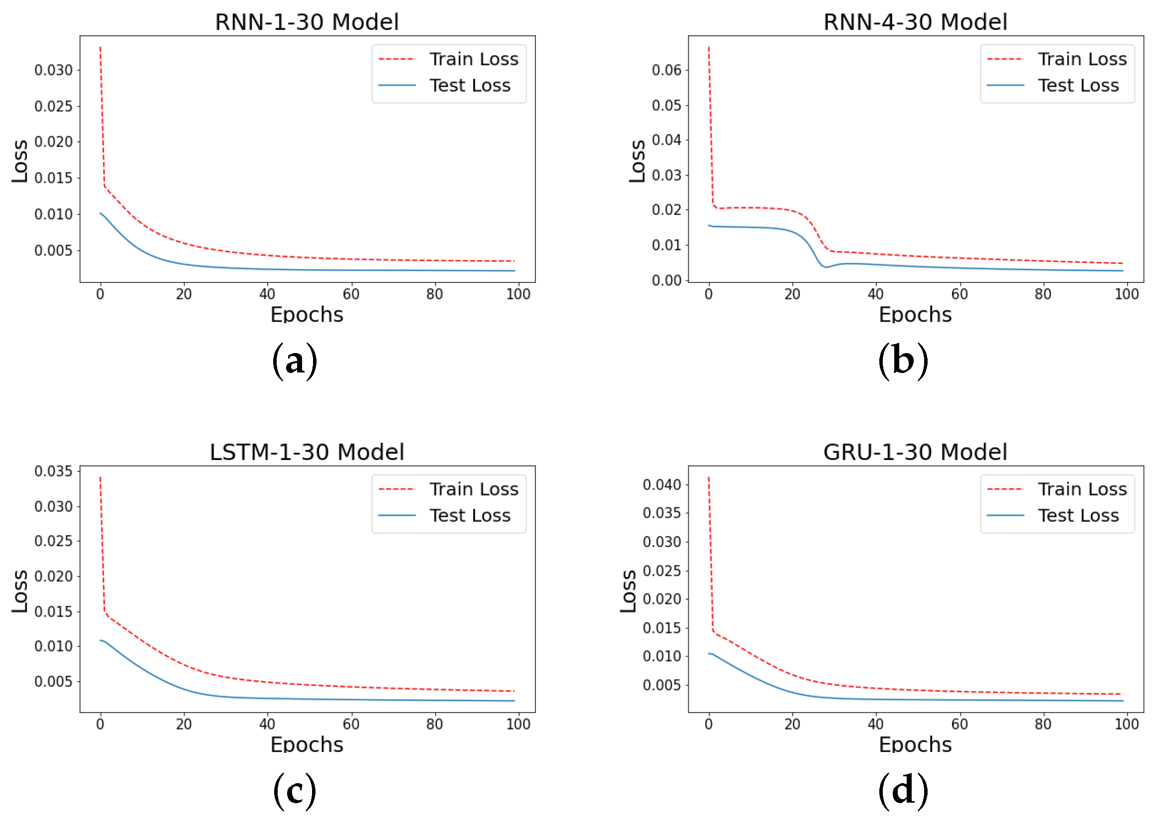
Figure 2 presents the loss convergence during both training and testing of the deep-learning models. It suggests that the models converge after about 40 epochs (loss stabilisation); there is no overfitting.
For deep-learning models, the following parameters were fixed: 100 epochs based on (Figure 2), a batch size of 16, Sigmoid [36] as the activation function, MSE as the loss function, and a method for stochastic optimisation (Adam) as the optimiser. These parameters were chosen empirically. Due to the stochastic nature of the optimisation process, the grid search was performed 30 times, and the averages of RMSE, MAPE, and MAE were calculated.
Figure 3, Figure 4 and Figure 5 present the grid search normalised results for RMSE, MAPE, and MAE, respectively. The configuration with one layer and 30 nodes generated the best models—RNN-1-30, LSTM-1-30, and GRU-1-30—for all deep-learning techniques, except in one instance where the average MAPE presented the best result for RNN with a configuration of four layers and 30 nodes, i.e., RNN-4-30. These four model configurations will be used in our benchmark evaluation.
As model complexity increases, deep-learning models learn more from the greater volume of available data in the training dataset.

3.2. Machine-Learning Models

In addition to deep-learning models, we also propose two machine-learning models: SVR and Random Forest.
Support Vector Machines (SVM) has been proposed as an alternative to traditional ANNs for classification and regression tasks. In particular, SVM provides better support for forecasting time series from nonlinear systems [37]. SVM is a machine-learning technique based on statistical learning theory [38]. Extant literature suggests that SVM performs well in forecasting time series [37,39,40]. Support Vector Regression (SVR) is a regression technique based on SVM [41]. The main differences relate to the formats and types of input and output. Kernel functions are used to map the data through nonlinear functions in an n-dimensional space. In this way, it is possible to transform nonlinear problems into linear problems. Research suggests that SVR presents accurate results for predicting energy consumption and, as such, is commonly used in the field [42]. Despite its advantages, the lack of predetermined heuristics for both the design and parameterisation of SVR models is a major drawback in using SVR [37]. As such, studies tend to be application-specific and to lack generalisability [37].
Random Forest is a machine-learning technique based on different decision trees. Random Forests’ implementation involves random selection of features based on the position of the root node. The model output consists of the average of the results for all trees. When compared to a single decision tree, Random Forest presents a better performance [43,44,45]. The greater the number of trees, normally the better the performance of the model but the slower the model and the more inefficient the real-time predictions. It is one of the most popular machine-learning techniques used for classification and regression problems [21,46,47]. Random Forest’s popularity is often attributed to its higher accuracy when compared with ANNs and SVR [48].

Machine-Learning Model Settings

Similar to the deep-learning models, we also perform grid search to find the best hyperparameters of the machine-learning models, using the same data set splitting procedure. The hyperparameters used vary according to the technique (see Table 2). For SVR, cost and the type of kernel were used, whereas the maximum depth of trees and the number of trees were used for Random Forest.
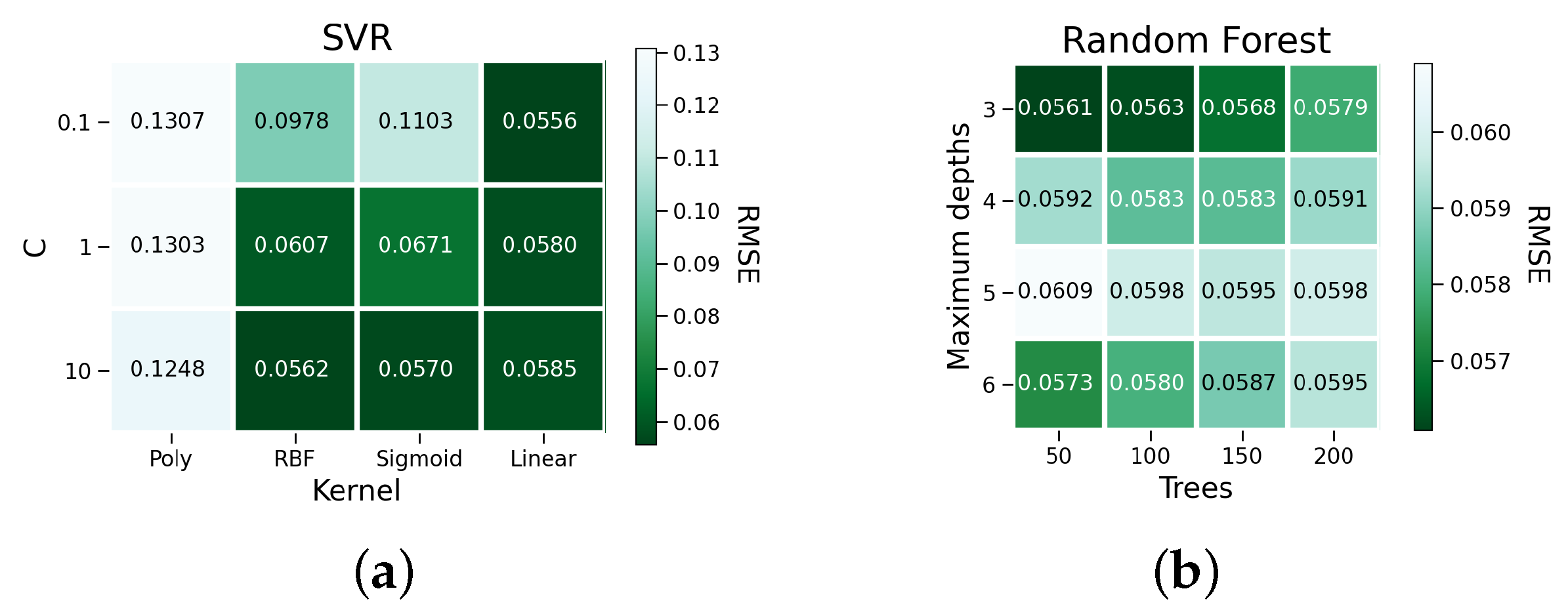
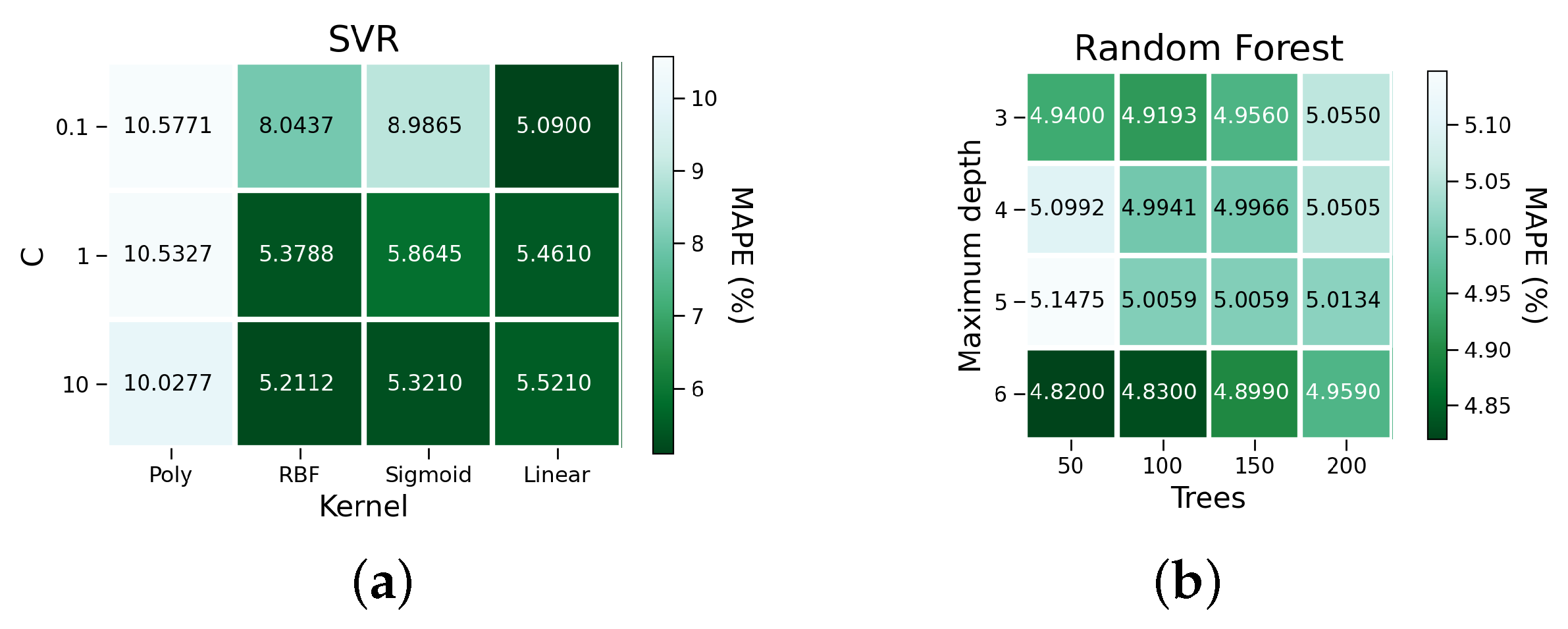
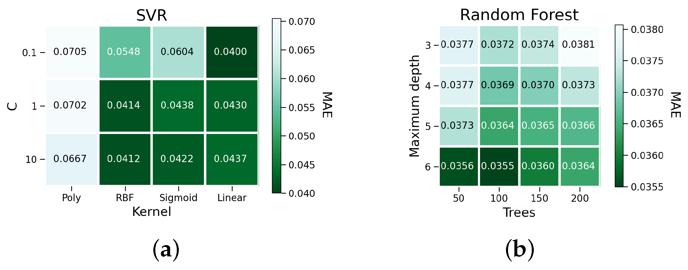
Figure 6, Figure 7 and Figure 8 present the grid search results for RMSE, MAPE, and MAE, respectively. For SVR, the best configuration across the three metrics used—RMSE, MAPE, and MAE—is represented by SVR-0.1-linear, for which the C value is 0.1 and used the linear kernel. For Random Forest, the models with configurations with (a) a maximum depth of three with 50 trees (Random Forest-3-50), (b) maximum depth of six with 50 trees (Random Forest-6-50), and (c) a maximum depth of six with 100 trees (Random Forest-6-100) generated the best results for RMSE, MAPE, and MAE, respectively. These four model configurations will be used in our benchmark evaluation.

3.3. Benchmarks

Two additional benchmarks were selected for comparison purposes. The first benchmark is the manual technique used by the case site providing the dataset for this study. The second benchmark is an ARIMA model. ARIMA was selected because of its widespread use in energy forecasting and, in particular, in related works [6].
The manual technique used by the case site is performed by a simple calculation as per Equation (5), where the energy consumption of a given day, C p r e d i c t e d , is the planned production flow ( F p l a n n e d ) and the TECI ( n p r e v i o u s ) based on measured data collected on the previous day.
C p r e d i c t e d = F p l a n n e d n p r e v i o u s
The choice of the ARIMA model for this study was based on the time-series nature of our dataset (data numbers and the output variable relates to your past data). Equation (6) [49] represents the mathematical expression for the autoregressive part.
x ( t ) = i = 1 p α i x ( t i )
where t is the index represented by an integer, x ( t ) is the estimated value, p is the number of autoregressive terms, and α is the polynomial related to the autoregressive operator of order p.
Equation (7) [49] reflects the dependency of time-series values on the errors of previous estimates, i.e., the errors of the forecast are taken into account when estimating the next value in the time series.
x ( t ) = i = 1 q β i ε ( t i )
where q is the number of moving average terms, β is the polynomial related to the moving average operator of order q, and ε is the difference between the estimated and actual values of x ( t ) .
Equation (8) [49], a combination of Equations (6) and (7), represents the ARIMA model (p and q) used as a benchmark for this study.
x ( t ) = i = 1 p α i x ( t i ) i = 1 q β i ε ( t i )
After empirical analysis, the selected ARIMA model presented the order of the autoregressive ( p = 1 ), the degree of differencing ( d = 0 ), and the order of the moving average ( q = 1 ).

4. Results and Discussions

Table 3 presents the RMSE, MAPE, and MAE results for the four deep-learning models (RNN-1-30, RNN-4-30, LSTM-1-30, and GRU-1-30), and the four machine-learning models (SVR-0.1-linear, Random Forest-3-50, Random Forest-6-50, and Random Forest-3-100) identified by the grid search method as well as by the manual and ARIMA benchmarks.
Based on the RMSE metric, the deep-learning models outperformed the machine-learning models and the manual and ARIMA benchmarks. This behavior can be explained by the ability of deep-learning models have to achieve insights outside of the domain of training data. The GRU model presented the best performance of all models tested as well as reduced the complexity inherent in the other deep-learning models analysed; the simple RNN models presented the worst performance. In contrast, based on MAPE and MAE, the ARIMA model outperformed the deep-learning models, the machine-learning models, and the legacy manual approach.
Table 4 presents the average inference times for the four deep-learning models (RNN-1-30, RNN-4-30, LSTM-1-30, and GRU-1-30), the four machine-learning models (SVR-0.1-linear, Random Forest-3-50, Random Forest-6-50, and Random Forest-3-100), as well as the manual and ARIMA benchmarks.
With average inference times of 0.8 and 0.0085, respectively, the deep-learning and machine-learning models performed best as a whole; standard deviations were insignificant. Random Forest-3-50 is the model with the shortest average inference time of those compared, while the ARIMA model is the worst performing when compared to the machine-learning and deep-learning models. Although achieving good RMSE, MAPE, and MAE results, the ARIMA inference time is much longer than the deep-learning models, a significant limitation for practical use.
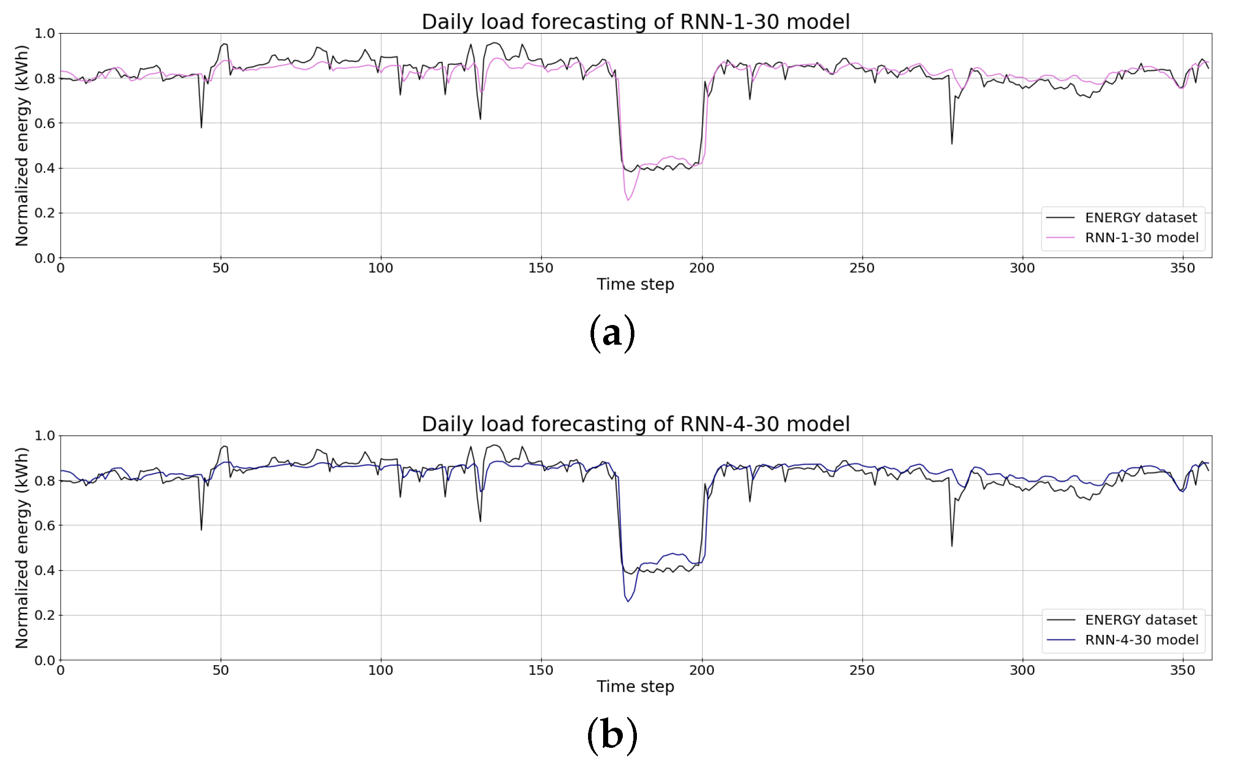
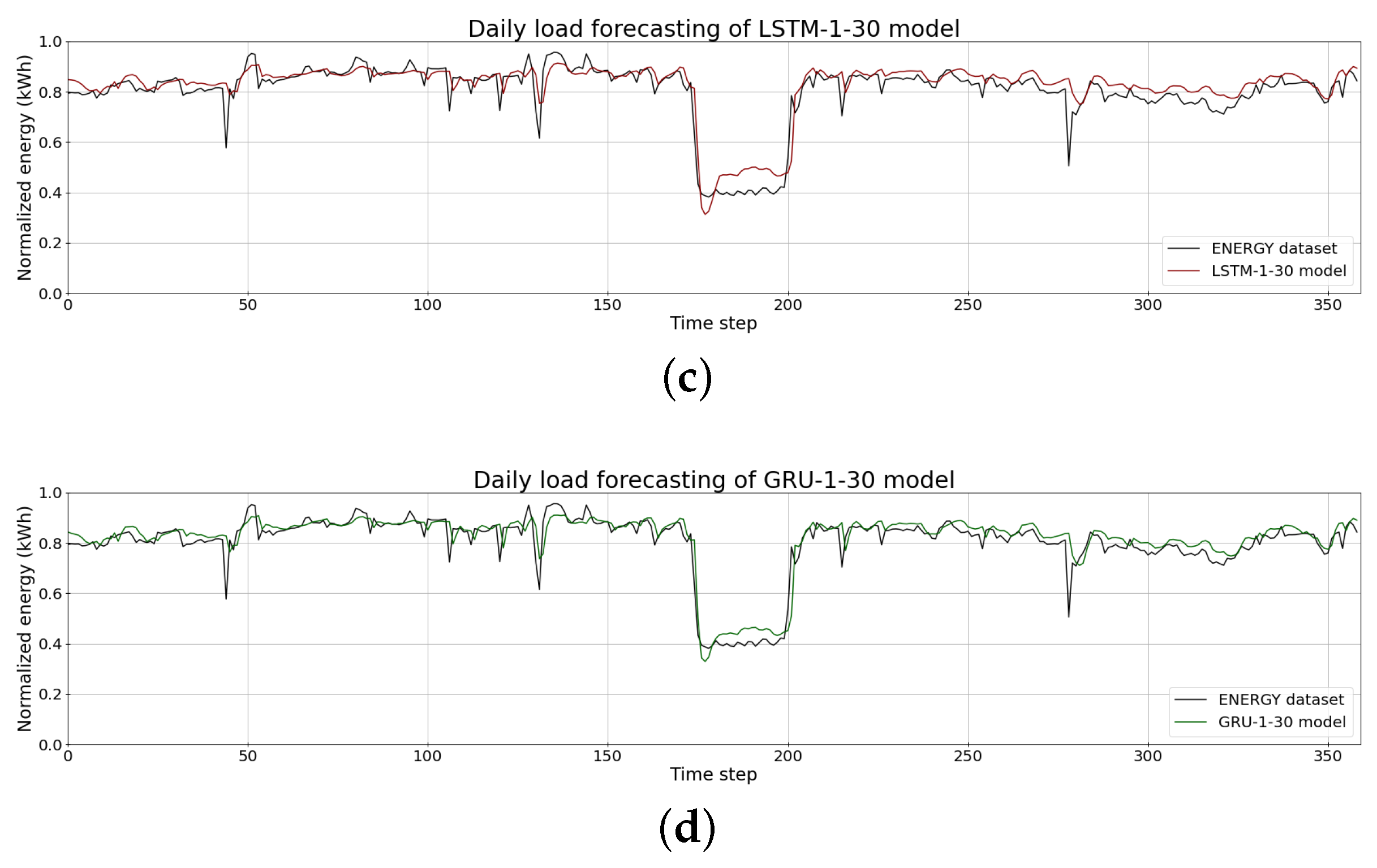
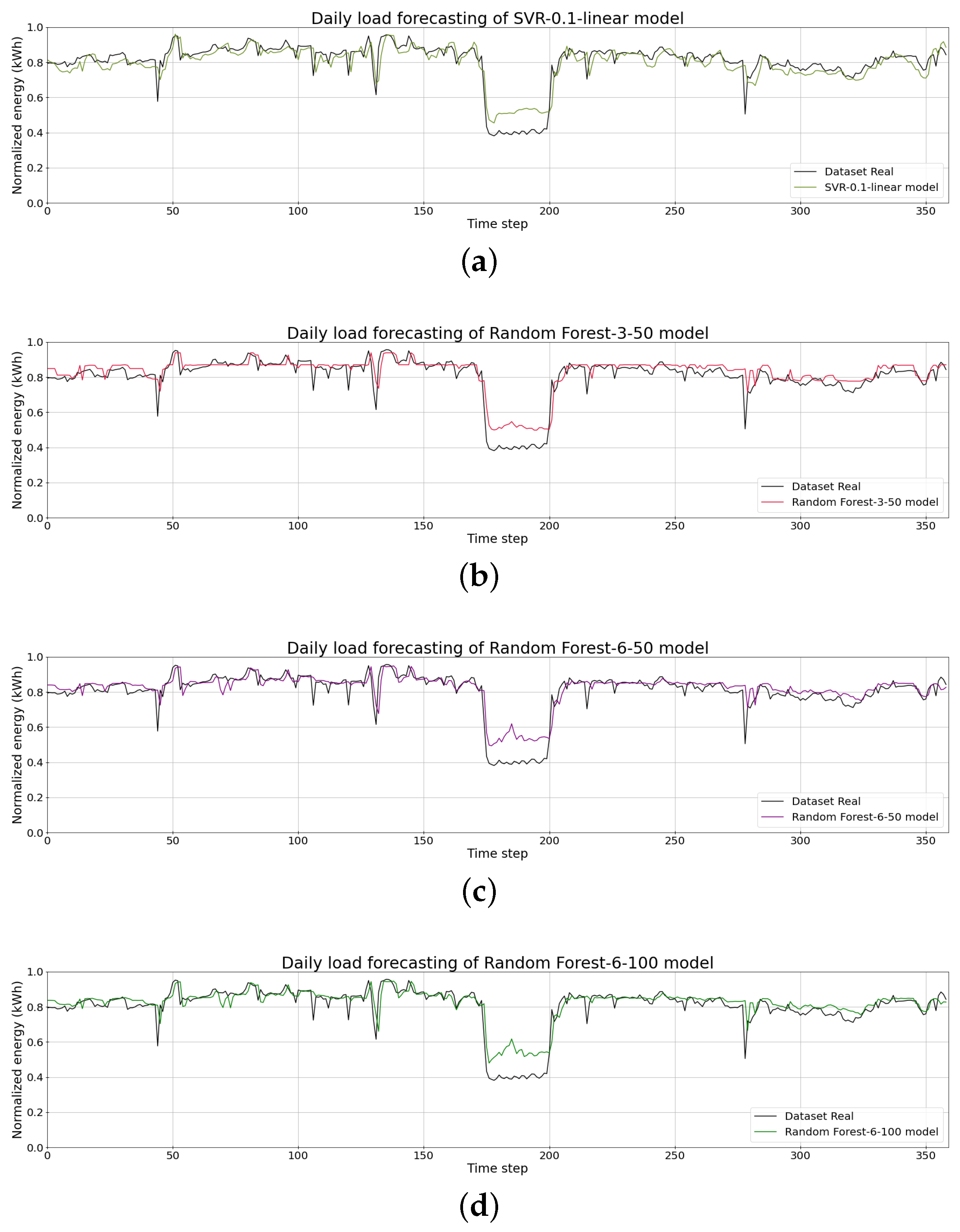
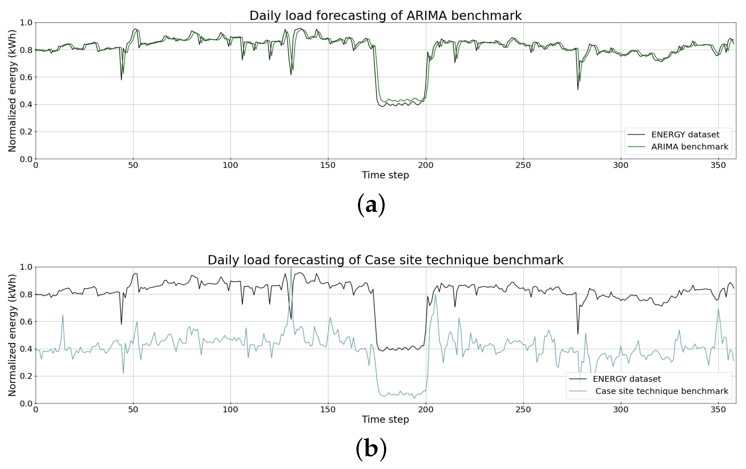
Figure 9, Figure 10 and Figure 11 illustrate the daily load forecasts for the deep-learning and machine-learning models and the manual and ARIMA benchmarks compared against the ground truth data. These clearly show that the proposed deep-learning models (Figure 9a–d) are very similar to the ground truth data compared to the existing manual technique used at the case site (Figure 11b).

Diebold–Mariano Statistical Test

Table 3 suggests that GRU-1-30 and ARIMA achieved the best results for the RMSE, MAPE, and MAE metrics. As the values of RMSE, MAPE, and MAE are very similar, we used the Diebold-Mariano [50] test to confirm the results. The Diebold-Mariano is a hypothesis test used to compare the significance of differences in two different prediction models. Table 5 presents the results obtained.
The Diebold–Mariano test result equals zero when the techniques being tested are equal; negative values are present when the left technique obtains a better performance and vice-versa. If the absolute Diebold–Mariano results are high, the tested techniques have significantly different prediction values. The first line of Table 5 shows the comparison between the case site technique compared to all other models.
It is clear that the existing manual technique used at the case site has the worst performance in comparison to the all models examined. The high statistical values obtained for this technique confirms that it is suboptimal for STLF in this case. The only model that outperformed the ARIMA model was the GRU-1-30 model. All deep-learning models outperformed the machine-learning models. However, the variance in Diebold-Mariano values are not as significant. While the Diebold-Mariano test results for deep-learning models are similar, the GRU-1-30 model achieved the best prediction indexes when compared to all models tested. As such, the initial hypothesis from the grid search results are confirmed.
These results suggest a significant improvement in the accuracy of the STLF for this energy-intensive manufacturer. This can be used to provide more accurate energy management to meet production demands, to improve cashflow, to reduce environmental impact, and to mitigate risks associated with energy inefficiencies. Accurate STLF results can be used for anticipatory optimisation and remediation. For example, anomaly detection can be used to identify possible machine degradation or failure from anomalous loads at different stages in the manufacturing process. This would enable predictive maintenance and avoid production downtime.

5. Related Work

Short term load forecasting using deep learning and machine learning has been examined from a variety of perspectives. For example, there is a well-established literature on supply-side energy consumption and demand forecasting using deep learning from the perspective of the management and optimisation of power systems and electricity grids. These include studies using deep neural networks [6], deep belief networks [51], CNNs [52], Autoencoder and LSTM [53], SVM and Random Forest [21] amongst others. The focus of this paper is demand-side. STLF for grids and utility companies have a fundamentally different motivation and context than manufacturing firms, not least the public interest aspect of energy systems, as opposed to profit maximisation, operational efficiencies and other business objectives.
Similarly, there has been a number of studies on the use of deep learning for forecasting load prediction for different energy consumer types—residential [19,22,54], commercial [55,56], and industrial [11,57]. While there are certainly new knowledge generated by these works, their focus is overwhelmingly on load forecasting for utility companies and grids. Residential and commercial use cases have fundamentally different energy consumption patterns than industry in terms of decision-making time horizon, building code standards, population density, building design, and response to regional climate, amongst others [58]. As discussed in Section 1, energy-intensive manufacturing has a significantly different energy consumption profile than other industry sectors, leaving aside the obvious differences with residential and commercial use. As a result, the motivation for load forecasting is substantially different than other industrial use cases. In particular, these operations tend to have high process-related energy requirements, are not subject to climate changes, and energy management is core capability in their business. As production is central to manufacturing, the demand for energy is derived from production planning and energy forecasting and optimisation based on the over-riding demands of production [59].
Ryu et al. [6] explore demand-side STLF for variety of industry categories including manufacturing. Using data sourced from a Korean utility company, they propose a deep neural network (DNN) based STLF framework based on industry category, temporal patterns, location and weather conditions. A comparative analysis was performed with three different forecasting techniques—shallow neural network (SNN), double seasonal Holt–Winters (DSHW) and ARIMA. Using MAPE and relative root mean squared error (RRMSE). The results suggest that the DNN-based STLF model achieved the best performance when compared to the other models with lower MAPE (2.19%) and lower RRMSE (2.76%). Our approach differs in three important ways. Firstly, we adopt RNNs that have significant advantages in terms of time series data. Second, in [6], because the data comes from the power company, all energy consumption at a firm level is bundled up and it is not possible to distinguish different sources of energy consumption and their impact from within the firm e.g., buildings vs. process-related consumption. Third, we focus on energy-intensive manufacturing. It is not clear whether energy-intensive manufacturing is included in [6].
Mawson & Hughes [60] explore the use of a deep feedforward neural networks (DFNN) and a deep RNN (DRNN) to predict STLF for a medium-sized manufacturing facility. Inputs to the DNNs included weather conditions and machining schedules. Results suggest that both models performed well but that the DRNN outperformed the DFNN for predictions of building energy consumption, achieving an accuracy of 96.8% compared to 92.4% for DFNN. The focus of [60] was optimising heating, ventilation and air conditioning (HVAC). As such, the impact of the production process was not a focus per se. While data for boiler energy, cooling energy and machine scheduling were taken in to account, again, unlike our work, specific process-related energy consumption was not considered and the focus was not energy-intensive manufacturing. Additionally, Mawson & Hughes [60] use simulated data whereas we use ground truth data to train and validate the models.
In contrast to [6,60], Chen et al. [7] study the use of DNN for STLF in an energy-intensive manufacturing use case. Using data from the melt shop of steel plant, they sought to use DNN to predict energy consumption for one specific process, the electric arc furnace (EAF) for different types of scrap. The performance of the DNN was compared with linear regression (LR), SVM, and decision tree (DT) based on the model correlation coefficient and MAE. The proposed DNN outperformed other models with the highest correlation index, at 0.854, and the lowest MAE, at 1.5%. While [7] is the closest use case to our paper, it focuses exclusively on one process and does not seek to calculate the overall plant energy consumption. While they identify the potential of deep learning over traditional statistical and machine learning approaches, they do not evaluate the relative performance against other deep learning architectures.
Yeom & Choi [15] describe a platform, E-IoT, for collecting a wide range of data (over 1556 variables for one process) at a Korean manufacturing plant. From the data collected by E-IoT, they use a least absolute shrinkage and selection operator (LASSO) technique, based on machine learning, to extract relevant variables to predict plant-level STLF based on the first stage of one process, using LSTM. The proposed LSTM model achieved an MAE of 0.07 and an accuracy of 79%. The paper suffers from a significant lack of detail. For example, while the energy consumption profile for the process presented in [15] appears energy-intensive when compared to total plant energy consumption, it is unclear from the paper whether the manufacturing plant was energy-intensive or not. It is also unclear why only the first stage of the manufacturing process was used, and how many other processes are involved. Furthermore, no detail is provided on how the LSTM model configuration was selected, and it is not compared with existing techniques or other deep learning models.
Li et al. [21] explore STLF for industrial customers in China and source data from a cable factory and a lithium factory located in Chongqing. They propose two short-term (20 days) energy consumption forecasting models using SVM and Random Forest based on historical consumption data as well as seasonal factors (holidays) and upstream value chain data i.e. the price of non-ferrous metals and raw material consumption at each factory. Both models accurately predicted the electricity loads for both factories. The MAPE for both the SVM and Random Forest model were similar for each factory - 5% for the cable factory and 2% for the lithium factory. The study highlighted the need for research using additional industry- and firm-specific variables to increase accuracy.
As can be seen from the above, there is a paucity of research on demand-side STLF for energy-intensive manufacturing using deep learning and machine learning models. Decision making for utility companies has little in common with manufacturers. Similarly, STLF for residential and commercial use has little relevance to industrial use cases, and within industrial energy consumption, energy intensive manufacturing is idiosyncratic. The few similar studies lack detail on the degree to which they are energy-intensive manufacturers, aggregate all energy consumption, or focus on one process alone. Furthermore, where proposed deep learning and machine learning models were compared, they were either evaluated against only traditional techniques or only other deep learning models, or not at all. We addressed all of these shortcomings in our paper.

6. Conclusions and Future Work

This paper is one of the first papers to compare the efficacy of deep-learning and machine-learning models for short-term load forecasting for energy-intensive manufacturing plants. In addition, we benchmark these models against the incumbent manual prediction technique and a classic time-series forecasting technique, ARIMA. Unlike existing studies, we consider multi-year ground truth data including total plant energy consumption data and data from two stages in a complex energy intensive manufacturing process. The use of production data contributed significantly to improving STLF accuracy by reducing the RMSE.
Based on both the grid search results and Diebold–Mariano test results, we found that all the deep-learning and machine-learning models outperformed the incumbent manual technique. Furthermore, the GRU model (GRU-1-30) outperformed the basic RNN and LSTM models in RMSE (0.0305), MAPE (4.33%), and MAE (0.0305) in a very short inference time (0.7058 s).
Accurate STLF can be used in a variety manufacturing processes to achieve energy efficiencies and can be used as an input in a range of operational decisions including energy management (e.g., heat storage and cooling), anomaly detection, predictive machine maintenance, and proactive plant and machine management, amongst others. The reduction of machine idle-times would seem to be particularly attractive to such manufacturers. Given the dearth of research on this topic in energy-intensive manufacturing, there are many avenues for future research. As the industrial Internet of things matures, a significantly larger volume of time-series data will be available to further refine the accuracy of the models and to extend the use of deep learning beyond prediction to actuation.
For near real-time prediction, very short-term load forecasting (VSTLF) may be needed. In such use cases, rapid training times will be required. While GRUs may meet this criteria, further research is required. Furthermore, medium-term load forecasting may prove that fruitful, deep-learning training models may need to be augmented with historic trend data to account for longer seasonal cycles or predictable events. Medium-term load forecasting may enable new use cases including switches to more sustainable or lower-cost power supplies. Similarly, as production planning is prioritised over energy management in energy-intensive manufacturing, multi-step forecasting strategy may be more appropriate or preferable. This may require ensemble solutions and is worthy of exploration.
This paper highlights the potential of deep learning and ARIMA in energy-intensive manufacturing. The adoption of deep learning, like all data science technologies, requires overcoming human, organisational, and technological challenges; however, against intense rivalry, firms may not have a choice.

Author Contributions

Conceptualization, A.M.N.C.R. and P.T.E.; data curation, A.M.N.C.R. and P.R.X.d.C.; Formal analysis, A.M.N.C.R., I.R.R., T.L. and P.T.E.; investigation, A.M.N.C.R., P.R.X.d.C., I.R.R. and P.T.E.; methodology, P.T.E.; project administration, D.S.; resources, T.L.; validation, A.M.N.C.R.; writing—original draft, A.M.N.C.R., T.L. and P.T.E.; writing—review & editing, A.M.N.C.R., D.S., T.L. and P.T.E. All authors have read and agreed to the published version of the manuscript.

Funding

This research has been partially financially supported by Fundação de Amaparo à Ciência e Tecnologia de Pernambuco (FACEPE), by the Irish Institute of Digital Business (IIDB) and dotLAB Brazil.

Conflicts of Interest

The authors declare no conflict of interest.

Abbreviations

The following abbreviations were used in this manuscript:
ANNArtificial Neural Networks
ARIMAAutoregressive Integrated Moving Average
BtuBritish Thermal Units
CNNConvolutional Neural Network
CO2Carbon Dioxide
DFNNDeep Feed Forward Neural Networks
DNNDeep Neural Network
DRNNDeep Recurrent Neural Networks
DSHWDouble Seasonal Holt–Winters
DTDecision Tree
EAFElectric Arc Furnace
GRUGated Recurrent Unit
HVACHeating, Ventilation, and Air Conditioning
LASSOLeast Absolute Shrinkage and Selection Operator
LRLinear Regression
LSTMLong Short-Term Memory
MAEMean Absolute Error
MAPEMean Absolute Percent Error
MLPMulti-Layer Perceptrons
MSEMean Squared Error
POLYPolymerization
RMSERoot Mean Squared Error
RNNRecurrent Neural Networks
RRMSERelative Root Mean Square Error
SDGSustainable Development Goals
SNNShallow Neural Network
SSPOLYSolid-State Polymerization
STLFShort-Term Load Forecasting
SVMSupport Vector Machines
SVRSupport Vector Machine Regression
TECITechnical Energy Consumption Index
VSTLFVery Short-Term Load Forecasting

References

  1. EIA. International Energy Outlook 2019. Available online: https://www.eia.gov/outlooks/ieo/ (accessed on 24 April 2020).
  2. EIA. International Energy Outlook 2016 with Projections to 2040; Government Printing Office: Washington, DC, USA, 2016.
  3. Gozgor, G.; Lau, C.K.M.; Lu, Z. Energy consumption and economic growth: New evidence from the OECD countries. Energy 2018, 153, 27–34. [Google Scholar] [CrossRef] [Green Version]
  4. SDG. Build Resilient Infrastructure, Promote Inclusive and Sustainable Industrialization and Foster Innovation. Available online: https://sustainabledevelopment.un.org/sdg9 (accessed on 24 April 2020).
  5. Sundarakani, B.; De Souza, R.; Goh, M.; Wagner, S.M.; Manikandan, S. Modeling carbon footprints across the supply chain. Int. J. Prod. Econ. 2010, 128, 43–50. [Google Scholar] [CrossRef]
  6. Ryu, S.; Noh, J.; Kim, H. Deep neural network based demand side short term load forecasting. Energies 2017, 10, 3. [Google Scholar] [CrossRef]
  7. Chen, C.; Liu, Y.; Kumar, M.; Qin, J. Energy consumption modelling using deep learning technique—A case study of EAF. Procedia CIRP 2018, 72, 1063–1068. [Google Scholar] [CrossRef]
  8. Demirhan, H.; Renwick, Z. Missing value imputation for short to mid-term horizontal solar irradiance data. Appl. Energy 2018, 225, 998–1012. [Google Scholar] [CrossRef]
  9. Andiojaya, A.; Demirhan, H. A bagging algorithm for the imputation of missing values in time series. Expert Syst. Appl. 2019, 129, 10–26. [Google Scholar] [CrossRef]
  10. Peppanen, J.; Zhang, X.; Grijalva, S.; Reno, M.J. Handling bad or missing smart meter data through advanced data imputation. In Proceedings of the 2016 IEEE Power & Energy Society Innovative Smart Grid Technologies Conference (ISGT), Minneapolis, MN, USA, 6–9 September 2016; pp. 1–5. [Google Scholar]
  11. Azadeh, A.; Ghaderi, S.; Sohrabkhani, S. Annual electricity consumption forecasting by neural network in high energy consuming industrial sectors. Energy Convers. Manag. 2008, 49, 2272–2278. [Google Scholar] [CrossRef]
  12. Berriel, R.F.; Lopes, A.T.; Rodrigues, A.; Varejao, F.M.; Oliveira-Santos, T. Monthly energy consumption forecast: A deep learning approach. In Proceedings of the 2017 International Joint Conference on Neural Networks (IJCNN), Anchorage, AK, USA, 14–19 May 2017; pp. 4283–4290. [Google Scholar]
  13. Kuo, P.H.; Huang, C.J. A high precision artificial neural networks model for short-term energy load forecasting. Energies 2018, 11, 213. [Google Scholar] [CrossRef] [Green Version]
  14. Debnath, K.B.; Mourshed, M. Forecasting methods in energy planning models. Renew. Sustain. Energy Rev. 2018, 88, 297–325. [Google Scholar] [CrossRef] [Green Version]
  15. Yeom, K.R.; Choi, H.S. Prediction of Manufacturing Plant’s Electric Power Using Machine Learning. In Proceedings of the 2018 Tenth International Conference on Ubiquitous and Future Networks (ICUFN), Prague, Czech Republic, 3–6 July 2018; pp. 814–816. [Google Scholar]
  16. Willmott, C.J.; Matsuura, K. Advantages of the mean absolute error (MAE) over the root mean square error (RMSE) in assessing average model performance. Clim. Res. 2005, 30, 79–82. [Google Scholar] [CrossRef]
  17. Hsieh, T.J.; Hsiao, H.F.; Yeh, W.C. Forecasting stock markets using wavelet transforms and recurrent neural networks: An integrated system based on artificial bee colony algorithm. Appl. Soft Comput. 2011, 11, 2510–2525. [Google Scholar] [CrossRef]
  18. Kolomvatsos, K.; Papadopoulou, P.; Anagnostopoulos, C.; Hadjiefthymiades, S. A Spatio-Temporal Data Imputation Model for Supporting Analytics at the Edge. In Proceedings of the Conference on e-Business, e-Services and e-Society, Trondheim, Norway, 18–20 September 2019; pp. 138–150. [Google Scholar]
  19. Kong, W.; Dong, Z.Y.; Jia, Y.; Hill, D.J.; Xu, Y.; Zhang, Y. Short-term residential load forecasting based on LSTM recurrent neural network. IEEE Trans. Smart Grid 2017, 10, 841–851. [Google Scholar] [CrossRef]
  20. De Myttenaere, A.; Golden, B.; Le Grand, B.; Rossi, F. Mean absolute percentage error for regression models. Neurocomputing 2016, 192, 38–48. [Google Scholar] [CrossRef] [Green Version]
  21. Li, Q.; Zhang, L.; Xiang, F. Short-term Load Forecasting: A Case Study in Chongqing Factories. In Proceedings of the 2019 6th International Conference on Information Science and Control Engineering (ICISCE), Shanghai, China, 20–22 December 2019; pp. 892–897. [Google Scholar]
  22. Güngör, O.; Akşanlı, B.; Aydoğan, R. Algorithm selection and combining multiple learners for residential energy prediction. Future Gener. Comput. Syst. 2019, 99, 391–400. [Google Scholar] [CrossRef]
  23. Lago, J.; De Ridder, F.; De Schutter, B. Forecasting spot electricity prices: Deep learning approaches and empirical comparison of traditional algorithms. Appl. Energy 2018, 221, 386–405. [Google Scholar] [CrossRef]
  24. Bengio, Y.; Simard, P.; Frasconi, P. Learning long-term dependencies with gradient descent is difficult. IEEE Trans. Neural Netw. 1994, 5, 157–166. [Google Scholar] [CrossRef] [PubMed]
  25. Chung, J.; Gulcehre, C.; Cho, K.; Bengio, Y. Empirical evaluation of gated recurrent neural networks on sequence modeling. arXiv 2014, arXiv:1412.3555. [Google Scholar]
  26. Sundermeyer, M.; Schlüter, R.; Ney, H. LSTM neural networks for language modeling. In Proceedings of the Thirteenth Annual Conference of the International Speech Communication Association, Oregon, Portland, 9–13 September 2012. [Google Scholar]
  27. Hochreiter, S.; Schmidhuber, J. Long short-term memory. Neural Comput. 1997, 9, 1735–1780. [Google Scholar] [CrossRef]
  28. Gers, F.A.; Schmidhuber, J.; Cummins, F. Learning to forget: Continual prediction with LSTM. In Proceedings of the 1999 Ninth International Conference on Artificial Neural Networks ICANN 99. (Conf. Publ. No. 470), Edinburgh, UK, 7–10 September 1999; Volume 2, pp. 850–855. [Google Scholar] [CrossRef]
  29. Jozefowicz, R.; Zaremba, W.; Sutskever, I. An empirical exploration of recurrent network architectures. In Proceedings of the International Conference on Machine Learning, Lille, France, 6–11 July 2015; pp. 2342–2350. [Google Scholar]
  30. Bergstra, J.; Bengio, Y. Random search for hyper-parameter optimization. J. Mach. Learn. Res. 2012, 13, 281–305. [Google Scholar]
  31. Liao, J.M.; Chang, M.J.; Chang, L.M. Prediction of Air-Conditioning Energy Consumption in R&D Building Using Multiple Machine Learning Techniques. Energies 2020, 13, 1847. [Google Scholar]
  32. Yoon, H.; Kim, Y.; Ha, K.; Lee, S.H.; Kim, G.P. Comparative evaluation of ANN-and SVM-time series models for predicting freshwater-saltwater interface fluctuations. Water 2017, 9, 323. [Google Scholar] [CrossRef] [Green Version]
  33. Kavaklioglu, K. Modeling and prediction of Turkey’s electricity consumption using Support Vector Regression. Appl. Energy 2011, 88, 368–375. [Google Scholar] [CrossRef]
  34. Samsudin, R.; Shabri, A.; Saad, P. A comparison of time series forecasting using support vector machine and artificial neural network model. J. Appl. Sci. 2010, 10, 950–958. [Google Scholar] [CrossRef] [Green Version]
  35. Young, S.R.; Rose, D.C.; Karnowski, T.P.; Lim, S.H.; Patton, R.M. Optimizing deep learning hyper-parameters through an evolutionary algorithm. In Proceedings of the Workshop on Machine Learning in High-Performance Computing Environments, Austin, TX, USA, 15 November 2015; pp. 1–5. [Google Scholar]
  36. Han, J.; Moraga, C. The influence of the sigmoid function parameters on the speed of backpropagation learning. In From Natural to Artificial Neural Computation; Mira, J., Sandoval, F., Eds.; Springer: Berlin/Heidelberg, Germany, 1995; pp. 195–201. [Google Scholar]
  37. Sapankevych, N.I.; Sankar, R. Time series prediction using support vector machines: A survey. IEEE Comput. Intell. Mag. 2009, 4, 24–38. [Google Scholar] [CrossRef]
  38. Vapnik, V. The Nature of Statistical Learning Theory (p. 189); Springer: New York, NY, USA, 1995; Volume 10, p. 978. [Google Scholar]
  39. Müller, K.R.; Smola, A.J.; Rätsch, G.; Schölkopf, B.; Kohlmorgen, J.; Vapnik, V. Predicting time series with support vector machines. In Proceedings of the International Conference on Artificial Neural Networks, Lausanne, Switzerland, 8–10 October 1997; pp. 999–1004. [Google Scholar]
  40. Simon, H. Neural Networks: A Comprehensive Foundation; Prentice Hall Inc.: Upper Saddle River, NJ, USA, 1999. [Google Scholar]
  41. Drucker, H.; Burges, C.J.; Kaufman, L.; Smola, A.J.; Vapnik, V. Support vector regression machines. In Proceedings of the Advances in Neural Information Processing Systems, Denver, CO, USA, 1–6 December 1997; pp. 155–161. [Google Scholar]
  42. Golkarnarenji, G.; Naebe, M.; Badii, K.; Milani, A.S.; Jazar, R.N.; Khayyam, H. Support vector regression modelling and optimization of energy consumption in carbon fiber production line. Comput. Chem. Eng. 2018, 109, 276–288. [Google Scholar] [CrossRef]
  43. Breiman, L. Random forests. Mach. Learn. 2001, 45, 5–32. [Google Scholar] [CrossRef] [Green Version]
  44. Cutler, D.R.; Edwards, T.C., Jr.; Beard, K.H.; Cutler, A.; Hess, K.T.; Gibson, J.; Lawler, J.J. Random forests for classification in ecology. Ecology 2007, 88, 2783–2792. [Google Scholar] [CrossRef]
  45. Liaw, A.; Wiener, M. Classification and regression by randomForest. R News 2002, 2, 18–22. [Google Scholar]
  46. Lahouar, A.; Slama, J.B.H. Day-ahead load forecast using random forest and expert input selection. Energy Convers. Manag. 2015, 103, 1040–1051. [Google Scholar] [CrossRef]
  47. Li, C.; Tao, Y.; Ao, W.; Yang, S.; Bai, Y. Improving forecasting accuracy of daily enterprise electricity consumption using a random forest based on ensemble empirical mode decomposition. Energy 2018, 165, 1220–1227. [Google Scholar] [CrossRef]
  48. Caruana, R.; Karampatziakis, N.; Yessenalina, A. An empirical evaluation of supervised learning in high dimensions. In Proceedings of the 25th International Conference on Machine Learning, Helsinki, Finland, 5–9 July 2008; pp. 96–103. [Google Scholar]
  49. Pushp, S. Merging Two Arima Models for Energy Optimization in WSN. arXiv 2010, arXiv:1006.5436. [Google Scholar]
  50. Diebold, F.X. Comparing predictive accuracy, twenty years later: A personal perspective on the use and abuse of Diebold—Mariano tests. J. Bus. Econ. Stat. 2015, 33, 1. [Google Scholar] [CrossRef] [Green Version]
  51. Qiu, X.; Ren, Y.; Suganthan, P.N.; Amaratunga, G.A. Empirical mode decomposition based ensemble deep learning for load demand time series forecasting. Appl. Soft Comput. 2017, 54, 246–255. [Google Scholar] [CrossRef]
  52. Dong, X.; Qian, L.; Huang, L. Short-term load forecasting in smart grid: A combined CNN and K-means clustering approach. In Proceedings of the 2017 IEEE International Conference on Big Data and Smart Computing (BigComp), Jeju, Korea, 13–16 February 2017; pp. 119–125. [Google Scholar]
  53. Gensler, A.; Henze, J.; Sick, B.; Raabe, N. Deep Learning for solar power forecasting—An approach using AutoEncoder and LSTM Neural Networks. In Proceedings of the 2016 IEEE International Conference on Systems, Man, and Cybernetics (SMC), Budapest, Hungary, 9–12 October 2016; pp. 002858–002865. [Google Scholar]
  54. Shi, H.; Xu, M.; Li, R. Deep learning for household load forecasting—A novel pooling deep RNN. IEEE Trans. Smart Grid 2017, 9, 5271–5280. [Google Scholar] [CrossRef]
  55. Xypolytou, E.; Meisel, M.; Sauter, T. Short-term electricity consumption forecast with artificial neural networks—A case study of office buildings. In Proceedings of the 2017 IEEE Manchester PowerTech, Manchester, UK, 18–22 June 2017; pp. 1–6. [Google Scholar]
  56. Petri, I.; Li, H.; Rezgui, Y.; Chunfeng, Y.; Yuce, B.; Jayan, B. Deep learning for household load forecasting—A novel pooling deep RNN. Renew. Sustain. Energy Rev. 2014, 38, 990–1002. [Google Scholar] [CrossRef]
  57. Olanrewaju, O.A. Predicting Industrial Sector’s Energy Consumption: Application of Support Vector Machine. In Proceedings of the 2019 IEEE International Conference on Industrial Engineering and Engineering Management (IEEM), Macao, China, 15–18 December 2019; pp. 1597–1600. [Google Scholar]
  58. Hobby, J.D.; Tucci, G.H. Analysis of the residential, commercial and industrial electricity consumption. In Proceedings of the 2011 IEEE PES Innovative Smart Grid Technologies (ISGT), Perth, WA, Australia, 13–16 November 2011; pp. 1–7. [Google Scholar]
  59. Hadera, H.; Labrik, R.; Mäntysaari, J.; Sand, G.; Harjunkoski, I.; Engell, S. Integration of energy-cost optimization and production scheduling using multiparametric programming. Comput. Aided Chem. Eng. 2016, 38, 559–564. [Google Scholar]
  60. Mawson, V.J.; Hughes, B.R. Deep Learning techniques for energy forecasting and condition monitoring in the manufacturing sector. Energy Build. 2020, 217, 109966. [Google Scholar] [CrossRef]
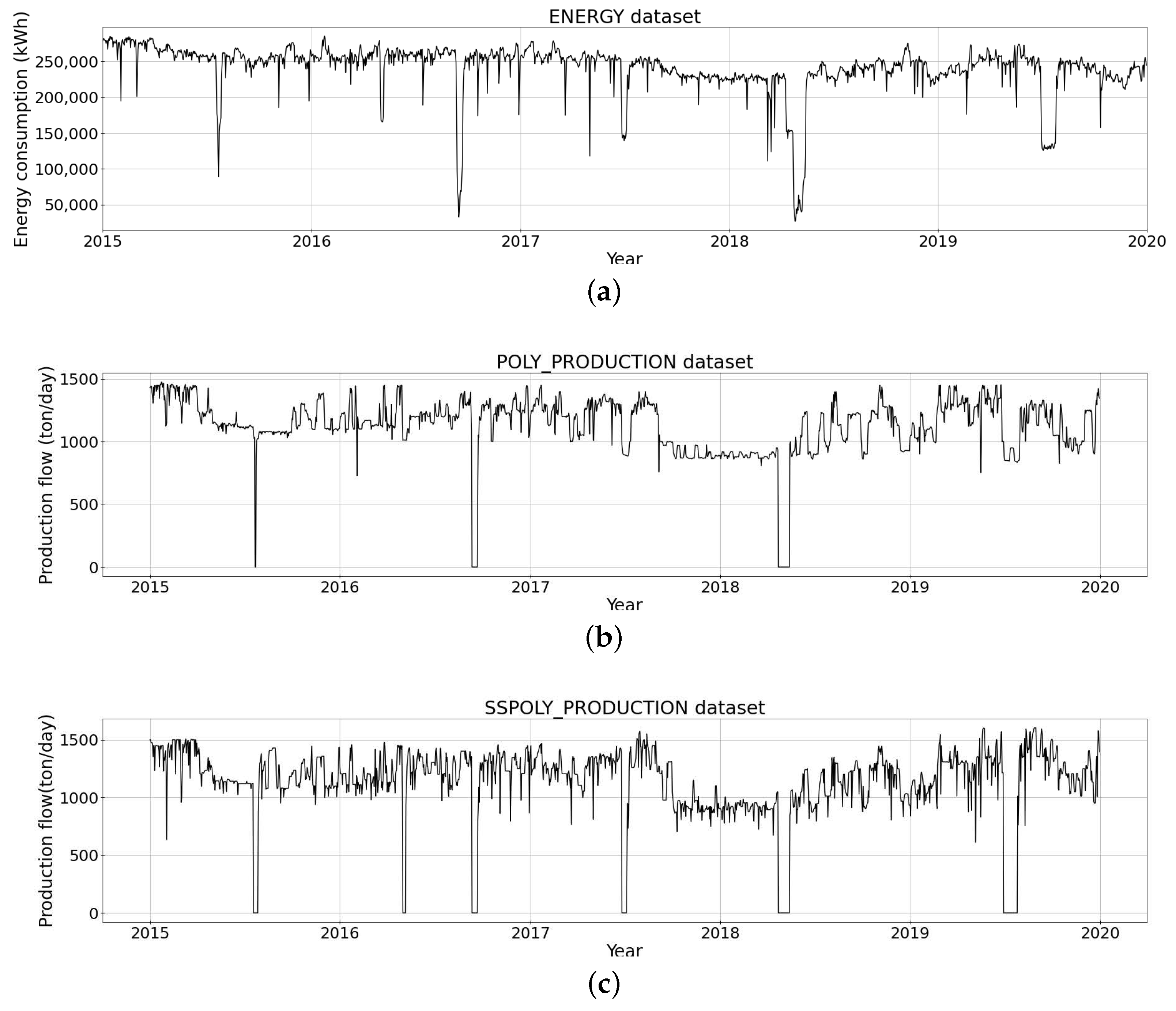
Figure 1. Daily dataset of (a) the energy consumption, (b) the production flow for the polymerisation stage, and (c) the production flow for the solid-state polymerisation stage.
Algorithms 13 00274 g001
Figure 2. Convergence results for (a) Recurrent Neural Network (RNN)-1-30, (b) RNN-4-30, (c) Long Short-Term Memory (LSTM)-1-30, and (d) Gated Recurrent Unit (GRU)-1-30.
Algorithms 13 00274 g002
Figure 3. Root mean squared error (RMSE) grid search result for (a) simple RNN, (b) LSTM, and (c) GRU.
Algorithms 13 00274 g003
Figure 4. Mean absolute percent error (MAPE) grid search result for (a) simple RNN, (b) LSTM, and (c) GRU.
Algorithms 13 00274 g004
Figure 5. Mean absolute error (MAE) grid search result for (a) simple RNN, (b) LSTM, and (c) GRU.
Algorithms 13 00274 g005
Figure 6. RMSE grid search result for (a) SVR and (b) Random Forest.
Algorithms 13 00274 g006
Figure 7. MAPE grid search result for (a) SVR and (b) Random Forest.
Algorithms 13 00274 g007
Figure 8. MAE grid search result for (a) SVR and (b) Random Forest.
Algorithms 13 00274 g008
Figure 9. Daily load forecasting using (a) the RNN-1-30 model, (b) the RNN-4-30 model, (c) the LSTM-1-30 model, and (d) the GRU-1-30 model.
Algorithms 13 00274 g009aAlgorithms 13 00274 g009b
Figure 10. Daily load forecasting using (a) the SVR-0.1-linear model, (b) the Random Forest-3-50 model, (c) the Random Forest-6-50 model, and (d) the Random Forest-6-100 model.
Algorithms 13 00274 g010
Figure 11. Daily load forecasting using (a) the case site technique and (b) the ARIMA model.
Algorithms 13 00274 g011
Table 1. Parameter and levels of deep learning techniques.
ParameterLevels
Number of nodesFrom 10 to 90, step 20
Number of layersFrom 1 to 4, step 1
Table 2. Machine-learning parameters and levels.
TechniqueParameterLevels
SVRNumber of C0.1, 1 and 10
SVRType of kernelLinear, polinomial and RBF
Random ForestNumber of max. depthFrom 3 to 6, step 1
Random ForestNumber of treesFrom 50 to 200, step 50
Table 3. RMSE, MAPE, and MAE results for the selected analysed model.
ModelsRMSEMAPE (%)MAE
ARIMA0.04713.520.0249
RNN-1-300.03164.420.0316
RNN-4-300.03204.400.0320
LSTM-1-300.03104.370.0310
GRU-1-300.03054.330.0305
SVR-0.1-linear0.05565.090.0400
Random Forest-3-500.05614.940.0377
Random Forest-6-500.05734.820.0356
Random Forest-6-1000.05804.830.0355
Case site technique0.411951.610.4039
Table 4. Average inference times for all models.
ModelsInference Time Average
(s)
ARIMA56.3565 ± 0.6802
RNN-1-300.3896 ± 0.1289
RNN-4-300.5939 ± 0.2070
LSTM-1-300.6751 ± 0.2480
GRU-1-300.7058 ± 0.2866
SVR-0.1-linear0.0014 ± 0.0004
Random Forest-3-500.0043 ± 0.0004
Random Forest-6-500.0046 ± 0.0001
Random Forest-6-1000.0080 ± 0.0012
Table 5. Two-sample Diebold-Mariano test results for the deep-learning and machine-learning models and the manual and ARIMA approaches.
ARIMARNN-1-30RNN-4-30LSTM-1-30GRU-1-30SVR-0.1-
Linear
Random
Forest-3-50
Random
Forest-6-50
Random
Forest-6-100
Case site
technique
51.3851.5551.2750.7951.3051.0650.2049.7649.70
ARIMA-−0.54−0.83−1.460.45−2.96−3.36−2.95−3.18
RNN-1-30--−1.39−1.341.99−2.43−2.76−2.41−2.56
RNN-4-30---−0.993.04−2.07−2.57−2.25−2.40
LSTM-1-30----6.56−1.96−2.81−2.37−2.54
GRU-1-30-----−3.87−4.47−3.61−3.71
SVR-0.1-linear------−0.24−0.78−1.08
Random
Forest-3-50
-------−0.76−1.15
Random
Forest-6-50
--------−1.83
Publisher’s Note: MDPI stays neutral with regard to jurisdictional claims in published maps and institutional affiliations.