Multi-Metaheuristic Competitive Model for Optimization of Fuzzy Controllers


Abstract
1. Introduction
2. Background on FA, WDO, DSO, and Fuzzy Logic
2.1. Firefly Algorithm (FA)
2.2. Wind-Driven Optimization (WDO)
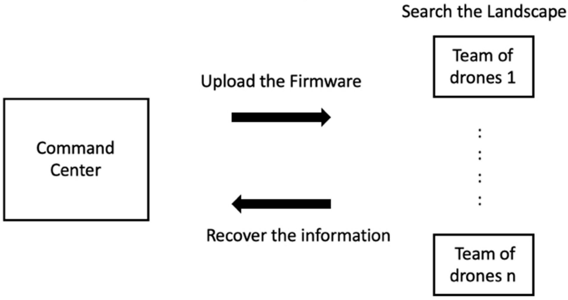
2.3. Drone Squadron Optimization (DSO)
- 1.-
- Maintain partial control of the search.
- 2.-
- Develop new control software for drones.
- Coordinates: representing a numerical solution.
- Scan the landscape: calculate the objective function and obtain the fitness value.
- Firmware: distinct rules/configurations to evolve the population.
- Team: group of agents that share a firmware, but operate on possibly different data.
- Squadron: group of teams with different firmware.
2.4. Fuzzy Logic
3. Proposed Methodology
3.1. Case 1: Benchmark Functions
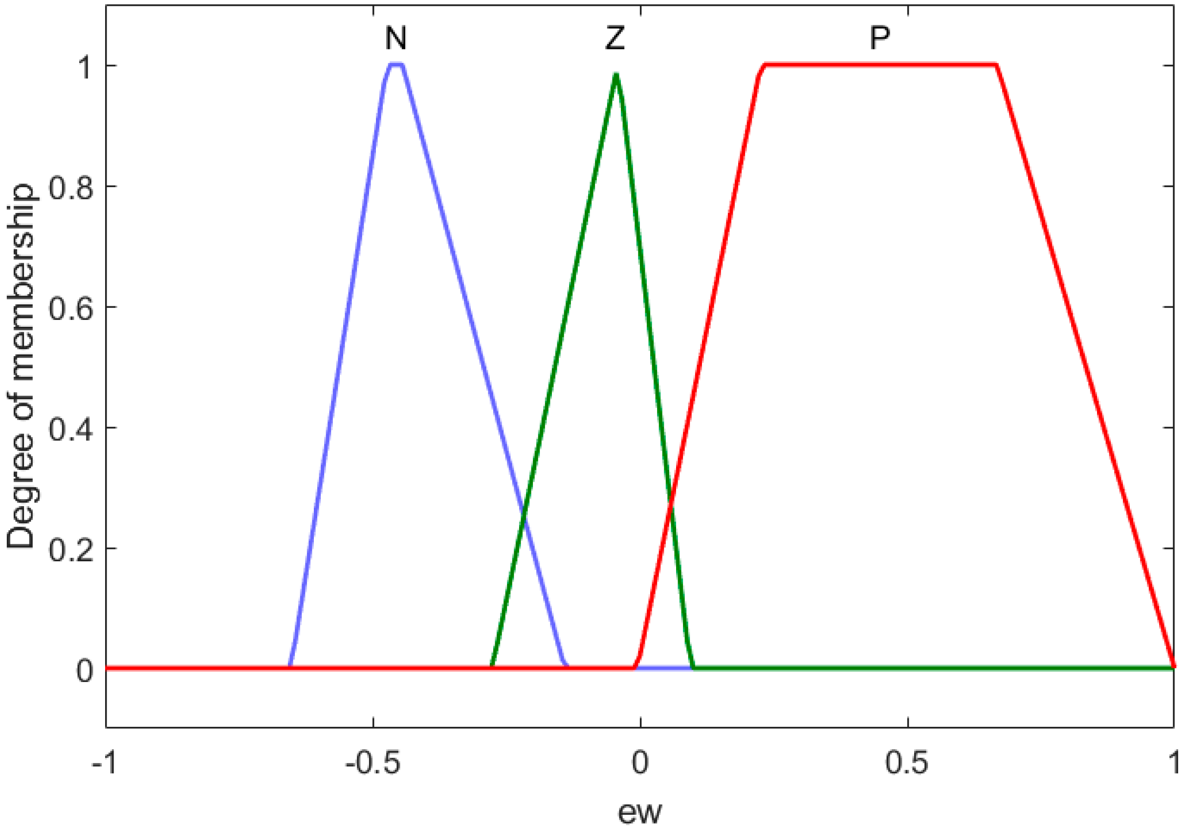
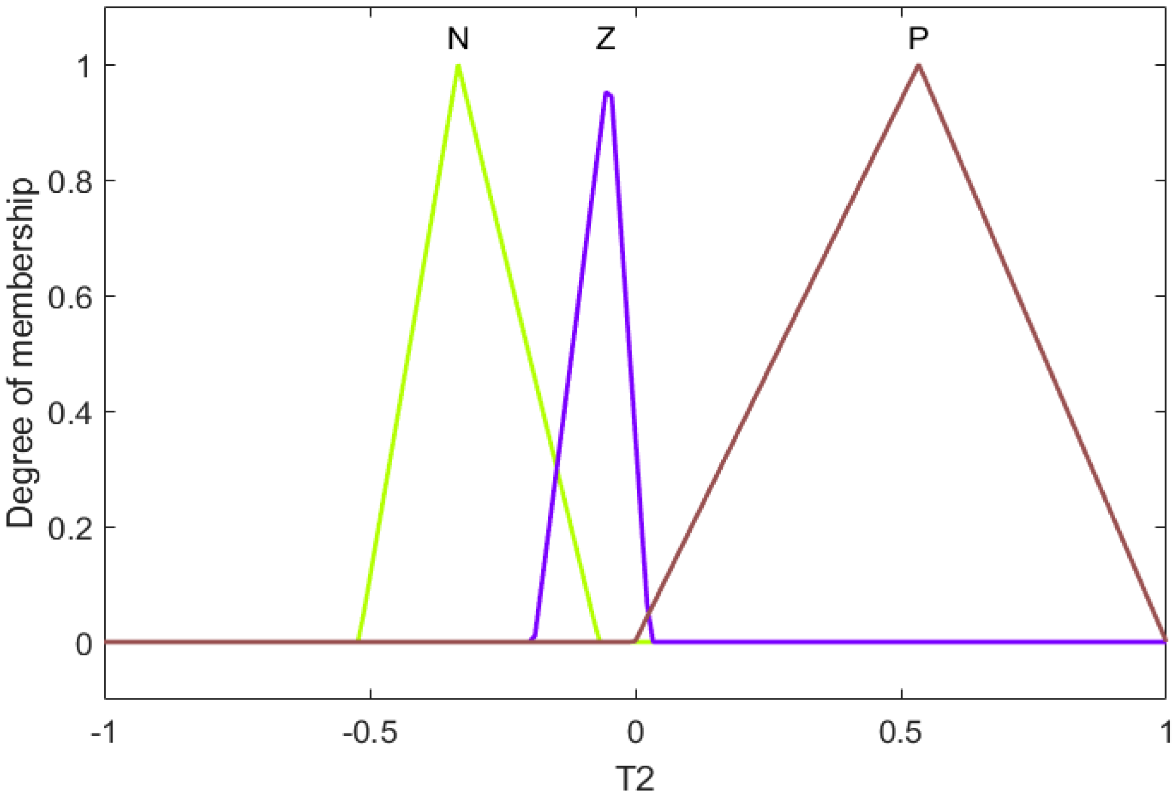
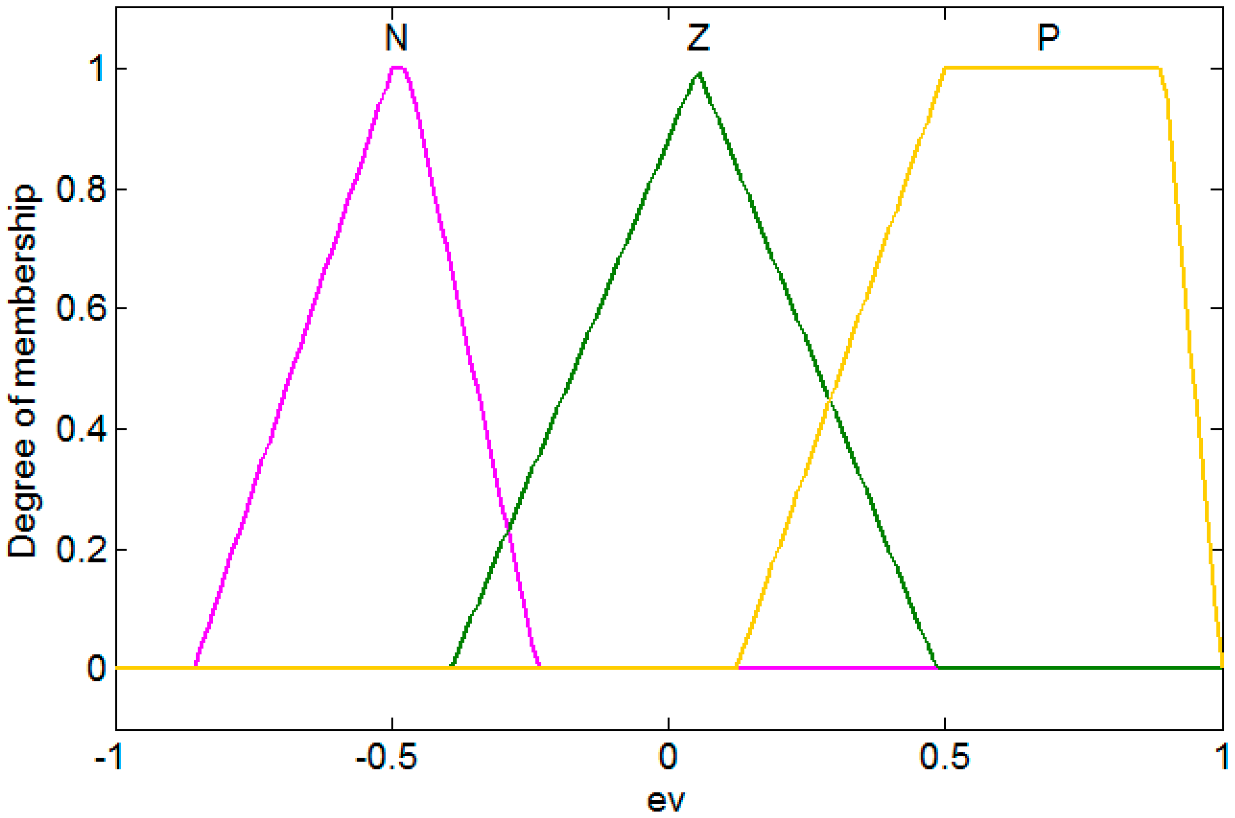
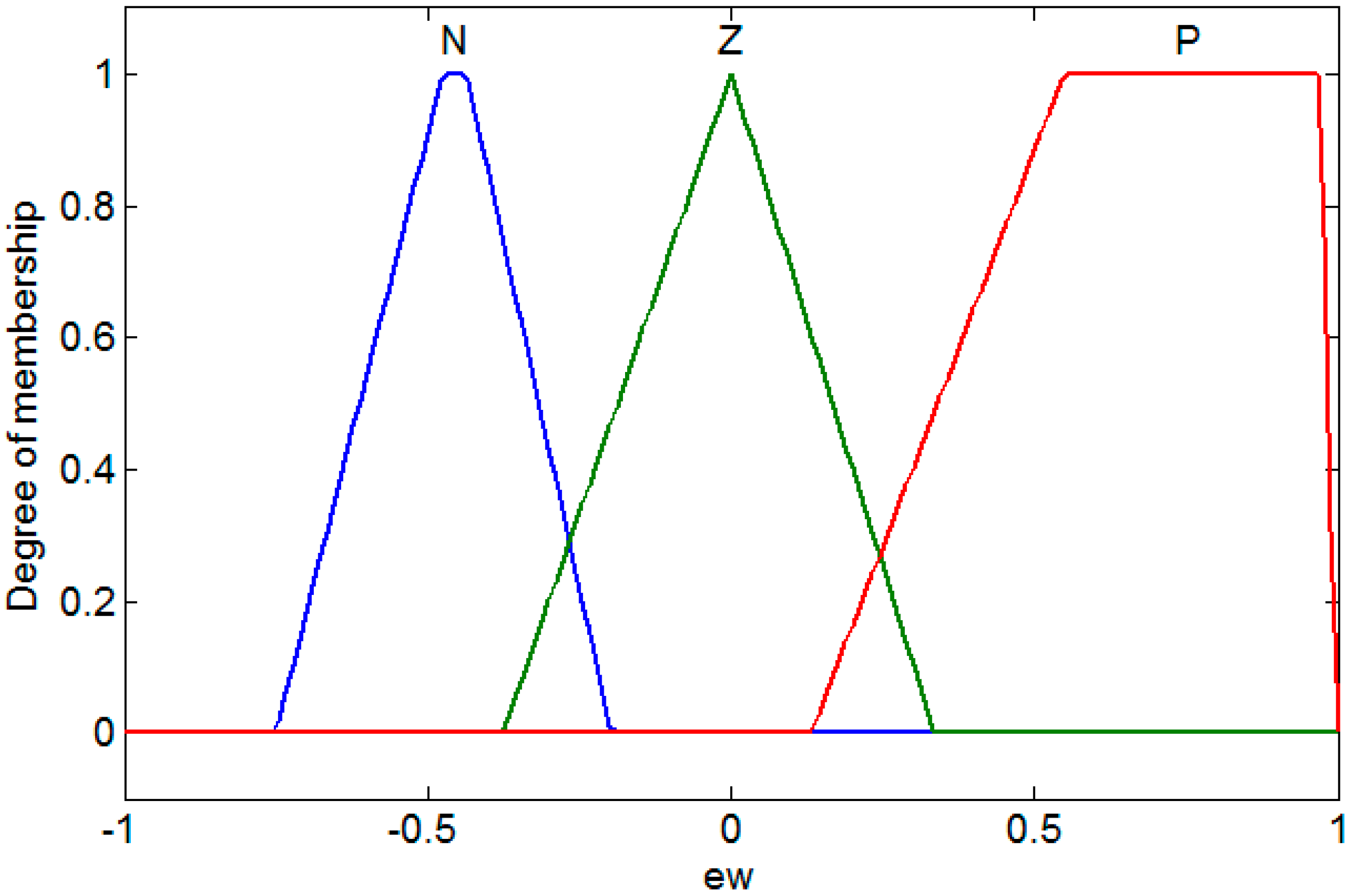
3.2. Case 2 Fuzzy Controller
4. Results
4.1. Case 1 Results: Benchmark Functions
4.2. Case 2 Results of the Fuzzy Controller Optimization
5. Discussion
6. Conclusions
Author Contributions
Funding
Acknowledgments
Conflicts of Interest
References
- Lukovac, V.; Pamučar, D.; Popović, M.; Đorović, B. Portfolio model for analyzing human resources: An approach based on neuro-fuzzy modeling and the simulated annealing algorithm. Expert Syst. Appl. 2017, 90, 318–331. [Google Scholar] [CrossRef]
- Pamučar, D.; Vasin, L.; Atanasković, P.; Miličić, M. Planning the City Logistics Terminal Location by Applying the Green p-Median Model and Type-2 Neurofuzzy Network. Comput. Intell. Neurosci. 2016, 2016, 1–15. [Google Scholar] [CrossRef]
- Sremac, S.; Tanackov, I.; Kopić, M.; Radović, D. ANFIS model for determining the economic order quantity. Decis. Mak. Appl. Manag. Eng. 2018, 2, 81–92. [Google Scholar] [CrossRef]
- Stojčić, M.; Stjepanović, A.; Stjepanović, Đ. ANFIS model for the prediction of generated electricity of photovoltaic modules. Decis. Mak. Appl. Manag. Eng. 2019, 1, 35–48. [Google Scholar] [CrossRef]
- Pamucar, D.; Ćirović, G. Vehicle route selection with an adaptive neuro fuzzy inference system in uncertainty conditions. Decis. Mak. Appl. Manag. Eng. 2018, 1, 13–37. [Google Scholar] [CrossRef]
- Pamučar, D.; Ljubojević, S.; Kostadinović, D.; Đorović, B. Cost and risk aggregation in multi-objective route planning for hazardous materials transportation—A neuro-fuzzy and artificial bee colony approach. Expert Syst. Appl. 2016, 65, 1–15. [Google Scholar] [CrossRef]
- Pamučar, D.; Atanasković, P.; Miličić, M. Modeling of fuzzy logic system for investment management in the railway infrastructure. Teh. Vjesn. Tech. Gaz. 2015, 22. [Google Scholar] [CrossRef]
- Dorigo, M.; Gambardella, L.M. Ant colony system: A cooperative learning approach to the traveling salesman problem. IEEE Trans. Evol. Comput. 1997, 1, 53–66. [Google Scholar] [CrossRef]
- Liu, J.; Yang, J.; Liu, H.; Tian, X.; Gao, M. An improved ant colony algorithm for robot path planning. Soft Comput. 2017, 21, 5829–5839. [Google Scholar] [CrossRef]
- Dorigo, M.; Birattari, M.; Blum, C.; Clerc, M.; Stutzle, T.; Winfield, A. Ant colony optimization and swarm intelligence. In Proceedings of the ANTS 2008: The 6th International Conference on Ant Colony Optimization and Swarm Intelligence, Brussels, Belgium, 22–24 September 2008; Springer: Berlin, Germany, 2008; Volume 5217. [Google Scholar]
- Holland, J.H. Adaptation in Natural and Artificial Systems: An Introductory Analysis with Applications to Biology, Control, and Artificial Intelligence; MIT Press: Cambridge, MA, USA, 1992. [Google Scholar]
- Pal, S.K.; Wang, P.P. Genetic Algorithms for Pattern Recognition; CRC Press: Boca Raton, FL, USA, 2017. [Google Scholar]
- Garg, H. A hybrid GSA-GA algorithm for constrained optimization problems. Inf. Sci. 2019, 478, 499–523. [Google Scholar] [CrossRef]
- Patwal, R.S.; Narang, N.; Garg, H. A novel TVAC-PSO based mutation strategies algorithm for generation scheduling of pumped storage hydrothermal system incorporating solar units. Energy 2018, 142, 822–837. [Google Scholar] [CrossRef]
- Garg, H. A hybrid PSO-GA algorithm for constrained optimization problems. Appl. Math. Comput. 2016, 274, 292–305. [Google Scholar] [CrossRef]
- Garg, H.; Sharma, S.P. Multi-objective reliability-redundancy allocation problem using particle swarm optimization. Comput. Ind. Eng. 2013, 61, 247–255. [Google Scholar] [CrossRef]
- Garg, H. Solving structural engineering design optimization problems using an artificial bee colony algorithm. J. Ind. Manag. Optim. 2014, 3, 777–794. [Google Scholar] [CrossRef]
- Lagunes, M.L.; Castillo, O.; Soria, J.; Garcia, M.; Valdez, F. Optimization of granulation for fuzzy controllers of autonomous mobile robots using the Firefly Algorithm. Granul. Comput. 2019, 4, 185–195. [Google Scholar] [CrossRef]
- Bernal, E.; Castillo, O.; Soria, J. Imperialist Competitive Algorithm with Dynamic Parameter Adaptation Applied to the Optimization of Mathematical Functions. In Nature-Inspired Design of Hybrid Intelligent Systems; Springer: Cham, Switzerland, 2017; Volume 667, pp. 329–341. [Google Scholar]
- Caraveo, C.; Valdez, F.; Castillo, O. A New Meta-Heuristics of Optimization with Dynamic Adaptation of Parameters Using Type-2 Fuzzy Logic for Trajectory Control of a Mobile Robot. Algorithms 2017, 10, 85. [Google Scholar] [CrossRef]
- Olivas, F.; Amador-Angulo, L.; Perez, J.; Careveo, C.; Valdez, F.; Castillo, O. Comparative Study of Type-2 Fuzzy Particle Swarm, Bee Colony and Bat Algorithms in Optimization of Fuzzy Controllers. Algorithms 2017, 10, 101. [Google Scholar] [CrossRef]
- Lagunes, M.L.; Castillo, O.; Soria, J. Methodology for the Optimization of a Fuzzy Controller Using a Bio-inspired Algorithm. In Proceedings of the North American Fuzzy Information Processing Society Annual Conference, Cancun, Mexico, 16 October 2017; Springer: Cham, Switzerland, 2018; Volume 648, pp. 131–137. [Google Scholar]
- Yang, X.-S. Firefly Algorithm, Lévy Flights and Global Optimization. In Research and Development in Intelligent Systems XXVI; Springer: London, UK, 2010; pp. 209–218. [Google Scholar]
- Yang, X.S.; He, X. Firefly algorithm: Recent advances and applications. Int. J. Swarm Intell. 2013, 1, 1308–3898. [Google Scholar] [CrossRef]
- Gandomi, A.H.; Yang, X.-S.; Alavi, A.H. Mixed variable structural optimization using Firefly Algorithm. Comput. Struct. 2011, 89, 2325–2336. [Google Scholar] [CrossRef]
- Bayraktar, Z.; Komurcu, M.; Bossard, J.A.; Werner, D.H. The Wind Driven Optimization Technique and its Application in Electromagnetics. IEEE Trans. Antennas Propag. 2013, 61, 2745–2757. [Google Scholar] [CrossRef]
- Bayraktar, Z.; Komurcu, M.; Werner, D.H. Wind Driven Optimization (WDO): A novel nature-inspired optimization algorithm and its application to electromagnetics. In Proceedings of the 2010 IEEE Antennas and Propagation Society International Symposium, Toronto, ON, Canada, 11–17 July 2010; IEEE: Piscataway, NJ, USA, 2010; pp. 1–4. [Google Scholar]
- De Melo, V.V.; Banzhaf, W. Drone Squadron Optimization: A novel self-adaptive algorithm for global numerical optimization. Neural Comput. Appl. 2018, 30, 3117–3144. [Google Scholar] [CrossRef]
- De Melo, V.V. A novel metaheuristic method for solving constrained engineering optimization problems: Drone Squadron Optimization. arXiv 2017, arXiv:1708.01368. [Google Scholar]
- Yalcin, Y.; Pekcan, O. Nuclear Fission-Nuclear Fusion algorithm for global optimization: A modified Big Bang-Big Crunch algorithm. Neural Comput. Appl. 2018, 31, 1–33. [Google Scholar] [CrossRef]
- Shi, Y. Particle swarm optimization: Developments, applications and resources. In Proceedings of the 2001 Congress on Evolutionary Computation (IEEE Cat. No.01TH8546), Seoul, Korea, 27–30 May 2001; IEEE: Piscataway, NJ, USA, 2001; Volume 1, pp. 81–86. [Google Scholar]
- Eberhart, R.; Kennedy, J. A new optimizer using particle swarm theory, in MHS’95. In Proceedings of the Sixth International Symposium on Micro Machine and Human Science, Nagoya, Japan, 4–6 October 1995; IEEE: Piscataway, NJ, USA, 1995; pp. 39–43. [Google Scholar]
- Gong, M.; Cai, Q.; Chen, X.; Ma, L. Complex Network Clustering by Multiobjective Discrete Particle Swarm Optimization Based on Decomposition. IEEE Trans. Evol. Comput. 2014, 18, 82–97. [Google Scholar] [CrossRef]
- Zadeh, L.A. Fuzzy sets. Inf. Control 1965, 8, 338–353. [Google Scholar] [CrossRef]
- Zadeh, L.A. The concept of a linguistic variable and its application to approximate reasoning-III. Inf. Sci. 1975, 9, 43–80. [Google Scholar] [CrossRef]
- Zadeh, L.A. Fuzzy logic. Computer 1988, 21, 83–93. [Google Scholar] [CrossRef]
- Ibrahim, M.T.; Hanafi, D.; Ghoni, R. Autonomous Navigation for a Dynamical Hexapod Robot Using Fuzzy Logic Controller. Procedia Eng. 2012, 38, 330–341. [Google Scholar] [CrossRef]
- Garcia, M.P.; Montiel, O.; Castillo, O.; Sepúlveda, R.; Melin, P. Path planning for autonomous mobile robot navigation with ant colony optimization and fuzzy cost function evaluation. Appl. Soft Comput. 2009, 9, 1102–1110. [Google Scholar] [CrossRef]
- Al-Jarrah, R.; Shahzad, A.; Roth, H. Path Planning and Motion Coordination for Multi-Robots System Using Probabilistic Neuro-Fuzzy. IFAC-PapersOnLine 2015, 48, 46–51. [Google Scholar] [CrossRef]
- El Ferik, S.; Nasir, M.T.; Baroudi, U. A Behavioral Adaptive Fuzzy controller of multi robots in a cluster space. Appl. Soft Comput. 2016, 44, 117–127. [Google Scholar] [CrossRef]
- Mirjalili, S.; Mirjalili, S.M.; Lewis, A. Grey Wolf Optimizer. Adv. Eng. Softw. 2014, 69, 46–61. [Google Scholar] [CrossRef]
- Astudillo, L.; Melin, P.; Castillo, O. Optimization of a Fuzzy Tracking Controller for an Autonomous Mobile Robot under Perturbed Torques by Means of a Chemical Optimization Paradigm. In Recent Advances on Hybrid Intelligent Systems; Springer: Heidelberg/Berlin, Germany, 2013; pp. 3–20. [Google Scholar]
- Lagunes, M.L.; Castillo, O.; Soria, J. Optimization of Membership Function Parameters for Fuzzy Controllers of an Autonomous Mobile Robot Using the Firefly Algorithm. In Fuzzy Logic Augmentation of Neural and Optimization Algorithms: Theoretical Aspects and Real Applications; Springer: Berlin, Germany, 2018; pp. 199–206. [Google Scholar]
- Lagunes, M.L.; Castillo, O.; Valdez, F.; Soria, J.; Melin, P. Parameter Optimization for Membership Functions of Type-2 Fuzzy Controllers for Autonomous Mobile Robots Using the Firefly Algorithm. In Proceedings of the North American Fuzzy Information Processing Society Annual Conference, Cancun, Mexico, 16 October 2017; Springer: Berlin, Germany; IEEE: Piscataway, NJ, USA, 2018; pp. 569–579. [Google Scholar]


| Characteristics | PSO | FA | WDO | DSO |
|---|---|---|---|---|
| Population | Particle | Firefly | Air package | Drone |
| New speed | - | - | ||
| Current speed | - | - | ||
| Actual position | ||||
| Next position | ||||
| Better experience | - | |||
| Best group experience | - | |||
| Increase | k | |||
| Uniform random numbers between 0 and 1 | - | |||
| Cognitive parameter | ||||
| Social parameter |
| Benchmark functions f1–f7 |
| Benchmark functions f9–f11 |
| Benchmark functions f15–f18 |
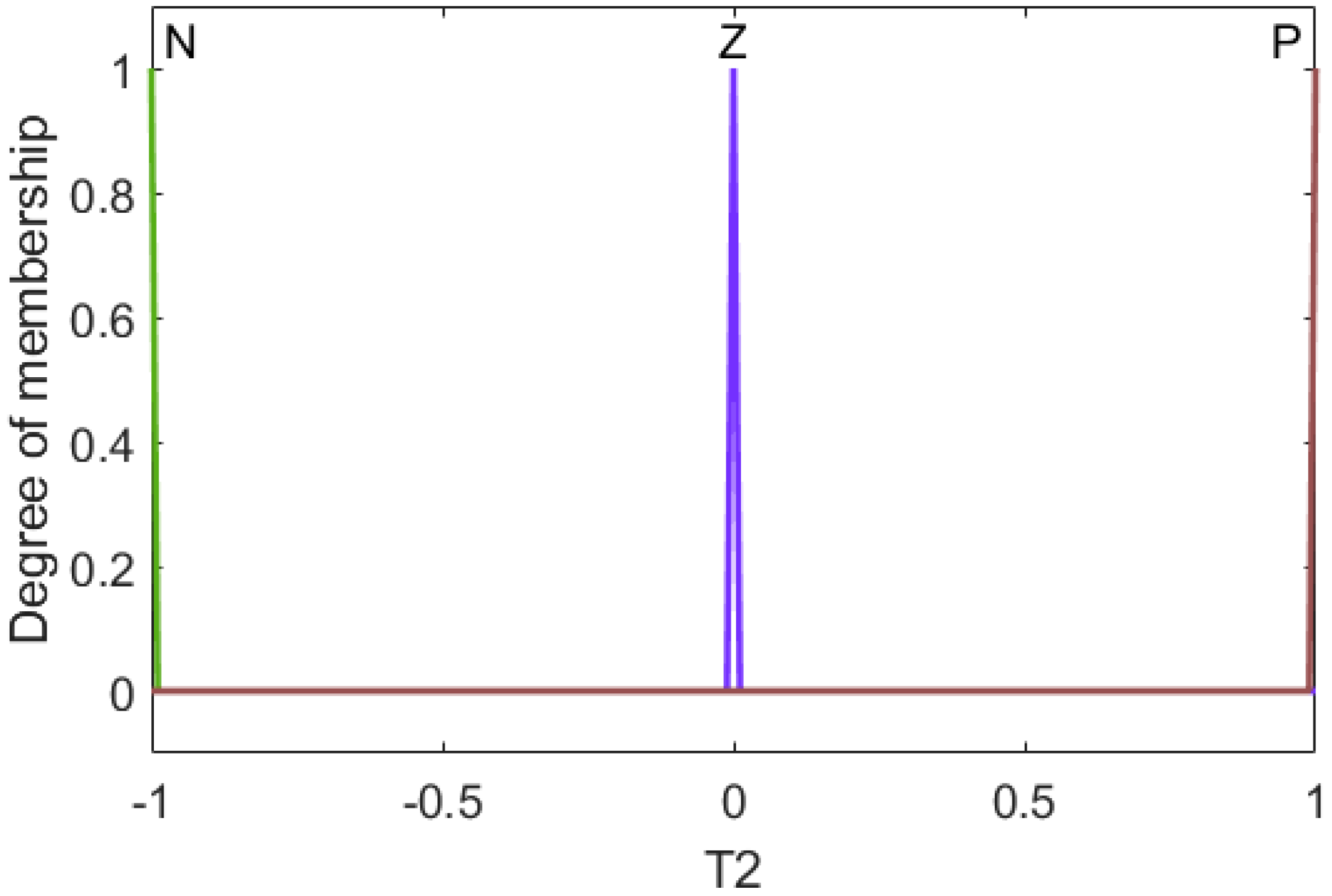
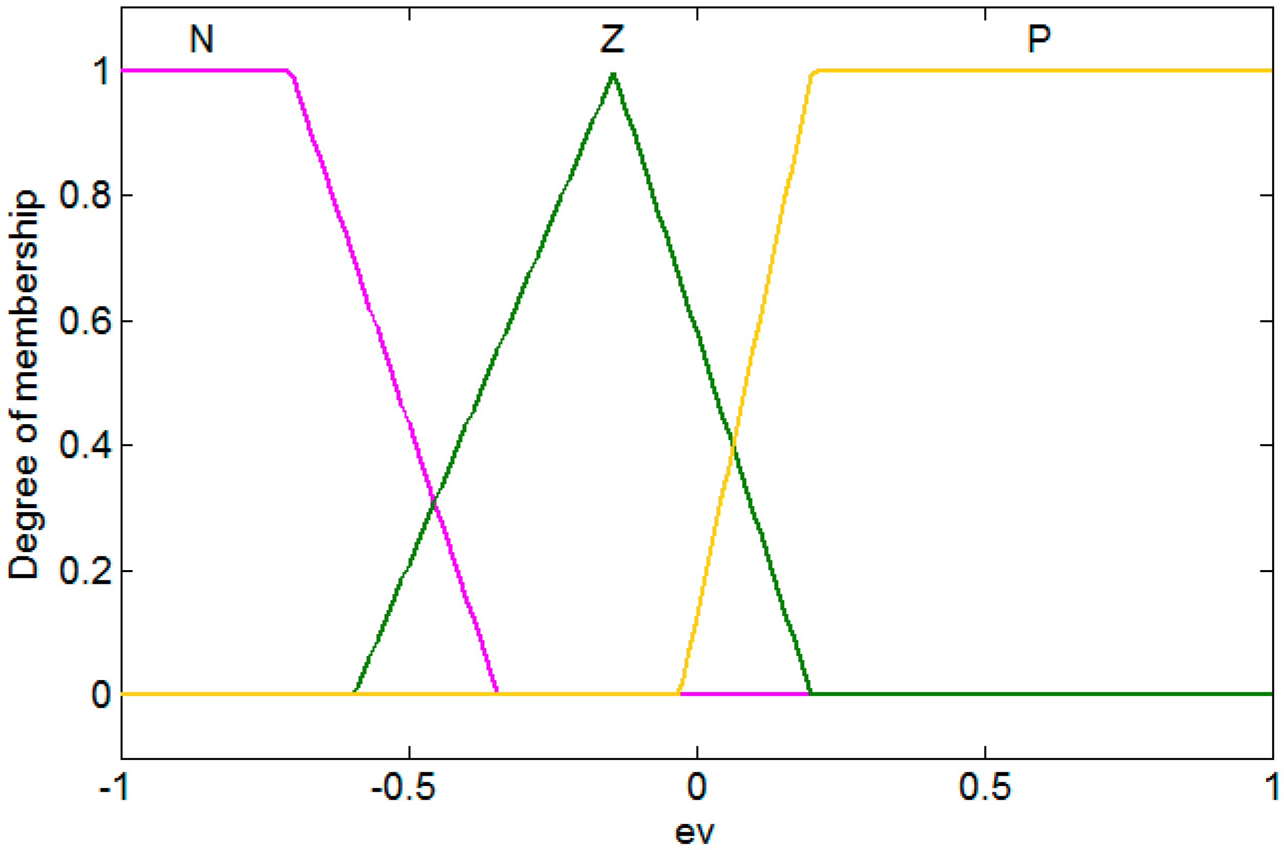
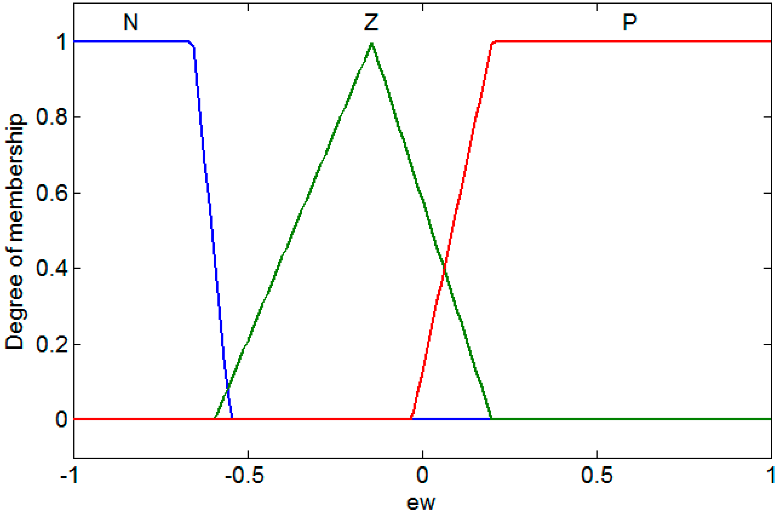
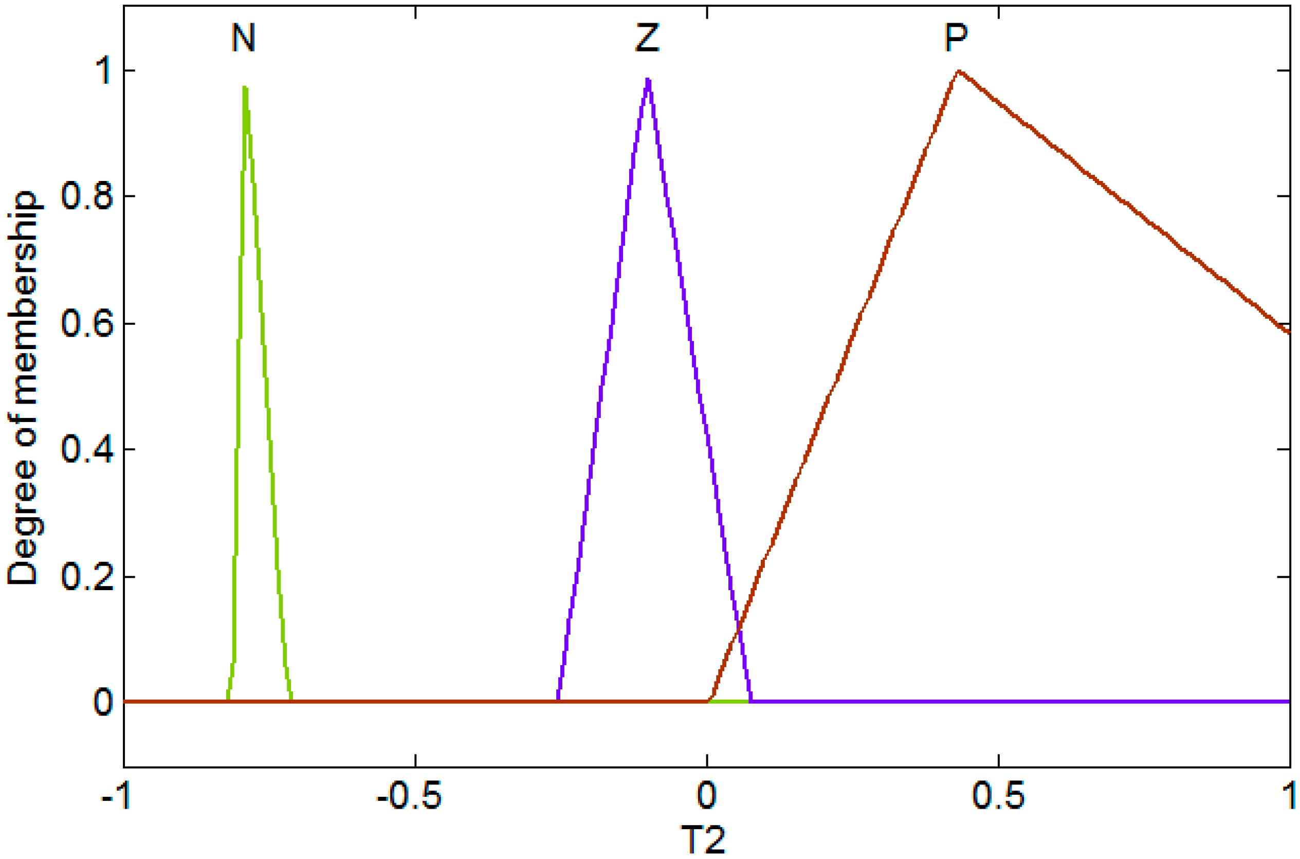
| If then Rules |
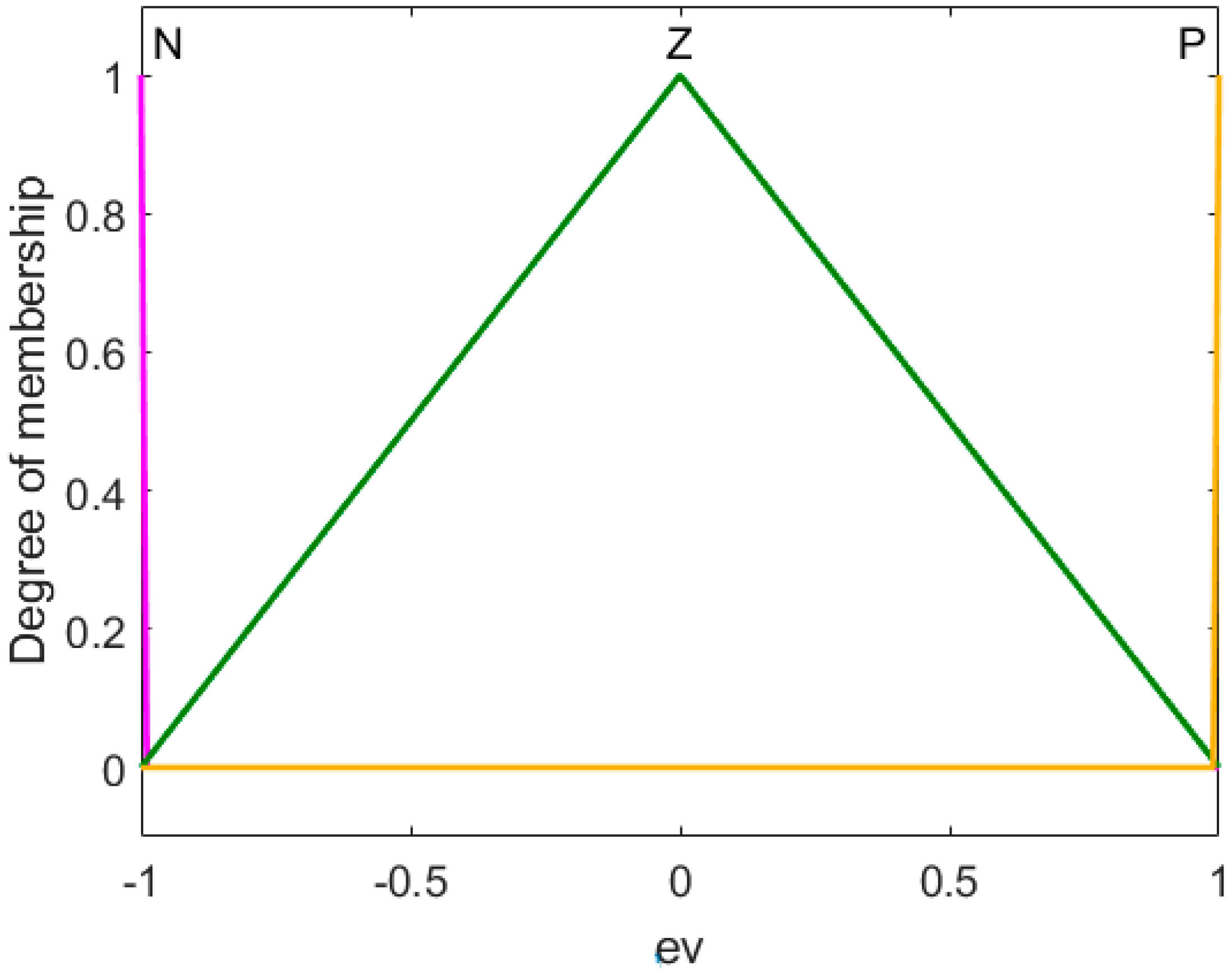
| 1. If (ev is N) and (ew is N) then (T1 is N)(T2 is N) (1) |
| 2. If (ev is N) and (ew is Z) then (T1 is N)(T2 is Z) (1) |
| 3. If (ev is N) and (ew is P) then (T1 is N)(T2 is P) (1) |
| 4. If (ev is Z) and (ew is N) then (T1 is Z)(T2 is N) (1) |
| 5. If (ev is Z) and (ew is Z) then (T1 is Z)(T2 is Z) (1) |
| 6. If (ev is Z) and (ew is P) then (T1 is Z)(T2 is P) (1) |
| 7. If (ev is P) and (ew is N) then (T1 is P)(T2 is N) (1) |
| 8. If (ev is P) and (ew is Z) then (T1 is P)(T2 is Z) (1) |
| 9. If (ev is P) and (ew is P) then (T1 is P)(T2 is P) (1) |
| Population | Iterations | Dimensions |
|---|---|---|
| 30 | 500 | 30 |
| WDO | DSO | ||||
|---|---|---|---|---|---|
| Function | fmin | Average | Standard Deviation | Average | Standard Deviation |
| f1 | 0 | ||||
| f2 | 0 | ||||
| f3 | 0 | ||||
| f4 | 0 | ||||
| f5 | 0 | 28.5696 | |||
| f6 | 0 | ||||
| f7 | 0 | ||||
| f9 | 0 | −118.27 | 0 | ||
| f10 | 0 | ||||
| f11 | 0 | 0 | 0 | ||
| f15 | 0.00030 | ||||
| f16 | −1.0316 | 1.0316 | |||
| f17 | 0.398 | 0.3979 | 0 | ||
| f18 | 3 | 7.7827 | 3 | ||
| Population | Iterations | Dimensions |
|---|---|---|
| 30 | 500 | 64 |
| WDO | DSO | ||||
|---|---|---|---|---|---|
| Function | fmin | Average | Standard Deviation | Average | Standard Deviation |
| f1 | 0 | ||||
| f2 | 0 | ||||
| f3 | 0 | ||||
| f4 | 0 | ||||
| f5 | 0 | ||||
| f6 | 0 | ||||
| f7 | 0 | ||||
| f9 | 0 | ||||
| f10 | 0 | ||||
| f11 | 0 | ||||
| f15 | 0.00030 | ||||
| f16 | −1.0316 | ||||
| f17 | 0.398 | 0 | |||
| f18 | 3 | 7.7827 | 3 | ||
| Population | Iterations | Dimensions |
|---|---|---|
| 30 | 500 | 128 |
| WDO | DSO | ||||
|---|---|---|---|---|---|
| Function | fmin | Average | Standard Deviation | Average | Standard Deviation |
| f1 | 0 | ||||
| f2 | 0 | ||||
| f3 | 0 | ||||
| f4 | 0 | ||||
| f5 | 0 | ||||
| f6 | 0 | ||||
| f7 | 0 | ||||
| f9 | 0 | ||||
| f10 | 0 | ||||
| f11 | 0 | ||||
| f15 | 0.00030 | ||||
| f16 | −1.0316 | ||||
| f17 | 0.398 | ||||
| f18 | 3 | ||||
| Figure | f1 | f1 | f1 |
|---|---|---|---|
| Iterations | 500 | 500 | 500 |
| Dimensions | 30 | 64 | 128 |
| Average | |||
| Standard Deviation |
| Function | f2 | f2 | f2 |
| Iterations | 500 | 500 | 500 |
| Dimensions | 30 | 64 | 128 |
| Average | |||
| Standard Deviation |
| Population | Iterations |
|---|---|
| 20 | 1500 |
| Experiment | MSE | Experiment | MSE |
|---|---|---|---|
| 1 | 16 | ||
| 2 | 17 | ||
| 3 | 18 | ||
| 4 | 19 | ||
| 5 | 20 | ||
| 6 | 21 | ||
| 7 | 22 | ||
| 8 | 23 | ||
| 9 | 24 | ||
| 10 | 25 | ||
| 11 | 26 | ||
| 12 | 27 | ||
| 13 | 28 | ||
| 14 | 29 | ||
| 15 | 30 |
| Experiment | MSE | Experiment | MSE |
|---|---|---|---|
| 1 | 16 | ||
| 2 | 17 | ||
| 3 | 18 | ||
| 4 | 19 | ||
| 5 | 20 | ||
| 6 | 21 | ||
| 7 | 22 | ||
| 8 | 23 | ||
| 9 | 24 | ||
| 10 | 25 | ||
| 11 | 26 | ||
| 12 | 27 | ||
| 13 | 28 | ||
| 14 | 29 | ||
| 15 | 30 |
| Experiment | MSE | Experiment | MSE |
|---|---|---|---|
| 1 | 16 | ||
| 2 | 17 | ||
| 3 | 18 | ||
| 4 | 19 | ||
| 5 | 20 | ||
| 6 | 21 | ||
| 7 | 22 | ||
| 8 | 23 | ||
| 9 | 24 | ||
| 10 | 25 | ||
| 11 | 26 | ||
| 12 | 27 | ||
| 13 | 28 | ||
| 14 | 29 | ||
| 15 | 30 |
| FA | WDO | DSO | |
|---|---|---|---|
| Average | |||
| Standard deviation |
| Variable | Number of Samples | Mean | Standard Deviation |
|---|---|---|---|
| WDO | 30 | 0.006 | 0.012 |
| DSO | 30 | 0.042 | 0.033 |
| Parameters | Value |
|---|---|
| Difference | −0.036 |
| z (Observed value) | −5.628 |
| z (Critica value) | −1.645 |
| valor-p (one-tailed) | <0.0001 |
| alpha | 0.05 |
© 2019 by the authors. Licensee MDPI, Basel, Switzerland. This article is an open access article distributed under the terms and conditions of the Creative Commons Attribution (CC BY) license (http://creativecommons.org/licenses/by/4.0/).
Share and Cite
Lagunes, M.L.; Castillo, O.; Valdez, F.; Soria, J. Multi-Metaheuristic Competitive Model for Optimization of Fuzzy Controllers. Algorithms 2019, 12, 90. https://doi.org/10.3390/a12050090
Lagunes ML, Castillo O, Valdez F, Soria J. Multi-Metaheuristic Competitive Model for Optimization of Fuzzy Controllers. Algorithms. 2019; 12(5):90. https://doi.org/10.3390/a12050090
Chicago/Turabian StyleLagunes, Marylu L., Oscar Castillo, Fevrier Valdez, and Jose Soria. 2019. "Multi-Metaheuristic Competitive Model for Optimization of Fuzzy Controllers" Algorithms 12, no. 5: 90. https://doi.org/10.3390/a12050090
APA StyleLagunes, M. L., Castillo, O., Valdez, F., & Soria, J. (2019). Multi-Metaheuristic Competitive Model for Optimization of Fuzzy Controllers. Algorithms, 12(5), 90. https://doi.org/10.3390/a12050090