A Variable Block Insertion Heuristic for Solving Permutation Flow Shop Scheduling Problem with Makespan Criterion

Abstract

In this paper, we propose a variable block insertion heuristic (VBIH) algorithm to solve the permutation flow shop scheduling problem (PFSP). The VBIH algorithm removes a block of jobs from the current solution. It applies an insertion local search to the partial solution. Then, it inserts the block into all possible positions in the partial solution sequentially. It chooses the best one amongst those solutions from block insertion moves. Finally, again an insertion local search is applied to the complete solution. If the new solution obtained is better than the current solution, it replaces the current solution with the new one. As long as it improves, it retains the same block size. Otherwise, the block size is incremented by one and a simulated annealing-based acceptance criterion is employed to accept the new solution in order to escape from local minima. This process is repeated until the block size reaches its maximum size. To verify the computational results, mixed integer programming (MIP) and constraint programming (CP) models are developed and solved using very recent small VRF benchmark suite. Optimal solutions are found for 108 out of 240 instances. Extensive computational results on the VRF large benchmark suite show that the proposed algorithm outperforms two variants of the iterated greedy algorithm. 236 out of 240 instances of large VRF benchmark suite are further improved for the first time in this paper. Ultimately, we run Taillard’s benchmark suite and compare the algorithms. In addition to the above, three instances of Taillard’s benchmark suite are also further improved for the first time in this paper since 1993.

1. Introduction

Sustainability in manufacturing industries is mainly measured by their competitiveness in the market place. Competitiveness is referred to timely product delivery with the best quality, minimum manufacturing time and price to customers. Minimum manufacturing time can be obtained by optimal production sequences that can minimize makespan or total flowtime. Note that a manufacturing company can fail to satisfy production plans although the other production entities such as operators, maintenance, inventory, quality control, etc. are in control due to the lack of optimal or near optimal production sequences in the shop floor. For this reason, seeking optimal or near-optimal production sequences and schedules is vital to manufacturing companies in order to minimize the makespan, which also minimizes idle times on the machines and maximize machine utilization.

The permutation flow shop scheduling problem (PFSP) has been widely studied in the literature and has extensively been applied in the inustry. There are many different fields in real-life where PFSP can be used [1]. It is yet an exceptionally active topic of investigation, especially because flow shop environments are at the center of real-life scheduling problems in various fields of high social or economic impact. In addition, the flow shop layout is a regular configuration in many manufacturing companies. The basic PFSP consists of a set of $n$ jobs which are processed by $m$ machines. These jobs follow the same route and their operations on the machines cannot be interrupted. All the jobs must be processed in the same order on the machines and the aim is to find the best permutation $\pi =\left\{{\pi }_1,{\pi }_2,\dots ,{\pi }_n\right\}$ of these jobs with respect to the given objective.

In this study, our aim is to maximize the throughput of the system by maximizing the utilization rate of the machines which means minimizing makespan. To compute the makespan, $\pi$ denotes the given arbitrary solution, where job ${\pi }_i$ is the job at the ith position of solution $\pi$. $C_{i,k}$ is denoted as the completion time of job ${\pi }_i$ on machine $k$ at position $i$. Following this notation, completion times of jobs at each machine are computed as in the following Equations (1)–(5), where $p_{{\pi }_i,k}$ is the processing time of job ${\pi }_i$ at the kth machine. The makespan of solution $\pi$, denoted as $C_{max}(\pi )$, is the completion time of the last job (i.e., $n$) on the last machine (i.e., $m$). It is simply denoted as $C_{nm}$ and calculated as follows:

$$C_{1,1}=p_{{\pi }_1,1}$$

(1)

$$C_{i,1}=C_{i-1,1}+p_{{\pi }_i,1}\hspace{1em}\hspace{1em}\hspace{1em}\forall i=2,\dots ,n$$

(2)

$$C_{1,k}=C_{1,k-1}+p_{{\pi }_1,k}\hspace{1em}\hspace{1em}\hspace{1em}\forall k=2,\dots ,m$$

(3)

$$C_{i,k}=max\left\{C_{i-1,k},C_{i,k-1}\right\}+p_{{\pi }_i,k}\hspace{1em}\hspace{1em}\hspace{1em}\forall i=2,\dots ,n;\forall k=2,\dots ,m$$

(4)

$$C_{max}(\pi )=C_{nm}.$$

(5)

The PFSP with makespan criterion is denoted as $Fm\left|Permu\right|Cmax$ according to the notation of [2] and has been proven to be NP-hard for the makespan criterion [3], so it is challenging to solve it with exact methods. Therefore, metaheuristic algorithms were employed to solve the problem and obtain near-optimal solutions. In recent years, various metaheuristic algorithms have been presented to solve various variants of PFSP with different objectives. One of the state-of-the-art algorithms for PFSPs is the iterated greedy algorithm (IG) presented by [4]. We focused on the recent literature that considers the IG algorithm in their solution approaches.

The IG algorithm was employed to PFSP with makespan criterion in [4,5,6,7,8,9]. In [5], to improve the solution quality, a local search was applied to the partial solution after the destruction step of the IG algorithm, while in [6] sequence depended setup times were employed for the PFSP with makespan criterion. In addition, in [7] the authors studied the PFSP with makespan and proposed a tie-breaking mechanism for the IG algorithm, while in [8] an IG and a discrete differential evolution algorithm were proposed and compared. In this study, we employ new hard VRF instances which are first introduced in [9], and they also applied an IG algorithm. In addition, the same problem was studied in [10] to minimize the makespan over Taillard’s benchmark suite.

The IG algorithm was applied to various variants of PFSP such as no-wait flow shops in [11,12,13]; blocking flow shops in [14,15,16,17]; no-idle flow shops in [18,19,20]; energy-efficient PFSP in [21,22]; multi-objective PFSP in [23,24] where both studies presented a restarted iterated Pareto greedy algorithm. In a no-wait variant of PFSP, distributed no-wait flow shop problem [11], tabu-based reconstruction strategy [12], and sequence depended setup times [13] were employed with IG algorithm. In blocking variant of PFSP, IG algorithms were combined with local search algorithms [14], constructive heuristics [15,16], and also embedded in differential evolution framework [17]. In [25] profile fitting and NEH heuristic algorithms were proposed for the same problem. In a no-idle variant of PFSP, iterated reference greedy algorithm [18], and variable IG algorithm [19] were presented. In addition, IG algorithm was employed for the mixed no-idle PFSP [20].

IG algorithm was also applied to PFSP with different objective functions such as total tardiness criterion [26,27]; total flowtime criterion [28]. In [1], they carried out an exhaustive review and computational evaluation of heuristics and metaheuristics published until 2017 for the PFSP to minimize the makespan. Therefore, for the further analysis of the literature of PFSP, the indicated manuscript [1] should be examined.

In traditional search algorithms, swap and insertion neighborhood structures are generally employed. The swap neighborhood exchanges two jobs in a solution, whereas the insertion one removes a job from a solution and inserts it into another position in the solution. Recently, block move-based local search algorithms are presented for the single machine-scheduling problems in the literature [29,30,31,32]. Xu et al. [31] developed a Block Move neighborhood structure in which $l$ consecutive jobs (called a block) are inserted into another position in the solution. They represent a block move by a $triplet(i,k,l)$, where $i$ denotes the position of the first job of the block, $k$ the target position of the block to be inserted and $l$ the size of the block. It is obvious that one edge insertion, two edge-insertion and 3-block insertion are the block move neighborhoods with $l=1$, $l=2,$ and $l=3$. Similarly, Gonzales and Vela [32] developed a variable neighborhood descent algorithm with three distinct block move neighborhoods and employed in a memetic algorithm. Then, a memetic algorithm with block insertion heuristic is presented in [29]. Moreover, in [33], a variable block insertion heuristic (VBIH) algorithm was employed to solve the blocking PFSP with makespan criterion.

In IG algorithms, some solutions components are removed from the current solution and reinserted into the partial solutions. In other words, a number, $dS$, of jobs are removed randomly, which is known as the destruction phase. Then, in the construction phase, these $dS$ jobs are reinserted into the partial solution in the same order they are removed. For each of $dS$ jobs, it makes a number $n-dS+1$ of insertions. However, the VBIH algorithm removes a block of jobs ${\pi }_b$ with size $b$ from the current solution and it makes a number $n-b+1$ of block insertions only. That is the difference between IG and VBIH algorithms.

The main contributions of the paper can be outlined as follows. VBIH is employed to solve PFSP with makespan criterion using the new hard VRF benchmark sets [9]. Detailed computational results show that VBIH algorithm outperforms two variants of the iterated greedy algorithm. 236 out of 240 instances of large VRF benchmark suite are further improved for the first time in this paper, while the results of the remaining four instances are found as the same with the current results. In addition, the formulation of two mathematical models is given to solve the small benchmark set in order to verify the results of our proposed VBIH algorithm. One hundred and eight out of 240 small instances are proven to be optimal. Therefore, this paper proposes new lower bounds with the use of an efficient algorithm, which differentiates the study from the current literature. We also show that the speed up method of Taillard is substantially effective when solving the PFSP with makespan criterion.

The remaining part of the paper is organized as follows: Section 2 introduces the formulation of PFSP including mixed integer programming (MIP) model and constraint programming (CP) model whereas Section 3 presents all the heuristic algorithms. Section 4 explains the computational results of the MIP and CP models on small VRF instances to show the solution quality of the heuristic algorithms and the limitations of the models. Section 5 reports the experimental results of the heuristic algorithms and the improvements to the large VRF instances. Finally, Section 6 summarizes the concluding remarks.

2. Mathematical Model Formulation

This paper proposes MIP and CP models to solve small VRF instances for PFSP with the makespan criterion in order to verify the solution quality of proposed heuristic algorithms. The input parameters used in the models are presented in follows:

Parameters:

$n$: Total number of jobs, $i=1,\dots ,n$

$m$: Total number of machines, $k=1,\dots ,m$

$p_{i,k}$: Processing time of job $i$ on machine $k$

$M:$ A sufficient large constant integer.

2.1. The MIP Model

The MIP decision variables, objective function and the constraints are given in the following equations. The MIP formulation of PFSP, which were proposed by Manne [34], is used.

Decision Variables:

$C_{max}$: Makespan

$C_{i,k}$: Completion time of job $i$ on machine $k$

$D_{i,j}:$ Binary variable: 1 if job $i$ is scheduled before job $j;0$, otherwise; $i<j$

MIP Model: Objective and Constraints:

$$\begin{array}{c}Min{C}_{max}\\ st:\end{array}$$

(6)

$$C_{max}\ge C_{i,m}\hspace{1em}\hspace{1em}\hspace{1em}\forall i=1,\dots ,n$$

(7)

$$C_{i,1}\ge p_{i,1}\hspace{1em}\hspace{1em}\hspace{1em}\forall i=1,\dots ,n$$

(8)

$$C_{i,k}-C_{i,k-1}\ge p_{i,k}\hspace{1em}\hspace{1em}\hspace{1em}\forall i=1,\dots ,n,\forall k=2,\dots ,m$$

(9)

$$C_{i,k}-C_{j,k}+M{D}_{i,j}\ge p_{i,k}\hspace{1em}\hspace{1em}\hspace{1em}\forall i=1\le i<j\le n,\forall k=1,\dots ,m$$

(10)

$$C_{i,k}-C_{j,k}+M{D}_{i,j}\le M-p_{j,k}\hspace{1em}\hspace{1em}\hspace{1em}\forall i=1\le i<j\le n,\forall k=1,\dots ,m$$

(11)

$$D_{i,j}\in (0,1).$$

(12)

The objective function (6) minimizes the makespan while Constraint (7) calculates the maximum completion time of all jobs on the last machine. In PFSP, all jobs follow the same route through the machines so that their final processes will be done on the last machine. Constraint (8) computes the completion time of each job on machine 1 ensuring that they cannot occur earlier than the duration of their processing time on machine 1 which is the starting machine for all jobs. Constraint (9) ensures that the completion time of each job on each machine cannot be processed before their completion time on the previous machine. Constraints (10) and (11) specify the relationship between the processing of two consecutive jobs on the same machine. Constraint (11) starts that if job $i$ precedes job $j$ in the permutation, then job $i$ should be completed before job $j$ on each machine. Otherwise, job $j$ should precede job $i$ on each machine which is shown by Constraint (10).

2.2. The CP Model

CP decision variables, objective function and the constraints are presented in the following equations using the OPL API of CP Optimizer. To express the processing times of the jobs on the machines, the model uses interval variables denoted as $JobInt$. In addition, sequence variables for the machines are defined in the model as $Machine$ which collects all these interval variables.

Decision Variables:

$JobIn{t}_{i,k}$: Interval variable for job $i$ on machine $k$ with duration $p_{i,k}$

$Machin{e}_k$: Sequence variable for machine $k$ over $\left\{JobIn{t}_{i,k}|1\le i\le n\right\}$.

CP Model: Objective and Constraints:

$$Min\left(\underset{i\in J}{\max }\left(endOf(JobIn{t}_{i,m})\right)\right)$$

(13)

$$endBeforeStart(JobIn{t}_{i,k},JobIn{t}_{i,k+1})\hspace{1em}\hspace{1em}\hspace{1em}\forall i=1,\dots ,n,\forall k=1,\dots ,m-1$$

(14)

$$noOverlap(Machin{e}_k)\hspace{1em}\hspace{1em}\hspace{1em}\hspace{1em}\hspace{1em}\hspace{1em}\hspace{1em}\hspace{1em}\hspace{1em}\forall k=1,\dots ,m$$

(15)

$$sameSequence(Machin{e}_1,Machin{e}_k)\hspace{1em}\hspace{1em}\hspace{1em}\hspace{1em}\forall k=2,\dots ,m.$$

(16)

The CP model minimizes the makespan by computing the maximum end date of each job on the last machine (13). Constraint (14) impose the precedence constraints between the consecutive operations of each job on the sequence of machines. Machines are the disjunctive resources and can process only one job at a time, which is expressed by the $noOverlap$ Constraint (15) over the sequence variables associated with machines. The relationship between sequence variables and the interval variables are provided while defining the decision variables. The last constraint $sameSequence$ (16) guarantees that all the jobs are processed in the same order on each machine. Therefore, the permutation of the jobs will be the same for each machine.

3. Meta-Heuristic Algorithms

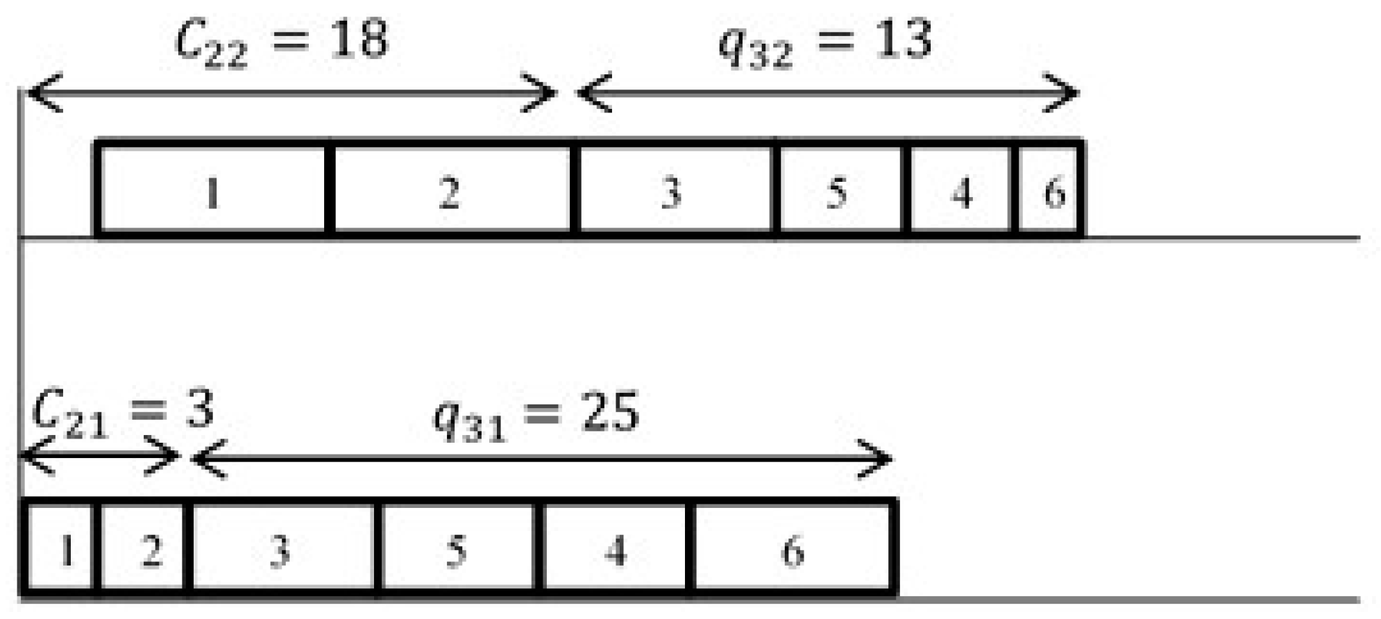
3.1. Taillard’s Speed Up Method for PFSP with Makespan Criterion

Insertion neighborhood structure is very effective for makespan minimization. The size of the insertion neighborhood is ${(n-1)}^2$. Since each objective function evaluation takes $O(nm)$ time, its computational complexity is $O(n^{3}m)$. In [35], a speed-up method is proposed where it reduces the computational complexity from $O(n^{3}m)$ to $O(n^{2}m)$ for the PFSP with makespan criterion. In order to execute the insertion procedure in time $O(nm)$, this speed-up method can be explained as follows: Suppose that job ${\pi }_i$ will be inserted in a position $l$. Then the speed up method can be described below:

• Compute the head, $e_{i,k}$, which is the earliest completion time of each job on each machine. The starting time of the first job on the first machine is 0.
  $e_{0,k}=e_{i,0}=0$             $\forall i=1,\dots ,l-1;$$\forall k=1,\dots ,m$
  $e_{i,k}=max\left\{e_{i,k-1},e_{i-1,k}\right\}+p_{{\pi }_i,k}$   $\forall i=1,\dots ,l-1;$$\forall k=1,\dots ,m$.
• Compute the tail, $q_{i,k}$, which is the duration between the starting time of each job on each machine and the end of all the operations on each machine.
  $q_{i,m+1}=0$               $\forall i=n,\dots ,l-1;\forall k=m,\dots ,1$
  $q_{l,k}$ = 0                 $\forall i=n,\dots ,l-1;\forall k=m,\dots ,1$
  $q_{i,k}=max\left\{q_{i,k+1},q_{i+1,k}\right\}+p_{{\pi }_i,,k}$   $\forall i=n,\dots ,l-1;\forall k=m,\dots ,1$.
• Compute the earliest relative completion time $f_{i,k}$ on the lth machine of job ${\pi }_j$ inserted at the lth position. Completion time of an inserted job on the first machine is zero.
  $f_{i,0}=0$                 $\forall i=1,\dots ,l$
  $f_{i,k}=max\left\{f_{i,k-1},e_{i-1,k}\right\}+p_{{\pi }_i,,k}$   $\forall i=1,\dots ,\mathrm{l}$; $\forall k=1,\dots ,m$.
• The value of the makespan $C_{max,l}$ when inserting job $j$ at the lth position is:
  $C_{max,l}=ma{x}_k(f_{ik}+q_{ik})$      $\forall i=1,\dots ,l$; $\forall k=1,\dots ,m$.

In order to illustrate the speed up the procedure, we give the 7-job 2-machine example. Note that Johnson’s algorithm [36] solves this problem to optimality. Hence, in Table 1, we provide the problem instance with the processing times as well as the optimal solution.

Table 1. Problem instance with processing times and optimal solution.

Instance			Optimal Solution with ${\mathit{C}}_{\mathit{m}\mathit{a}\mathit{x}}=36$
Jobs	M1	M2	Jobs	Position	M1	M2
1	1	8	1	1	1	8
2	2	9	2	2	2	9
3	7	5	7	3	4	5
4	5	3	3	4	7	5
5	5	4	5	5	5	4
6	7	1	4	6	5	3
7	4	5	6	7	7	1

According to the Johnson’s algorithm [36], the optimal solution is $\left\{1,2,7,3,5,4,6\right\}$ with $C_{max}=36.$ Now, suppose that we remove job 7 and obtain the partial solution, $\left\{1,2,3,5,4,6\right\}$. Suppose that we insert job 7 into position $l=3$ of the partial solution to obtain the optimal solution. We follow the speed up method now:

• Compute heads:
  $e_{0,k}=e_{i,0}=0$                     $\forall i=1,\dots ,l-1;$$\forall k=1,\dots ,m$
  $e_{i,k}=max\left\{e_{i,k-1},e_{i-1,k}\right\}+p_{{\pi }_i,k}$           $\forall i=1,\dots ,l-1;$$\forall k=1,\dots ,m$
  $e_{1,1}=max\left\{e_{1,0},e_{0,1}\right\}+p_{{\pi }_1,1}=max\left\{e_{1,0},e_{0,1}\right\}+p_{1,1}=max\left\{0,0\right\}+1=1$
  $e_{1,2}=max\left\{e_{1,1},e_{0,2}\right\}+p_{{\pi }_1,2}=max\left\{e_{1,1},e_{0,2}\right\}+p_{1,2}=max\left\{1,0\right\}+8=9$
  $e_{2,1}=max\left\{e_{2,0},e_{1,1}\right\}+p_{{\pi }_2,1}=max\left\{e_{2,0},e_{1,1}\right\}+p_{2,1}=max\left\{0,1\right\}+2=3$
  $e_{2,2}=max\left\{e_{2,1},e_{1,2}\right\}+p_{{\pi }_2,2}=max\left\{e_{2,1},e_{1,2}\right\}+p_{2,2}=max\left\{3,9\right\}+9=18$.
• Compute tails:
  $q_{i,m+1}=0$                     $\forall i=n,\dots ,l-1;\forall k=m,\dots ,1$
  $q_{l,k}$ = 0                       $\forall i=n,\dots ,l-1;\forall k=m,\dots ,1$
  $q_{i,k}=max\left\{q_{i,k+1},q_{i+1,k}\right\}+p_{{\pi }_i,k}$          $\forall i=n,\dots ,l-1;\forall k=m,\dots ,1$
  $q_{6,2}=max\left\{q_{6,3},q_{7,2}\right\}+p_{{\pi }_6,2}=max\left\{q_{6,3},q_{7,2}\right\}+p_{6,2}=max\left\{0,0\right\}+1=1$
  $q_{6,1}=max\left\{q_{6,2},q_{7,1}\right\}+p_{{\pi }_6,1}=max\left\{q_{6,2},q_{7,1}\right\}+p_{6,1}=max\left\{1,0\right\}+7=8$
  $q_{5,2}=max\left\{q_{5,3},q_{6,2}\right\}+p_{{\pi }_5,2}=max\left\{q_{5,3},q_{6,2}\right\}+p_{4,2}=max\left\{0,1\right\}+3=4$
  $q_{5,1}=max\left\{q_{5,2},q_{6,1}\right\}+p_{{\pi }_5,1}=max\left\{q_{5,2},q_{6,1}\right\}+p_{4,1}=max\left\{4,8\right\}+5=13$
  $q_{4,2}=max\left\{q_{4,3},q_{5,2}\right\}+p_{{\pi }_4,2}=max\left\{q_{4,3},q_{5,2}\right\}+p_{5,2}=max\left\{0,4\right\}+4=8$
  $q_{4,1}=max\left\{q_{4,2},q_{5,1}\right\}+p_{{\pi }_4,1}=max\left\{q_{4,2},q_{5,1}\right\}+p_{5,1}=max\left\{8,13\right\}+5=18$
  $q_{3,2}=max\left\{q_{3,3},q_{4,2}\right\}+p_{{\pi }_3,2}=max\left\{q_{3,3},q_{4,2}\right\}+p_{3,2}=max\left\{0,8\right\}+5=13$
  $q_{3,1}=max\left\{q_{3,2},q_{4,1}\right\}+p_{{\pi }_3,1}=max\left\{q_{3,2},q_{4,1}\right\}+p_{3,1}=max\left\{13,18\right\}+7=25$.

Speed-up calculation of the partial solution is given in Figure 1.

Figure 1. Speed-up calculation of a partial solution.

5.

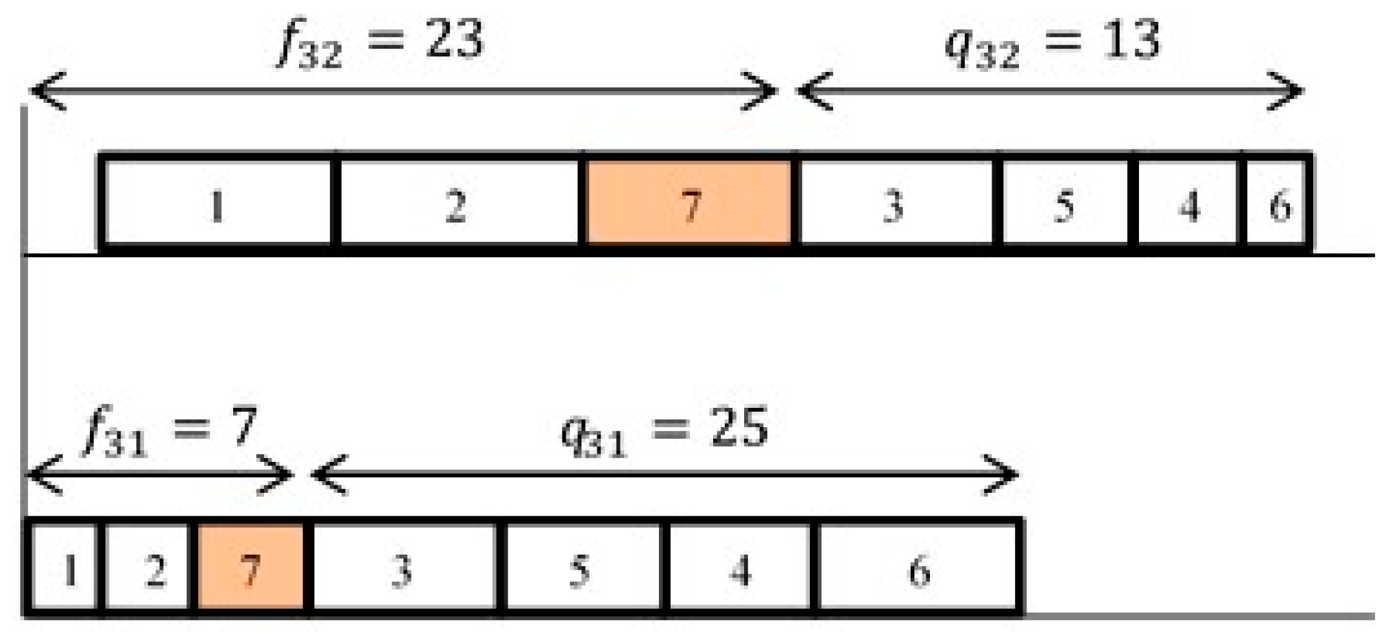
Compute the earliest relative completion time $f_{i,k}$

$f_{i,0}=0$                  $\forall i=1,\dots ,l$

$f_{i,k}=max\left\{f_{i,k-1},e_{i-1,k}\right\}+p_{{\pi }_i,k}$    $\forall i=1,\dots ,\mathrm{l}$; $\forall k=1,\dots ,m$

$f_{1,1}=max\left\{f_{1,0},e_{0,1}\right\}+p_{{\pi }_1,1}=max\left\{f_{1,0},e_{0,1}\right\}+p_{1,1}=max\left\{0,0\right\}+1=1$

$f_{1,2}=max\left\{f_{1,1},e_{0,2}\right\}+p_{{\pi }_1,2}=max\left\{f_{1,1},e_{0,2}\right\}+p_{1,2}=max\left\{1,0\right\}+8=9$

$f_{2,1}=max\left\{f_{2,0},e_{1,1}\right\}+p_{{\pi }_2,1}=max\left\{f_{2,0},e_{1,1}\right\}+p_{2,1}=max\left\{0,1\right\}+2=3$

$f_{2,2}=max\left\{f_{2,1},e_{1,2}\right\}+p_{{\pi }_2,2}=max\left\{f_{2,1},e_{1,2}\right\}+p_{2,2}=max\left\{3,9\right\}+9=18$

$f_{3,1}=max\left\{f_{3,0},e_{2,1}\right\}+p_{{\pi }_3,1}=max\left\{f_{3,0},e_{2,1}\right\}+p_{7,1}=max\left\{0,3\right\}+4=7$

$f_{3,2}=max\left\{f_{3,1},e_{2,2}\right\}+p_{{\pi }_3,2}=max\left\{f_{3,1},e_{2,2}\right\}+p_{7,2}=max\left\{7,18\right\}+5=23$.

Speed-up calculation of the complete solution is given in Figure 2.

Figure 2. Speed-up calculation of a complete solution.

6.

The value of the makespan $C_{max,l}$ when inserting job ${\pi }_i$ at the lth position is:

$C_{max,l}=ma{x}_k(f_{ik}+q_{ik})$      $i=l$; $\forall k=1,\dots ,m$

$C_{max,3}=ma{x}_k(f_{ik}+q_{ik})$

$C_{max,3}=max\left\{(f_{31}+q_{31}),(f_{32}+q_{32})\right\}$

$C_{max,3}=max\left\{(7+25),(23+13)\right\}$

$C_{max}=max\left\{32,36\right\}=36$.

It is clear that the above speed-up method reduces the complexity of the whole insertion neighborhood from $O(n^{3}m)$ to $O(n^{2}m)$. This speed-up method is the key to success for any algorithm for PFSP with makespan criterion. For this reason, we have chosen the Car8 instance from the literature in order to illustrate the speed-up method above in detail. From the literature, we know that best or optimal solution is $\left\{7,3,8,5,2,1,6,4\right\}$ with $C_{max}=8366$. In Appendix A, we remove job 2 from the optimal solution and re-insert it into the 5th position again. A detailed implementation of Taillard’s speed up method is given in Appendix A in order to ease the understanding of it.

3.2. IG Algorithms

IG algorithms mainly have four components; namely, initial solution, destruction-construction (DC) procedure, local search, and acceptance criterion. The traditional IG_RS is proposed by [4]. In this algorithm, the initial solution is constructed by the NEH heuristic in [37]. In the destruction step, $dS$ jobs are randomly removed from the solution $\pi$ without repetition and stored in ${\pi }_D$. The remaining jobs are also stored in ${\pi }_P$ that represents the partial solution. In the construction step, each job in ${\pi }_D$ is inserted into the partial solution ${\pi }_P$, in the order in which they were removed, until a complete solution of $n$ jobs is constructed. Having carried out the destruction and construction procedure, a local search is employed to further enhance solution quality. After a local search, if the solution is better than or equal to the incumbent solution, it is accepted. Otherwise, it is accepted with a simple simulated annealing-type acceptance criterion, which is suggested by [38]:

$$T=\frac{{{\displaystyle \sum }}_{j=1}^n{{\displaystyle \sum }}_{k=1}^m{p}_{kj}}{10nm}\times \tau P$$

(17)

where $\tau P$ is a parameter to be adjusted. The pseudo-code of the traditional IG_RS is given in Algorithm 1, where $r$ is a uniform random number between 0 and 1.

Algorithm 1: Traditional IGRS algorithm

$\pi =NEH$

${\pi }^{best}=\pi$

$while(NotTermination)do$

${\pi }_D=Destruction(\pi )$

${\pi }^1=\mathrm{Construction}({\pi }_D,{\pi }_P)$

${\pi }^1=LocalSearch({\pi }^1)$                      $//Algorithm 4$

$if(f({\pi }^1)\le f(\pi ))then$

$\pi ={\pi }^1$

$if(f({\pi }^1)<f({\pi }^{best}))then$

${\pi }^{best}={\pi }^1$

$endif$

$else$$if(r<exp\left\{-(f({\pi }^1)-f(\pi ))/T\right\})then$

$\pi ={\pi }^1$

$endif$

$endwhile$

$return {\pi }^{best}andf({\pi }^{best})$

The IG_RS algorithm for the PFSP under makespan minimization employs an initial solution generated by the NEH heuristic. In addition, the NEH heuristic was extended to the FRB5 heuristic with a local search on the partial solutions [39]. Both heuristics are simple and very effective for minimizing the makespan, and its pseudo-code is given in Algorithm 2. In the first phase, the sum of the processing times on all machines are calculated for each job. Then, jobs are sorted in decreasing order to obtain $\delta$. In the second phase, the first job in $\delta$ is selected to establish a partial solution ${\pi }_1$. The remaining jobs in $\delta$ are inserted in the partial solution one by one. After each iteration, optionally, a local search is applied to the partial solution. Local search is implemented as long as the partial solution is improved. After having inserted all jobs, a complete solution is obtained. Note that the NEH heuristic is denoted as FRB5 heuristic with an optional local search to partial solutions.

Algorithm 2: NEH and FRB5 constructive heuristics

$\delta =DecreasingOrder({\displaystyle \sum }_{k=1}^m{p}_{ik})$

${\pi }_1={\delta }_1$

$for i=2 to n do$

${\pi }_i=InsertJobInBestPosition({\pi }_i,{\delta }_i)$

${\pi }_i=ApplyLocalSearch({\pi }_{\mathrm{i}},f({\pi }_{\mathrm{i}}))$        $//Algorithm 3 for FRB5 heuristic$

$end for$

$return\pi with n jobs and f(\pi )$

The IG_RS algorithm employs insertion neighborhood structure as a local search after destruction and construction procedure. Insertion neighborhood is very effective with the speed-up method explained in Section 3.1 for makespan minimization. Insertion neighborhood can be deterministic or stochastic depending on the decision of choosing a job from solution to be removed. The deterministic variant is given in Algorithm 3. This procedure removes ${\pi }_i$ from the solution $\pi$ and inserts it into all possible positions of the incumbent solution $\pi$. When the best-improving insertion position is found, job ${\pi }_i$ is inserted into that position. These steps are repeated for all jobs. If an improvement is observed, the local search is re-run until no better solution is obtained.

Algorithm 3: First improvement insertion neighborhood(π)

$fori=1tondo$

${\pi }^{*}=InsertJobInBestPosition(\pi ,{\pi }_i)$

$if(f({\pi }^{*})<f(\pi ))thendo$

$\pi ={\pi }^{*}$

$endif$

$endfor$

$return \pi andf(\pi )$

In the stochastic variant given in Algorithm 4, jobs are randomly chosen from solutions to make insertions. In Algorithm 4, job ${\pi }_k$ at position $k$ is randomly chosen from the solution $\pi$ without repetition, and partial solution ${\pi }_P$ is obtained. Then, job ${\pi }_k$ is inserted into all possible positions of the partial solution ${\pi }_P$. When the best-improving insertion position is found, job ${\pi }_k$ is inserted into that position, and a complete solution ${\pi }^{*}$ is obtained. These steps are repeated for all jobs. If an improvement is found, the local search is rerun again until no better solution is obtained.

Algorithm 4: First improvement insertion neighborhood(π)

$fori=1tondo$

${\pi }_P=Remove job {\pi }_k from solution \pi randomly and without repetition$

${\pi }^{*}=InsertJobInBestPosition({\pi }_P,{\pi }_k)$

$if(f({\pi }^{*})<f(\pi ))thendo$

$\pi ={\pi }^{*}$

$endif$

$endfor$

$return \pi andf(\pi )$

Recently, a new IG_ALL algorithm has been presented in the literature [5] with excellent results for the PFSP with makespan minimization. The difference between IG_ALL and IG_RS is that IG_ALL applies an additional local search to partial solutions after destruction, which substantially enhances solution quality. In the IG_RS algorithm, local search is applied to the complete solution after the construction phase to improve the current candidate solution whereas, in IG_ALL algorithm, local search is applied to a partial solution after destruction phase. This idea is applied in heuristic algorithms by Reference [39]. They study on vehicle routing problem and apply local search on the routes in the construction phase. Applying local search to the partial solution is more advantageous in terms of computational time and providing different search directions. Due to having a partial solution, a local search is applied to the smaller size of the complete solution so that the search procedure can be conducted quickly. Another difference between IG_RS and IG_ALL is due to the fact that the initial solution is constructed by FRB5 heuristic. The pseudo code of IG_ALL algorithm is presented in Algorithm 5.

Algorithm 5: IGALL algorithm

$\pi =\mathrm{FRB}5$

${\pi }^{best}=\pi$

$While(NotTermination) do$

${\pi }_D=Destruction(\pi )$

${\pi }_P=LocalSearchToPartialSolution({\pi }_P)$          $//Algorithm 4$

${\pi }^1=Construction({\pi }_P,{\pi }_D)$

${\pi }^1=LocalSearchToCompleteSolution({\pi }^1)$         $//Algorithm 4$

$iff({\pi }^1)\le f(\pi )thendo$

$\pi ={\pi }^1$

$iff({\pi }^1)<f({\pi }^{best})thendo$

${\pi }^{best}={\pi }^1$

$endif$

$else if(r<exp\left\{-(f({\pi }^1)-f(\pi ))/T\right\})$

$\pi ={\pi }^1$

$endif$

$endif$

$endwhile$

$return{\pi }^{best}andf({\pi }^{best})$

$endprocedure$

Note that Algorithm 3 is used in the FRB5 heuristic in order to construct the initial solution with a single run due to its deterministic property. In both algorithms, Algorithm 4 is employed in applying local search to both partial and complete solutions.

3.3. Variable Block Insertion Algorithm

In this paper, we propose a VBIH algorithm as follows. The VBIH algorithm employs the FRB5 heuristic as an initial solution. It has a minimum block size $(b_{min}),$ and a maximum block size $(b_{max})$. It removes a block of jobs $({\pi }_b)$ with size $b$ from the current solution and obtains a partial solution $({\pi }_P)$. Similar to the IG_ALL algorithm, it applies the local search in Algorithm 4 to the partial solution. Then, it makes a number, $n-b+1,$ of block insertion moves sequentially in the partial solution. It chooses the best one amongst those solutions from block insertion moves. Well-known RIS local search in the literature is applied to the complete solution found after block insertion moves. If the new solution obtained after the local search is better than or equal to the current solution, it replaces the current solution. As long as it improves, it retains the same block size ($i.e.,b=b$). Otherwise, the block size is incremented by one ($i.e.,b=b+1$) and a simulated annealing-based acceptance criterion, similar to IG_RS and IG_ALL algorithms, is employed to accept the new solution to escape from local minima. This process is repeated until the block size reaches its maximum limit $(i.e.,b\le b_{max})$. The outline of the VBIH algorithm is given in Algorithm 6. Note that ${\pi }^R$ is the reference sequence; $tP$ is temperature parameter for the acceptance criterion and r is a uniform random number between 0 and 1.

Algorithm 6: VBIH algorithm

$\pi =FRB5$

${\pi }^{best}=\pi$

${\pi }^R={\pi }^{best}$

$while (NotTermination)$

$b=b_{min}=2$

$do$

${\pi }_b=Remove block {\pi }_b from \pi$

${\pi }_P=LocalSearchToPartialSolution({\pi }_P)$      $//Algorithm 4$

${\pi }^1=InsertBlockInBestPosition({\pi }_P,{\pi }_b)$

${\pi }^1=RISLocalSearchToCompleteSolution({\pi }^1)$  $//Algorithm 5$

$if (f({\pi }^1)<f(\pi )) then do$

$\pi ={\pi }^1$

$b=b$

$if (f({\pi }^1)<f({\pi }_{best}))then do$

${\pi }^{best}={\pi }^1$

${\pi }^R={\pi }^{best}$

$endif$

$else$

$b=b+1$

$if (r<exp\left\{-(f({\pi }^1)-f(\pi ))/T\right\})$

$\pi ={\pi }^1$

$endif$

$endif$

$while((b\le b_{max})$

$endwhile$

$return {\pi }^{best} and f({\pi }^{best})$

To explain the block insertion procedure, we give the following example. Suppose that we are given a current solution $\pi =\left\{1,2,3,4,5\right\}.$ Furthermore, assume that the block size is $b=2$. Let’s randomly choose a block ${\pi }_b=\left\{2,5\right\}$, thus ending up with a partial solution, ${\pi }_p=\left\{1,3,4\right\}$. After applying local search to the partial solution ${\pi }_p$, suppose that we have a partial solution ${\pi }_p=\left\{3,1,4\right\}.$ Now, the block ${\pi }_b$ is inserted into four positions as follows: ${\pi }^1=\left\{2,5,3,1,4\right\}$, ${\pi }^2=\left\{3,2,5,1,4\right\}$, ${\pi }^3=\left\{3,1,2,5,4\right\}$ and ${\pi }^4=\left\{3,1,4,2,5\right\}$. Among these four solutions, the best one will be chosen as a final solution.

Regarding the local search algorithm that will be applied only to complete solutions, we use a well-known referenced insertion scheme local search, RIS [8,40]. RIS is guided by a reference solution ${\pi }^R$, which is the best solution obtained so far during the search process. For instance, if the reference solution is given by ${\pi }^R=\left\{3,5,1,4,2\right\}$ and the current solution by $\pi =\left\{1,2,3,4,5\right\}.$ The reference solution ${\pi }^R$ implies that job 3 in the current solution $\pi$ might not be in a proper position. For this reason, the RIS local search first removes job 3 from the current solution $\pi$ and inserts it into all possible slots of the partial solution ${\pi }_P$. A new solution with the best insertion slot is replaced by the current solution, and the iteration counter is reset to one if any improvement occurs. Otherwise, the iteration counter is incremented by one. Then, it removes job 5 from the current solution $\pi$ and inserts it into all possible positions of the partial solution ${\pi }_P$. This procedure is repeated until the iteration counter is greater than the number of jobs $n$, and a new solution is obtained. The pseudo-code of the RIS local search is given in Algorithm 7.

After the local search phase, it should be decided if the new solution is accepted as the incumbent solution for the next iteration. A simple simulated annealing-type of acceptance criterion is used with a constant temperature similar to the IG_RS and IG_ALL algorithms. Note that Taillard’s speed-ups are employed wherever possible in our code.

Algorithm 7: Referenced insertion neighborhood(π)

$Count=1$

$pos=1$

${\pi }^R={\pi }^{best}$

$while (Count\le n) do$

$k=1$

$while ({\pi }_k != {\pi }_{Pos}^R) k=k+1;endwhile$    $//Find job {\pi }_k at position pos in {\pi }^R$

$pos=pos+1$

$if(pos=n+1) then$

$pos=1$

$end if$

${\pi }_P=remove {\pi }_k from \pi$

${\pi }^{*}=InsertJobInBestPosition({\pi }_P,{\pi }_k)$

$if (f({\pi }^{*})<f(\pi )) then do$

$\pi ={\pi }^{*}$

$Count=1$

$end$

$Count=Count+1$

$end if$

$endwhile$

$return \pi and f(\pi )$

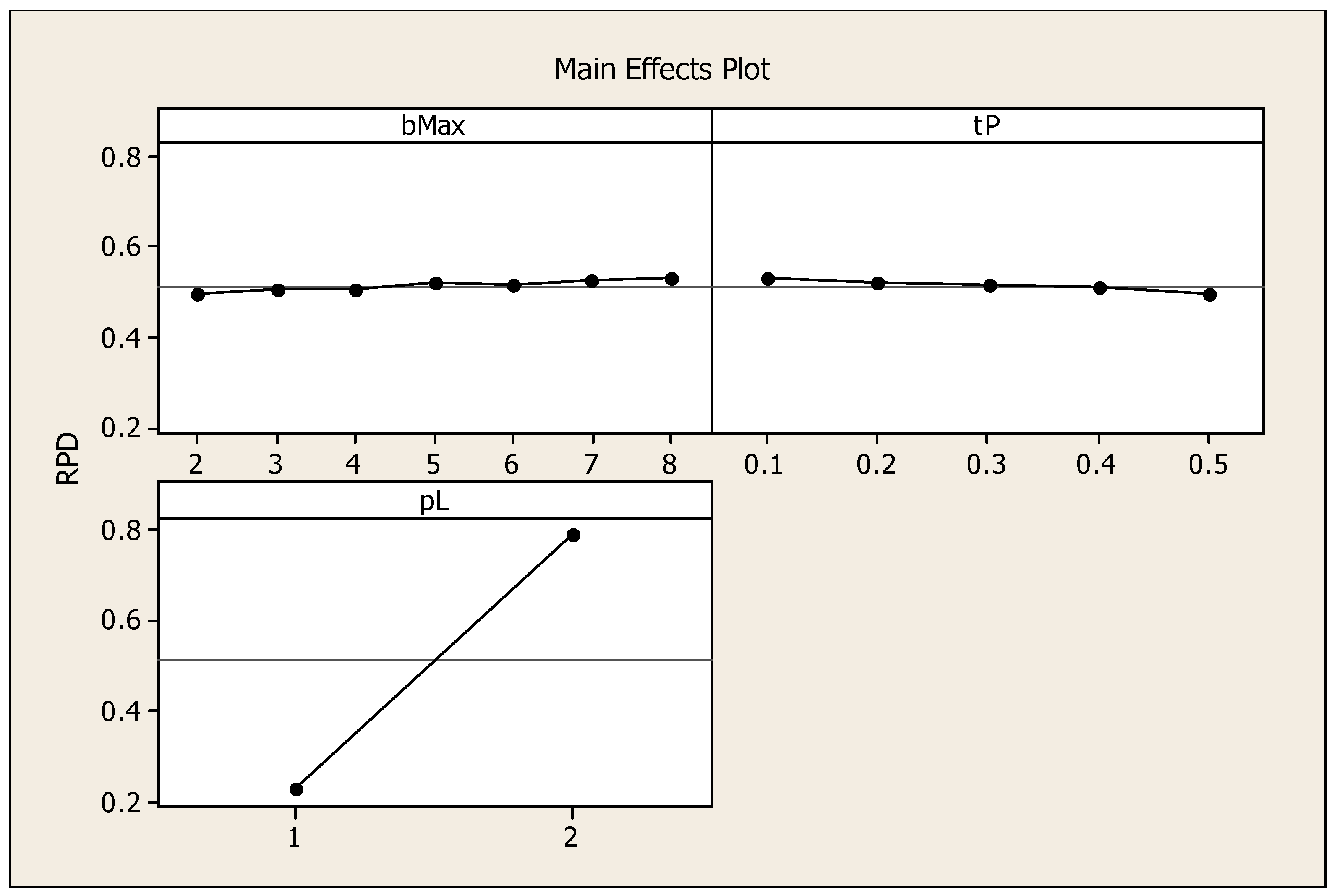
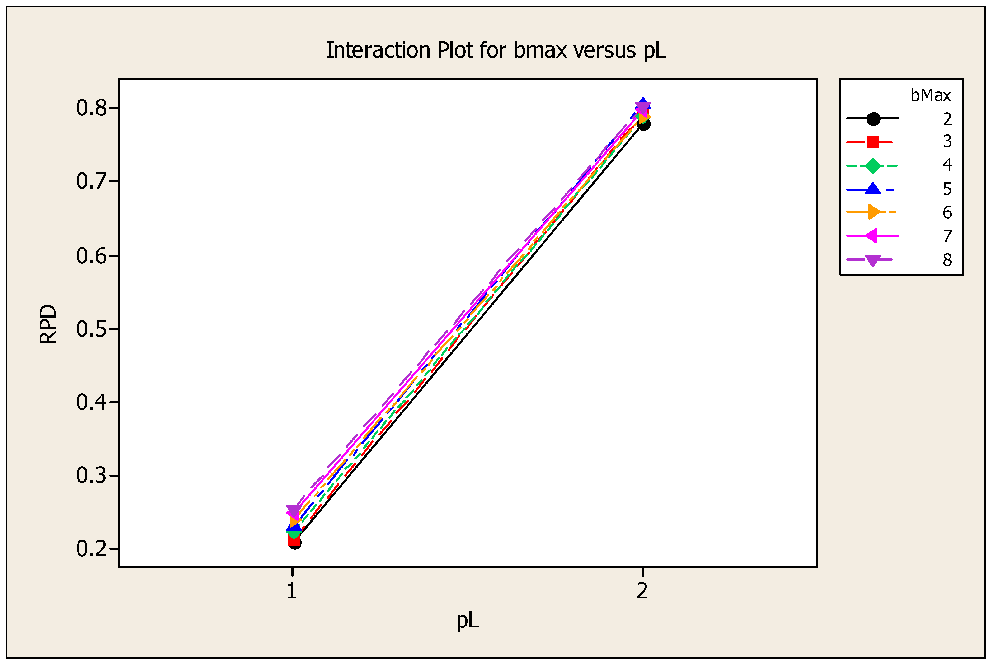
4. Design of Experiment for Parameter Tuning

In this section, we present a Design of Experiments (DOE) approach [41] for parameter settings of the VBIH algorithm. In order to carry out experiments, we generate random instances with the method proposed in [9]. In other words, random instances are generated for each combination of $n\in \left\{100,200,300,400,500,600,700,800\right\}$ and $m\in \left\{20,40,60\right\}.$ Five instances are generated for each job and machine combination. Ultimately, we obtained 1200 instances in total. We consider three parameters in the DOE approach. These are maximum block size $(bMax)$, temperature adjustment parameter ($\tau P$), and the decision of whether or not to implement the local search to the partial solution after removal of a block of jobs. We have taken the maximum block size with seven levels as $bMax\in (2,3,4,5,6,7,8)$; the temperature adjustment parameter with ten levels as $\tau P\in (0.1,0.2,0.3,0.4,0.5)$; and the decision on the local search to partial solutions as $pL\in (1,2)$. Note that $pL=1$ means that the local search is applied to partial solutions whereas $pL=2$ does not apply the local search to partial solutions. In the design of VBIH algorithm, there are $7\times 5\times 2=70$ algorithm configurations, i.e., treatments. The VBIH algorithm is coded in C++ programming language on Microsoft Visual Studio 2013, and a full factorial design of experiments is carried out for each algorithm on a Core i5, 3.40 GHz, 8 GB RAM computer. Each instance is run for 70 treatments with a maximum CPU time $T_{max}=10\times n\times m$ milliseconds. Note that it took 18 days to run the full factorial design. We calculate the relative percent deviation (RPD) for each instance-treatment pair as follows:

$$RPD=(\frac{CMA{X}_i-CMA{X}_{min}}{CMA{X}_{min}})\times 100$$

(18)

where $CMA{X}_i$ is the makespan value generated by the VBIH algorithm in each treatment and $CMA{X}_{min}$ is the minimum makespan value found amongst 70 treatments. For each job size-treatment pair, the average RPD value is calculated by taking the average of five instances in each job size. Then, the response variable (ARPD) of each treatment is obtained by averaging these RPD values of all job sizes. After determining the ARPD values for each treatment as mentioned above, the main effects plots of the parameters are analyzed and given in Figure 3.

Figure 3. Main effects plot for parameters of VBIH.

As it can be seen from Figure 3, the following parameters have better ARPD values than the others: $bMax=2$, $\tau P=0.5$, and $pL=1$. Furthermore, in order to see whether or not there is an interaction effect between parameters, an ANOVA analysis is also given in Table 2.

Table 2. ANOVA results for parameters of VBIH.

Source	DF	Seq SS	Adj SS	Adj MS	F	p-Value
$bMax$	6	0.0086	0.0086	0.0014	33.370	0.000
$tP$	4	0.0090	0.0090	0.0022	52.080	0.000
$pL$	1	5.5441	5.5441	5.5441	129,096.720	0.000
$bMax\times tP$	24	0.0010	0.0010	0.0000	0.990	0.505
$bMax\times pL$	6	0.0025	0.0025	0.0004	9.830	0.000
$tP\times pL$	4	0.0090	0.0090	0.0022	52.100	0.000
Error	24	0.0010	0.0010	0.0000
Total	69	5.5752

Table 2 indicates that $bMax$, $tP$, and $pL$ were statistically significant since higher magnitude of $F$ values and $p$-values of parameter interaction effects are less than the significance level $\alpha =0.05$. High magnitude of $F$ value for $pL$ also suggest that applying local search to partial solutions has a significant impact on the solution quality as mentioned in [5]. In terms of interaction effects, it can be observed that $bMax\times tP$ interaction is not significant because the p-value is much higher than the significance level $\alpha =0.05$. However, $bMax\times pL$ and $tP\times pL$ interactions were significant since their p values are less than the significance level $\alpha =0.05$. The interaction effects plot for $bMax\times pL$ is given in Figure 4.

Figure 4. Interaction plot for $bMax$ versus $pL$.

Figure 4 indicates that maximum block size should be taken as $bMax=2$ and local search to the partial solution should be applied. Since $tP\times pL$ interaction is also significant, we provide the interaction plot in Figure 5.

Figure 5. Interaction plot for $tP$ versus $pL$.

Figure 5 also suggests that $tP$ and $pL$ parameters should be taken as $\tau P=0.5$ and $pL=1$. Ultimately, we set the parameters of VBIH algorithm as follows: $bMax=2$, $\tau P=0.5$, and $pL=1$.

5. Computational Results

In this section, the computational results for the small and large set of VRF benchmark sets are provided. MIP and CP models were written in OPL and run on the IBM ILOG CPLEX 12.8 software suite, while all the heuristic algorithms were being written in Visual C++ 13 and carried out on an Intel Core i5, 3.40 GHz, 8 GB RAM computer. The proposed VBIH algorithm is compared to IG_RS and IG_ALL algorithms. In addition, the results of these algorithms are obtained without the Taillard’s speed up method, and they are denoted as IG_RS*, IG_ALL* and VBIH*. Regarding parameters of them with, destruction size $ds,$ and temperature adjustment factor, $tP$ are taken as $ds=4$ and $tP=0.4$ for IG_RS and IG_RS* as suggested in [4]. They are taken as $ds=2$ and $tP=0.7$ for IG_ALL and IG_ALL* as indicated in [5]. As explained in the previous section DOE is conducted for the VBIH algorithm and its parameters are determined as follows: $bMax=2$, $\tau P=0.5$, and $pL=1$, which are also used for the VBIH* algorithm.

5.1. Small VRF Instances

5.1.1. MIP Versus CP

Computational results are given in Table 3 for each combination, giving a total of 240 small VRF instances. For each combination, the table summarizes the number of optimal solutions (nOpt) found for ten instances of each job-machine combination (n × m), the average relative percent deviation (ARPD%) from the upper bounds given in [9], the average CPU time for its ten instances, and the optimality gap percentage (GAP%) on termination, which means the gap between best lower and best upper bound. The maximum CPU time is restricted to an hour (3600 s). The result of CP and MIP models are compared for job sizes 10 and 20. While MIP model can find solutions for very small sized instances (10 jobs) in a shorter time than CP model, it becomes hard for MIP to solve large sized problems (20 jobs and more). Both models cannot always find optimal solutions when the machine size becomes greater than 5, but the MIP model has larger gaps than the CP model. The results show that CP is more efficient than MIP on PFSP, except for very small-sized instances. The results of the remaining instances are obtained only from the CP model because of very large gaps by MIP model. CP model always captures optimal solutions when the machine number is five regardless of the number of jobs. Besides, CP can find optimal solutions in some of the instances when the machine size is 10. Overall, within the time limit, the CP model verifies optimality for 108 out of 240 instances.

Table 3. MIP and CP results for VRF small benchmarks with 3600 s time limit (The number in bold shows the total optimal solutions).

n × m	CP				MIP
	nOpt	ARPD	CPU	GAP	nOpt	RPD	CPU	GAP
10 × 5	10	0	14.03	0	10	0	2.68	0
10 × 10	10	0	102.13	0	10	0	4.35	0
10 × 15	10	0	256.45	0	10	0	5.68	0
10 × 20	10	0	452.79	0	10	0	9.59	0
20 × 5	10	0	2.49	0	0	0.58	3600.18	0.37
20 × 10	6	0.11	2250.09	0.03	0	2.24	3600.51	0.32
20 × 15	0	0.53	3600.05	0.13	0	2.54	3600.06	0.29
20 × 20	0	0.48	3600.07	0.17	40	2.61	3600.06	0.25
30 × 5	10	0	5.82	0	Na	Na	Na	Na
30 × 10	2	0.47	3191.89	0.05	Na	Na	Na	Na
30 × 15	0	1.29	3600.14	0.11	Na	Na	Na	Na
30 × 20	0	1.63	3600.13	0.15	Na	Na	Na	Na
40 × 5	10	0	15.03	0	Na	Na	Na	Na
40 × 10	3	0.22	3113.36	0.03	Na	Na	Na	Na
40 × 15	0	2.16	3600.10	0.10	Na	Na	Na	Na
40 × 20	0	2.11	3600.16	0.13	Na	Na	Na	Na
50 × 5	10	0	11.64	0	Na	Na	Na	Na
50 × 10	3	0.19	2939.96	0.02	Na	Na	Na	Na
50 × 15	0	2.28	3600.22	0.08	Na	Na	Na	Na
50 × 20	0	2.73	3600.22	0.12	Na	Na	Na	Na
60 × 15	10	0	6.44	0	Na	Na	Na	Na
60 × 10	4	0.19	3158.95	0.01	Na	Na	Na	Na
60 × 15	0	1.98	3600.19	0.07	Na	Na	Na	Na
60 × 20	0	2.82	3600.29	0.10	Na	Na	Na	Na
Overall Avg.	108	0.80	2146.78	0.05	40	2.61	3600.06	0.25

5.1.2. Comparison of Heuristic Algorithms with Exact Solutions

In order to compare performances of heuristic algorithms with CP exact method, we run all algorithms for five independent replications with different seed numbers. Relative percent deviation values from upper bounds for ten different instances of each job-machine combinations are calculated as follows:

$$RPD=\frac{(M-M_{UB})\times 100}{M_{UB}}$$

(19)

where $M$ is the makespan value generated by any heuristic; and $M_{UB}$ is the upper bound provided in [9]. Note that, for each instance, we record the average RFD of five replications for statistical analysis purposes, especially, for interval graphs. The solutions of the CP model are limited to 3600 s and its average CPU times are given in Table 4. IG_ALL, IG_RS, and VBIH algorithms are run for five replications with three different time limits $15$, $30$, and $45\times n\times m$. As expected, the performance of these algorithms is much better than those by CP exact model, and they improve the upper bounds provided in [9], which means that the proposed algorithm and other IG algorithms can find good (optimal in some cases) solutions in a very short time. As the solution time increases, the solution quality of VBIH algorithm increases and according to the RPD, it gives the best solutions amongst all other algorithms. It should be noted that the VBIH algorithm further improves 64 out 240 upper bounds for small VRF instances within a very short time.

Table 4. Comparison of ARPD of all algorithms for small VRF instances.

Instance	CP	15 × n × m			30 × n × m			45 × n × m
		IGRS	IGALL	VBIH	IGRS	IGALL	VBIH	IGRS	IGALL	VBIH
10 × 5	0.00	0.00	0.00	0.00	0.00	0.00	0.00	0.00	0.00	0.00
10 × 10	0.00	0.00	0.00	0.00	0.00	0.00	0.00	0.00	0.00	0.00
10 × 15	0.00	0.00	0.00	0.02	0.00	0.00	0.02	0.00	0.00	0.02
10 × 20	0.00	0.00	0.00	0.00	0.00	0.00	0.00	0.00	0.00	0.00
20 × 5	0.00	0.00	0.00	0.00	0.00	0.00	0.00	0.00	0.00	0.00
20 × 10	0.11	0.04	0.00	0.04	0.03	0.00	0.04	0.02	0.00	0.04
20 × 15	0.53	0.00	0.00	0.00	0.00	0.00	0.00	0.00	0.00	0.00
20 × 20	0.48	0.00	0.00	0.00	0.00	0.00	0.00	0.00	0.00	0.00
30 × 5	0.00	0.00	0.00	0.00	0.00	0.00	0.00	0.00	0.00	0.00
30 × 10	0.47	0.06	0.04	0.05	0.01	0.03	0.01	0.01	0.03	−0.01
30 × 15	1.29	0.03	0.02	0.03	0.02	−0.02	0.02	0.02	−0.02	0.02
30 × 20	1.63	0.02	0.00	0.03	0.02	0.00	0.02	0.02	0.00	0.02
40 × 5	0.00	0.00	0.00	0.00	0.00	0.00	0.00	0.00	0.00	0.00
40 × 10	0.22	0.06	0.02	0.03	0.02	0.01	−0.01	0.00	0.00	−0.01
40 × 15	2.16	0.09	0.05	0.04	0.04	0.02	−0.02	−0.01	−0.05	−0.05
40 × 20	2.11	0.10	−0.08	−0.04	0.04	−0.08	−0.05	−0.01	−0.08	−0.07
50 × 5	0.00	0.00	0.00	0.00	0.00	0.00	0.00	0.00	0.00	0.00
50 × 10	0.19	0.16	0.14	0.04	0.11	0.11	0.00	0.08	0.08	−0.03
50 × 15	2.28	0.24	0.18	0.10	0.15	0.14	0.05	0.10	0.09	0.02
50 × 20	2.73	0.17	0.02	0.00	0.07	−0.08	−0.10	0.04	−0.11	−0.10
60 × 5	0.00	0.00	0.00	0.00	0.00	0.00	0.00	0.00	0.00	0.00
60 × 10	0.19	0.07	0.11	−0.01	−0.04	0.08	−0.03	−0.06	0.05	−0.05
60 × 15	1.98	0.21	0.09	0.10	0.12	0.06	0.01	0.08	0.06	−0.04
60 × 20	2.81	0.20	0.01	0.00	0.03	−0.07	−0.12	−0.03	−0.08	−0.17
Avg.	0.80	0.06	0.02	0.02	0.03	0.01	−0.01	0.01	0.00	−0.02

5.2. Large VRF Instances

Note that both IG_ALL and VBIH algorithms employ the FRB5 heuristic for constructing initial solution whereas IG_RS uses the traditional NEH heuristic. For the large VRF instances, Table 5 summarizes the ARPD values of heuristic methods such as NEH, NEH without speed-up, denoted as NEH*, and extended NEH heuristic with a local search on partial solutions denoted as FRB5.

Table 5. Comparison of ARPD and computation time (CPU) for constructive heuristic methods (The number in bold shows better results).

Instance	NEH		NEH *		FRB5
	ARPD	CPU(s)	ARPD	CPU(s)	ARPD	CPU(s)
100 × 20	5.82	0.00	5.82	0.01	2.45	0.10
100 × 40	5.30	0.00	5.30	0.03	2.57	0.21
100 × 60	4.89	0.00	4.89	0.05	2.19	0.32
200 × 20	4.15	0.00	4.15	0.10	1.42	0.89
200 × 40	4.81	0.01	4.81	0.23	1.67	1.91
200 × 60	4.48	0.01	4.48	0.39	1.56	2.73
300 × 20	3.17	0.01	3.17	0.33	0.80	2.75
300 × 40	4.05	0.02	4.05	0.79	1.07	6.45
300 × 60	3.94	0.03	3.94	1.31	1.23	9.85
400 × 20	2.44	0.01	2.44	0.80	0.50	6.27
400 × 40	3.80	0.03	3.80	1.91	0.82	15.83
400 × 60	3.42	0.04	3.42	3.14	0.75	24.39
500 × 20	2.06	0.02	2.06	1.53	0.43	12.10
500 × 40	3.17	0.04	3.17	3.75	0.63	31.73
500 × 60	3.27	0.06	3.27	6.05	0.57	47.97
600 × 20	1.70	0.03	1.70	2.60	0.24	20.76
600 × 40	2.96	0.06	2.96	6.34	0.53	54.97
600 × 60	2.97	0.09	2.97	10.31	0.37	82.27
700 × 20	1.42	0.04	1.42	4.13	0.25	31.50
700 × 40	2.80	0.08	2.80	10.06	0.26	84.38
700 × 60	2.66	0.13	2.66	17.22	0.32	249.99
800 × 20	1.35	0.04	1.35	6.06	0.21	42.31
800 × 40	2.45	0.10	2.45	15.48	0.24	125.13
800 × 60	2.74	0.16	2.74	26.17	0.31	195.41
Avg	3.33	0.04	3.33	4.95	0.89	43.76

As shown in Table 5, NEH is very fast with 0.04 s on overall average CPU time. However, its overall average of ARPD is 3.33%. Although FRB5 heuristic is computationally very expensive, which is 43.76 s on overall average CPU time, its average ARPD is only 0.89% from the upper bounds. It is obvious from Table 5 that FRB5 heuristic is substantially better than NEH with a very large margin at the expense of increased CPU time. It is interesting to observe the CPU time performance of the NEH heuristic without the speed-up method of Taillard. Table 5 clearly indicates that the Taillard’s speed-up method is substantially effective since the overall average CPU time is jumped from 0.04 s to 4.95 s without the speed-up method of Taillard. In addition to the above, we present the interval graph of both constructive heuristics in Figure 6 in order for justification. Figure 6 indicates that differences in ARPDs are significantly meaningful on the behalf of FRB5 heuristic since their confidence intervals do not coincide.

Figure 6. Interval plot for small VRF instances.

5.3. Computational Results of Metaheuristics

In this section, the performance of VBIH algorithm is compared to the best-performing algorithms, IG_RS and IG_ALL, from the literature. All algorithms are run five replications to solve the large VRF instances. In Table 6, we present average, minimum and maximum ARPD values for the CPU time limit $T_{max}=15\times n\times m$ milliseconds.

Table 6. Computational results of algorithms with $T_{max}=15\times n\times m$ milliseconds (The bolds show better results).

Instance	IGRS			IGALL			VBIH
	Avg.	Min	Max	Avg.	Min	Max	Avg.	Min	Max
100 × 20	0.45	0.13	0.74	0.12	−0.07	0.33	0.00	−0.21	0.23
100 × 40	0.56	0.26	0.90	0.28	0.04	0.49	0.13	−0.09	0.37
100 × 60	0.50	0.22	0.78	0.23	0.02	0.42	0.27	0.05	0.54
200 × 20	0.42	0.24	0.61	0.19	0.04	0.35	0.03	−0.14	0.17
200 × 40	0.47	0.25	0.68	0.14	−0.01	0.31	0.01	−0.21	0.24
200 × 60	0.46	0.24	0.65	0.17	−0.01	0.37	0.05	−0.15	0.22
300 × 20	0.22	0.06	0.35	0.10	−0.03	0.21	−0.03	−0.17	0.11
300 × 40	0.35	0.15	0.56	0.04	−0.16	0.25	−0.18	−0.35	−0.02
300 × 60	0.36	0.16	0.56	0.12	−0.06	0.27	−0.03	−0.20	0.15
400 × 20	0.20	0.11	0.33	0.09	0.01	0.18	0.03	−0.03	0.10
400 × 40	0.31	0.12	0.50	0.01	−0.11	0.14	−0.17	−0.32	−0.03
400 × 60	0.27	0.08	0.46	−0.02	−0.17	0.12	−0.16	−0.27	−0.05
500 × 20	0.15	0.06	0.26	0.12	0.07	0.18	0.03	−0.05	0.12
500 × 40	0.29	0.12	0.45	0.00	−0.10	0.11	−0.19	−0.30	−0.07
500 × 60	0.33	0.15	0.51	−0.06	−0.20	0.08	−0.19	−0.31	−0.06
600 × 20	0.11	0.03	0.18	0.02	−0.03	0.07	0.01	−0.05	0.06
600 × 40	0.38	0.23	0.54	0.03	−0.07	0.13	−0.05	−0.17	0.06
600 × 60	0.30	0.12	0.50	−0.05	−0.18	0.05	−0.13	−0.23	−0.04
700 × 20	0.11	0.05	0.18	0.04	−0.01	0.08	0.03	−0.03	0.08
700 × 40	0.24	0.13	0.37	−0.11	−0.20	0.00	−0.21	−0.28	−0.12
700 × 60	0.26	0.09	0.46	−0.05	−0.15	0.04	−0.13	−0.24	−0.03
800 × 20	0.07	0.02	0.14	0.06	0.02	0.12	0.01	−0.04	0.05
800 × 40	0.22	0.09	0.36	−0.06	−0.14	0.02	−0.25	−0.33	−0.17
800 × 60	0.40	0.25	0.57	0.02	−0.04	0.08	−0.19	−0.29	−0.10
Avg	0.31	0.14	0.48	0.06	−0.06	0.18	−0.05	−0.18	0.08

As seen in Table 6, VBIH generated better Avg, Min and Max RPD values on the overall average. On overall average, it was able to further improve the upper bounds up to −0.05%; its best overall performance was −0.18% indicating that 0.18% of 240 instances are further improved and its worst-case performance was 0.08%. In order to see if differences in ARPDs are statistically significant, we provide the 95% confidence interval plot of algorithms in Figure 7, where we can observe that differences in ARPD values are statistically significant on the behalf of VBIH against IG_RS and IG_ALL algorithms because their confidence intervals do not coincide.

Figure 7. Interval plot at the 95% confidence level for large VRF instances.

Computational results for Avg, Min and Max ARPD values with the CPU time limit $T_{max}=30\times n\times m$ milliseconds are given in Table 7. As seen in Table 7, VBIH was able to generate better Avg, Min and Max ARPD values on the overall average. On overall average, it was able to further improve the upper bounds by −0.11% in Avg value, −0.24% of upper bounds are further improved on Min value and its worst-case performance was 0.02%. However, as CPU times increased, the performance of IG_ALL algorithm was also remarkable. Briefly, both VBIH and IG_ALL outperformed IG_RS in almost each problem set.

Table 7. Computational results of algorithms with $T_{max}=30\times n\times m$ milliseconds (The bolds show better results).

n × m	IGRS			IGALL			VBIH
	Avg.	Min	Max	Avg.	Min	Max	Avg.	Min	Max
100 × 20	0.25	−0.02	0.54	0.03	−0.11	0.16	−0.05	−0.25	0.16
100 × 40	0.38	0.08	0.68	0.05	−0.14	0.23	0.07	−0.15	0.33
100 × 60	0.36	0.13	0.63	0.05	−0.17	0.23	0.21	−0.02	0.51
200 × 20	0.28	0.12	0.45	0.07	−0.05	0.22	0.00	−0.16	0.14
200 × 40	0.30	0.06	0.51	−0.08	−0.25	0.08	−0.04	−0.25	0.16
200 × 60	0.26	0.05	0.51	−0.04	−0.19	0.13	0.02	−0.17	0.19
300 × 20	0.12	−0.01	0.23	0.01	−0.10	0.14	−0.06	−0.21	0.08
300 × 40	0.17	−0.03	0.41	−0.22	−0.37	−0.04	−0.23	−0.39	−0.07
300 × 60	0.18	−0.03	0.42	−0.08	−0.25	0.12	−0.09	−0.24	0.07
400 × 20	0.12	0.04	0.19	0.03	−0.04	0.09	0.01	−0.06	0.09
400 × 40	0.16	−0.03	0.37	−0.20	−0.38	−0.07	−0.22	−0.36	−0.08
400 × 60	0.08	−0.11	0.24	−0.22	−0.37	−0.07	−0.20	−0.31	−0.11
500 × 20	0.11	0.02	0.20	0.07	0.01	0.13	0.02	−0.06	0.10
500 × 40	0.13	−0.05	0.32	−0.16	−0.26	−0.06	−0.24	−0.36	−0.12
500 × 60	0.15	−0.03	0.32	−0.22	−0.35	−0.09	−0.23	−0.35	−0.10
600 × 20	0.07	−0.02	0.15	−0.01	−0.06	0.04	−0.02	−0.07	0.03
600 × 40	0.20	0.04	0.36	−0.11	−0.19	−0.02	−0.19	−0.29	−0.07
600 × 60	0.13	−0.03	0.32	−0.23	−0.37	−0.11	−0.26	−0.37	−0.15
700 × 20	0.08	0.01	0.16	0.02	−0.03	0.06	−0.01	−0.07	0.03
700 × 40	0.09	−0.01	0.19	−0.27	−0.38	−0.15	−0.34	−0.42	−0.27
700 × 60	0.07	−0.11	0.23	−0.21	−0.28	−0.13	−0.28	−0.39	−0.19
800 × 20	0.04	−0.01	0.09	0.02	−0.01	0.05	0.00	−0.04	0.04
800 × 40	0.07	−0.07	0.21	−0.20	−0.30	−0.11	−0.28	−0.35	−0.21
800 × 60	0.22	0.10	0.40	−0.13	−0.22	−0.04	−0.23	−0.32	−0.13
Avg	0.17	0.00	0.34	−0.08	−0.20	0.03	−0.11	−0.24	0.02

In order to see if these results are statistically significant, we provide the 95% confidence interval plot of algorithms in Figure 8, where we can observe that differences in ARPD values are statistically significant on the behalf of both VBIH and IG_ALL algorithms against IG_RS algorithm because their confidence intervals do not coincide with IG_RS. In other words, VBIH and IG_ALL algorithms were statistically equivalent but significantly superior to IG_RS.

Figure 8. Interval plot at the 95% confidence level for large VRF instances.

Computational results for average, minimum and maximum RPD values with the CPU time limit $T_{max}=45\times n\times m$ milliseconds are given in Table 8, where VBIH outperformed IG_RS and IG_ALL algorithms with respect to average, minimum and maximum RPD values on the overall average. On overall average, it was able to further improve the upper bounds by −0.25% on the average value, −0.36% on the minimum value, and its worst-case performance was −0.13%. These statistics indicate that VBIH generated much better results than both the IG_RS and IG_ALL algorithms.

Table 8. Computational results of algorithms with $T_{max}=45\times n\times m$ milliseconds (The bolds show better results).

n × m	IGRS			IGALL			VBIH
	Avg.	Min	Max	Avg.	Min	Max	Avg.	Min	Max
100 × 20	0.13	−0.14	0.39	−0.04	−0.21	0.1	−0.25	−0.44	−0.03
100 × 40	0.29	0.02	0.59	−0.05	−0.25	0.13	−0.18	−0.35	−0.01
100 × 60	0.26	0.03	0.48	−0.03	−0.28	0.17	−0.02	−0.17	0.19
200 × 20	0.21	0.05	0.37	0	−0.14	0.12	−0.12	−0.27	0.03
200 × 40	0.21	0.01	0.4	−0.2	−0.36	−0.03	−0.3	−0.53	−0.07
200 × 60	0.14	−0.07	0.37	−0.14	−0.3	0.02	−0.27	−0.43	−0.1
300 × 20	0.07	−0.06	0.17	−0.04	−0.18	0.1	−0.15	−0.26	−0.05
300 × 40	0.06	−0.13	0.27	−0.33	−0.47	−0.17	−0.45	−0.56	−0.28
300 × 60	0.08	−0.14	0.34	−0.24	−0.4	−0.04	−0.32	−0.47	−0.17
400 × 20	0.09	0	0.17	−0.03	−0.12	0.02	−0.05	−0.12	0.01
400 × 40	0.09	−0.09	0.3	−0.44	−0.57	−0.3	−0.41	−0.52	−0.28
400 × 60	−0.03	−0.23	0.16	−0.48	−0.64	−0.31	−0.41	−0.52	−0.32
500 × 20	0.07	−0.02	0.18	0.02	−0.06	0.08	−0.04	−0.11	0.06
500 × 40	0.04	−0.16	0.21	−0.41	−0.53	−0.29	−0.42	−0.5	−0.29
500 × 60	0.02	−0.14	0.17	−0.44	−0.56	−0.3	−0.41	−0.54	−0.29
600 × 20	0.04	−0.04	0.13	−0.04	−0.08	0.01	−0.05	−0.08	−0.01
600 × 40	0.11	−0.05	0.29	−0.32	−0.41	−0.21	−0.27	−0.39	−0.15
600 × 60	0.03	−0.12	0.22	−0.45	−0.6	−0.33	−0.35	−0.44	−0.23
700 × 20	0.06	−0.02	0.14	0	−0.05	0.05	−0.03	−0.08	0.02
700 × 40	0.01	−0.11	0.13	−0.36	−0.48	−0.24	−0.42	−0.5	−0.35
700 × 60	−0.01	−0.2	0.16	−0.3	−0.4	−0.22	−0.37	−0.48	−0.25
800 × 20	0.02	−0.04	0.07	0.01	−0.03	0.04	−0.01	−0.06	0.03
800 × 40	−0.01	−0.15	0.12	−0.27	−0.36	−0.17	−0.36	−0.43	−0.29
800 × 60	0.13	0	0.31	−0.21	−0.3	−0.14	−0.32	−0.4	−0.22
Average	0.09	−0.07	0.26	−0.20	−0.32	−0.08	−0.25	−0.36	−0.13

In order to see if these results are statistically significant, we provide the 95% confidence interval plot of algorithms in Figure 9, where we can observe that differences in ARPD values are statistically significant on the behalf of VBIH algorithm against both IG_RS and IG_ALL algorithms because their confidence intervals do not coincide. In other words, VBIH algorithm was statistically superior to both IG_RS and IG_ALL algorithm.

Figure 9. Interval plot at the 95% confidence level for large VRF instances.

In the Supplementary Materials, we summarize all the best-known solutions found for the first time by IG_ALL and VBIH algorithms. The VBIH algorithm further improves 230 out of 240 instances. In addition, 173 out of 240 instances are improved by the IG_RS algorithm, while the IG_ALL algorithm further improves 222 out of 240 instances. The IG_ALL algorithm improves six instances that are not improved by VBIH algorithm. Ultimately, 236 out of 240 instances are further improved by all algorithms within $45\times n\times m$ time limits with the remaining four solutions being equal.

As mentioned before, IG_ALL algorithm is presented in [5], where they analyzed the performances of IG_RS and IG_ALL on both Taillard’s [42] and large VRF instances. They observed that the results obtained by using Taillard’s benchmark set, both algorithms do not present very significant differences with respect to the RPDs obtained. In fact, they have shown that both algorithms did not show any statistically significant differences. However, statistically significant differences between IG_RS and IG_ALL have been shown when large VRF instances are employed. In order to validate this observation, we have run three algorithms on Taillard’s benchmark set with a stopping criterion $T_{max}=45\times n\times m$ milliseconds. Furthermore, we run three algorithms without the Taillard’s speed up method and they are denoted as IG_RS*, IG_ALL* and VBIH*. The computational results are given in Table 9. As seen in Table 9, VBIH produced much better RPDs than IG_RS and IG_ALL algorithms when the Taillard’s speed up method is employed since its overall RPD was 0.17 from the best-known solutions. However, IG_RS and IG_ALL algorithms do not show so many differences in terms of RPDs. Interval plots of the algorithms in Figure 10 show that differences in RFDs are not statistically significant because their confidence intervals do coincide. This suggests a fact that researches on PFSP and its variants should employ VRF benchmark suite to see differences in algorithms newly presented. Figure 10 also shows that the Taillard’s speed up method is significantly effective for all three algorithms. During these runs, we were also able to find 3 new best-known solutions for the Taillard’s benchmark suite (ta054 = 3719, ta55 = 3610, ta56 = 3680) and their permutations are also provided in the Supplementary Materials.

Table 9. Computational results of Taillard’s instances with $T_{max}=45\times n\times m$ milliseconds (The bolds show better results).

	IGRS	IGRS *	IGALL	IGALL *	VBIH	VBIH *
	Avg	Avg	Avg	Avg	Avg	Avg
20 × 5	0.00	0.00	0.00	0.00	0.00	0.00
20 × 10	0.01	0.00	0.00	0.00	0.00	0.01
20 × 20	0.01	0.01	0.00	0.00	0.00	0.01
50 × 5	0.00	0.00	0.00	0.00	0.00	0.00
50 × 10	0.34	0.43	0.40	0.43	0.26	0.31
50 × 20	0.57	0.79	0.53	0.71	0.33	0.53
100 × 5	0.00	0.00	0.00	0.00	0.00	0.00
100 × 10	0.10	0.19	0.04	0.11	0.02	0.09
100 × 20	0.82	1.33	0.89	1.23	0.54	0.94
200 × 10	0.05	0.14	0.03	0.05	0.03	0.05
200 × 20	1.04	1.46	0.82	1.29	0.55	1.02
500 × 20	0.47	0.92	0.35	0.75	0.26	0.64
Overall Avg.	0.28	0.44	0.26	0.38	0.17	0.30

Figure 10. Interval plot at the 95% confidence level for Taillard’s instances.

6. Conclusions

This paper presents a variable block insertion heuristic (VBIH) algorithm for solving the permutation flow shop scheduling problem (PFSP) with makespan criterion. In addition, we introduce mixed integer programming (MIP) and constraint programming (CP) models to solve the small benchmark set and to verify the results of our proposed heuristic algorithm. By employing the time limited CP model, we can find optimal solutions for some of small VRF instances for the first time in the literature. Furthermore, all algorithms can generate better solution values than upper those currently exist in the literature. We adapted a well-known speed-up method of Taillard and applied all the necessary parts while coding the heuristic algorithms. The parameters of the proposed VBIH algorithm is tuned through a design of experiments on randomly generated benchmark instances. Extensive computational results on two new VRF benchmark suites show that the VBIH algorithm is superior to the best performing algorithms from the literature.

CP model found and verify optimal solutions for 108 out of 240 small VRF instances, whereas 236 out of 240 large VRF benchmark instances are further improved by the VBIH and IG_ALL algorithms for the first time in this paper with remaining solutions being equal, which are also given in Appendix B (Table A5). Furthermore, three instances of Taillard’s benchmark suite are also further improved for the first time in this paper since 1993.

As future research, VBIH algorithm can be easily extended to other variants of the PFSPs such as no-idle, blocking and no-wait PFSP. In addition, other performance criteria can be considered such as total flow time and total tardiness. Furthermore, different meta-heuristic algorithms or matheuristics can be proposed to solve the PFSP.

References

- Fernandez-Viagas, V.; Ruiz, R.; Framinan, J.M. A new vision of approximate methods for the permutation flowshop to minimise makespan: State-of-the-art and computational evaluation. Eur. J. Oper. Res. 2017, 257, 707–721. [Google Scholar] [CrossRef]
- Pinedo, M.L. Scheduling: Theory, Algorithms, and Systems; Springer: New York, NY, USA, 2008. [Google Scholar]
- Garey, M.R.; Johnson, D.S.; Sethi, R. The Complexity of Flowshop and Jobshop Scheduling. Math. Oper. Res. 1976, 1, 117–129. [Google Scholar] [CrossRef]
- Ruiz, R.; Stützle, T. A simple and effective iterated greedy algorithm for the permutation flowshop scheduling problem. Eur. J. Oper. Res. 2007, 177, 2033–2049. [Google Scholar] [CrossRef]
- Dubois-Lacoste, J.; Pagnozzi, F.; Stützle, T. An iterated greedy algorithm with optimization of partial solutions for the makespan permutation flowshop problem. Comput. Oper. Res. 2017, 81, 160–166. [Google Scholar] [CrossRef]
- Ruiz, R.; Stützle, T. An Iterated Greedy heuristic for the sequence dependent setup times flowshop problem with makespan and weighted tardiness objectives. Eur. J. Oper. Res. 2008, 187, 1143–1159. [Google Scholar] [CrossRef]
- Fernandez-Viagas, V.; Framinan, J. On insertion tie-breaking rules in heuristics for the permutation flowshop scheduling problem. Comput. Oper. Res. 2014, 45, 60–67. [Google Scholar] [CrossRef]
- Pan, Q.-K.; Tasgetiren, M.F.; Liang, Y.-C. A discrete differential evolution algorithm for the permutation flowshop scheduling problem. Comput. Ind. Eng. 2008, 55, 795–816. [Google Scholar] [CrossRef]
- Vallada, E.; Ruiz, R.; Framinan, J.M. New hard benchmark for flowshop scheduling problems minimising makespan. Eur. J. Oper. Res. 2015, 240, 666–677. [Google Scholar] [CrossRef]
- Tasgetiren, M.F.; Pan, Q.-K.; Kizilay, D.; Velez-Gallego, M.C. A variable block insertion heuristic for permutation flowshops with makespan criterion. In Proceedings of the 2017 IEEE Congress on Evolutionary Computation (CEC), San Sebastian, Spain, 5–8 June 2017. [Google Scholar]
- Shao, W.; Pi, D.; Shao, Z. Optimization of makespan for the distributed no-wait flow shop scheduling problem with iterated greedy algorithms. Knowl. Based Syst. 2017, 137, 163–181. [Google Scholar] [CrossRef]
- Ding, J.-Y.; Song, S.; Gupta, J.; Zhang, R.; Chiong, R.; Wu, C. An improved iterated greedy algorithm with a Tabu-based reconstruction strategy for the no-wait flowshop scheduling problem. Appl. Soft Comput. 2015, 30, 604–613. [Google Scholar] [CrossRef]
- Li, X.; Yang, Z.; Ruiz, R.; Chen, T.; Sui, S. An iterated greedy heuristic for no-wait flow shops with sequence dependent setup times, learning and forgetting effects. Inf. Sci. 2018, 453, 408–425. [Google Scholar] [CrossRef]
- Ribas, I.; Companys, R.; Tort-Martorell, X. An iterated greedy algorithm for the flowshop scheduling problem with blocking. Omega 2011, 39, 293–301. [Google Scholar] [CrossRef]
- Tasgetiren, M.F.; Kizilay, D.; Pan, Q.-K.; Suganthan, P.N. Iterated greedy algorithms for the blocking flowshop scheduling problem with makespan criterion. Comput. Oper. Res. 2017, 77, 111–126. [Google Scholar] [CrossRef]
- Fernandez-Viagas, V.; Leisten, R.; Framinan, J. A computational evaluation of constructive and improvement heuristics for the blocking flow shop to minimise total flowtime. Expert Syst. Appl. 2016, 61, 290–301. [Google Scholar] [CrossRef]
- Tasgetiren, M.F.; Pan, Q.-K.; Kizilay, D.; Suer, G. A populated local search with differential evolution for blocking flowshop scheduling problem. In Proceedings of the 2015 IEEE Congress on Evolutionary Computation (CEC), Sendai, Japan, 25–28 May 2015. [Google Scholar]
- Ying, K.-C.; Lin, S.-W.; Cheng, C.-Y.; He, C.-D. Iterated reference greedy algorithm for solving distributed no-idle permutation flowshop scheduling problems. Comput. Ind. Eng. 2017, 110, 413–423. [Google Scholar] [CrossRef]
- Tasgetiren, M.F.; Pan, Q.-K.; Suganthan, P.N.; Buyukdagli, O. A variable iterated greedy algorithm with differential evolution for the no-idle permutation flowshop scheduling problem. Comput. Oper. Res. 2013, 40, 1729–1743. [Google Scholar] [CrossRef]
- Pan, Q.-K.; Ruiz, R. An effective iterated greedy algorithm for the mixed no-idle permutation flowshop scheduling problem. Omega 2014, 44, 41–50. [Google Scholar] [CrossRef]
- Ding, J.-Y.; Song, S.; Wu, C. Carbon-efficient scheduling of flow shops by multi-objective optimization. Eur. J. Oper. Res. 2016, 248, 758–771. [Google Scholar] [CrossRef]
- Öztop, H.; Tasgetiren, M.F.; Eliiyi, D.T.; Pan, Q.-K. Green Permutation Flowshop Scheduling: A Trade- off- Between Energy Consumption and Total Flow Time. In Intelligent Computing Methodologies; Springer: Cham, Switzerland, 2018; pp. 753–759. [Google Scholar]
- Minella, G.; Ruiz, R.; Ciavotta, M. Restarted Iterated Pareto Greedy algorithm for multi-objective flowshop scheduling problems. Comput. Oper. Res. 2011, 38, 1521–1533. [Google Scholar] [CrossRef]
- Ciavotta, M.; Minella, G.; Ruiz, R. Multi-objective sequence dependent setup times permutation flowshop: A new algorithm and a comprehensive study. Eur. J. Oper. Res. 2013, 227, 301–312. [Google Scholar] [CrossRef]
- Pan, Q.-K.; Wang, L. Effective heuristics for the blocking flowshop scheduling problem with makespan minimization. Omega 2012, 40, 218–229. [Google Scholar] [CrossRef]
- Karabulut, K. A hybrid iterated greedy algorithm for total tardiness minimization in permutation flowshops. Comput. Ind. Eng. 2016, 98, 300–307. [Google Scholar] [CrossRef]
- Fernandez-Viagas, V.; Valente, J.M.S.; Framinan, J. Iterated-greedy-based algorithms with beam search initialization for the permutation flowshop to minimise total tardiness. Expert Syst. Appl. 2018, 94, 58–69. [Google Scholar] [CrossRef]
- Pan, Q.-K.; Ruiz, R. Local search methods for the flowshop scheduling problem with flowtime minimization. Eur. J. Oper. Res. 2012, 222, 31–43. [Google Scholar] [CrossRef]
- Tasgetiren, M.F.; Pan, Q.; Ozturkoglu, Y.; Chen, A.H.L. A memetic algorithm with a variable block insertion heuristic for single machine total weighted tardiness problem with sequence dependent setup times. In Proceedings of the 2016 IEEE Congress on Evolutionary Computation (CEC), Vancouver, BC, Canada, 24–29 July 2016; pp. 2911–2918. [Google Scholar]
- Subramanian, A.; Battarra, M.; Potts, C.N. An Iterated Local Search heuristic for the single machine total weighted tardiness scheduling problem with sequence-dependent setup times. Int. J. Prod. Res. 2014, 52, 2729–2742. [Google Scholar] [CrossRef]
- Xu, H.; Lü, Z.; Cheng, T.C.E. Iterated Local Search for single-machine scheduling with sequence-dependent setup times to minimize total weighted tardiness. J. Sched. 2014, 17, 271–287. [Google Scholar] [CrossRef]
- Fernández, M.Á.G.; Palacios, J.; Vela, C.; Hernández-Arauzo, A. Scatter search for minimizing weighted tardiness in a single machine scheduling with setups. J. Heuristics 2017, 23, 81–110. [Google Scholar]
- Tasgetiren, M.F.; Pan, Q.-K.; Kizilay, D.; Gao, K. A Variable Block Insertion Heuristic for the Blocking Flowshop Scheduling Problem with Total Flowtime Criterion. Algorithms 2016, 9, 71. [Google Scholar] [CrossRef]
- Manne, A.S. On the Job-Shop Scheduling Problem. Oper. Res. 1960, 8, 219–223. [Google Scholar] [CrossRef]
- Taillard, E. Some efficient heuristic methods for the flow shop sequencing problem. Eur. J. Oper. Res. 1990, 47, 65–74. [Google Scholar] [CrossRef]
- Johnson, S.M. Optimal Two and Three Stage Production Schedules with Set-Up Time Included. Nav. Res. Logist. Q. 1954, 1, 61–68. [Google Scholar] [CrossRef]
- Nawaz, M.; Enscore, E.E.; Ham, I. A heuristic algorithm for the m-machine, n-job flow-shop sequencing problem. Omega 1983, 11, 91–95. [Google Scholar] [CrossRef]
- Osman, I.; Potts, C.N. Simulated Annealing for Permutation Flow-Shop Scheduling. Omega 1989, 17, 551–557. [Google Scholar] [CrossRef]
- Rad, S.F.; Ruiz, R.; Boroojerdian, N. New high performing heuristics for minimizing makespan in permutation flowshops. Omega 2009, 37, 331–345. [Google Scholar] [CrossRef]
- Tasgetiren, M.F.; Pan, Q.-K.; Suganthan, P.N.; Chua, T.J. A differential evolution algorithm for the no-idle flowshop scheduling problem with total tardiness criterion. Int. J. Prod. Res. 2011, 49, 5033–5050. [Google Scholar] [CrossRef]
- Montgomery, D.C. Design and Analysis of Experiments, 2nd ed.; Wiley: New York, NY, USA, 1984. [Google Scholar]
- Taillard, E. Benchmarks for basic scheduling problems. Eur. J. Oper. Res. 1993, 64, 278–285. [Google Scholar] [CrossRef]