1. Introduction
Experiments and computer simulations show that charged chains in free solution under an external applied electric field migrate with the same electrophoretic velocity independent of the chain size [
1] (except for very small rod-like polyions). To further derive an analytical expression for the electrophoretic velocity, the charge density within the polymer domain must be calculated and, also, the hydrodynamic friction due to the solvent [
2]. Typically, two interesting limits are considered. First, in the limit of a completely permeable coil to the solvent molecules, which flow unperturbed through the polymer coil, the fluid resistance is proportional to the degree of polymerization, or chain length
N. In the second limit, the polymer coil is viewed as an impenetrable sphere (of radius
), with a very large local segment density. The fluid resistance is that of Stokes’ law, which means that friction is proportional to chain size [
3] and scales linearly with
.
For the electrophoretic velocity
v, in the limit of small electric potentials and neglecting relaxation effects (the counterions surrounding the charged polymer are not subject to convection), Hermans and Fujita [
4,
5] obtained an analytical expression as a result of the porous sphere model, which included the dependency on the electric field
E, the radius of the porous sphere
, the internal segment density
, the hydrodynamic shielding parameter
, the fluid viscosity
η, the Debye length
, and the fixed charged density of the polyion
. It was assumed that the fluid velocity at an arbitrary position generated by applied force at the origin could be replaced in the Oseen relation by its average value over a spherical surface. We remark here that in strong confinements this cannot be strictly applicable, since there, the fluid flow velocity is highly non-isotropic. In the particular limit of completely permeable coils (
i.e.,
) the electrophoretic velocity is
, where
γ is the friction coefficient. This means that the mobility of a polyion is equal to the mobility of a segment. The other limit of a macromolecule behaving as a compact sphere (
i.e.,
) leads to the following expression,
, where
and
, in agreement with Henry’s theory [
6]. If relaxation effects are also taken into account, then, an expression for the electrophoretic velocity, which is dependent on the electric conductivities inside and, respectively, outside the polymeric domain, has been obtained by Longworth and Hermans [
7]. The inclusion of relaxation effects makes the electrophoretic velocity dependent upon the degree of polymerization, but the effect is thought to be very small.
Furthermore, Katchalsky
et al. [
8] worked out an analytical expression for the friction coefficient of the translational motion of the polymer, if the chain conformation is not Gaussian. The friction has quite a complicated dependence on the chain length, and it is not only the sum of segmental frictions, as for the case of freely-drained polymers. On the other hand, as we mentioned in the beginning, experimental results show that the mobility of the chains
, or
, if we denote by
the effective charge of the polyion, does not depend on chain length
N. Two of the most restrictive conditions were the averaging of the hydrodynamic interactions, which works well for near equilibrium transport, and the use of linearized Poisson-Boltzmann equation, if the polyions are weakly charged.
A modern review of these effects of electroosmosis and counterion penetration on electrophoresis of positively charged spherical permeable particles has been recently presented by Bhattacharyya and Gopmandal [
9]. Using numerical techniques, the authors showed good agreement with previous theories, due to Hermans and Fujita and, more recent, results by Keh and Chen [
10]. The electrical force and the hydrodynamic drag along the flow direction has been calculated by integrating on the surface of the particle the Maxwell stress tensor and hydrodynamic stress tensor. While this approach has been applied to spherical particles, its extension to arbitrary particle shapes, as for the case of confinement, is an attractive alternative to full molecular dynamics simulations.
Another recent review on DNA molecules in confinement is presented in [
11]. Experiments on electrophoresis of DNA molecules in artificial nano-channel matrices are reported by Wang
et al. [
12]. The authors find that the mobility of the strongly confined DNA depends on the degree of confinement. At strong confinement, it decreases with chain length, as is the case of gel electrophoresis, and increases at weaker confinement. Conformation dependence of DNA electrophoretic mobility in a converging channel is shown by Liao
et al. [
13]. Similar findings are presented in [
14], including the case of pulse applied electric fields or numerical investigations in [
15].
From these works, it is clear that the balance between the electrostatic forces, the hydrodynamic drag due to the solvent and the induced pressure field determine the motion of the polyions. It is our aim to investigate these effects in more detail and, in particular, for the case of confinement. Here, the macroscopically observed linear relationship between friction force and contact area can be extended to the nanoscale, with the contact area being proportional to the number of interacting atoms across the contact. There are, however, interesting effects related to surface friction, as we shall see below, if surface roughness forbids the stretching of the chains. Related experimental work showing a reduction of fluid friction atop undulating surfaces is presented, for example, by Vlachogiannis and Hanratty [
16] and more recent mesoscopic simulations of pressure-driven fluid flow in periodically grooved microchannels by Kasiteropoulou [
17].
Figure 1.
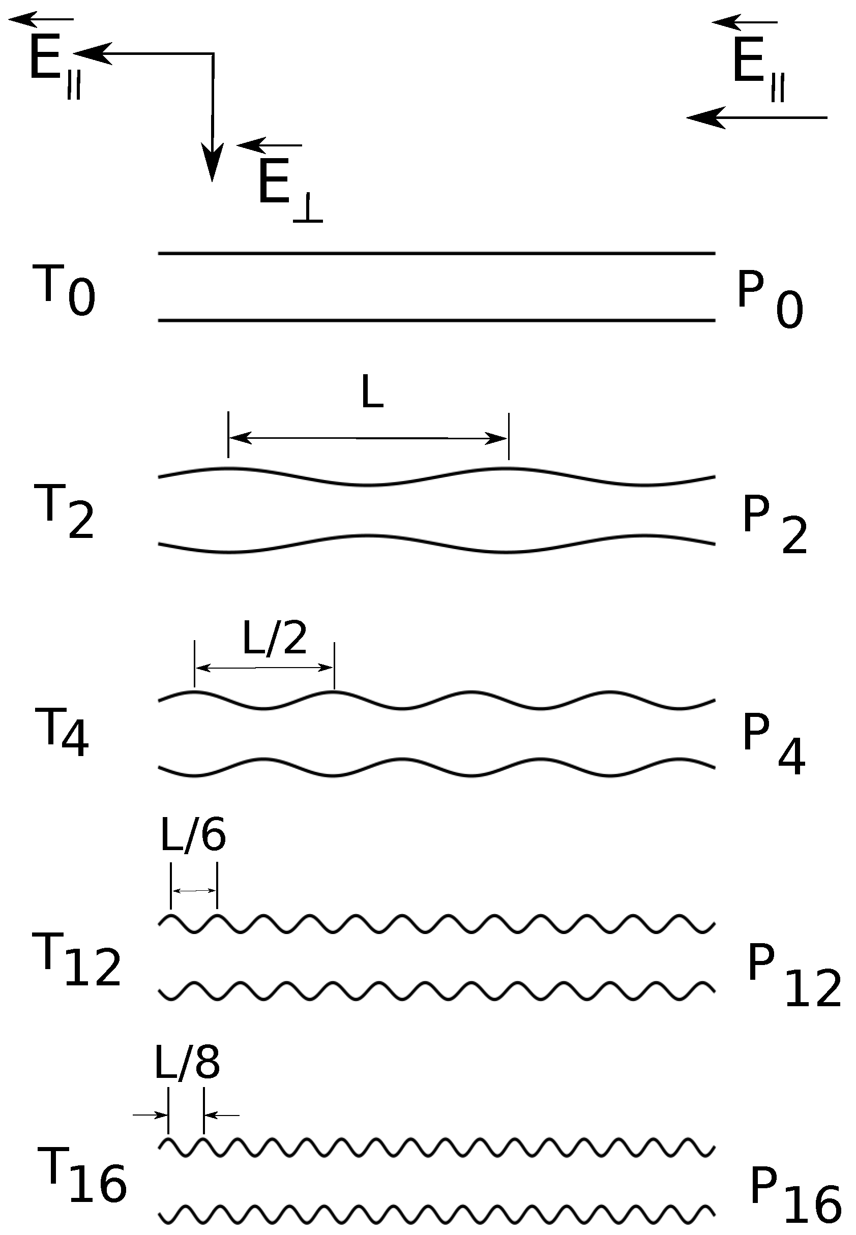
Cross-section schematic illustration (from top to bottom) of constant radius () and variable diameter straight cylinders of increasing surface undulations. The depth of surface undulations is constant, of the cylinder radius. denotes the combination of straight cylinders and parallel applied electric fields , denotes the combination of straight cylinders and both parallel and transverse applied fields , etc.
Figure 1.
Cross-section schematic illustration (from top to bottom) of constant radius () and variable diameter straight cylinders of increasing surface undulations. The depth of surface undulations is constant, of the cylinder radius. denotes the combination of straight cylinders and parallel applied electric fields , denotes the combination of straight cylinders and both parallel and transverse applied fields , etc.
In the present simulations, the shape of the confinement is either a straight cylinder or a cylinder with periodically varying diameter. The applied field can have: a longitudinal component
, in the axial direction only or both a longitudinal and a transverse component
. In
Figure 1, we present a schematic representation of the geometries. We briefly answer here the question of why do we need such a setup? First of all, the component
is the driving field, which has the same role as a pressure gradient [
18]. Second, the transverse component
enforces a separation of electroosmotic flows of counter ions and ions of added salt. We showed earlier that such separation improves resolution [
19]. In the present study, we go a step further and estimate quantitatively electrolyte friction coefficients and fluid flow velocities inside the charged polymers. The surface undulations are introduced in order to understand the interrelation between geometry shape and electrolyte friction.
2. Method
The charged polymers are bead-spring models consisting of
N beads, each carrying a unit negative electric charge and connected by a finitely extensible nonlinear elastic (FENE) potential,
, with spring constant
, and maximum extension,
, where
σ is the unit length and
is the unit energy. To simulate salt conditions, we added monovalent counterions with a concentration of
and also coions, such that the system is electrically neutral. All charged monomers interact with each other through Coulomb interactions,
, where we set
, which is the Bjerrum length of the solution. The distance between charged groups on the polyelectrolytes is
, which means that the charge density is
and condensation of counterions does not occur [
20]. All the particles (polymer or fluid monomers, counterions, coions) are modeled as spheres that interact by purely repulsive Lennard-Jones (LJ) potential,
, which is cut at
and shifted to zero. Here, we choose
. The walls of the confinement are made of uncharged monomers, which are assigned fixed positions in space. The length of the simulation box is much larger than the contour length of the charged chain. For example, we choose a minimum cylinder length of
and a maximum of approximately
for the longest chain. In all cases, the number density of counterions (and coions) was changed accordingly to the set value of
. Similarly, for any length of the simulation box, the number density of fluid monomers was fixed at
. Periodic boundary conditions are imposed in one direction only, along the cylinder axis. The fluid monomers are explicitly modeled as spherical particles and interact with all the other particles through the Lennard-Jones potential. We choose the same radius for all particles. The number density of fluid monomers is set to
. We use a Nosé-Hoover thermostat. In all studied cases, the applied longitudinal electric field is
and the transversal field is
, in units of
. We note here that for the chosen concentration of free charges, the Debye length is
. This characteristic length scale of the system becomes less defined for the case of transverse fields where there is a separation of flows of counterions and coions of salt and the system is not homogenous. The time step used in the simulations is
in units of
, and the mass of each particle is unity. All physical quantities are, therefore, given in reduced Lennard-Jones units.
The radius of the uniform straight cylinder is
, and the depth of surface undulations is
of the cylinder radius; the minimum cylinder radius is
and the maximum is
(
Figure 1). The surface undulations are sinusoidal waves of fundamental frequency
, where
. Geometries
and
have frequency
;
and
have frequency
;
and
have frequency
;
and
have frequency
.
The hydrodynamic friction force, , experienced by a charged polymer monomer is proportional to the difference between the velocity of the bead, , and the velocity of the fluid, , at the location of the bead, . The beads of the polyion are hydrodynamically interacting with each other, and the flow at the position of, say, bead i include perturbations due to the other beads, counterions and coions of added salt. In our simulations, the solvent is explicit, and therefore, the fluid velocity is obtained by averaging the instantaneous velocities of solvent monomers around each bead, i. The friction forces are, thus, position- and configuration-dependent.
In
Figure 2, we show how the local fluid velocity around an arbitrary monomer of the charged chain is computed. The calculation proceeds as follows: we index all monomers of the charged chain from one to
N. We set, then, a distance
r, which is the radius of a spherical domain
, around each monomer,
. After this, we make a list of all fluid monomers contained in all volumes
, which were drawn around each monomer,
, within distance
r, from the polyelectrolyte. In this list, some fluid monomers may appear twice, because the spherical volumes
overlap. We identify, then, all unique fluid monomers contained in all volumes
, of distance
r from the polyelectrolyte. Since the velocities of all fluid monomers are known, we compute the time averages for distances between
r and
, where
is a small parameter of the order of
σ. The final result for a chain with
monomers, for some geometries, is shown in
Figure 3. The fluid velocities are in the reference frame of the laboratory and projected on the z-axis (the direction of the longitudinal field). As expected, at large distances from the polyion the relative velocities are close to zero, while the largest values are in the immediate vicinity of the charged polymer, where the fluid is mostly perturbed. The averages are taken every 1000 time steps, while the total number of time steps for each chain length and each geometry is about
steps.
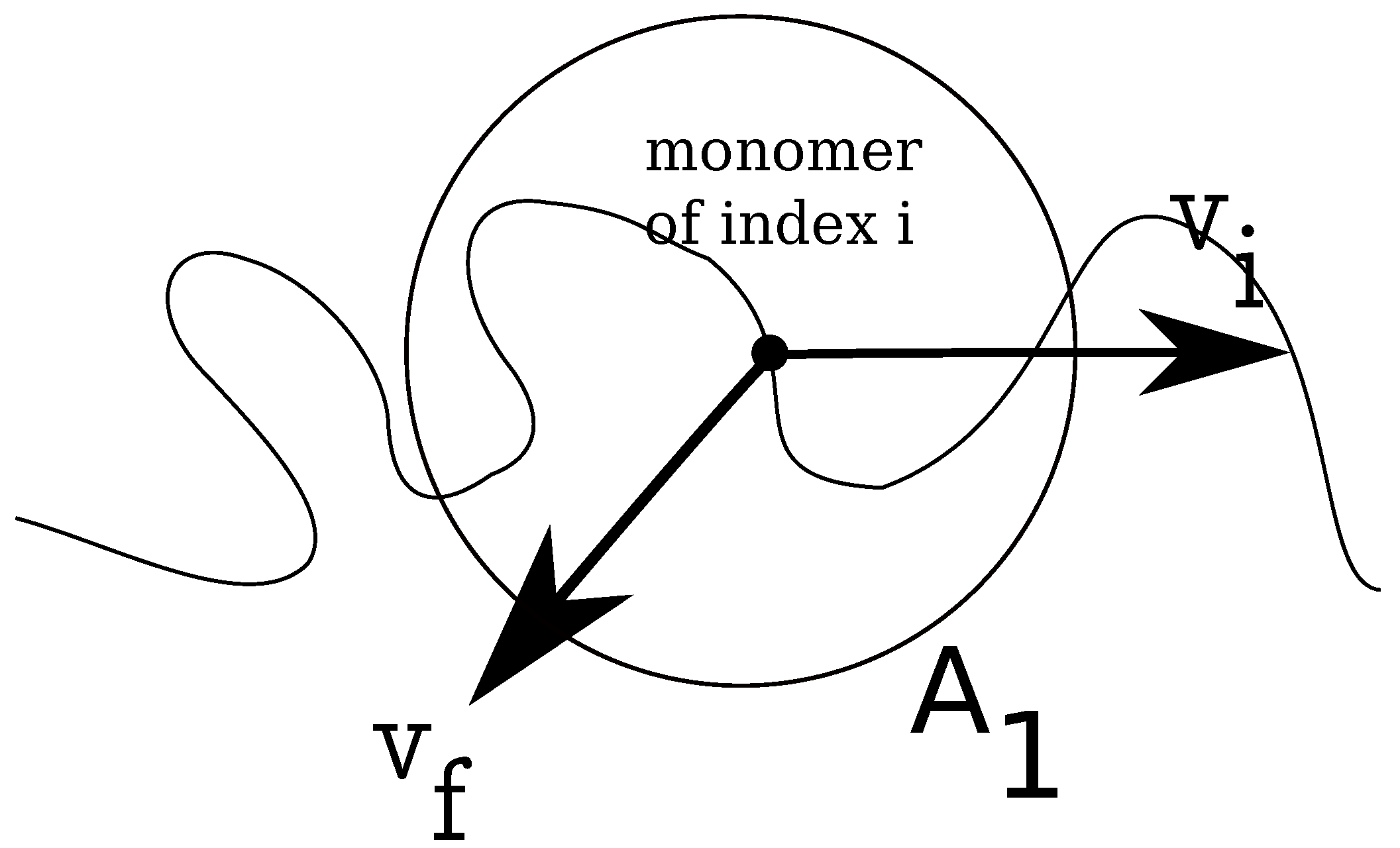
Figure 2.
Schematic illustration of fluid control volume, , around an arbitrary monomer of a charged chain, which has instantaneous velocity . The local fluid velocity at the position of monomer i is noted .
Figure 2.
Schematic illustration of fluid control volume, , around an arbitrary monomer of a charged chain, which has instantaneous velocity . The local fluid velocity at the position of monomer i is noted .
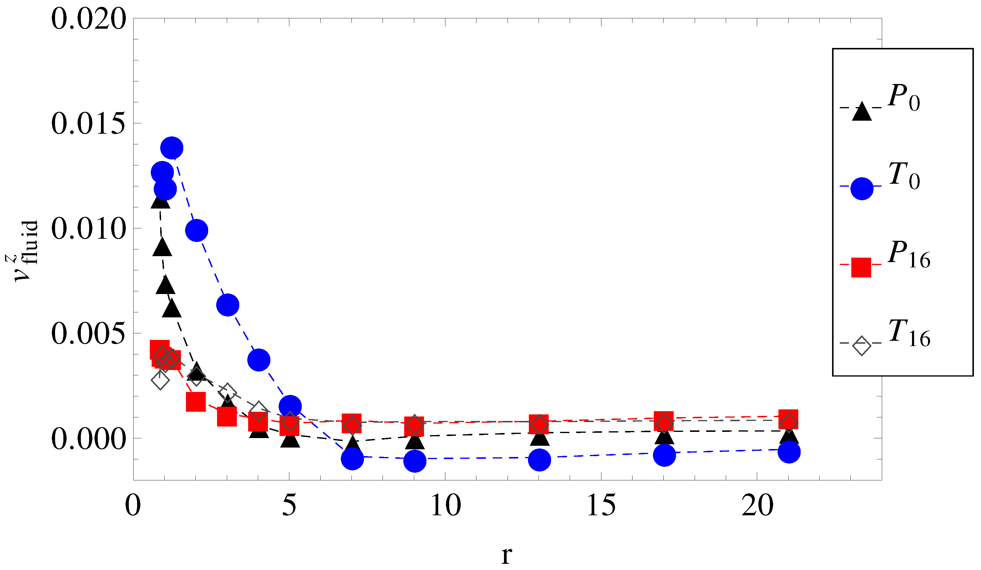
Figure 3.
The axial component of the fluid velocity around the polyion as a function of radial distance
r, for
. The legend notation is the same as in
Figure 1.
Figure 3.
The axial component of the fluid velocity around the polyion as a function of radial distance
r, for
. The legend notation is the same as in
Figure 1.
By plotting, for example, the average fluid velocity,
, and the number of counterions contained in a spherical shell of radius
r, as a function of distance
r from the center of the macroion, Chatterji and Horbach [
21] were able to estimate the role of effective charges in the electrophoresis of highly charged colloids.
With respect to the role played by electrolyte friction effects, which are retardation effects due to the counterions flowing in the opposite direction to the polyelectrolyte and slow coions flowing alongside the charged polymer, we estimate these retardation forces, of electric nature, from Schurr’s expression for the static friction of a colloidal macroion [
22]. Assuming that the fixed point charge on a bead of the polymer is
, each of these charges interact with each other and with the free ions through Coulomb forces,
, where
are point charges representing monovalent counterions and salt ions. The distance between
and
is noted with
;
and
ϵ are the permittivity of the free space and, respectively, the relative permittivity of the solvent. In Schurr’s theory, it is assumed that the fluctuating force on the polyion due to the small ions is completely uncorrelated with that due to the solvent, and therefore, the fluctuating ionic force contributes an independent additive contribution on top of the Stokes friction. The electrolyte friction is obtained from the time integral of the auto-correlation function of Coulomb forces:
Such theoretical developments are quite powerful and show an excellent good agreement with experiments. Moreover, Schurr’s theory is parameter-free. The detailed calculation of electrolyte friction in Equation (
1) is as follows: at an arbitrary time,
t, for each charged polymer monomer,
, we choose an arbitrary distance,
r, and draw a control volume,
, around each monomer of the charged chain, similar to the problem of estimating the local fluid velocity (
Figure 2). Further, we calculate the relative distances between the free ions contained in the respective volume
, and the monomer
i, which allows us to estimate the Coulomb forces
on each monomer
, where
is the coordinate of monomer
i. We define monomeric friction coefficients from the time integral of the auto-correlation function of Coulomb forces as follows:
where
is the average Coulomb force exerted on the polyelectrolyte at time,
t, by the free ions. The total electrolyte friction is the average of individual coefficients:
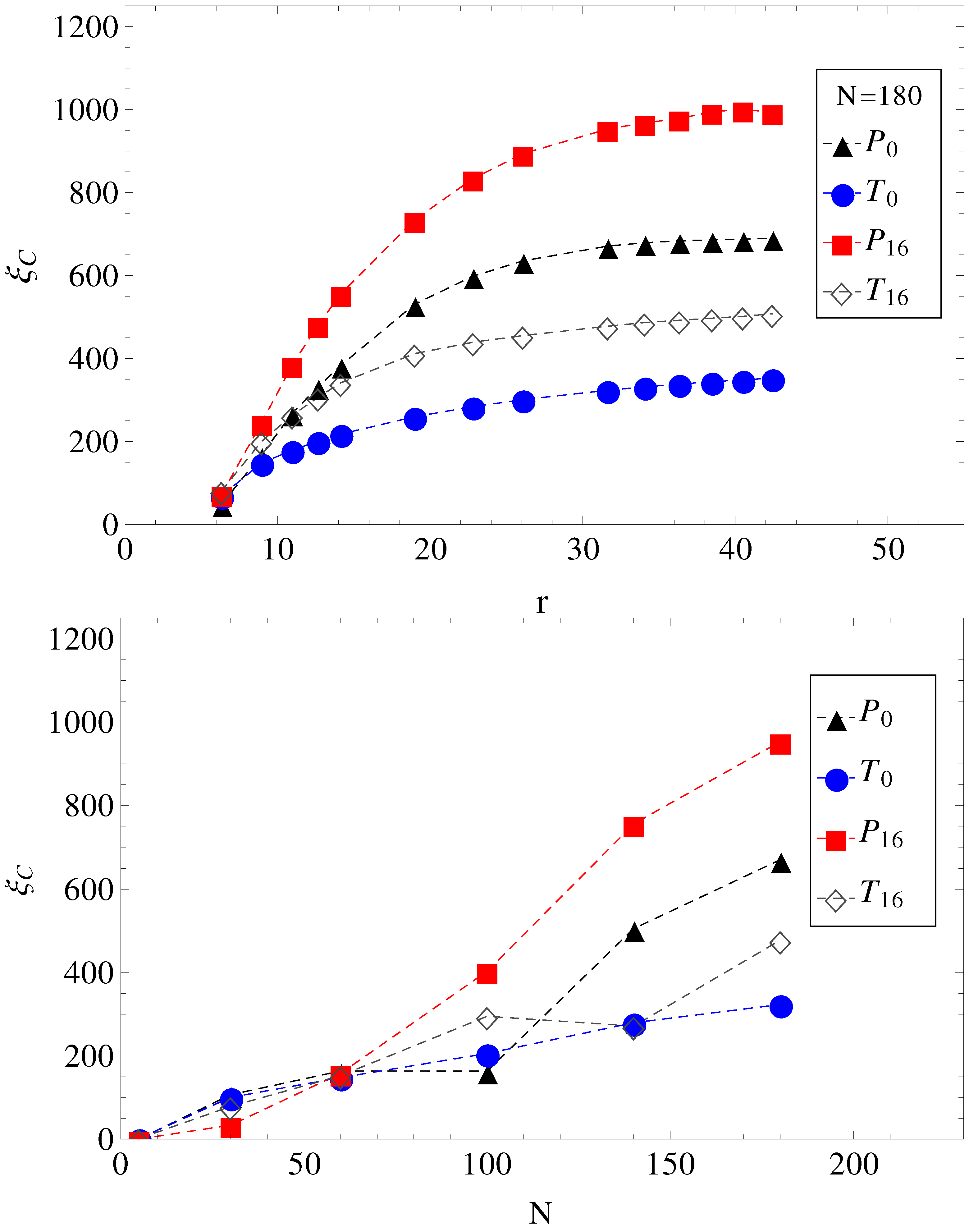
In
Figure 4, we show the electrolyte friction as a function of distance
r, for
, and the plateau values
, at large
r for the other chain lengths. We apply the same formalism, also, when a transverse electric field is superimposed on the driving longitudinal electric field. We remark here that the term under the integral in Equation (
2) has a fast exponential decay in time, but also presents a long time tail that decays as
, which is an indication of hydrodynamic memory effects [
23].
3. Results and Discussion
Here, we consider equal longitudinal and transverse electric fields,
i.e.,
in LJ units and fixed ionic strength of the buffer solution. Only the length
N of the charged chains and the number of undulations per wavelength are varied (
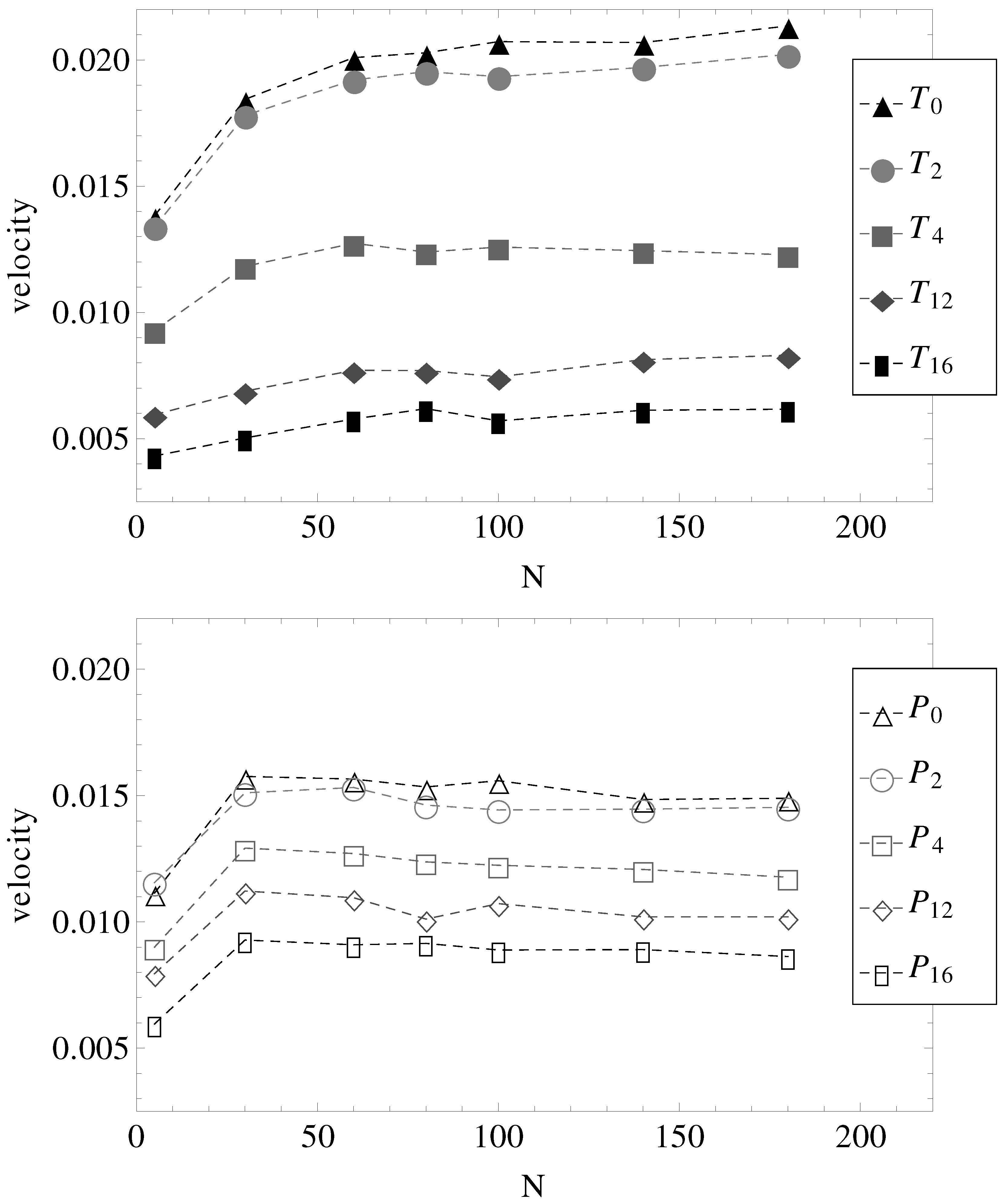
Figure 1). The measured electrophoretic velocities of the charged chains are presented in
Figure 5. Two observations are most important.
First, in parallel fields (geometries –), all chains with have more or less the same electrophoretic velocity. It appears, therefore, that by introducing surface undulations, the electrophoretic velocities decrease in value, but remain independent of N. It can be straightforwardly assumed that in these cases, the hydrodynamic, electrolyte and surface friction forces all scale with the same power of N.
The second observation concerns the effect of the transverse electric field. It appears that in nearly smooth cylinders with both longitudinal and transverse electric fields (geometries
and
), there is a slight increase in electrophoretic velocities, at least up to chain lengths
. Perhaps more remarkable, in geometries
and
, the electrophoretic velocities are higher than in geometries
and
, while in geometries
and
, the velocities are lower than in geometries
and
(
Figure 5).
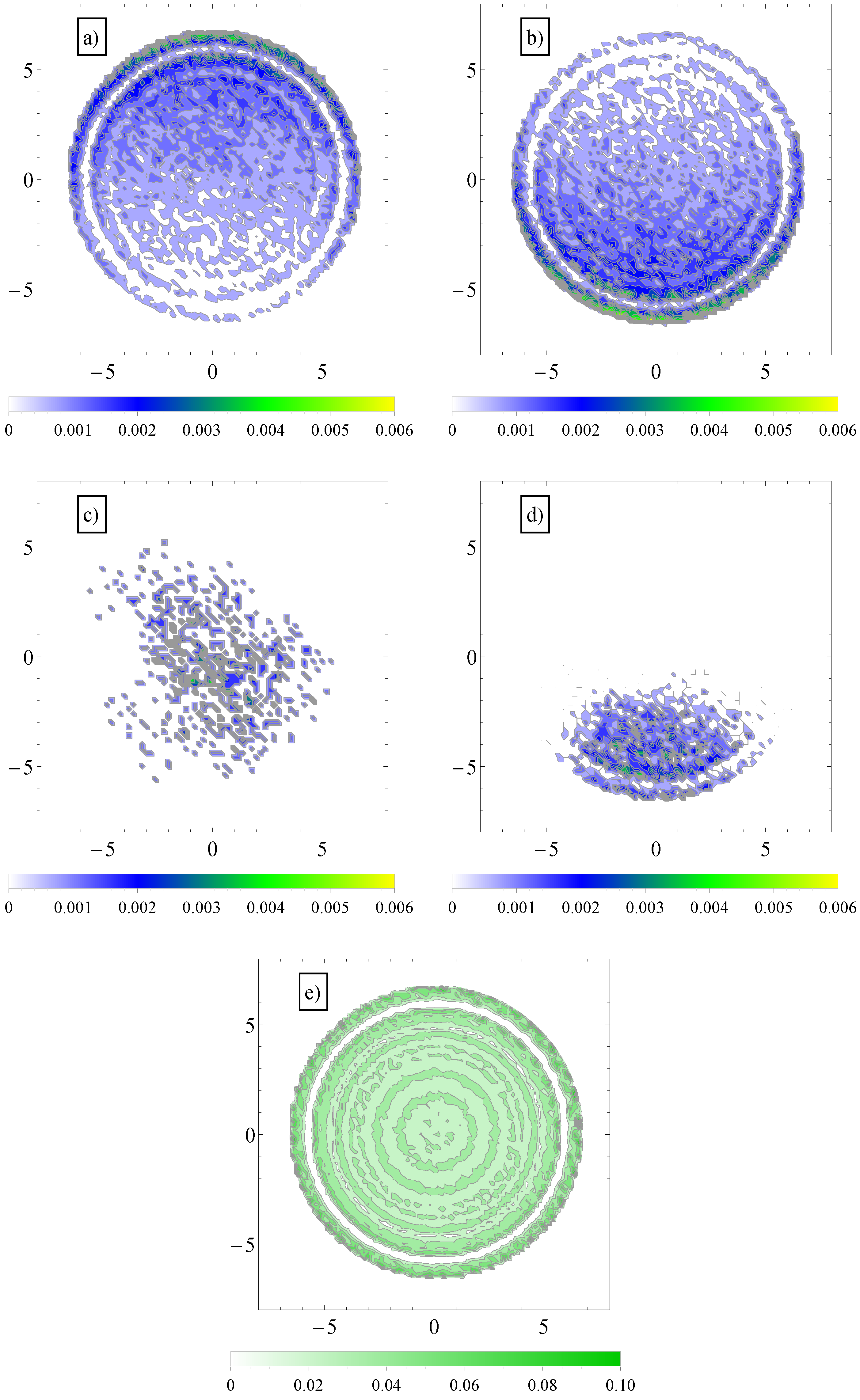
To explain this effect, we note first that in transverse fields, there is a separation of electro-osmotic flows of counterions and coions of salt. We show these two distributions in
Figure 6.
Figure 4.
(Top) Electrolyte friction as a function of distance r from the polyelectrolyte () for limiting cases of smooth and, respectively, wavy surfaces, in parallel (geometries , ) and in parallel with perpendicular applied fields (geometries , ). (Bottom) Plateau values (large r) of electrolyte friction as a function of chain length N for the same geometries, , , and .
This separation effectively creates two fluid streams, each flowing in opposite direction to each other. The polyelectrolytes swim in the fluid stream created by the coions of added salt. Because it is mostly surrounded by coions, which flow in the same direction, there are less counterions heading in the polyelectrolyte way, and therefore, there is less retardation from counterions. The conclusion is that a transverse field always makes polyelectrolytes move faster. This can be seen, for example, in
Figure 4. The electrolyte friction in
is smaller than in
. Similarly, the electrolyte friction in
is smaller than in
. This means that electrolyte friction effects alone predict the inequalities,
and
. However, this is not true. Only
is true, and
is false.
Figure 5.
Electrophoretic velocities of charged chains of length
N in uniform (index “0”) and variable diameter straight cylinders (indices “2”, “4”, “12” and “16” are in the increasing order of the number of undulations per wavelength, as shown in
Figure 1). (Top) The constant applied electric field has both longitudinal and transverse components. (Bottom) The constant applied electric field is parallel to the symmetry axis.
Figure 6.
(a) Contour plot of average number density distribution of counterions and (b) coions of added salt in a cross-section perpendicular to the axis of the cylinder geometry, . The applied field has both a longitudinal, , and a transversal component, ; (c) Similar contour plots of average number density distribution of polymer chain monomers (in the largest section area) in longitudinal fields and (d) in both longitudinal and transversal applied fields; (e) Similar distribution of fluid monomers in geometry, . In the vicinity of the walls, the monomers arrange themselves in layers.
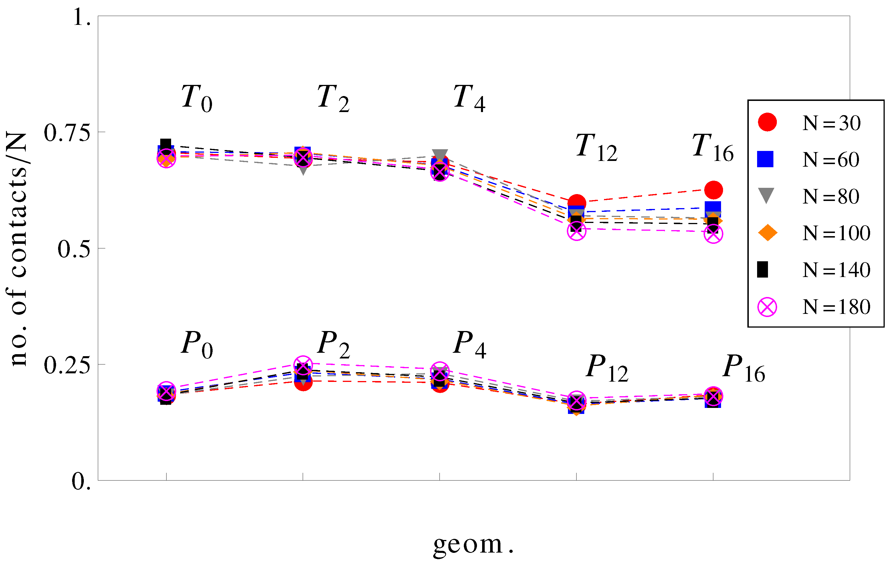
It can be further assumed that in geometries with a high number of surface undulations, the surface friction plays a predominant role in retarding the motion of the charged chains. In this respect, we calculated the average number of contacts between polyions monomers and the walls of the confinement (
Figure 7). As expected, the number of contacts is higher in cases where the perpendicular field pushes the charged chains onto the walls of the confinement than in cases where there is no transverse field. This means that surface friction effects alone would give the inequalities,
and
. While this is true, surface friction cannot explain why
. It may also appear unexpected that the number of contacts with the walls decreases when the number of undulations increases (compare, for example, geometries
and
in
Figure 7). In these situations (
,
), the chains shrink compared to geometries
and
and cannot stretch in the direction of motion. The number of contacts is therefore reduced. The average relative extensions
of the chains in the
z-direction, where
and
are the
z-coordinates of the leftmost and rightmost monomers, are shown in
Figure 8.
Figure 7.
Average number of contacts with the walls, normalized by chain length
N as a function of geometry (see
Figure 1). The top curve is for applied fields with both longitudinal and transversal components, and the bottom curve is for fields parallel to the symmetry axis.
Figure 7.
Average number of contacts with the walls, normalized by chain length
N as a function of geometry (see
Figure 1). The top curve is for applied fields with both longitudinal and transversal components, and the bottom curve is for fields parallel to the symmetry axis.
Considered separately, electrolyte friction and surface friction forces cannot predict the full correct order of velocities,
. Hydrodynamic friction alone cannot predict it either. The fluid velocity around the polyion (
) as a function of the radial distance
r in smooth and wavy geometries was shown in
Figure 3. It is readily understood that in geometry
, the fluid is partially trapped inside the polymeric domain (at
,
approaches
), which means that from a hydrodynamic point of view, the transverse field makes the charged chains less porous to the fluid flow. This means that their hydrodynamic friction is reduced, because the hydrodynamic friction is proportional to the difference between the polyelectrolyte velocity and the local fluid velocity. In other words, the transversal field perturbs the free-draining property of the chains by moving the counterions away from the polymeric domain. We assume that this effect can explain the apparent increase in velocities in
Figure 5 for geometries
and
. On the other hand, as the number of undulations increases, the hydrodynamic resistance also increases, either in longitudinal or in transverse fields. It follows that electrolyte, hydrodynamic and surface friction effects are necessarily linked together and responsible for the observed velocities of the polyelectrolytes in confinement. If we restrict ourselves to smooth cylinder geometries, we can use the above understanding of the effect of transversal fields in order to improve separation resolution. For example, the applied field can be set to
for an arbitrary time interval and then switched to
for the same time interval. The scenario corresponds to pulsed longitudinal and transversal fields. The average velocities are shown in
Figure 9 and are, in a first order approximation, equal to the mean of velocities,
and
, taken from
Figure 5, geometries
and
. It is clear that above
, separation can be achieved up to the longest chain length. Such calculations are a work in progress and will be detailed in a future publication.
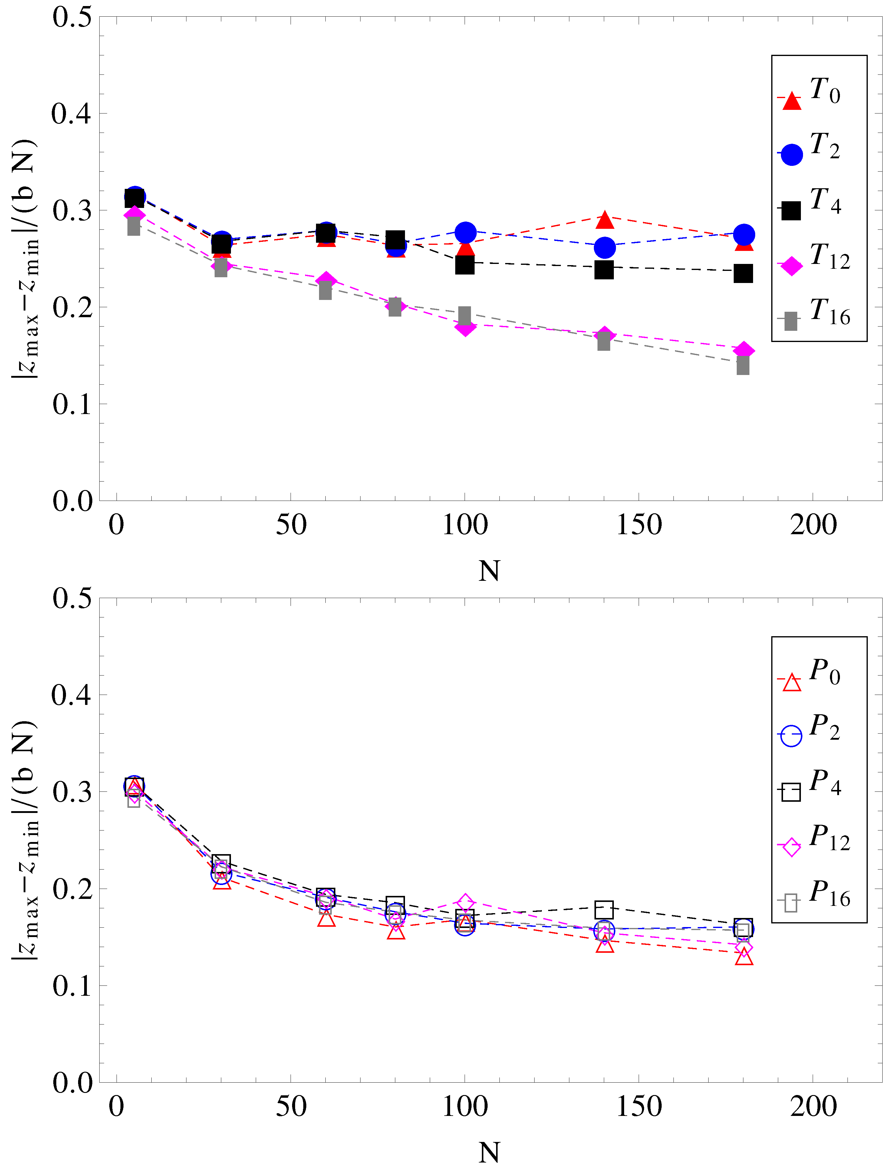
Figure 8.
Projections of charged chain extension on the z-axis, normalized by average bond length
b, and chain length
N, as a function of chain size (for legend, see
Figure 1).
Figure 8.
Projections of charged chain extension on the z-axis, normalized by average bond length
b, and chain length
N, as a function of chain size (for legend, see
Figure 1).
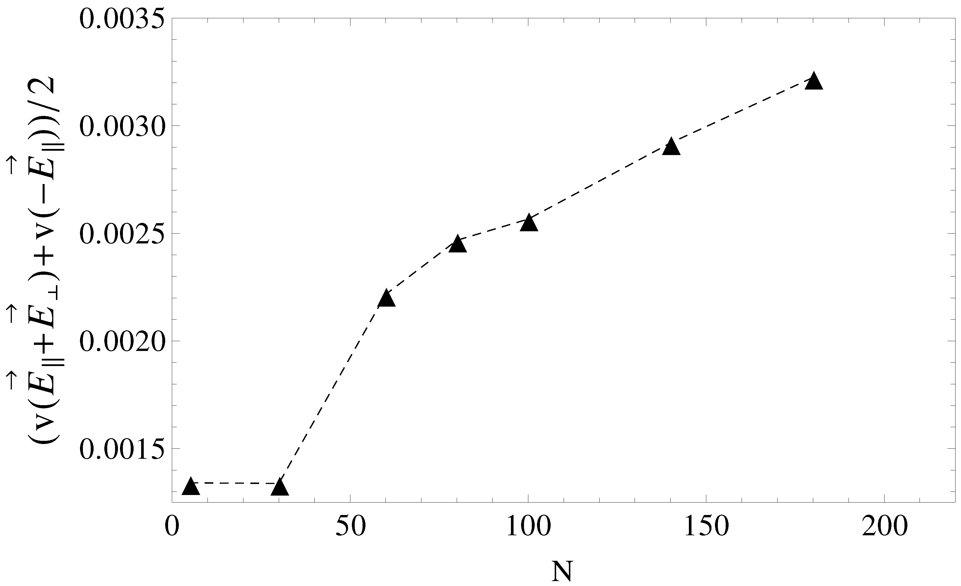
Figure 9.
Average electrophoretic velocities as a function of chain length, N, for the case of pulsed transverse fields and pulsed longitudinal fields. During the first half of the pulse, the driving field is , while in the second half of the pulse, the field is switched to .
Figure 9.
Average electrophoretic velocities as a function of chain length, N, for the case of pulsed transverse fields and pulsed longitudinal fields. During the first half of the pulse, the driving field is , while in the second half of the pulse, the field is switched to .

