Nonlinear Regression Operating on Microstructures Described from Topological Data Analysis for the Real-Time Prediction of Effective Properties


Abstract
1. Introduction
1.1. Model Order Reduction
1.2. Engineered Artificial Intelligence
1.3. Towards Real-Time Decision Making
2. Methods
2.1. Linear Homogenization Procedure
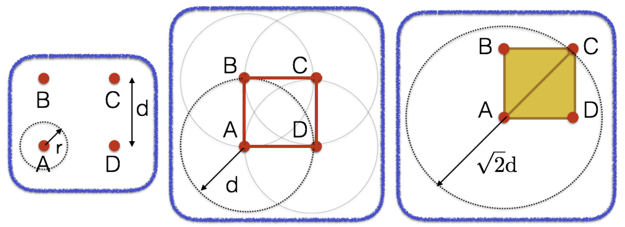
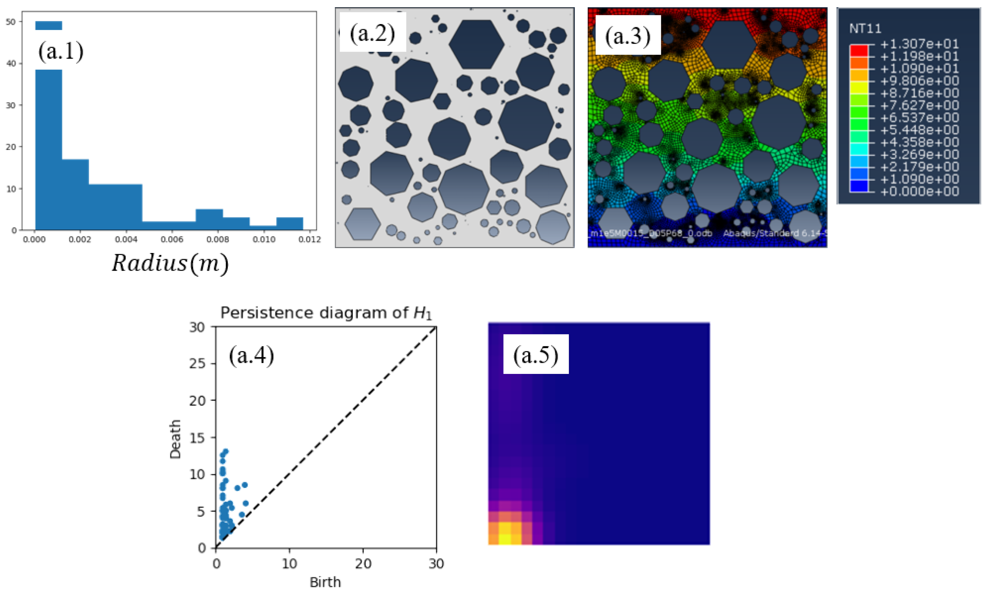
2.2. Topological Data Analysis
2.3. Principal Component Analysis
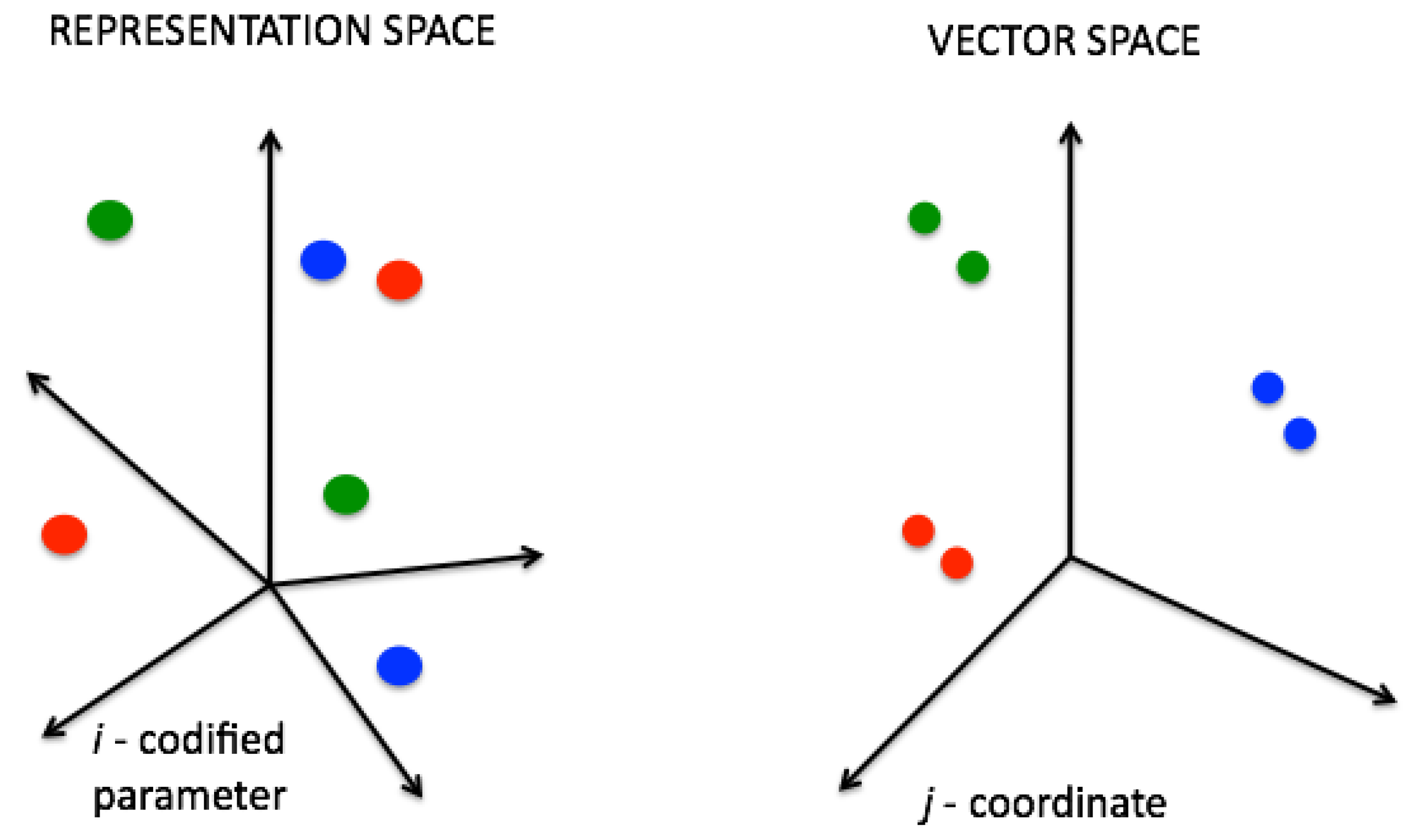
2.4. Code2Vect
3. Results
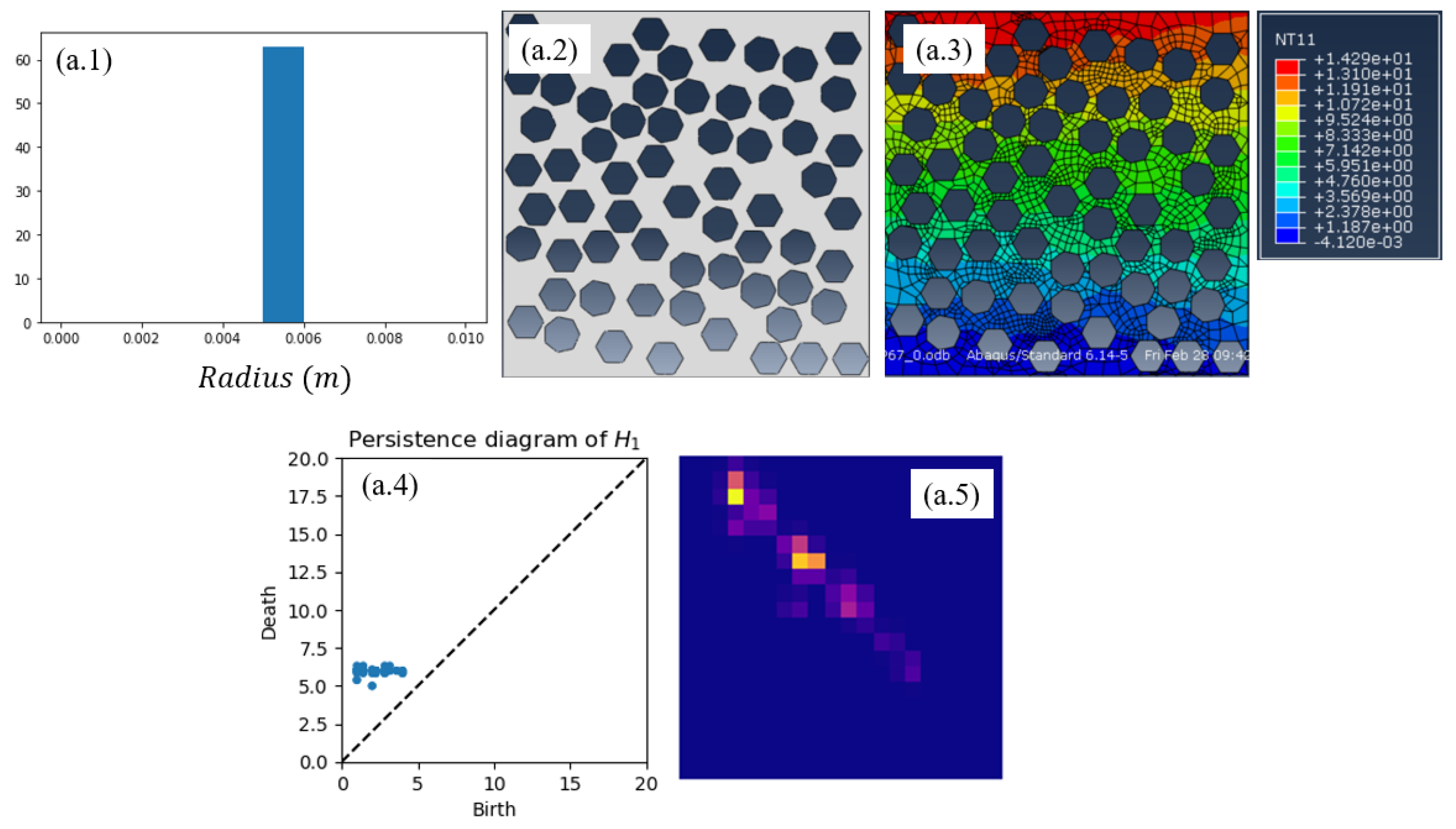
3.1. Model Training
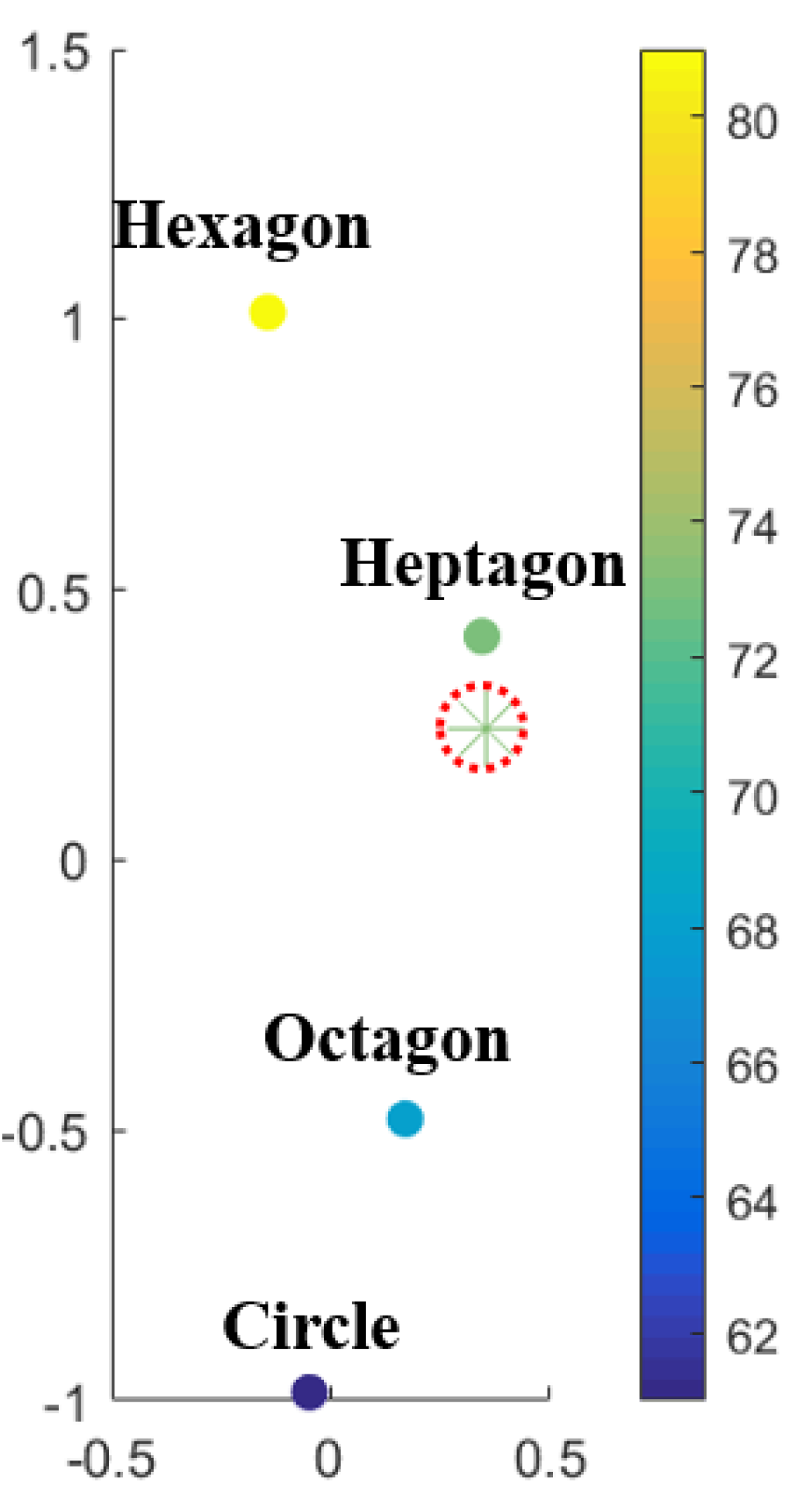
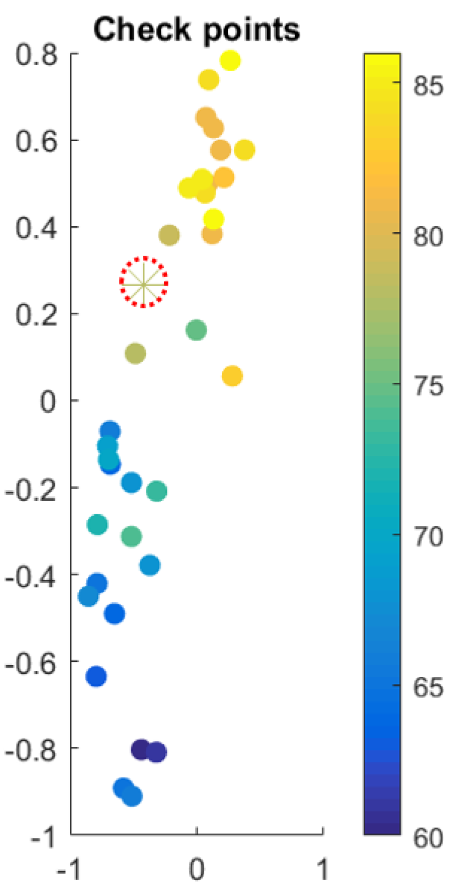
3.2. Inferring Effective Properties
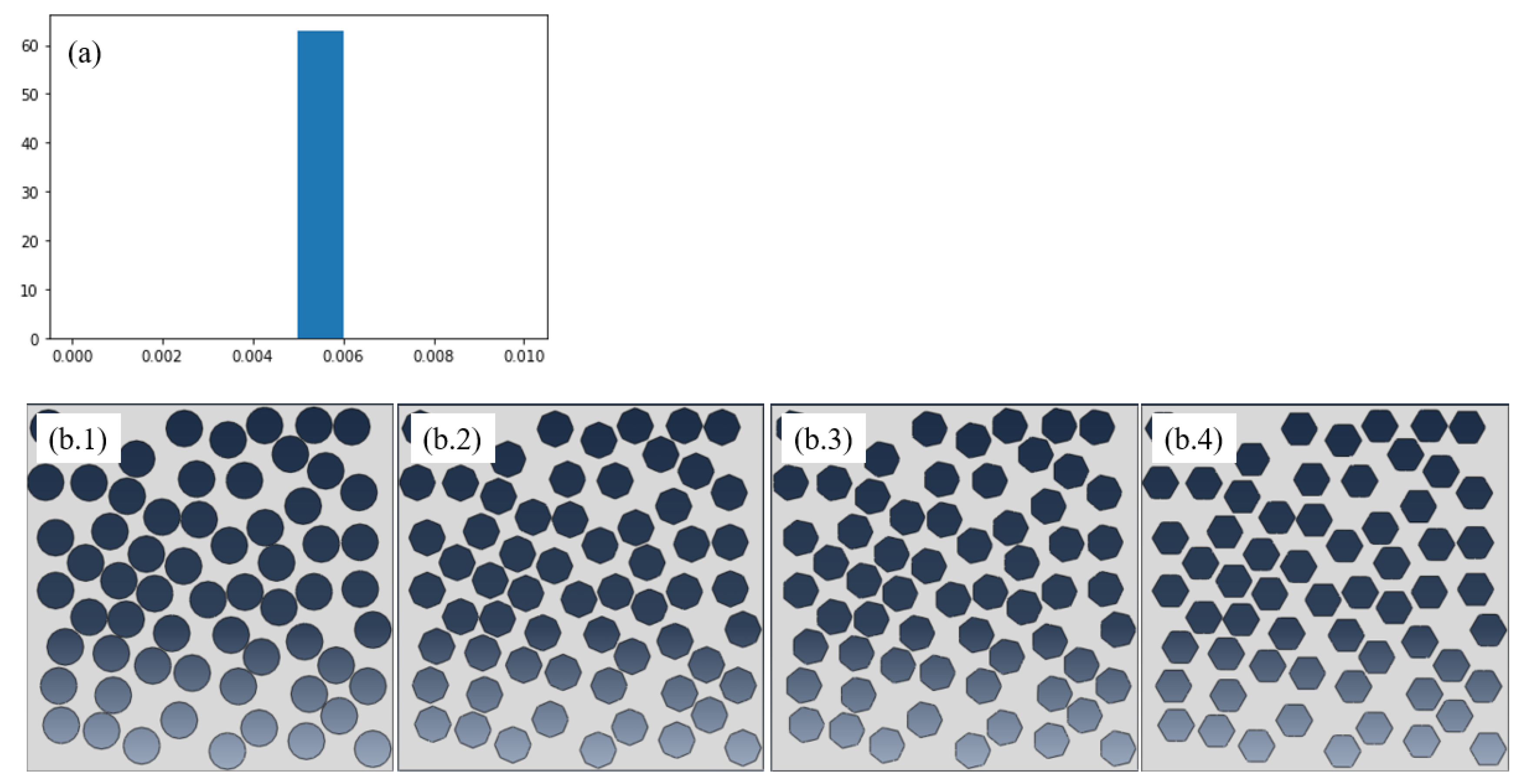
3.3. Microstructures with Varying Shapes and Size Distribution
4. Conclusions
Author Contributions
Funding
Acknowledgments
Conflicts of Interest
References
- Chinesta, F.; Huerta, A.; Rozza, G.; Willcox, K. Model Order Reduction Chapter in the Encyclopedia of Computational Mechanics, 2nd ed.; John Wiley & Sons, Ltd.: Hoboken, NJ, USA, 2015. [Google Scholar]
- Chinesta, F.; Leygue, A.; Bordeu, F.; Aguado, J.V.; Cueto, E.; González, D.; Alfaro, I.; Ammar, A.; Huerta, A. Parametric PGD based computational vademecum for efficient design, optimization and control. Arch. Comput. Methods Eng. 2013, 20, 31–59. [Google Scholar] [CrossRef]
- Chinesta, F.; Keunings, R.; Leygue, A. The Proper Generalized Decomposition for Advanced Numerical Simulations; Springerbriefs, Springer: Berlin, Germany, 2014. [Google Scholar]
- Lee, J.A.; Verleysen, M. Nonlinear Dimensionality Reduction; Springer: New York, NY, USA, 2007. [Google Scholar]
- González, D.; Chinesta, F.; Cueto, E. Thermodynamically consistent data-driven computational mechanics. Continuum Mech. Thermodynamics 2018, 31, 239–253. [Google Scholar] [CrossRef]
- González, D.; Cueto, E.; Chinesta, F. Computational patient avatars for surgery planning. Ann. Biomed. Eng. 2016, 44, 35–45. [Google Scholar] [CrossRef] [PubMed]
- Lopez, E.; Gonzalez, D.; Aguado, J.V.; Abisset-Chavanne, E.; Cueto, E.; Binetruy, C.; Chinesta, F. A manifold learning approach for integrated computational materials engineering. Arch. Comput. Methods Eng. 2016, 25, 59–68. [Google Scholar] [CrossRef]
- Gonzalez, D.; Aguado, J.V.; Cueto, E.; Abisset-Chavanne, E.; Chinesta, F. kPCA-based Parametric Solutions within the PGD Framework. Arch. Comput. Methods Eng. 2018, 25, 69–86. [Google Scholar] [CrossRef]
- Maaten, L.; Hinton, G. Visualizing data using t-SNE. J. Mach. Learn. Res. 2008, 9, 2579–2605. [Google Scholar]
- Cristianini, N.; Shawe-Taylor, J. An Introduction to Support Vector Machines: And Other Kernel-Based Learning Methods; Cambridge University Press: New York, NY, USA, 2000. [Google Scholar]
- Forgy, E. Cluster analysis of multivariate data: Efficiency versus interpretability of classification. Biometrics 1965, 21, 768–769. [Google Scholar]
- Ibanez, R.; Abisset-Chavanne, E.; Ammar, A.; Gonzalez, D.; Cueto, E.; Huerta, A.; Duval, J.L.; Chinesta, F. A multi-dimensional data-driven sparse identification technique: The sparse Proper Generalized Decomposition. Complexity 2018, 5608286. [Google Scholar] [CrossRef]
- Argerich, C.; Ibanez, R.; Barasinski, A.; Chinesta, F. Code2vect: An efficient heterogenous data classifier and nonlinear regression technique. Comptes Rendus Mécanique 2019, 347, 754–761. [Google Scholar] [CrossRef]
- Reille, A.; Hascoet, N.; Ghnatios, C.; Ammar, A.; Cueto, E.; Duval, J.L.; Chinesta, F.; Keunings, R. Incremental dynamic mode decomposition: A reduced-model learner operating at the low-data limit. Comptes Rendus Mécanique 2019, 347, 780–792. [Google Scholar] [CrossRef]
- Schmid, P.J. Dynamic mode decomposition of numerical and experimental data. J. Fluid Mech. 2010, 656, 5–28. [Google Scholar] [CrossRef]
- Williams, M.O.; Kevrekidis, G.; Rowley, C.W. A data-driven approximation of the Koopman operator: Extending dynamic mode decomposition. J. Nonlinear Sci. 2015, 25, 1307–1346. [Google Scholar] [CrossRef]
- Goodfellow, I.; Bengio, Y.; Courville, A. Deep Learning; MIT Press: Cambridge, UK, 2016. [Google Scholar]
- Moya, B.; Gonzalez, D.; Alfaro, I.; Chinesta, F.; Cueto, E. Learning slosh dynamics by means of data. Comput. Mech. 2019, 64, 511–523. [Google Scholar] [CrossRef]
- Chinesta, F.; Cueto, E.; Abisset-Chavanne, E.; Duval, J.L.; El Khaldi, F. Virtual, Digital and Hybrid Twins: A New Paradigm in Data-Based Engineering and Engineered Data. Arch. Comput. Methods Eng. 2020, 27, 105–134. [Google Scholar] [CrossRef]
- González, D.; Chinesta, F.; Cueto, E. Learning corrections for hyperelastic models from data. Front. Mater. Comput. Mater. Sci. 2019, 6. [Google Scholar] [CrossRef]
- Wasserman, L. Topological data analysis. Ann. Rev. Stat. Appl. 2018, 5, 501–532. [Google Scholar] [CrossRef]
- Lamari, H.; Ammar, A.; Cartraud, P.; Legrain, G.; Jacquemin, F.; Chinesta, F. Routes for Efficient Computational Homogenization of Non-Linear Materials Using the Proper Generalized Decomposition. Arch. Comput. Methods Eng. 2010, 17, 373–391. [Google Scholar] [CrossRef]
- Adams, H.; Emerson, T.; Kirby, M.; Neville, R.; Peterson, C.; Shipman, P.; Chepushtanova, S.; Hanson, E.; Motta, F.; Ziegelmeier, L. Persistence images: A stable vector representation of persistent homology. J. Mach. Learn. Res. 2017, 18, 218–252. [Google Scholar]


| Number of Samples | Relative Error |
|---|---|
| 13 | 0.076 |
| 16 | 0.056 |
| 19 | 0.046 |
| 35 | 0.037 |
© 2020 by the authors. Licensee MDPI, Basel, Switzerland. This article is an open access article distributed under the terms and conditions of the Creative Commons Attribution (CC BY) license (http://creativecommons.org/licenses/by/4.0/).
Share and Cite
Yun, M.; Argerich, C.; Cueto, E.; Duval, J.L.; Chinesta, F. Nonlinear Regression Operating on Microstructures Described from Topological Data Analysis for the Real-Time Prediction of Effective Properties. Materials 2020, 13, 2335. https://doi.org/10.3390/ma13102335
Yun M, Argerich C, Cueto E, Duval JL, Chinesta F. Nonlinear Regression Operating on Microstructures Described from Topological Data Analysis for the Real-Time Prediction of Effective Properties. Materials. 2020; 13(10):2335. https://doi.org/10.3390/ma13102335
Chicago/Turabian StyleYun, Minyoung, Clara Argerich, Elias Cueto, Jean Louis Duval, and Francisco Chinesta. 2020. "Nonlinear Regression Operating on Microstructures Described from Topological Data Analysis for the Real-Time Prediction of Effective Properties" Materials 13, no. 10: 2335. https://doi.org/10.3390/ma13102335
APA StyleYun, M., Argerich, C., Cueto, E., Duval, J. L., & Chinesta, F. (2020). Nonlinear Regression Operating on Microstructures Described from Topological Data Analysis for the Real-Time Prediction of Effective Properties. Materials, 13(10), 2335. https://doi.org/10.3390/ma13102335