Numerical Study on Transient State of Inductive Fault Current Limiter Based on Field-Circuit Coupling Method


Abstract
:1. Introduction
2. Methodology of Numerical Model
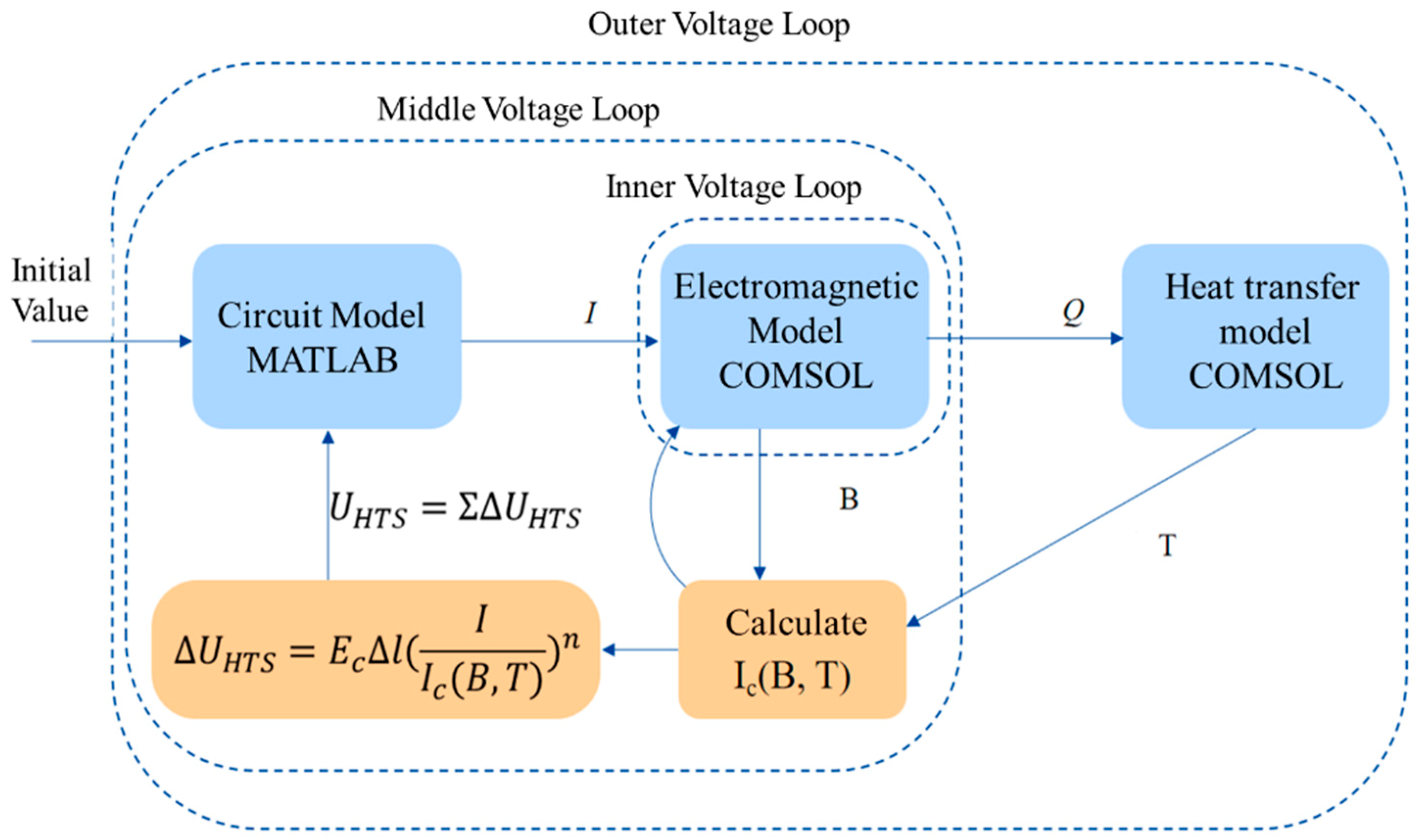
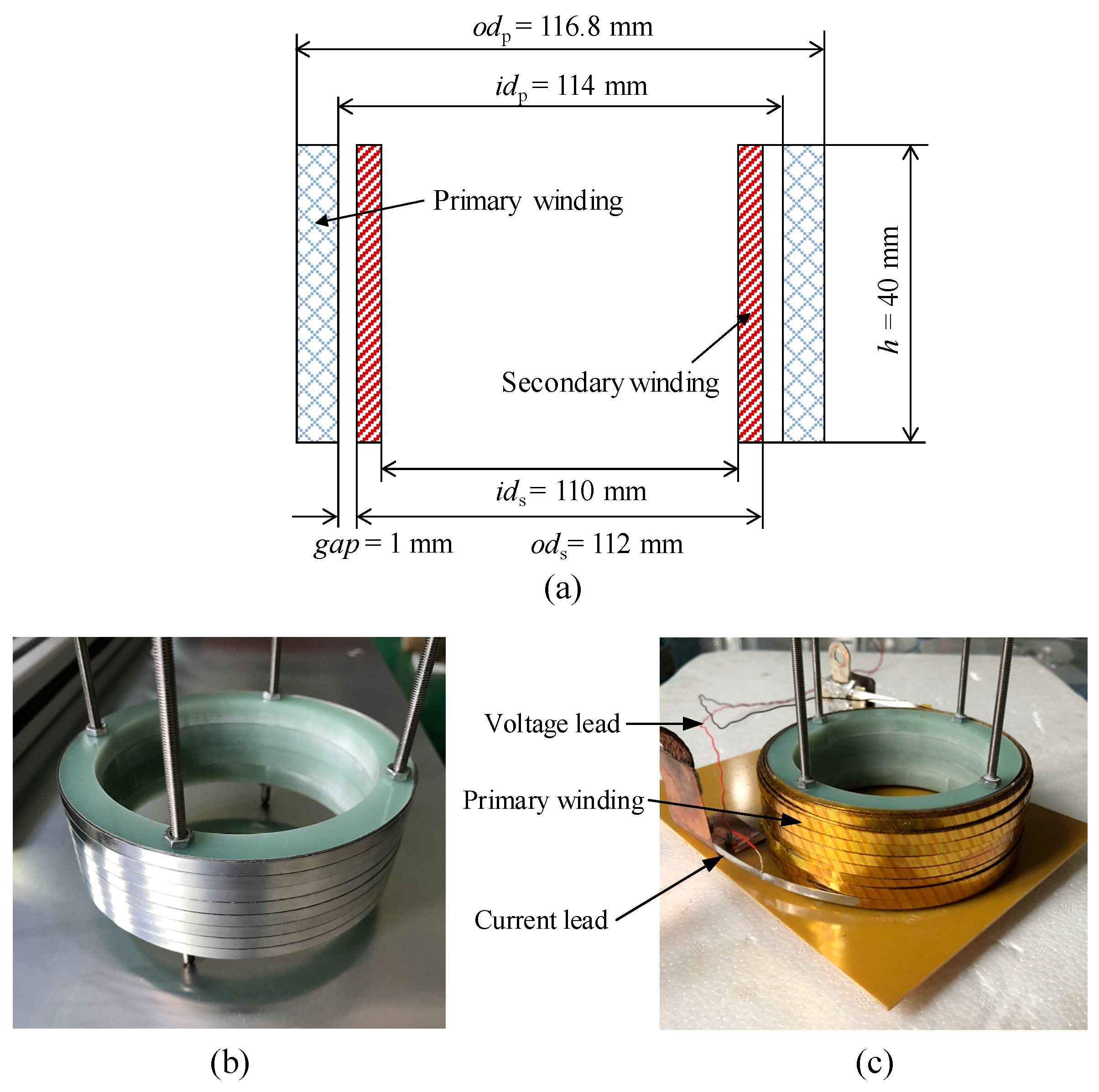
2.1. Model Overview
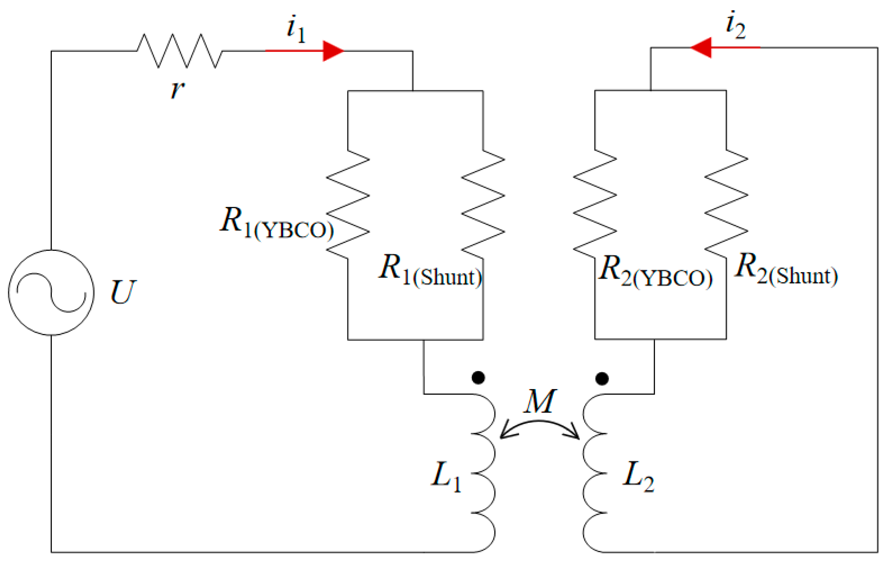
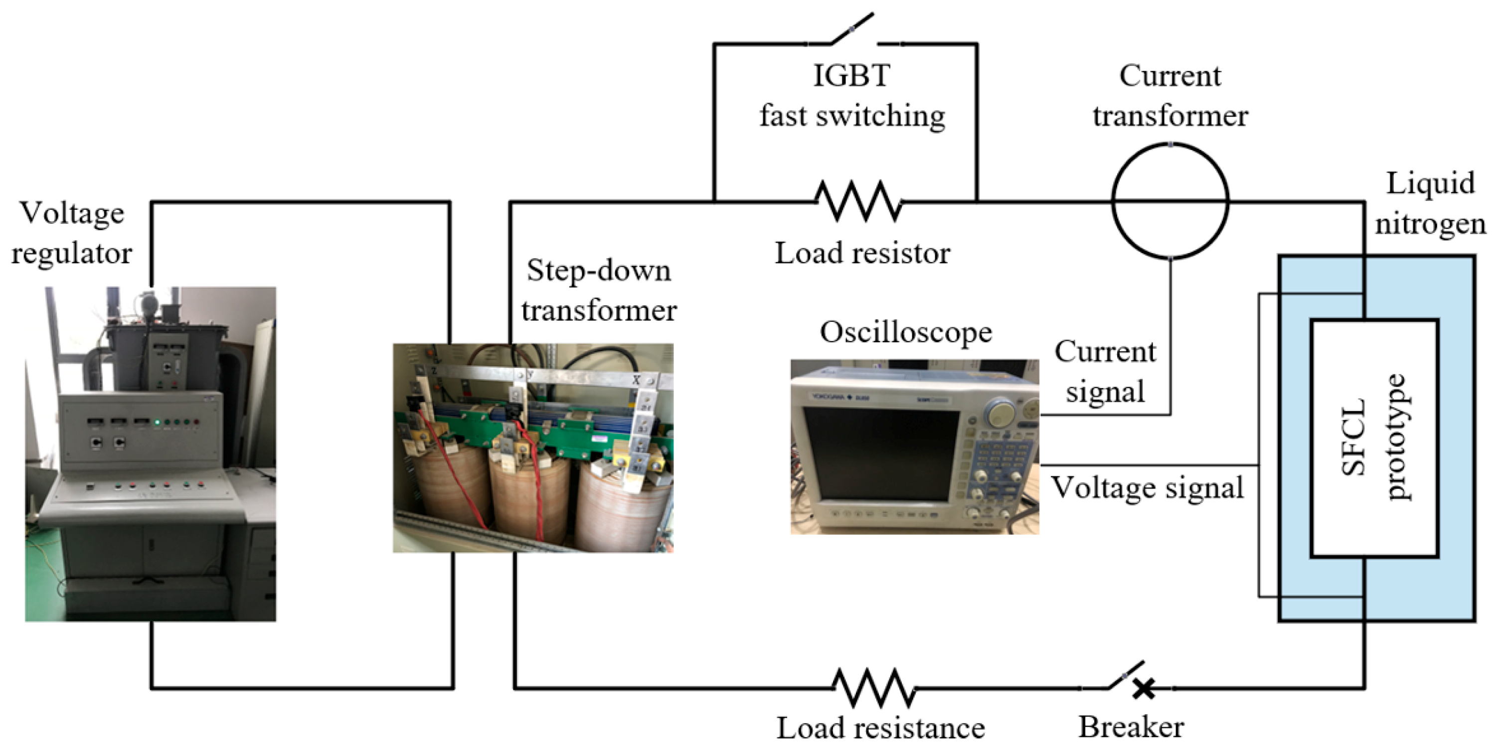
2.2. Circuit Model
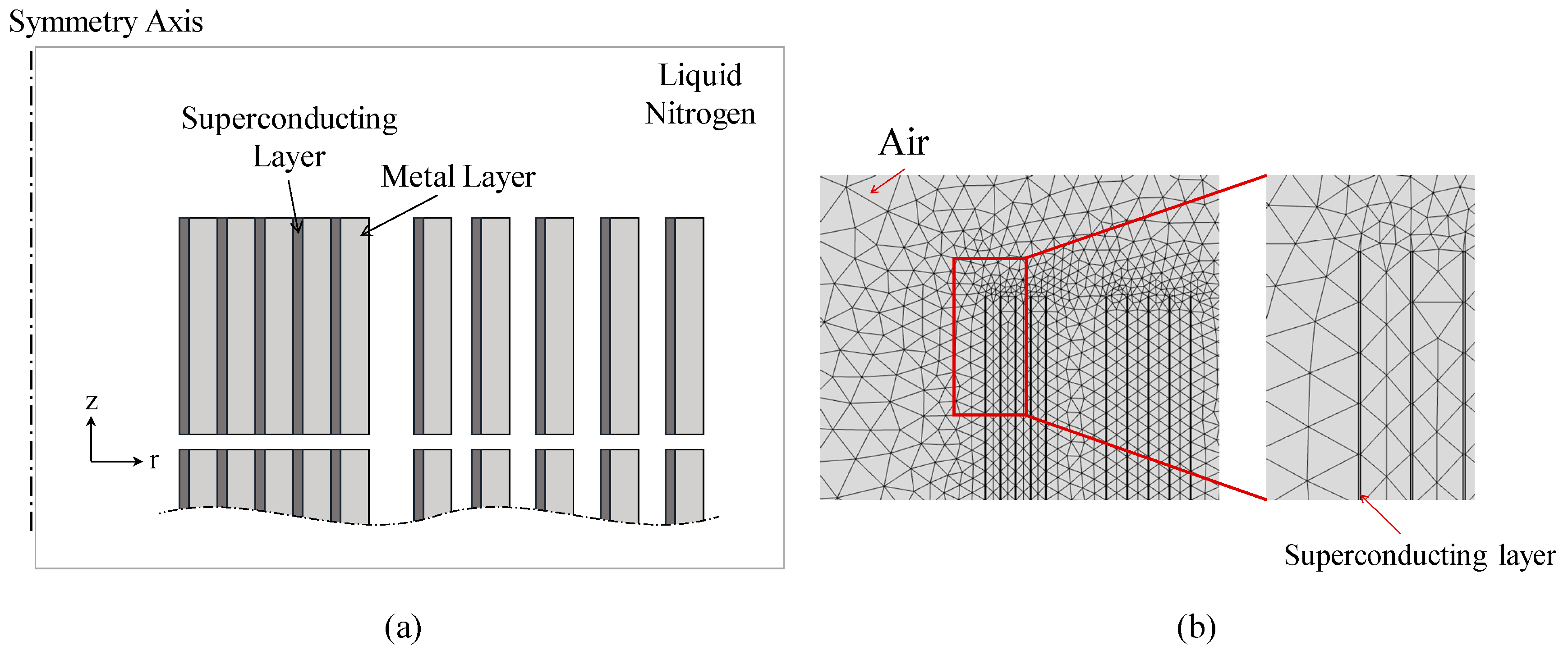
2.3. Electromagnetic Model
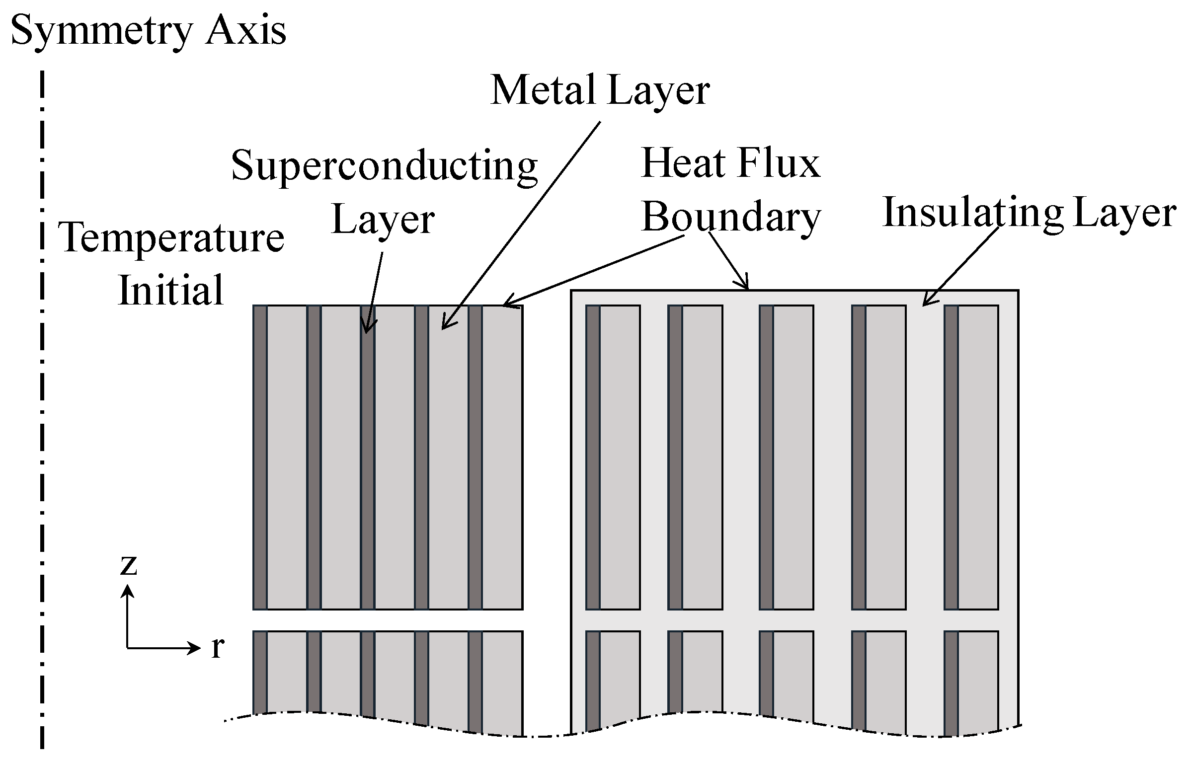
2.4. Heat Transfer Model
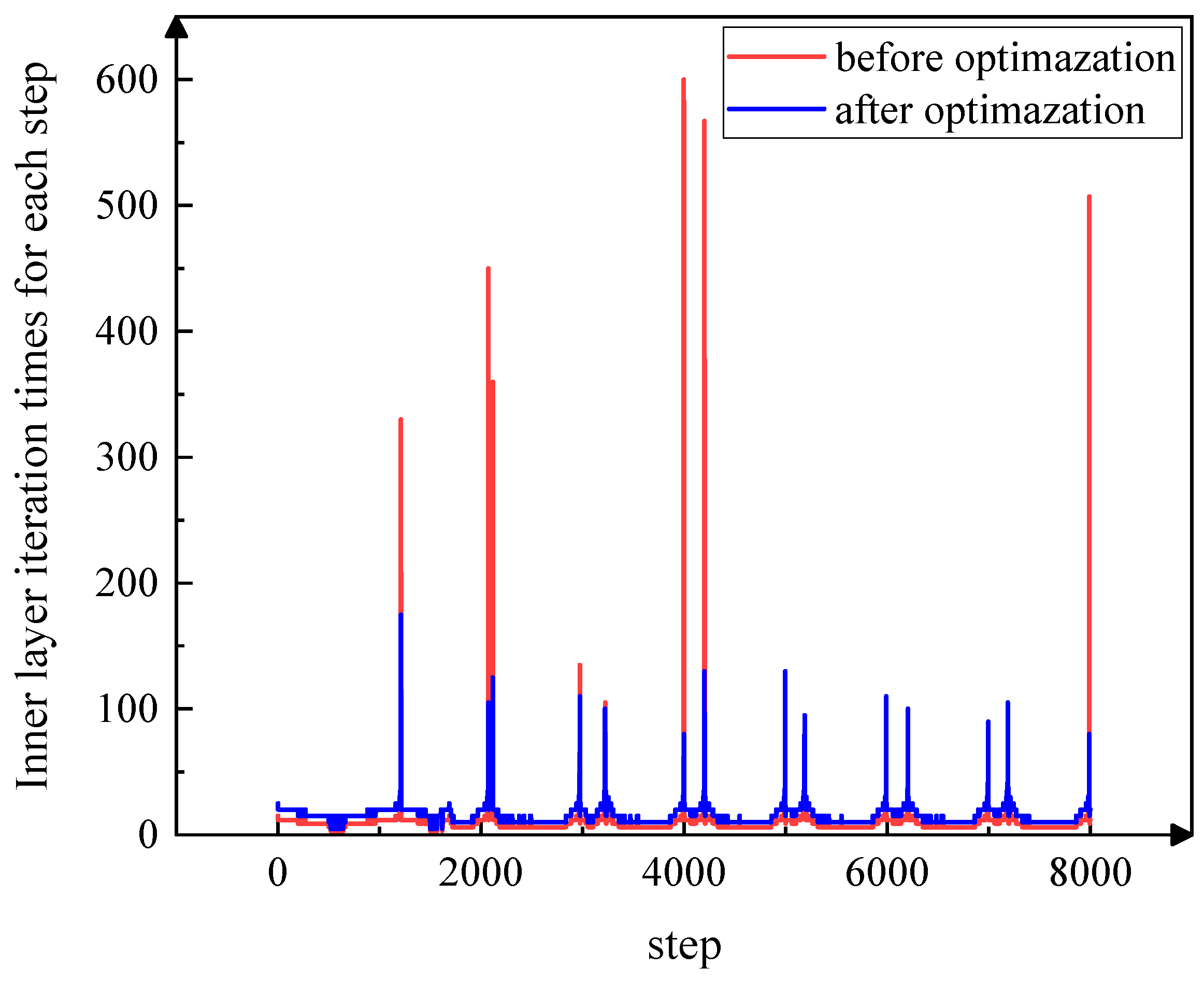
2.5. Model Convergence and Optimization
2.5.1. Middle Voltage Loop Optimization
2.5.2. Inner Voltage Loop Optimization
3. Results and Discussion
3.1. Typical Examples
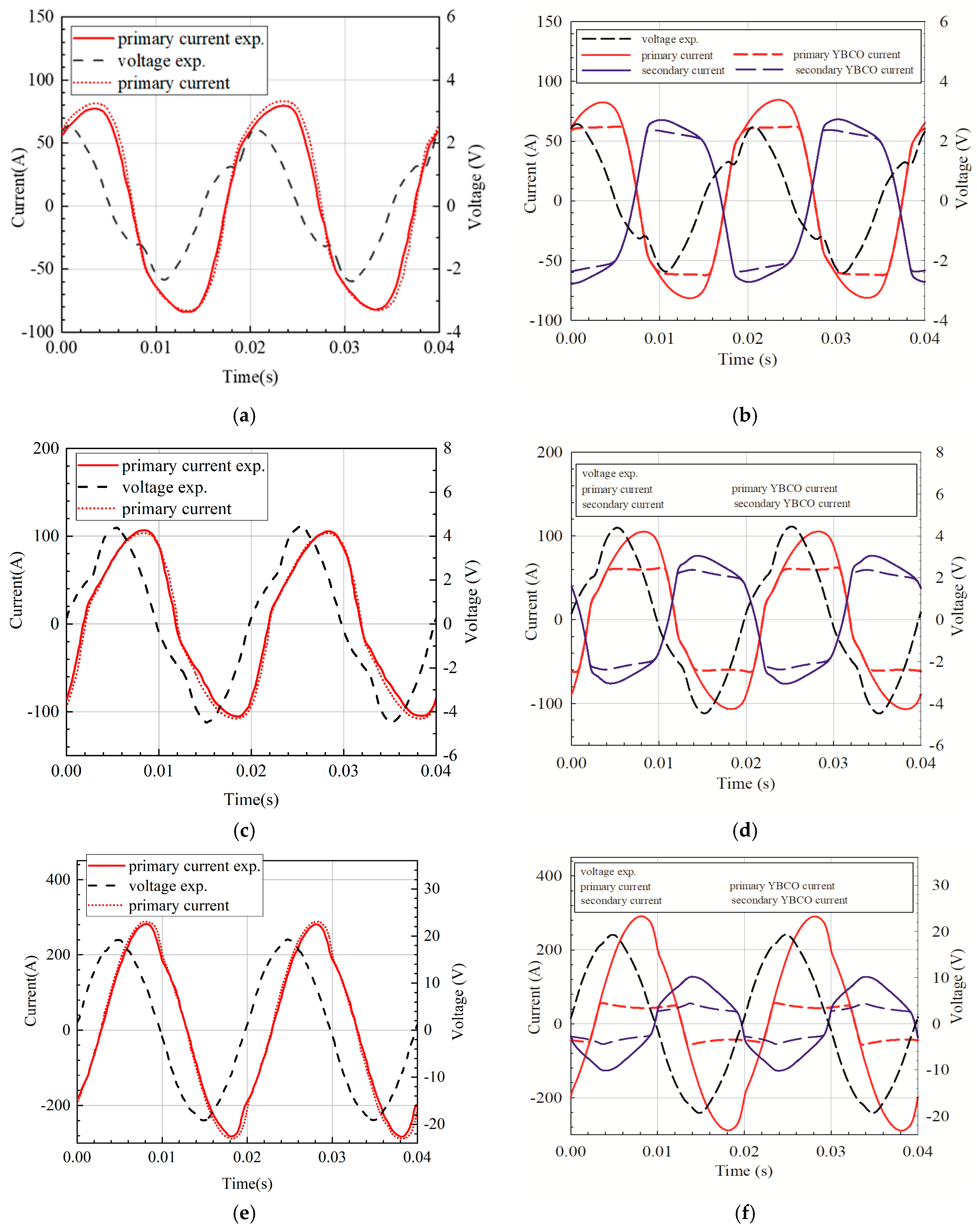
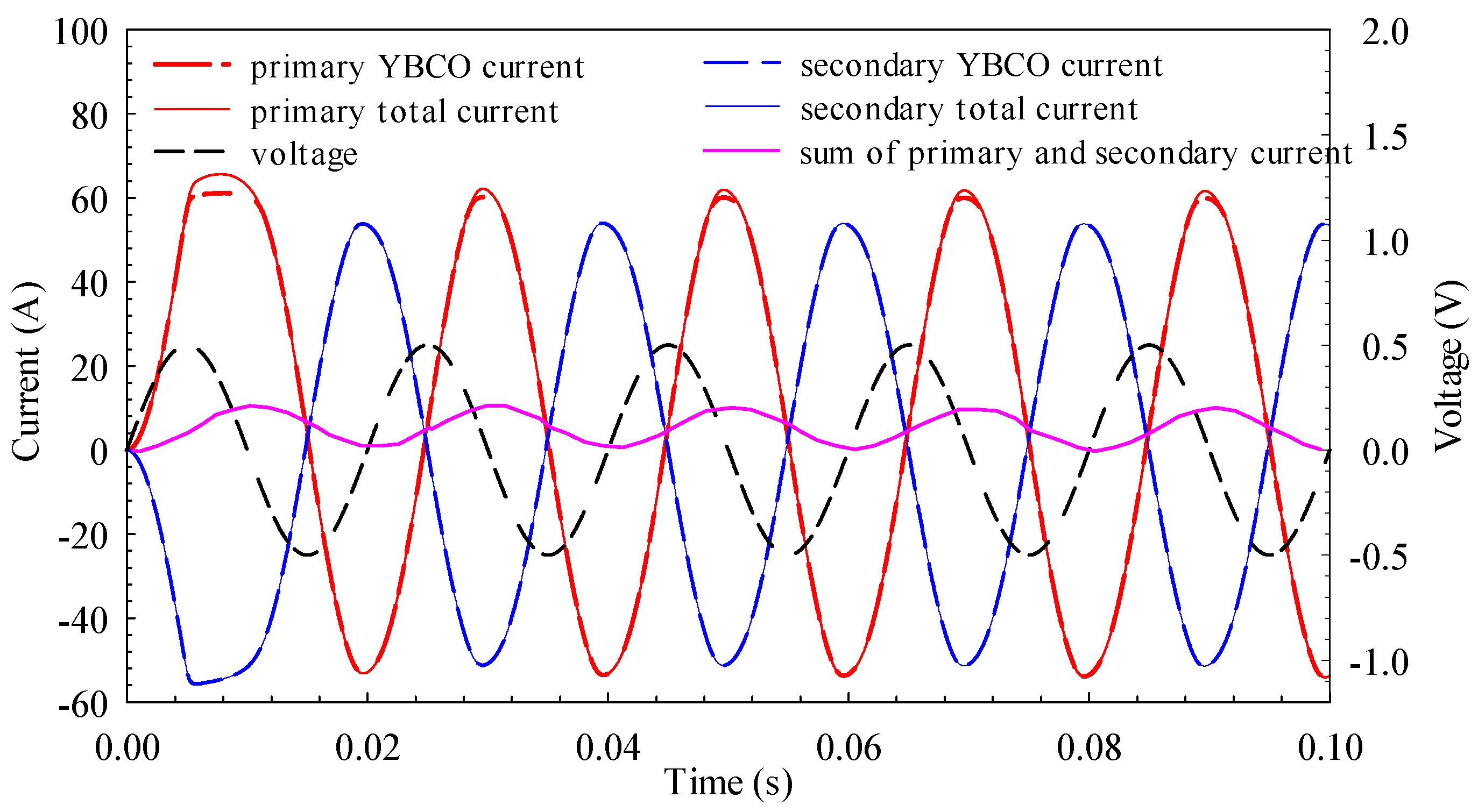
3.1.1. Current and Voltage
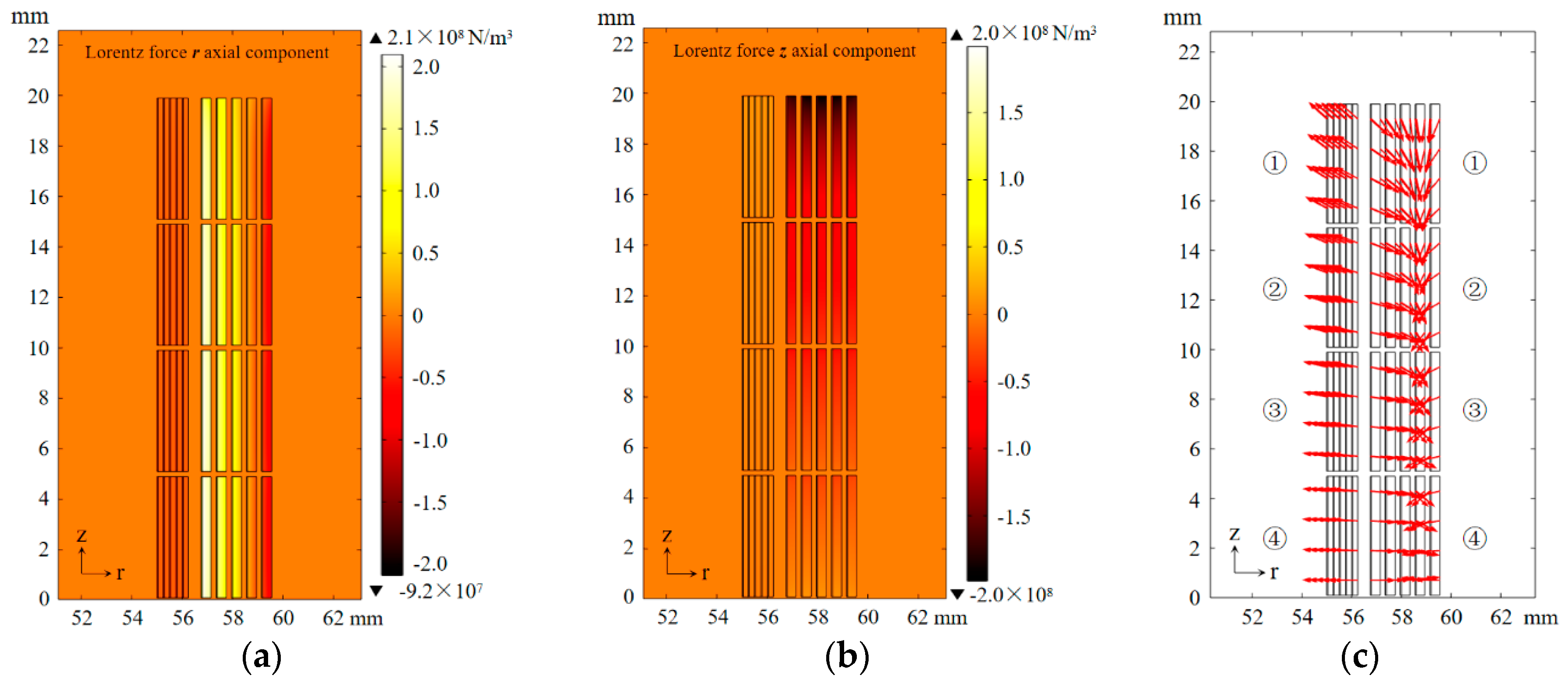
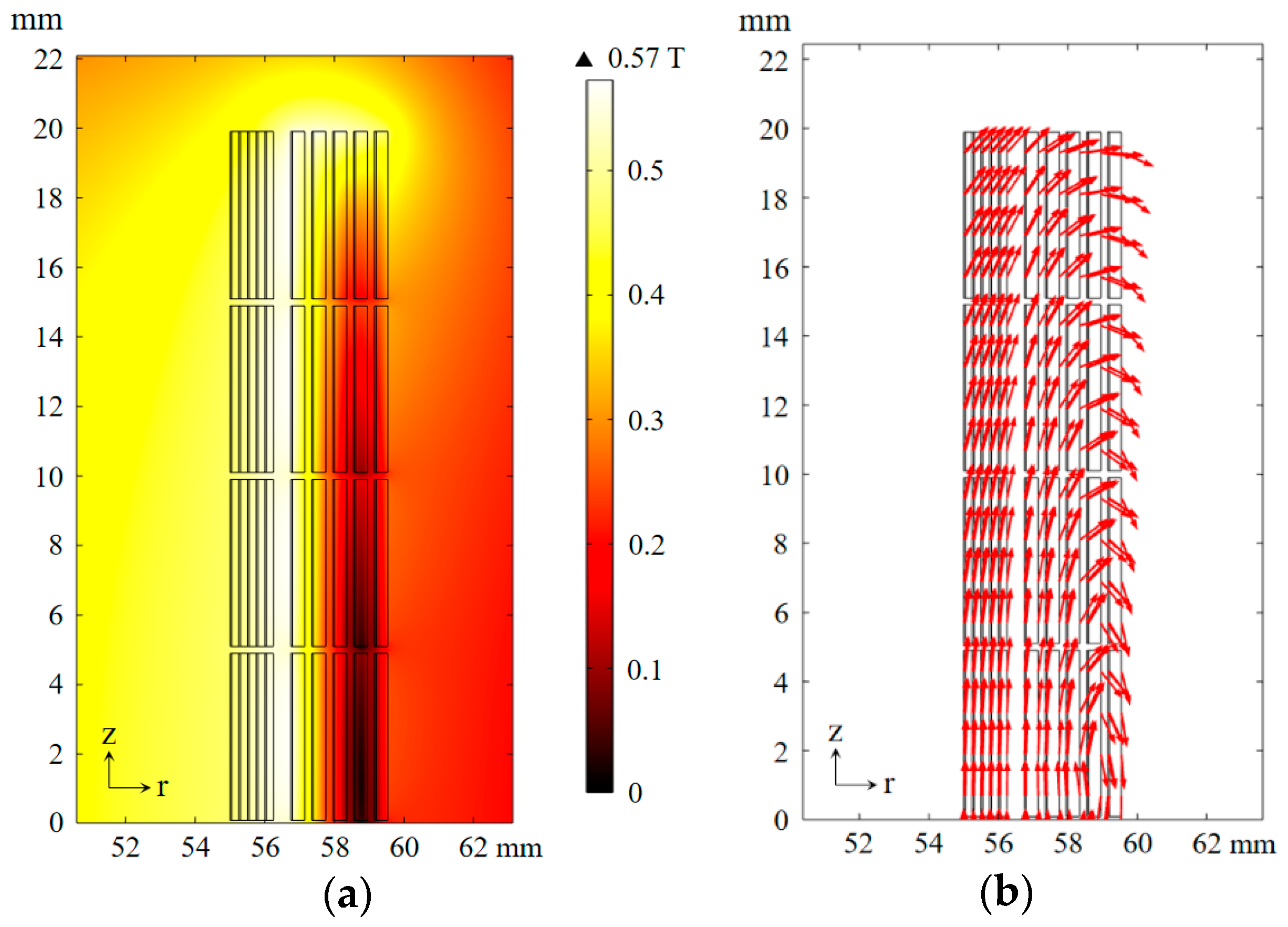
3.1.2. Magnetic Field and Electrodynamic Force
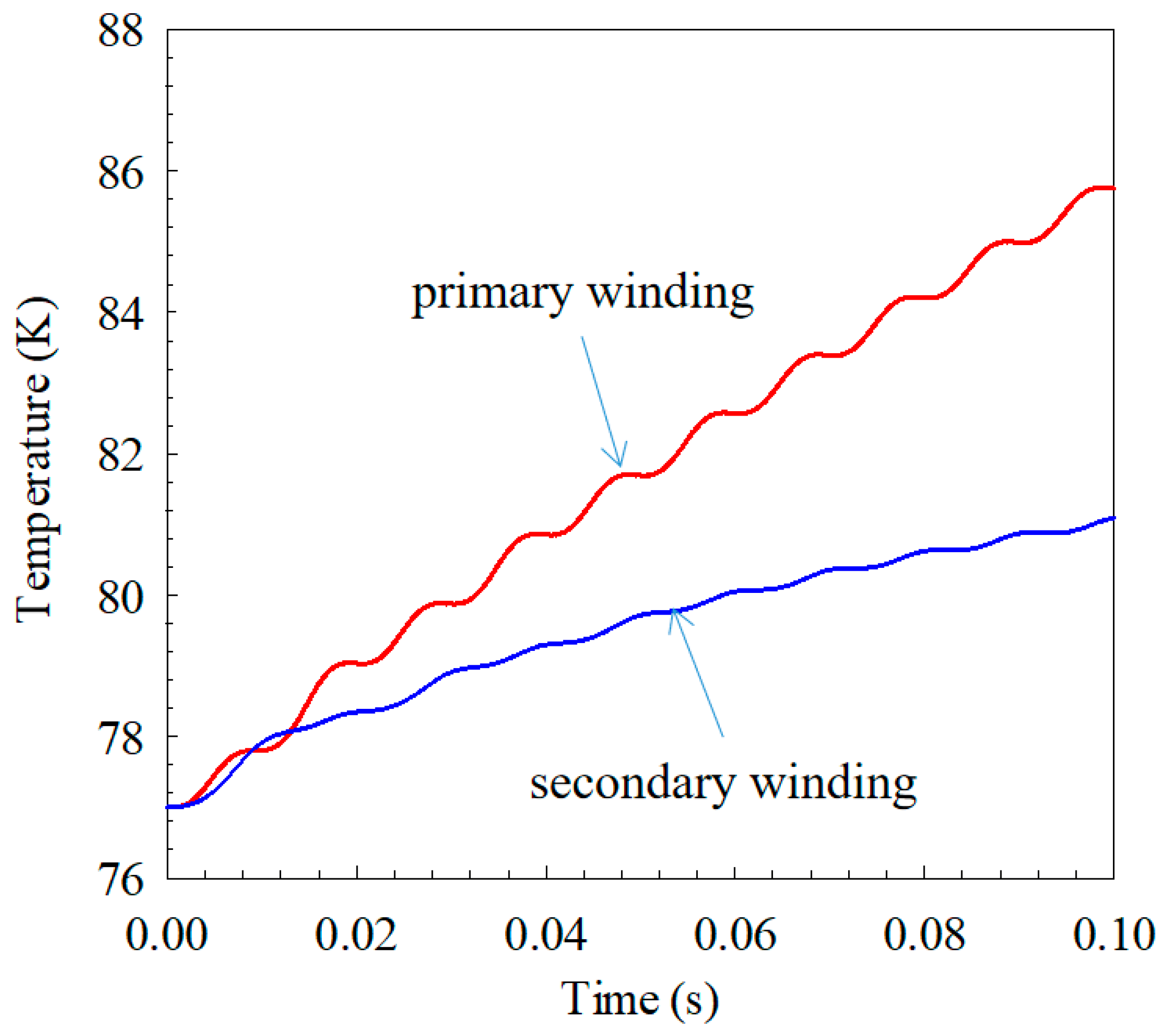
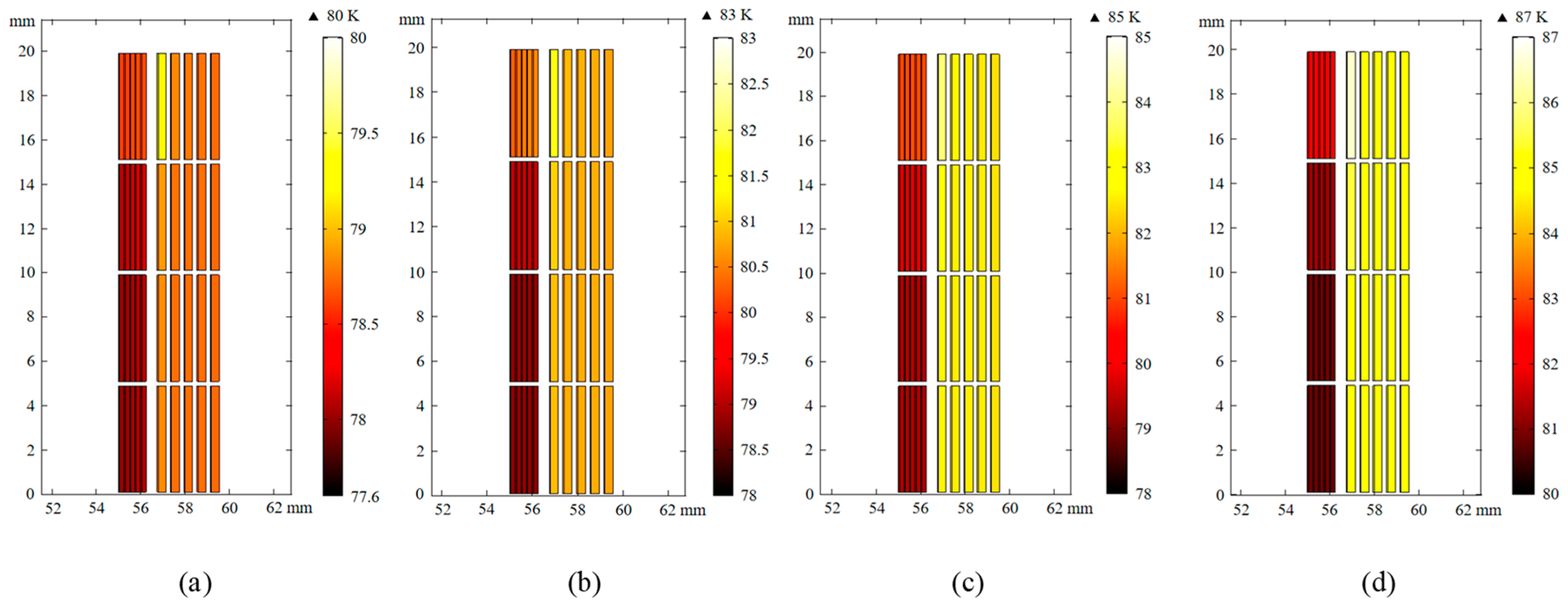
3.1.3. Temperature
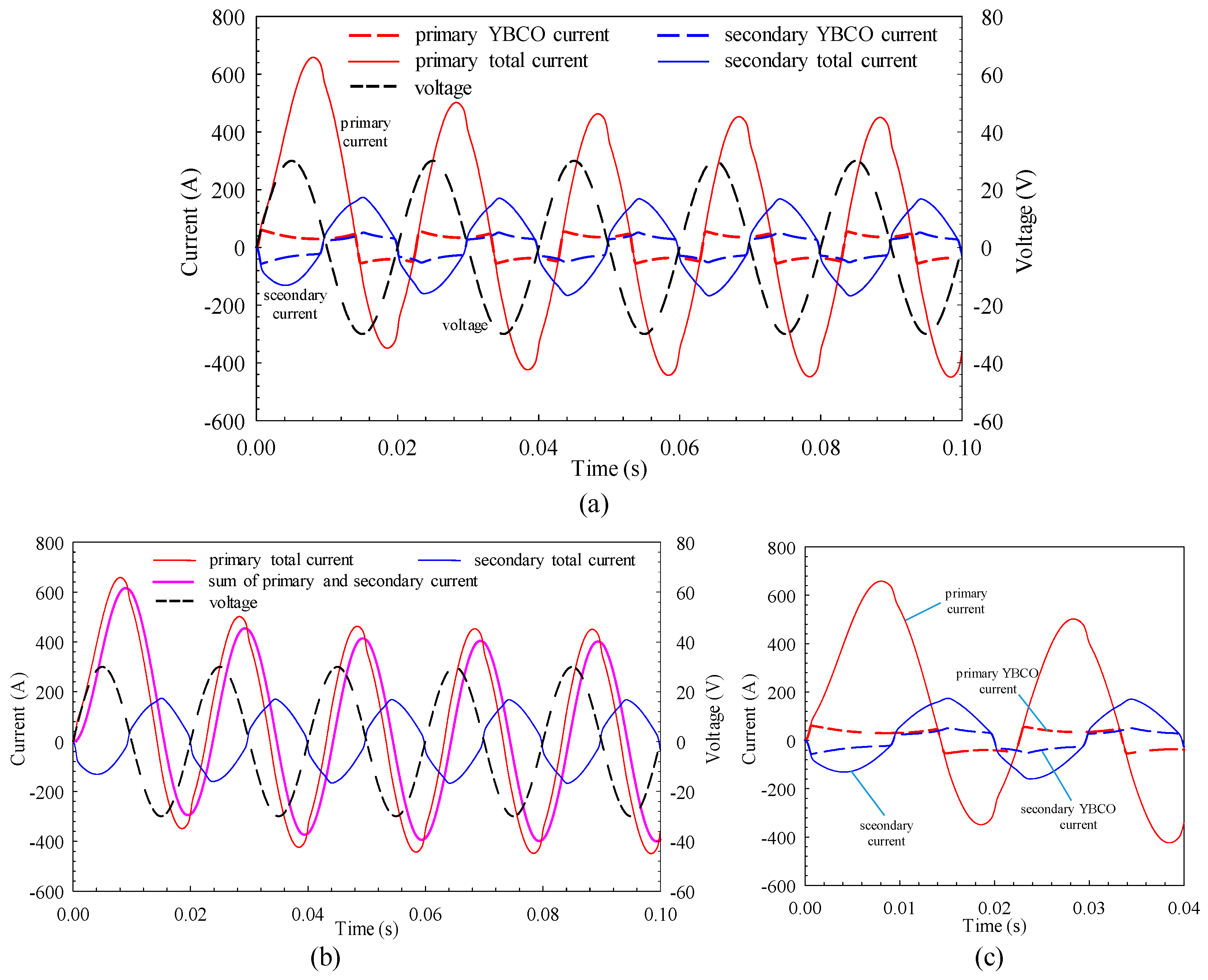
3.2. Short-Circuit Test
4. Conclusions
Author Contributions
Funding
Conflicts of Interest
References
- Ruiz, H.S.; Zhang, X.; Coombs, T.A. Resistive-type superconducting fault current limiters: Concepts, materials, and numerical modeling. IEEE Trans. Appl. Supercond. 2015, 25, 5601405. [Google Scholar] [CrossRef]
- Naeckel, O.; Noe, M. Design and Test of an Air Coil Superconducting Fault Current Limiter Demonstrator. IEEE Trans. Appl. Supercond. 2014, 24, 5601605. [Google Scholar] [CrossRef]
- Meerovich, V.; Sokolovsky, V.; Bock, J.; Gauss, S.; Goren, S.; Jung, G. Performance of an inductive fault current limiter employing BSCCO superconducting cylinders. IEEE Trans. Appl. Supercond. 1999, 9, 4666–4676. [Google Scholar] [CrossRef]
- Usoskin, A.; Mumford, F.; Dietrich, R.; Handaze, A.; Prause, B.; Rutt, A.; Schlenga, K. Inductive Fault Current Limiters: Kinetics of Quenching and Recovery. IEEE Trans. Appl. Supercond. 2009, 19, 1859–1862. [Google Scholar] [CrossRef]
- Kozak, J.; Majka, M.; Kozak, S.; Janowski, T. Design and tests of coreless inductive superconducting fault current limiter. IEEE Trans. Appl. Supercond. 2012, 22, 5601804. [Google Scholar] [CrossRef]
- Paul, W.; Lakner, M.; Rhyner, J.; Unternährer, P.; Baumann, T.; Chen, M.; Guerig, A. Test of 1.2 MVA high-superconducting fault current limiter. Supercond. Sci. Technol. 1997, 10, 914–918. [Google Scholar] [CrossRef]
- Kozak, J.; Majka, M.; Kozak, S. Experimental Results of a 15 kV, 140 A Superconducting Fault Current Limiter. IEEE Trans. Appl. Supercond. 2017, 27, 5600504. [Google Scholar] [CrossRef]
- Cvoric, D.; De Haan, S.W.H.; Ferreira, J.A.; Van Riet, M.; Bozelie, J. Design and Testing of Full-Scale 10 kV Prototype of Inductive Fault Current Limiter with a Common Core and Trifilar Windings. In Proceedings of the 2010 International Conference on Electrical Machines and Systems, Incheon, South Korea, 10–13 October 2010. [Google Scholar]
- Hong, Z.; Campbell, A.M.; Coombs, T.A. Numerical solution of critical state in superconductivity by finite element software. Supercond. Sci. Technol. 2006, 19, 1246–1252. [Google Scholar] [CrossRef]
- Hong, Z.; Coombs, T.A. Numerical Modelling of AC Loss in Coated Conductors by Finite Element Software Using H Formulation. J. Supercond. Nov. Magn. 2010, 23, 1551–1562. [Google Scholar] [CrossRef]
- Zhang, H.; Zhang, M.; Yuan, W. An efficient 3D finite element method model based on the T–A formulation for superconducting coated conductors. Supercond. Sci. Technol. 2017, 30, 024005. [Google Scholar] [CrossRef]
- Wang, Y.; Zhang, M.; Grilli, F.; Zhu, Z.; Yuan, W. Study of the magnetization loss of CORC cables using 3D TA formulation. Supercond. Sci. Technol. 2019, 32, 025003. [Google Scholar] [CrossRef]
- Kozak, S.; Janowski, T.; Wojtasiewicz, G.; Kozak, J.; Kondratowicz-Kucewicz, B.; Majka, M. The 15 kV Class Inductive SFCL. IEEE Trans. Appl. Supercond. 2010, 20, 1203–1206. [Google Scholar] [CrossRef]
- Naeckel, O.; Noe, M. Conceptual Design Study of an Air Coil Fault Current Limiter. IEEE Trans. Appl. Supercond. 2013, 23, 5602404. [Google Scholar] [CrossRef]
- Hekmati, A.; Vakilian, M.; Fardmanesh, M. Flux-Based Modeling of Inductive Shield-Type High-Temperature Superconducting Fault Current Limiter for Power Networks. IEEE Trans. Appl. Supercond. 2011, 21, 3458–3464. [Google Scholar] [CrossRef]
- Kado, H.; Ichikawa, M.; Ueda, H.; Ishiyama, A. Trial Design of 6.6kV Magnetic Shielding Type of Superconducting Fault Current Limiter and Performance Analysis Based on Finite Element Method. Electr. Eng. Jpn. 2010, 145, 50–57. [Google Scholar] [CrossRef]
- Sheng, J.; Wen, J.; Wei, Y.; Zeng, W.; Jin, Z.; Hong, Z. Voltage-Source Finite-Element Model of High Temperature Superconducting Tapes. IEEE Trans. Appl. Supercond. 2015, 25, 7200305. [Google Scholar] [CrossRef]
- Sheng, J.; Hu, D.; Ryu, K.; Yang, H.S.; Li, Z.Y.; Hong, Z. Numerical Study on Overcurrent Process of High-Temperature Superconducting Coated Conductors. J. Supercond. Nov. Magn. 2017, 30, 3263–3270. [Google Scholar] [CrossRef]
- Grilli, F.; Sirois, F.; Zermeno, V.M.R.; Vojenciak, M. Selfconsistent modeling of the Ic of HTS devices: How accurate do models really need to be? IEEE Trans. Appl. Supercond. 2014, 24, 8000508. [Google Scholar] [CrossRef]
- Wang, Y.; Chan, W.K.; Schwartz, J. Self-protection mechanisms in no-insulation (RE)Ba2Cu3Ox, high temperature superconductor pancake coils. Supercond. Sci. Technol. 2016, 29, 045007. [Google Scholar] [CrossRef]
- Sakurai, A.; Shiotsu, M.; Hata, K. Boiling heat transfer characteristics for heat inputs with various increasing rates in liquid nitrogen. Cryogenics 1992, 32, 421–429. [Google Scholar] [CrossRef]


| Item | Specifications | Value |
|---|---|---|
| YBCO tape | Tape width | 4.8 mm |
| Thickness without insulation | 0.25 mm | |
| Ic/n-value (@77 K, self-field) | 40 A/29 | |
| Critical temperature | 92 K | |
| Primary winding (insulation) | Number of turns | 40 |
| Inner/outer diameter | 114 mm/116.8 mm | |
| Turn-to-turn gap | 0.35 mm | |
| Secondary winding (no-insulation) | Number of turns | 40 |
| Inner/outer diameter | 110 mm/112 mm | |
| Turn-to-turn gap | 0.25 mm |
| Primary Winding | Secondary Winding | |
|---|---|---|
| No. | Electrodynamic force r-axial component (N/m) | |
| 1 | 438.3 | −116.6 |
| 2 | 493.4 | −138.6 |
| 3 | 517.7 | −144.9 |
| 4 | 528.4 | −147.1 |
| No. | Electrodynamic force z-axial component (N/m) | |
| 1 | −1023.4 | 75.9 |
| 2 | −535.8 | 45.8 |
| 3 | −283.8 | 24.7 |
| 4 | −89.9 | 7.9 |
© 2019 by the authors. Licensee MDPI, Basel, Switzerland. This article is an open access article distributed under the terms and conditions of the Creative Commons Attribution (CC BY) license (http://creativecommons.org/licenses/by/4.0/).
Share and Cite
Li, W.; Sheng, J.; Qiu, D.; Cheng, J.; Ye, H.; Hong, Z. Numerical Study on Transient State of Inductive Fault Current Limiter Based on Field-Circuit Coupling Method. Materials 2019, 12, 2805. https://doi.org/10.3390/ma12172805
Li W, Sheng J, Qiu D, Cheng J, Ye H, Hong Z. Numerical Study on Transient State of Inductive Fault Current Limiter Based on Field-Circuit Coupling Method. Materials. 2019; 12(17):2805. https://doi.org/10.3390/ma12172805
Chicago/Turabian StyleLi, Wenrong, Jie Sheng, Derong Qiu, Junbo Cheng, Haosheng Ye, and Zhiyong Hong. 2019. "Numerical Study on Transient State of Inductive Fault Current Limiter Based on Field-Circuit Coupling Method" Materials 12, no. 17: 2805. https://doi.org/10.3390/ma12172805
APA StyleLi, W., Sheng, J., Qiu, D., Cheng, J., Ye, H., & Hong, Z. (2019). Numerical Study on Transient State of Inductive Fault Current Limiter Based on Field-Circuit Coupling Method. Materials, 12(17), 2805. https://doi.org/10.3390/ma12172805