Research on Multi-Timescale Configuration Strategy of Hybrid Energy Storage Based on STL-PDM-VMD Model

Abstract

Power systems with high renewable penetration impose multi-dimensional demands on energy storage (ES) regulation. Short-duration ES is required for power balance and frequency support, while medium- and long-duration ES is essential for daily, weekly, and seasonal peak shaving and energy time-shifting. Aiming at the challenge of multi-timescale configuration of hybrid energy storage (HES) in the initial planning stage of carbon-neutral transition, this paper proposes an optimal configuration strategy combining STL-PDM-VMD. First, the seasonal and trend decomposition using Loess (STL) is used to extract quarterly trends of annual net power for seasonal ES configuration. Then, the Past Decomposable Mixing (PDM) module in the time-mixer model is applied to decouple and mix multi-scale features of the detrended power curve for monthly and weekly configurations. Finally, an improved Variational Mode Decomposition (VMD) is adopted to decompose daily net power fluctuations and optimize intra-day energy storage schemes. Based on actual data from a carbon-neutral transition region, simulations are carried out and compared with the VMD method with decomposition layers optimized by Gurobi. The results show that the proposed STL-PDM-VMD multi-timescale hybrid energy storage configuration strategy can effectively capture the multi-timescale fluctuation characteristics of net load, significantly improve the Renewable Energy (RE) penetration rate, and ensure the power and energy balance of the new power system at multiple timescales. penetration, and maintain power and energy balance in the new-type power system.

1. Introduction

The large-scale integration of RE into power grids provides strong support for achieving the “Dual Carbon” goals. Nevertheless, its considerable randomness and volatility pose severe challenges to energy balance, power system stability, and system-level regulation [1]. ES technologies can effectively enhance the dynamic performance of power systems and satisfy their multi-timescale balance requirements [2], thus acting as a critical supporting technology to address the main challenges of the new-type power system. Since a single type of ES technology can hardly meet the multi-timescale energy supply–demand balance of the new-type power system, the hybrid configuration of multi-timescale energy storage technologies has become a research hotspot.

In the initial stage of research on HES configuration, most studies focused on the configuration of power-type and energy-type ES at the intra-day timescale. Ref. [3] established an alternative set of ES configuration schemes in the outer layer of a bi-level optimization model and solved the optimal value of the model via CPLEX, obtaining the corresponding single-type ES configuration results for intra-day peak shaving of auxiliary thermal power units. The configuration of HES involves the allocation of target power among different ES units, and optimization model solution methods have been widely applied to the intra-day configuration of HESS. Ref. [4] adopted mixed-integer linear programming (MILP) to optimize the intra-day energy dispatch of a port microgrid, realizing the collaborative optimization between strong operational constraints and cost reduction via peak–valley arbitrage of ES. Ref. [5] further proposed a two-stage robust coordinated operation strategy for electric–thermal–hydrogen multi-type ES, solving the multi-type ES configuration with optimal operational robustness and low-carbon performance of multi-energy flows. In response to the uncertainties of wind–solar generation and load demand, Ref. [6] employed fuzzy chance-constrained programming to solve a joint model of electric–hydrogen HES coupled with transportation systems, achieving the global optimization of HES configuration and grid interaction.

In addition to the method of establishing and solving an optimization model, most studies adopt the power decomposition approach for HES configuration [7,8,9]. Ref. [7] simply divided the low-frequency and high-frequency components of intra-day wind power output by means of Fast Fourier Transform (FFT) spectrum analysis and then selected compressed air ES and flywheel ES to smooth the fluctuations, respectively. Ref. [8] proposed an optimal capacity configuration strategy for HES based on adaptive VMD, in which gravity ES was added to the battery–supercapacitor HES system to smooth the low-frequency components of intra-day wind–solar output. Ref. [9] constructs a virtual impedance network for a typical battery–supercapacitor HES system by adopting pure virtual resistance in the battery branch and virtual capacitance combined with virtual resistance in the supercapacitor branch, so as to decompose the solar power fluctuations in a DC microgrid.

However, in the new-type power system with high penetration of RE, the randomness and volatility of wind and solar power output impose higher demands on the system’s power and energy balance at longer timescales [10]. Therefore, Ref. [11] adopted VMD, and Ref. [12] established and solved an optimization model, realizing the hybrid configuration of HES and battery ES in microgrids to smooth the weekly power and energy balance of wind–solar generation. Ref. [13] solved the joint optimal configuration model of multi-type ES and demand-side flexible resources by using the multi-stage distributionally robust stochastic dual dynamic programming method and adopted pumped storage to realize cross-period energy balance on a daily basis.

While in the aforementioned studies, the different periodic fluctuation curves decomposed from the quarterly time-series net power curve, usually only include fluctuation components at the weekly and lower timescales, neglecting the ES configuration for monthly and even quarterly regulation. This research gap mainly stems from the high technical maturity and clear application scenarios of short-duration ES, whereas the deployment of long-duration ES for inter-quarter and inter-month regulation faces challenges such as high initial investment costs and complex multi-timescale energy balance. In the context of a carbon-neutral transition, high-penetration wind and solar generation exhibit prominent seasonal and monthly fluctuations. Without the support of conventional thermal power, the system’s peak-shaving capability is constrained and the demand for reserve capacity surges. Therefore, integrating inter-quarter and inter-month long-duration ES into multi-timescale HES configuration becomes crucial for maintaining supply–demand balance, ensuring reliable power supply, and achieving carbon-neutrality targets.

To conduct ES configuration across more timescales and achieve the multi-scale power and energy balance of power systems, it is necessary to decompose the power curve into more dimensions. The configuration methods adopted in the aforementioned literature can achieve good results when dealing with short-period sequences. However, when facing more dimensional timescales and a large amount of fluctuation data with longer periods, the optimization models are often difficult to solve, and the decomposition methods are prone to problems of mode mixing and redundant configuration [14]. When processing the long-period and long-time-series net power of the new-type power system, decomposition methods represented by the VMD method usually express the seasonal trend of power through the superposition of multiple modes, and the number and frequency of the decomposed modes cannot correspond one-to-one with each timescale. Although the smoothing demand of the target power is still met macroscopically, the lack of ES configuration at some timescales reduces the long-term energy adequacy potential of the power system under multi-timescales.

This paper proposes a multi-timescale HES configuration method based on the STL-PDM-VMD method. By realizing the multi-dimensional decomposition of long-period and long-time-series sequences, this method can accomplish ES configuration across multiple timescales. Firstly, the STL method is adopted to extract the seasonal variation trend from the original sequence, which acts as the basis for allocating seasonal regulation ES. Subsequently, the residual periodic components are decomposed and mixed by the PDM module in the time-mixer model, so as to decouple the power fluctuations and corresponding periodic items for monthly and weekly regulation ES step by step. Finally, the weekly time-series power obtained at the end of the PDM decomposition process is further decomposed by the VMD method, so as to realize ES configuration at daily and intra-day multi-scales.

2. Multi-Timescale Hybrid Energy Storage Configuration Strategy

2.1. Multi-Timescale Decoupling of Long-Period and Long Time Series

Against the background of high penetration of RE generation, the net power curve of the new-type power system presents the characteristics of complex multi-scale feature coupling. ES configured at a single timescale is difficult to balance the demand for power smoothing and economy across different timescales, leading to the problems of “over-configuration” or “under-configuration”. Therefore, how to decouple and match multi-type ES suitable for different timescales according to the intrinsic frequency characteristics of the net power curve is the research focus of this paper.

Conventional power decomposition and model-based optimization methods work well for target power smoothing in short-period, short-time-series scenarios. However, for ES configuration across different timescales in the full power system—especially long timescales—the power to be smoothed is usually a long time series containing both short- and long-period fluctuations. In this case, optimal capacity sizing requires hourly resolution simulation and optimization of the system’s time-series operation over the planning horizon, which imposes a heavy computational burden [15]. The solution difficulty of the configuration model increases with the number of parameters, and power decomposition methods cannot accurately extract long-period fluctuation characteristics from long time series. Although some studies use clustering methods such as K-means and KD to extract typical scenarios for efficient long-time-series planning, the reduced time-domain scenarios can hardly reflect long-timescale ES configuration [16], nor can they decouple the timescale-dependent power fluctuations used as the basis for storage configuration.

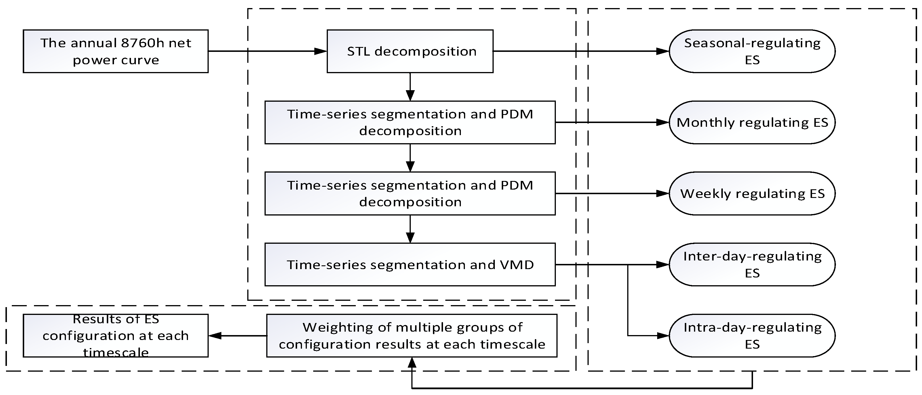
To address the above problems in processing long-period fluctuations and long time series, this paper proposes a HES configuration strategy based on multi-timescale trend decoupling and hierarchical configuration. This strategy draws on the idea of the PDM module in the advanced time-series model time-mixer and solves the difficult problem of ES decoupling and matching under multi-scale fluctuations by gradually stripping trend components at different timescales. The detailed steps are as follows.

Step 1: For the annual 8760 h time-series net power curve $P_{\mathrm{year}}$, the STL method is adopted with a trend smoothing window of 2160 h. The quarterly variation trend $P_{\mathrm{year}-\mathrm{T}}$ of the annual net power curve is extracted and used as the basis for the capacity sizing of seasonal regulation ES.

Step 2: After removing the trend $P_{\mathrm{year}-\mathrm{T}}$ smoothed by seasonal regulation ES from the original power curve $P_{\mathrm{year}}$, the remaining seasonal components $P_{\mathrm{year}-\mathrm{S}}$ still contain fluctuations at monthly, weekly, and other timescales. The time series of the remaining seasonal components is divided into four quarters. The PDM module is then adopted to decompose and mix the segmented curves, so as to obtain the trend components $P_{\mathrm{season}-\mathrm{T}}^i,i\in \left[1,4\right]$ containing only monthly fluctuations for each quarter, which serve as the basis for the corresponding ES configuration.

Step 3: For the seasonal components $P_{\mathrm{season}-\mathrm{S}}^i$ of the quarterly time-series net power curve, the time-series segmentation and PDM operation in Step 2 are repeated to obtain the trend components $P_{\mathrm{month}-\mathrm{T}}^j,j\in \left[1,12\right]$ of the monthly time-series net power curve, which are used for the configuration of weekly regulation ES.

Step 4: The seasonal components $P_{\mathrm{month}-\mathrm{S}}^j$ of the monthly time-series net power curve are segmented to obtain the weekly time-series net power curve $P_{\mathrm{week}}^k,k\in \left[1,52\right]$, which is decomposed into multiple modes by the VMD method. The modes with different frequencies correspond to ES at daily and intra-day timescales.

Step 5: Starting from the quarterly timescale, the number of ES configuration results derived at each timescale increases stepwise. Taking monthly regulation ES as an example, although inter-quarterly fluctuations have been eliminated in the previous stage, the 12 sets of power and capacity ratings configured according to the monthly net power trends still differ from one another. To minimize over-configuration and under-configuration of ES, weights are calculated based on the count of values falling into each equally divided numerical interval, yielding a comprehensive benchmark for ES power and capacity.

The schematic flow diagram is shown in Figure 1.

2.2. STL Decomposition of Time Series

The variation trend of the annual 8760 h net power curve is jointly affected by various factors, including uncertain natural factors such as weather, regular production activities, and changes in installed capacity, resulting in considerable volatility. The original sequence with mixed multi-timescale characteristics complicates the power and capacity configuration of ES. Based on the idea of time-series feature decomposition, the STL algorithm is first adopted to decompose the net power sequence into independent periodic components, seasonal components, and residuals, as shown in Equation (1).

$$y_t=S_t+T_t+R_t$$

(1)

where $S_t$, $T_t$, and $R_t$ represent the periodic component, trend component, and residual component at time t, respectively, and $y_t$ is the original sequence.

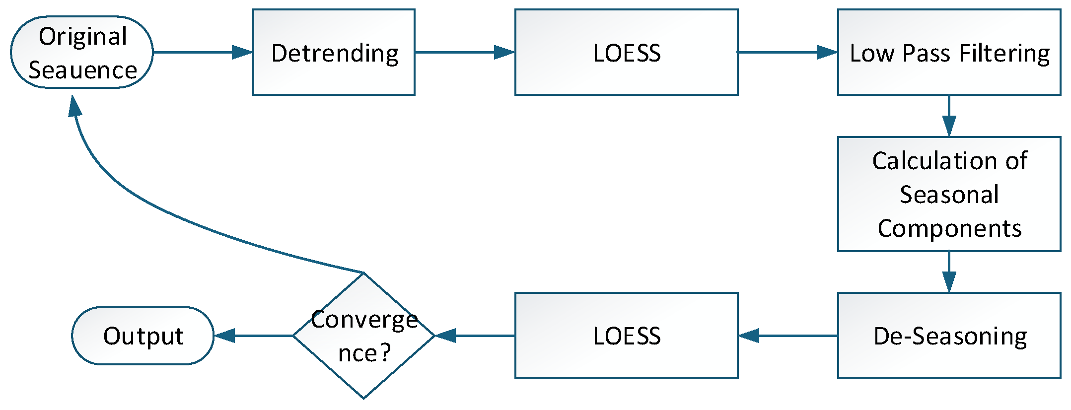
The algorithm is based on a double-layer structure of inner and outer loops. The inner loop performs Locally Estimated Scatterplot Smoothing (LOESS) smoothing on the detrended sequence to derive periodic and trend components, while the outer loop adjusts the robust weights of the algorithm to mitigate the impact of outliers. The algorithm flow is illustrated in Figure 2.

In the outer loop of STL decomposition, robust weights are calculated based on residual terms to update the parameters of LOESS regression in the inner loop. This separates noise points in the data into the residual terms, thereby enhancing the algorithm’s robustness. The robust weights ${\rho }_t$ are calculated using the Bisquare function, which is specifically expressed as:

$$\begin{array}{l}{\rho }_t=B\left(\mu \right)\left\{\begin{array}{l}{\left(1-{\mu }^2\right)}^2,0\le \mu <1\\ 0,\mu \ge 1\end{array}\right.\\ \mu ={\displaystyle \frac{\left|R_t\right|}{6\mathrm{median}\left(\left|R_t\right|\right)}}\end{array}$$

(2)

where $B(\mu )$ denotes the Bisquare function; $R(t)$ represents the residual component; and $\mathrm{median}(.)$ is the median calculation function.

3. New-Type Power System Net Power Decomposition

3.1. Day-Ahead Timescale Power Decomposition Based on PDM Module

The time-mixer model is a time-series forecasting model based on multi-scale fusion architecture. It decouples and mixes multi-scale time series through the PDM module, thereby accurately capturing multi-timescale characteristics [17]. For the residuals obtained after extracting the annual trend from input data via STL, time-series segmentation and the PDM module are adopted to progressively separate fluctuation trends at different timescales, so as to calculate the sizing of ES power and capacity.

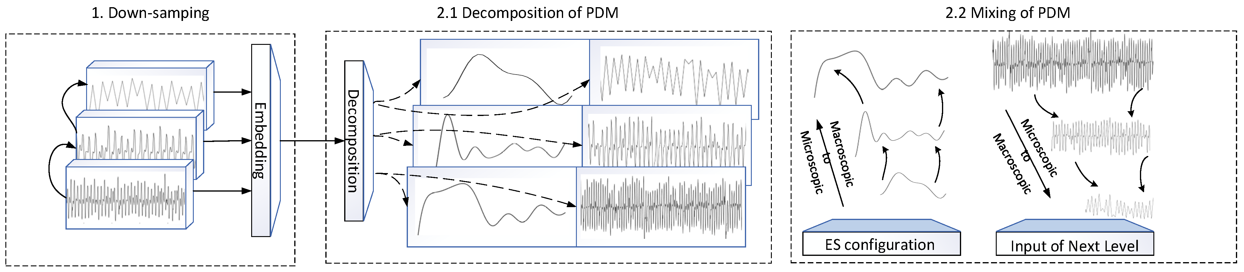
The PDM module samples the original sequence at different time steps, reduces its dimensionality into multiple time series, and decomposes each into trend and seasonal components. The original sequence contains fine variations, while the highest down-sampling dimension captures macroscopic features. By transferring and mixing features across dimensions, final trend and seasonal components are obtained: the trend component is used for ES configuration, and the seasonal component is passed to the next timescale as input for its PDM. The PDM module’s decomposition and reconstruction avoid feature loss from single-timescale trend extraction. Its schematic diagram is shown in Figure 3.

In the $lth$ PDM module, the decomposition block first decomposes the input sequence $X^l$ into a trend component $T^l=\{t_0^l,\dots ,t_M^l\}$ and a periodic component $S^l=\{s_0^l,\dots ,s_M^l\}$. Then, it performs feature mixing on the seasonal components and trend components to realize the multi-scale interaction of the same feature, which is expressed as:

$$\left\{s_m^l,t_m^l\right\}=\mathrm{Decomp}\left(x_m^l\right),l\in \left\{1,\dots ,L\right\},x_m^l\in R^{\left|s_m^l,t_m^l\right|\times d}$$

(3)

$$X^l=X^{l-1}+\mathrm{FeedForward}\left({\mathrm{Mix}}_{\mathrm{S}}\left({\left\{s_m^l\right\}}_{m=0}^{m=M}\right)\right)={\mathrm{Mix}}_{\mathrm{T}}\left({\left\{t_m^l\right\}}_{m=M}^{m=0}\right)$$

(4)

where L denotes the total number of layers; $s_m^l,t_m^l$ are the periodic and trend information with scale m in the $kth$ PDM module; $\mathrm{Decomp}(.)$ is the decomposition block network; $x_m^l$ represents the depth features under different timescales with d channels; $\mathrm{FeedForward}(.)$ is the feedforward layer network composed of two linear layers; and ${\mathrm{Mix}}_{\mathrm{S}}(.)$ and ${\mathrm{Mix}}_{\mathrm{T}}(.)$ are the mixing operation networks for periodic and trend information, respectively.

The decomposition block network obtains the trend component through sliding average processing, takes the remaining part as the periodic component, and ensures the sequence length remains unchanged through Padding operation, where the feedforward network conducts information interaction between channels via the GELU activation function; by virtue of Equation (4), each dimension in the PDM module can extract timescale feature information from the output of the previous dimension, which can gradually capture the complex patterns and top-level features in the original time series and enhance the expressive ability of the module’s output.

In the PDM module, the mixing methods of the seasonal component and the trend component are opposite. In the configuration of ES power and capacity, this paper only considers the top-down mixing direction of the trend component. The seasonal component passed to the next timescale is obtained by subtracting the trend component from the original time series.

In terms of the trend component, subtle and rapid changes in the original data will introduce noise into the macroscopic trend information. However, the trend component of the dimension with the highest down-sampling level can more clearly reflect the slow changes in the original sequence. Therefore, the information of the trend component is transmitted in a top-down direction, so as to guide the fine-scale changes with the overall trend. The trend component $T^l=\{t_0^l,\dots ,t_M^l\}$ is expressed as:

$$T_m^l={\mathrm{Mix}}_{\mathrm{T}}^{\mathrm{Top}-\mathrm{Down}}\left(t_{m-1}^l\right)+t_{m-1}^l$$

(5)

where the periodic term mixing network ${\mathrm{MIX}}_{\mathrm{T}}^{\mathrm{Top}-\mathrm{Down}}(.)$ comprising two linear layers has input and output dimensions of $P/2^{m+1}$ and $P/2^m$, respectively, and its technical architecture also adopts residual connections.

After the initial net power curve passes through multiple PDM modules, net power curves $T^L=\{t_0^L,\dots ,t_M^L\}$ with different timescales and different time-series lengths are obtained. These net power curves at different scales can serve as the basis for ES configuration at corresponding scales.

3.2. Intra-Day Timescale Power Decomposition Based on VMD

For the net power fluctuation components obtained by stripping the trend components at all levels from the original net power curve, this section adopts the VMD algorithm to perform multi-scale decoupling on them.

VMD is a non-recursive signal processing method based on variational theory, which can decompose non-stationary complex signals into K Intrinsic Mode Functions (IMFs) with specific center frequencies. Its core idea is to transform the signal decomposition problem into a constrained variational optimization problem and iteratively find the center frequencies and bandwidths of each mode, thereby achieving effective separation of signals in the frequency domain. Compared with traditional modal decomposition methods, the advantage of VMD lies in the ability to set the value of K independently; however, an excessively large K value will lead to over-decomposition of the original signal, while an excessively small K value will cause mode mixing. To address the problem of presetting the K value, this paper adopts a fixed-value strategy based on spectral analysis, uses FFT to analyze the frequency domain characteristics of the original signal, and presets the K value according to the number of peaks in the frequency spectrum, thus realizing fine-grained extraction of diurnal and intra-day fluctuation characteristics at multiple timescales. The steps are as follows.

Step 1: First, the original signal is sampled at equal intervals to obtain a series of discrete time-domain sequences. The discrete time-domain signal can be expressed as:

$$X\left(n\right)=X\left({\displaystyle \frac{n}{F_s}}\right),n=0,1,2,\dots ,N-1$$

(6)

where $F_s$ is the sampling frequency, N is the total number of sampling points, $X(n)$ is the signal amplitude of the nth sampling point, and $X(t)$ is the original signal.

Step 2: We perform FFT on the discrete time-domain signal to obtain the frequency domain sequence, and conduct amplitude normalization correction:

$$\begin{array}{c}X\left(k\right)={\displaystyle \sum _{n=0}^{N-1}x\left(n\right)e^{-j\frac{2\pi }{N}kn}},k=0,1,2,\dots ,N-1\\ A\left(k\right)={\displaystyle \frac{\left|X\left(0\right)\right|}{N}},k=0\\ A\left(k\right)={\displaystyle \frac{2\left|X\left(k\right)\right|}{N}},k=1,2,\dots ,\left(N/2\right)-1\\ A\left(N/2\right)={\displaystyle \frac{\left|X\left(N/2\right)\right|}{N}},k=N/2\end{array}$$

(7)

where k is the frequency domain index.

Step 3: We use the single-sided spectrum to map the actual frequency corresponding to the frequency domain index k, and determine the value of K based on the number of peaks in the frequency spectrum:

$$f\left(k\right)={\displaystyle \frac{k}{N}}{F}_s$$

(8)

Step 4: After determining the value of K, VMD is performed on the original signal, and its constrained variational model is as follows:

$$\left\{\begin{array}{l}{\min }_{\left\{u_k\right\},\left\{{\omega }_k\right\}}{\displaystyle {\sum }_{k=1}^K{‖{\partial }_t\left[\left(\delta \left(t\right)+\frac{j}{\pi t}\right)\ast u_k\left(t\right)\right]e^{-j{\omega }_{k}t}‖}_2^2}\\ \mathrm{s}.\mathrm{t}.\begin{array}{c}{\displaystyle {\sum }_{k=1}^K{u}_k\left(t\right)}=X\left(t\right)\end{array}\end{array}\right.$$

(9)

where $\left\{u_k\right\}$ is the set of IMFs to be solved; $\hspace{0.17em}\left\{{\omega }_k\right\}$ are the center frequencies corresponding to each IMF; ${\partial }_t$ is the partial derivative in the time domain; and $\delta (t)$ is the Dirac function.

Step 5: We introduce the penalty factor $\alpha$ and Lagrange multiplier $\lambda (t)$ to convert the constrained variational problem into an unconstrained one:

$$L\left(\left\{u_k\right\},\left\{{\omega }_k\right\},\left\{\lambda \right\}\right)=\alpha {\displaystyle {\sum }_{k=1}^K{‖{\partial }_t\left[\left(\delta \left(t\right)+\frac{j}{\pi t}\right)\ast u_k\left(t\right)\right]e^{-j{\omega }_{k}t}‖}_2^2}+{‖X\left(t\right)-{\displaystyle {\sum }_{k=1}^K{u}_k\left(t\right)}‖}_2^2+〈\lambda \left(t\right),X\left(t\right)-{\displaystyle {\sum }_{k=1}^K{u}_k\left(t\right)}〉$$

(10)

Step 6: We adopt the alternating direction multiplier method to iteratively solve Equation (10), and the iterative formula is as follows:

$$\begin{array}{l}{\widehat{u}}_k^{n+1}\omega ={\displaystyle \frac{\widehat{X}\left(\omega \right)-{\displaystyle {\sum }_{i\ne k}{u}_i^{n+1}\left(\omega \right)}+\frac{{\widehat{\lambda }}^n\left(\omega \right)}{2}}{1+2\alpha \left(\omega -{\omega }_k^n\right)}}\\ \hspace{1em}{\omega }_k^{n+1}={\displaystyle \frac{{\displaystyle {\int }_0^{\infty }\omega {\left|{\widehat{u}}_k^{n+1}\left(\omega \right)\right|}^{2}d\omega }}{{\displaystyle {\int }_0^{\infty }{\left|{\widehat{u}}_k^{n+1}\left(\omega \right)\right|}^{2}d\omega }}}\\ {\widehat{\lambda }}^{n+1}\left(\omega \right)={\widehat{\lambda }}^n\left(\omega \right)+\tau \left(\widehat{X}\left(\omega \right)-{\widehat{u}}_k^{n+1}\left(\omega \right)\right)\end{array}$$

(11)

Step 7: We determine whether the precision error ${\displaystyle {\sum }_{k=1}^K{‖u_k^{n+1}-u_k^n‖}_2^2/{‖u_k^n‖}_2^2}$ is satisfied; if satisfied, the iteration ends, and K modal components sorted from high to low frequency are obtained as shown in the following formula, otherwise, we return to Step 4 to continue the iteration.

$$P_t^{\mathrm{Imb}}-L_t^{\mathrm{Imb}}={\displaystyle {\sum }_{k=1}^K{u}_{k,t}}$$

(12)

4. Results

4.1. Background

This case study is set against the practice of carbon-neutral transition in a region in Eastern China, where a power system analysis scenario is constructed. This region features unique ecological positioning and abundant resource endowments and has actively promoted the transformation of its energy structure in recent years. With high-penetration RE integration as the core objective, it is committed to building a demonstration project of a carbon-neutral transition. Its power system exhibits the following typical characteristics:

• This region boasts abundant wind and solar energy resources, with a high share of installed wind and solar capacity that has become the mainstay of its electricity supply. Driven by seasonal and meteorological factors, wind and solar power generation show pronounced intra-day, monthly, and quarterly fluctuations, leading to a clear spatio-temporal mismatch between their output profiles and load demand.
• No conventional thermal power or other dispatchable power sources are deployed in the region, and neither generation expansion planning nor grid planning has been implemented in the context of a carbon-neutral transition. System flexibility therefore relies predominantly on ES, giving rise to an urgent demand for the regulation capability of long-duration ES.

In this paper, the annual actual wind–solar output data and load data of the region are adopted. The annual net power curve, obtained by subtracting load demand from wind–solar output, is used as the input data for the strategy model. When the power value of the net power curve is positive, it indicates that wind–solar generation exceeds load demand at that moment, and the surplus power needs to be shifted to other periods via ES. When the value is negative, it indicates that wind–solar generation is insufficient to meet load demand, and energy needs to be supplied from other periods through ES.

The wind–solar net output is decomposed at multiple timescales by the STL-PDM-VMD strategy model, yielding a series of trend curves and modes corresponding to energy shifting at different timescales, on the basis of which the sizing of ES power and capacity is calculated. In the initial stage of ES configuration planning for the carbon-neutral transition, it is difficult to solve the problem with optimization models due to the lack of relevant economic parameters. Meanwhile, to prevent over-sizing of ES under the influence of extreme factors, statistical distributions are employed in this case study to determine the power and capacity of the ES.

4.2. Multi-Timescale Decomposition Results of Net Power for the Carbon-Neutral Transition

We assume that the discretized power curve ${\tilde{P}}_n$ is partitioned into M half-wave intervals $I_j=\left[a_j,b_j\right]$ via zero-crossing detection. The characteristic quantity of the $jth$ half-wave segment is defined as:

$$\begin{array}{l}{P}_j=\underset{n\in I_j}{\max }\left|{\tilde{P}}_n\right|\\ T_j=\left(b_j-a_j+1\right)\Delta t\\ E_j=P_j\cdot T_j\cdot \lambda \end{array}$$

(13)

Sample sets are constructed respectively as follows:

$${\rm P}={\left\{P_j\right\}}_{j=1}^M,\Gamma ={\left\{T_j\right\}}_{j=1}^M,{\rm E}={\left\{E_j\right\}}_{j=1}^M$$

(14)

The statistical feature extraction function is defined as:

$$f\left(\chi \right)=\left\{\begin{array}{l}\mu \chi ,M<M_{\min }\\ \mu \chi +1.96\sigma ,\chi \hspace{1em}\mathrm{is}\hspace{1em}\mathrm{approximately} \mathrm{normal}\\ Q_{0.95}\left(\chi \right),\chi \hspace{1em}\mathrm{is}\hspace{1em}\mathrm{non}-\mathrm{normal}\end{array}\right.$$

(15)

Accordingly, the configured power of ES is given by:

$$P^{\ast }=f\left({\rm P}\right)$$

(16)

The characteristic duration is expressed as:

$$T^{\ast }=f\left(\Gamma \right)$$

(17)

The configured capacity of ES is obtained as:

$$E^{\ast }=P^{\ast }\cdot T^{\ast }\cdot \lambda$$

(18)

where $a_j$ denotes the index of the starting sampling point of the $jth$ half-wave interval; $b_j$ denotes the index of the ending sampling point of the $jth$ half-wave interval; M denotes the total number of valid half-wave intervals, i.e., the number of extracted samples; $\mu$ denotes the sample mean; $\sigma$ denotes the sample standard deviation; and $\lambda$ denotes the waveform shape factor, which serves as a correction coefficient for approximating the half-wave area by the product of the maximum power and the duration, and is set to 0.5.

4.2.1. Seasonal-Regulating ES Configuration

Based on the time-series STL decomposition model in Section 2.2, trend extraction is performed on the annual 8760 h net power curve. The obtained trend curve $P_{\mathrm{year}-\mathrm{T}}$, which serves as the basis for seasonal-regulating ES capacity configuration, is shown in Figure 4. The black curve represents the annual imbalance power obtained by subtracting the load from wind–solar generation, which serves as the input data of the strategy model and corresponds to the left ordinate. The blue dashed curve is the trend curve of the black curve, corresponding to the right ordinate.

The black curve in the figure shows the hourly raw fluctuation of the annual 8760 h wind–solar net output for a carbon-neutral transition region in Eastern China, and the blue dashed line is the annual trend component extracted using the STL time-series decomposition model. In this STL decomposition, a trend window length of 2160 h is used, which effectively filters out intra-seasonal high-frequency random components such as intra-day and intra-week fluctuations, accurately extracts low-frequency trend variations across multi-month timescales, and clearly characterizes the seasonal evolution of wind–solar net output in this region. The seasonal characteristics of the annual trend curve represented by the blue dashed line are analyzed as follows.

Spring (starting from 1200 h): As the region enters spring, the residential heating load in winter gradually diminishes. Meanwhile, wind and solar resources improve gradually with rising air temperature and longer daylight hours, leading to a continuous upward trend in wind–PV net output, marking the main energy surplus period of the whole year.

Summer (starting from 3500 h): As the region enters summer, it experiences the annual peak solar irradiance, resulting in a substantial increase in solar output. However, the residential cooling load surges simultaneously, causing the wind–solar net output to turn from positive to negative and marking the first major energy deficit period of the year.

Autumn (starting from 5600 h): As the region enters autumn, the cooling load gradually declines and the wind–solar net output rebounds. However, limited by the gradual attenuation of wind and solar resources, the net output remains negative, maintaining a continuous energy deficit state.

Winter (starting from 7500 h): As the region enters winter, solar output decreases significantly due to shorter daylight hours and lower temperatures. Meanwhile, the residential heating load rises sharply, pushing the wind–solar net output further down to the annual trough, resulting in a deep energy deficit period.

Overall, the annual trend curve exhibits a typical “double-peak and double-valley” seasonal pattern. The two peaks appear in spring and autumn, mainly driven by low cooling and heating demands during the transitional seasons, coupled with relatively abundant wind and solar resources, forming energy surplus periods. The two valleys occur in summer and winter, primarily caused by prominent peak cooling and heating loads under extreme temperatures, together with the sharp decline of solar resources in winter, resulting in continuous energy deficits.

This trend accurately reflects the seasonal energy consumption habits of region residents and the seasonal resource endowment of wind and solar power generation, which is the core manifestation of the supply–demand imbalance in the carbon-neutral transition.

4.2.2. Monthly Regulating ES Configuration

After removing the component $P_{\mathrm{year}-\mathrm{T}}(t)$ smoothed by seasonal-regulating ES from the original net power sequence $P_{\mathrm{year}}(t)$, the residual periodic component $P_{\mathrm{year}-\mathrm{R}}(t)$ is obtained as follows:

$$P_{\mathrm{year}-\mathrm{R}}(t)=P_{\mathrm{year}}(t)-P_{\mathrm{year}-\mathrm{T}}(t)$$

(19)

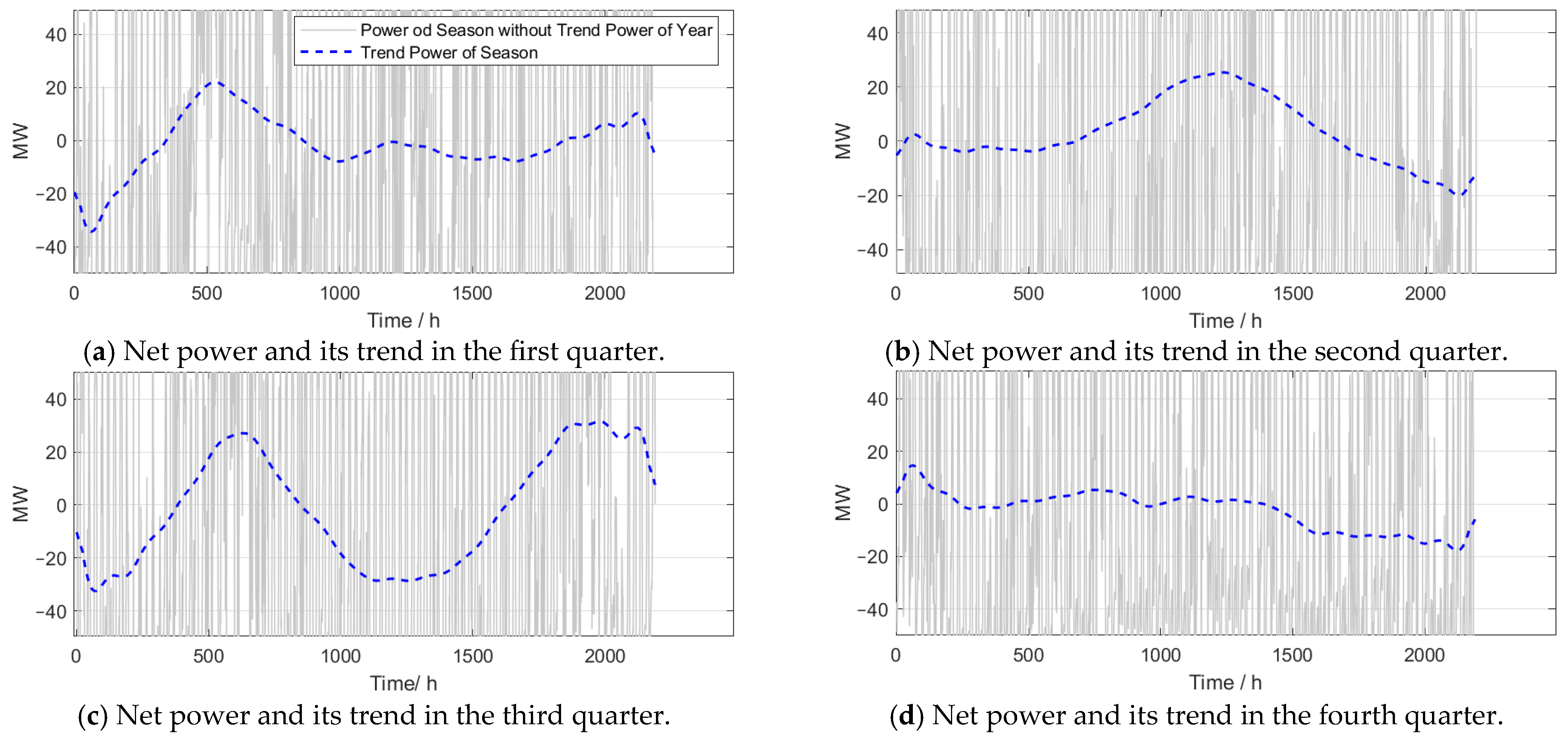
$P_{\mathrm{year}-\mathrm{R}}(t)$ is the annual time-series net power curve. Based on the strategy of ES capacity configuration in Section 2.1, time-series segmentation is carried out to obtain the net power curves of four quarters. The hybrid PDM decomposition procedure in Section 3.1 is applied to each quarterly net power curve, so as to obtain the corresponding trend curves used for configuring the power capacity of monthly regulating ES. The net power curves of the four quarters and their respective trend curves are shown in Figure 5.

The quarterly trend fluctuations extracted by the PDM module for the four quarters are shown in the figure above, reflecting the slow variation process of monthly scale energy imbalance within each quarter. All trend curves fluctuate near the zero line, indicating that the STL module has effectively removed the lower-frequency inter-quarterly fluctuations.

The power of inter-monthly regulation ES is related to the extreme values of the trend curve, approximately 30 MW. Its capacity is associated with the half-wave period of the trend curve, whose average half-wave period is roughly one-third of a quarterly time-series length, indicating that energy should be shifted between inter-monthly time sequences.

4.2.3. Weekly Regulating ES Configuration

When configuring the ES power capacity at timescales shorter than the weekly regulation level, only one group of curves grouped by the upper-level timescale will be used for subsequent analysis due to the excessive number of corresponding curves.

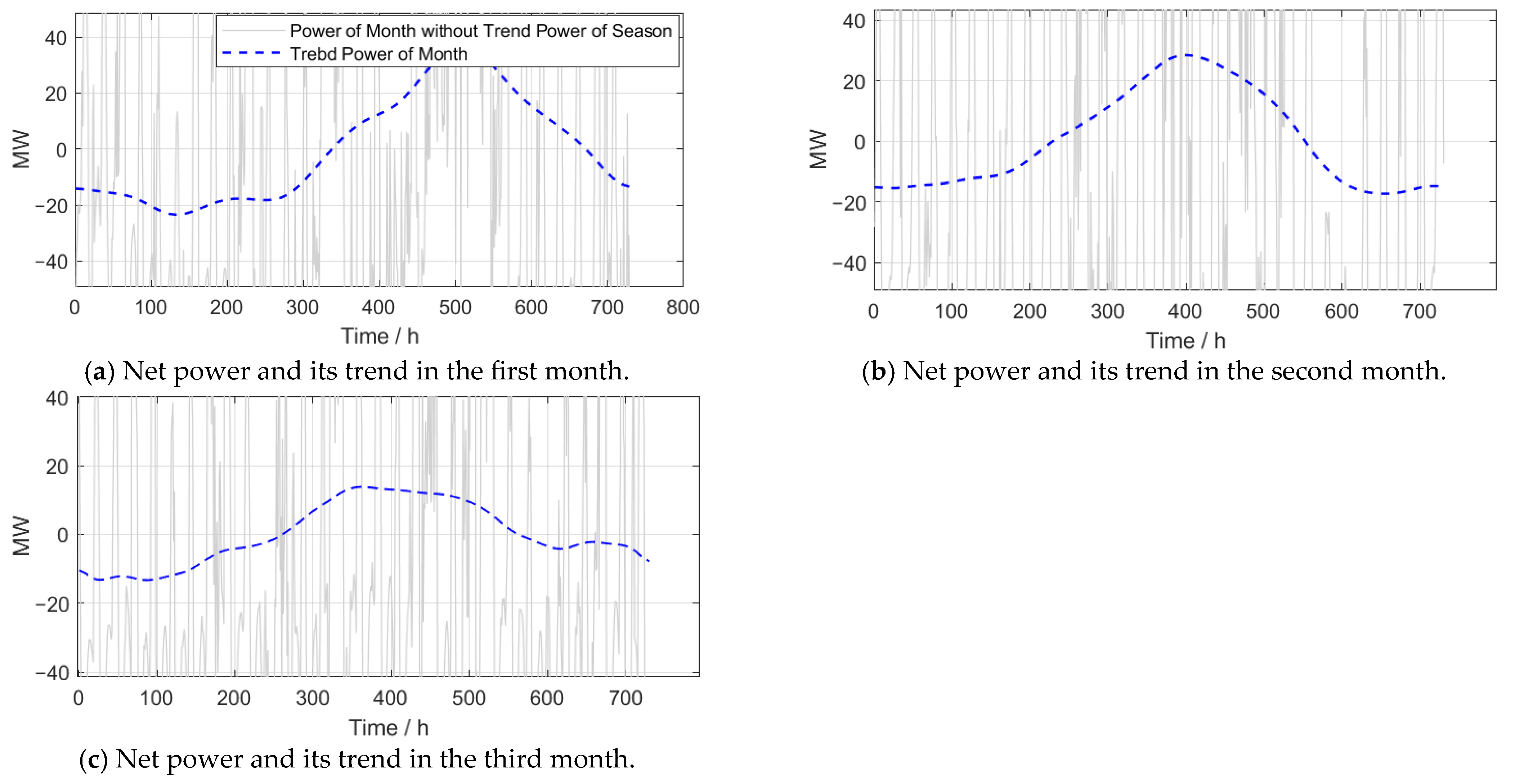
The original power curves and their trends after decoupling the three-month time series from the upper-level scale in the first quarter are shown in Figure 6.

The monthly trend fluctuations extracted by the PDM module for the three months in the first quarter are shown in the figure above, reflecting the slow variation in weekly scale energy imbalance within each month. The trend curves fluctuate near the zero line, indicating that the upper-level PDM module has effectively eliminated the lower-frequency inter-monthly fluctuations.

The power of inter-weekly regulation ES is related to the extreme values of the trend curve, approximately 30 MW. Its capacity is associated with the half-wave period of the trend curve, with an average half-wave period of about half a monthly time-series length. Obviously bi-weekly fluctuations within the month indicate that energy should be shifted between bi-weekly periods.

4.2.4. Inter-Day and Intra-Day Regulation ES Configuration

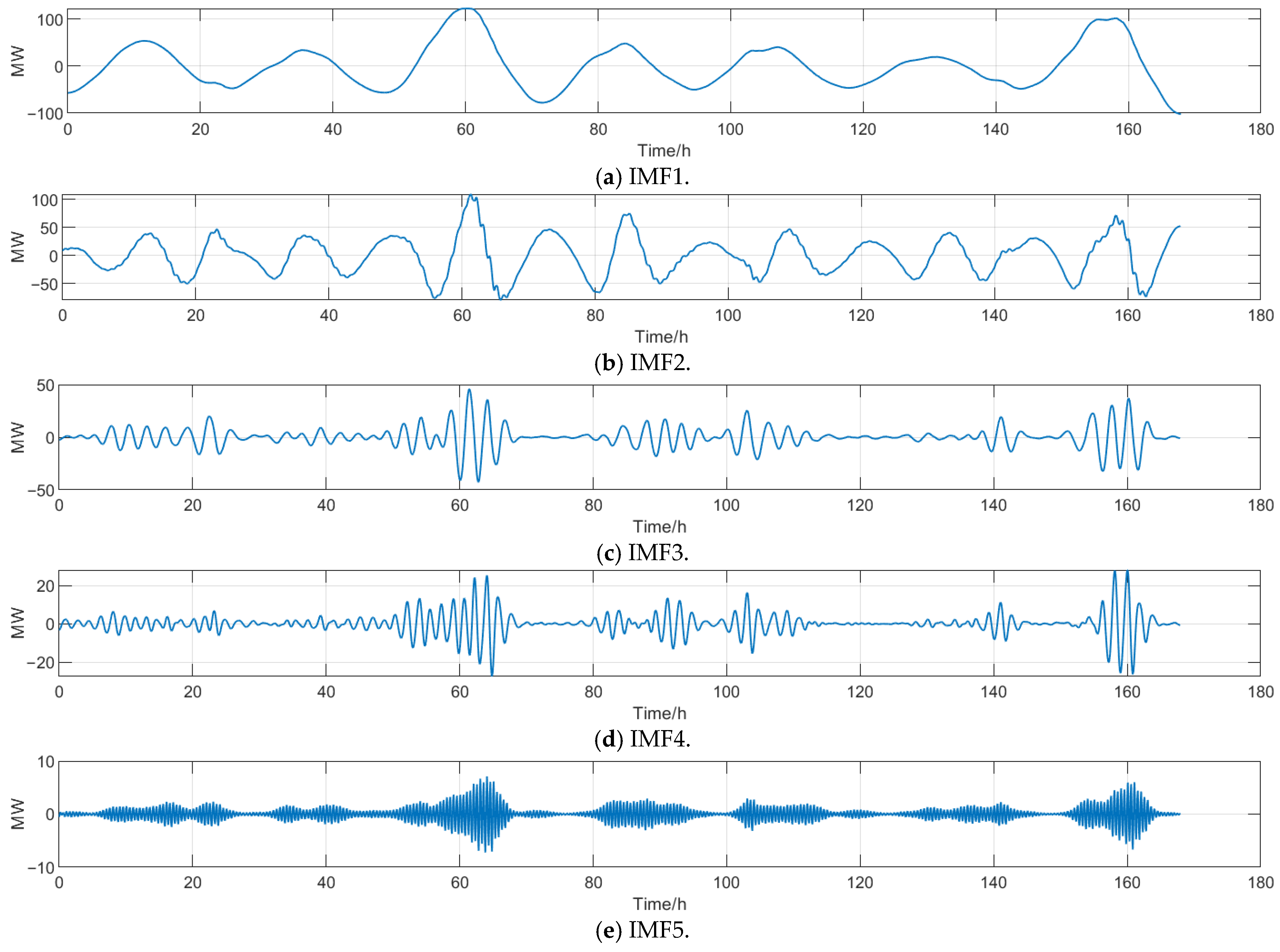
Starting from the configuration of inter-day and intra-day ES at the weekly timescale, the length of the time series to be decomposed and the number of timescales are greatly reduced. Therefore, the VMD algorithm in Section 3.2 is adopted to fully decompose the weekly time-series data, and the corresponding mode components are shown in Figure 7.

According to their respective frequencies, IMF 1 to 5 corresponds to inter-day-regulation 24 h ES, intra-day 12 h ES, intra-day 3 h ES, intra-day 1.5 h ES, and intra-day 0.5 h ES, respectively.

4.2.5. Multi-Timescale Decomposition via the Gurobi–VMD Method

The conventional VMD method is employed to decompose the 8760 h net power curve, and the Gurobi solver is used to obtain optimal decomposition level K. To avoid excessive computational complexity, the intra-hour fluctuations of the raw data are not further expanded, and only the decomposition results at timescales longer than 12 h within a day are compared.

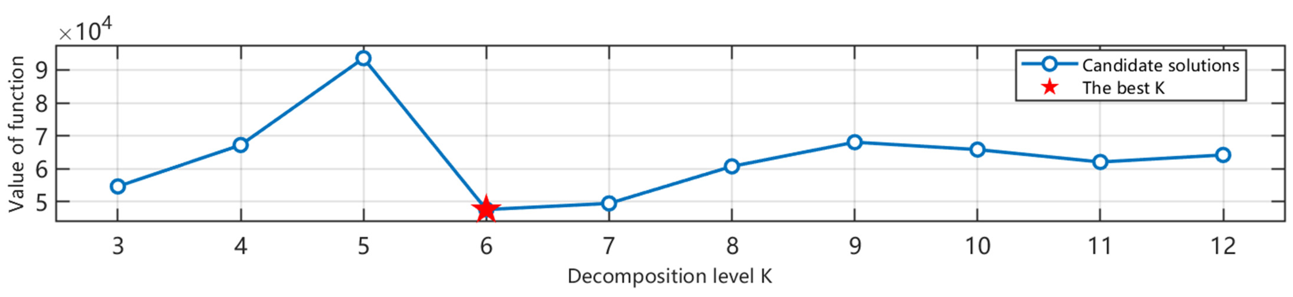
Taking the minimization of power and energy capacity sizing as the objective function, the optimized decomposition level K solved by the solver is shown in Figure 8.

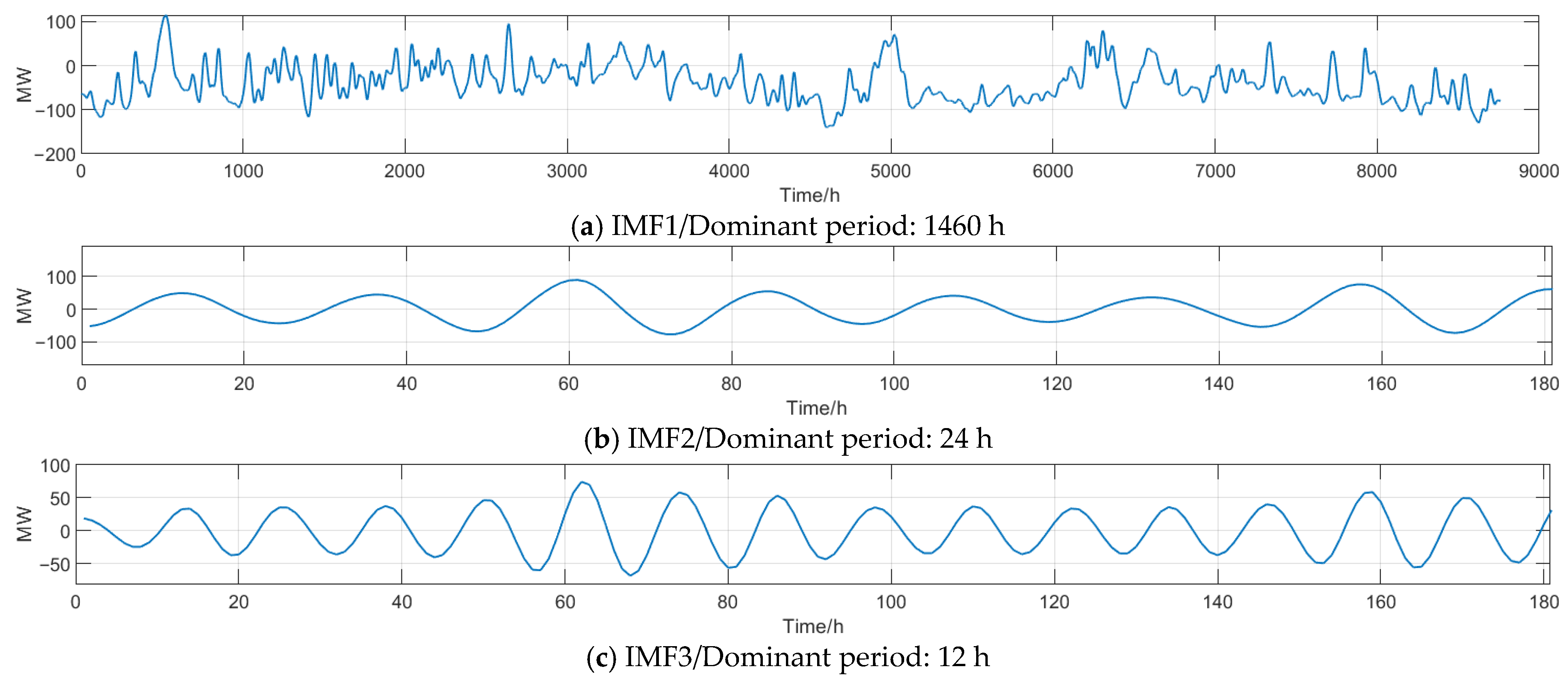
The number of decomposition levels optimized by the solver is close to that obtained by the STL-PDM-VMD method. However, among the IMFs derived from VMD of the input data, IMFs dominated by inter-monthly and inter-weekly fluctuations are missing. Meanwhile, IMF 1 with a dominant period of 1460 h is evidently aliased with fluctuations of finer timescales.

The IMFs corresponding to timescales of 12 h and above in dominant period, decomposed by the Gurobi–VMD method, are presented in Figure 9.

From the decomposition results of Gurobi–VMD, it can be observed that when directly performing VMD on the original 8760 h net power series, obvious low-frequency–high-frequency aliasing still appears in the obtained IMFs, even if the decomposition level K is optimized by the Gurobi. Specifically, low-frequency seasonal IMFs still contain prominent short-period sawtooth fluctuations, while medium-scale IMFs corresponding to inter-monthly and inter-weekly variations are difficult to separate stably.

The proposed STL-PDM-VMD method in this paper first strips out the large-scale trend and then conducts fine-scale decomposition on the local residuals, which is more conducive to obtaining results that match the hierarchical regulation requirements of ES.

4.3. Day-Ahead and Intra-Day Regulation ES Configuration

After performing the above decomposition steps on the annual 8760 h time-series net power curve, the configuration of ES power capacity at each timescale is calculated according to Section 3.2. ES configuration results at each timescale are shown in

Table 1. ES configuration results at each timescale.

Name	Valur of Power	Value of Capacity	Maximum Charge/Discharge Duration
Seasonal-regulating ES	29.7 MW	50,747 MWh	1708.6 h
Monthly regulating ES	35.3 MW	23,988 MWh	679.5 h
Weekly regulating ES	32.2 MW	7592.6 MWh	235.9 h
Inter-day-regulating ES	84.9 MW	1358.4 MWh	16.8 h
Intra-day-regulating ES 1	53.3 MW	341.2 MWh	6.4 h
Intra-day-regulating ES 2	52.6 MW	89.24 MWh	1.7 h
Intra-day-regulating ES 3	33.2 MW	27.6 MWh	0.8 h
Intra-day-regulating ES 4	5.1 MW	1.53 MWh	0.3 h

:

It can be seen from the configuration results in Table 1 that the power values of 24 h and 12 h regulating ES corresponding to diurnal regulation and intra-day regulation 1 are the highest among all timescales, which correspond to the daily solar output peak and the morning and evening load peaks within a day, respectively. Among them, the ES configuration capacity corresponding to seasonal regulation is the highest at all timescales. This is because seasonal-regulating ES requires continuous charging or discharging within a quarter, and even with a low-configured power value, the required capacity far exceeds that at other timescales. The original power balance between generation and consumption in the test system was achieved based on the peak regulation capabilities of hydropower and thermal power units. In the case study of this paper, the output of original hydropower units is replaced by ES, which is configured at multiple timescales. This verifies the effectiveness of the proposed ES configuration strategy for long-period and long-sequence decomposition at the multi-timescale level.

4.4. Input Parameter Sensitivity Analysis

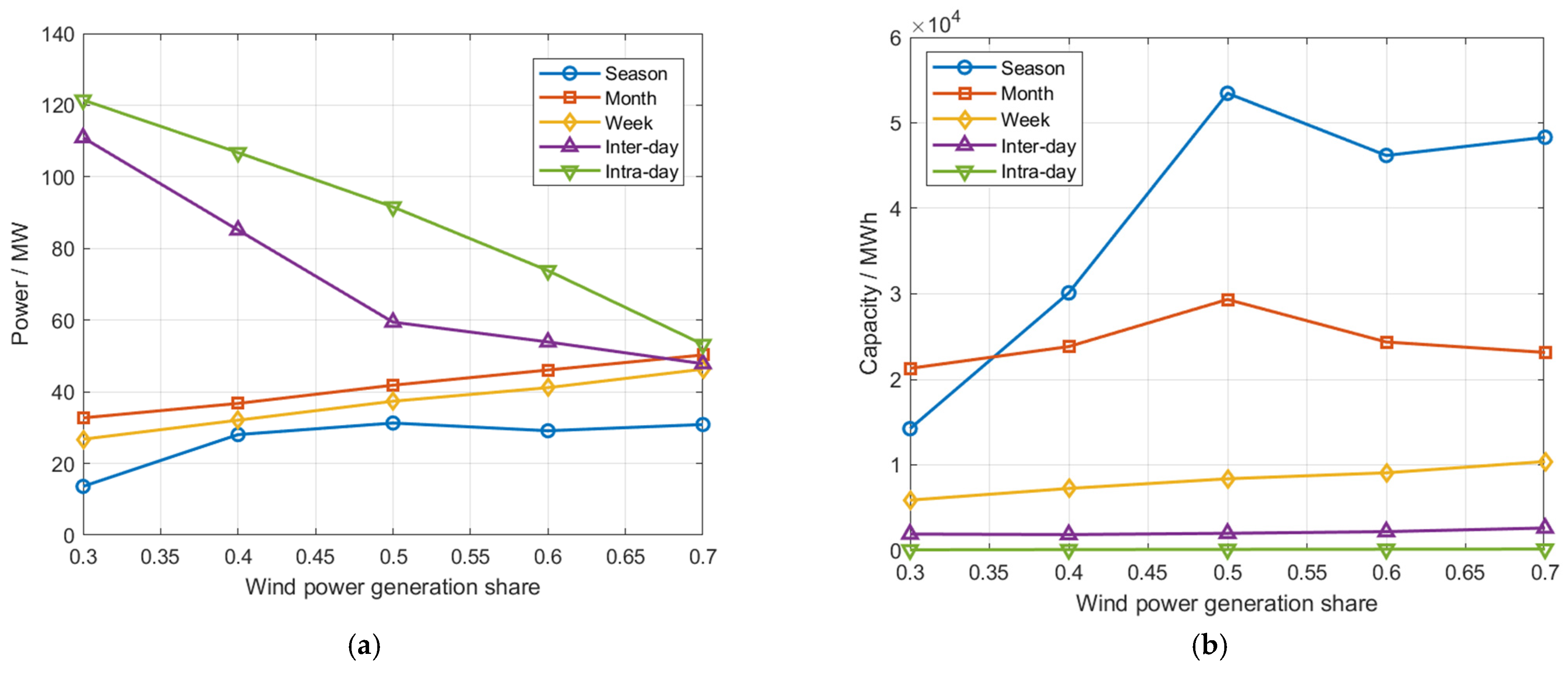
The input data used in the case study are calculated based on the actual wind–solar output and load data of a certain region. By varying the proportion of wind power and solar power in the total wind–solar output, the resulting ES sizing results at different timescales under various wind–solar penetration ratios are shown in Figure 10.

As can be seen from Figure 10a, solar power output exhibits more pronounced diurnal and intra-day fluctuation characteristics. With the gradual increase in the proportion of wind power output, the power capacity of ES for diurnal and intra-day timescales shows a downward trend, whereas the power capacity of ES for inter-weekly, inter-monthly, and seasonal timescales is less affected by variations in the wind–solar output ratio.

As shown in Figure 10b, wind power output features stronger inter-monthly and seasonal fluctuation characteristics. With changes in the wind power ratio, the energy capacity sizing for inter-monthly and seasonal regulation varies significantly. When the wind power ratio rises to 0.5, the energy capacity for inter-monthly and seasonal regulation reaches its maximum. However, since solar power output also presents inter-monthly and seasonal fluctuation characteristics, the energy capacity sizing for inter-monthly and seasonal regulation gradually decreases as the wind power ratio further increases.

5. Conclusions and Future Work

This paper addresses the problem of HES configuration planning in the initial stage of carbon-neutral transition development and proposes a multi-timescale HES configuration framework based on STL-PDM-VMD. Long-period and long-time-series net power curves are decomposed using the proposed framework. The effectiveness of the presented method is verified through case analysis, and the following conclusions are drawn.

The multi-timescale decoupling and hierarchical configuration procedure can explicitly decompose the long-period fluctuations in long sequences and characterize the energy transfer requirements of the power system at various timescales. By employing the PDM module in the time-mixer model to fuse features of different dimensions in a top-down manner, the trend representation capability of the model is strengthened.

The ES power and capacity sizing results obtained from the case study are derived solely by deploying ES for wind–solar accommodation and energy shifting, without considering the reserve capacity support of thermal power units at annual, seasonal, and monthly levels. The results indicate that extremely high sustained charge–discharge capability of ES is required, and the corresponding configured capacity is considerably large.

In future research, constrained hydropower units and reserve capacity of thermal power units can be further incorporated into multi-timescale ES power and capacity sizing. Alternatively, economic parameters of various ES technologies can be considered to establish an optimization model for solving the optimal ES configuration scheme.

References

1. Meng, L.; Zafar, J.; Khadem, S.K.; Collinson, A.; Murchie, K.; Coffele, F. Fast Frequency Response from Energy Storage Systems—A Review of Grid Standards, Projects and Technical Issues. IEEE Trans. Smart Grid 2019, 11, 1566–1581. [Google Scholar] [CrossRef]
2. Xie, X.; Ma, N.; Liu, W.; Zhao, W.; Xu, P.; Li, H. Functions of Energy Storage in Renewable Energy Dominated Power Systems: Review and Prospect. CSEE JPES 2022, 43, 158–168. [Google Scholar] [CrossRef]
3. Zhang, Y.; Xu, Y.; Guo, H.; Zhang, X.; Guo, C.; Chen, H. A hybrid energy storage system with optimized operating strategy for mitigating wind power fluctuations. Renew. Energy 2018, 125, 121–132. [Google Scholar] [CrossRef]
4. Iris, Ç.; Lam, J.S.L. Optimal Energy Management and Operations Planning in Seaports with Smart Grid while Harnessing Renewable Energy under Uncertainty. Omega 2021, 103, 102445. [Google Scholar] [CrossRef]
5. Shi, Z.; Fan, F.; Tai, N.; Qing, C.; Meng, Y.; Guo, R. Coordinated Operation of the Multiple Types of Energy Storage Systems in the Green-Seaport Energy-Logistics Integrated System. IEEE Trans. Ind. Appl. 2024, 60, 4482–4493. [Google Scholar] [CrossRef]
6. Yin, J.; Jiang, Y.; Wei, T. Energy Management Method for Port Areas Microgrid with Hydrogen-Electric Hybrid Energy Storage. Acta Energ. Sol. Sin. 2025, 46, 58–67. [Google Scholar]
7. Zhang, X.; Zhou, S.; Lu, Y.; Huo, F.; Jiao, F.; Zhang, Y. Dual-Layer Fuzzy Mapping-Based Dynamic Power Allocation Strategy for Electric-Hydrogen Hybrid Energy Storage System. IEEE Trans. Ind. Electron. 2025, 72, 10316–10326. [Google Scholar] [CrossRef]
8. Liu, Z.; Qi, G.; Gao, J.; Wang, Z. Research on Optimal Configuration of Hybrid Energy Storage Capacity Based on Adaptive VMD. Acta Energ. Sol. Sin. 2022, 43, 75–81. [Google Scholar] [CrossRef]
9. Zhang, Y.; Jing, S.; Wei, Y.; Huang, Z.; Gao, F. A Power Allocation Strategy for Hybrid Energy Storage System Based on Dynamic Virtual Impedance Network. IEEE Trans. Power Electron. 2025, 40, 17256–17266. [Google Scholar] [CrossRef]
10. Wu, Z.; Zhou, M.; Wang, J.; Yang, W.; Yuan, B.; Li, G. Review on Market Mechanism to Enhance the Flexibility of Power System Under the Dual-carbon Target. CSEE JPES 2022, 42, 7746–7764. [Google Scholar]
11. Ding, Q.; Zhao, B.; Chen, C.; Wan, C.; Zhang, L. Coordinated Configuration Optimization of Hybrid Electric-hydrogen Energy Storage in Microgrids Based on Multi-time Scale Feature Extraction. CSEE JPES 2025, 45, 8867–8879. [Google Scholar] [CrossRef]
12. Lin, Z.; Wang, Z.; Zhang, F.; Wang, R. Research on Optimization Method for Energy Capacity Configuration in Solar DC Micro Grid Considering Hydrogen Energy Application. High Volt. Appar. 2024, 60, 78–87. [Google Scholar] [CrossRef]
13. Feng, J.; Hu, Z.; Duan, X.; Cai, S.; Zhang, P. A Multi Stage DRO-SDDP Approach for Planning Multi-Type Energy Storage Systems and Flexible Resources in High-Penetration Renewable Power Systems. IEEE Trans. Ind. Appl. 2025, 61, 5853–5897. [Google Scholar] [CrossRef]
14. Fang, K.; Zhou, M.; Wu, S.; Zhao, Z.; Zhao, H.; Li, Y. Optimal Planning and Cost-benefit Analysis of Long-duration Energy Storage for Low-carbon Electric Power System. CSEE JPES 2023, 43, 8282–8295. [Google Scholar] [CrossRef]
15. Fu, Y.; Zhou, Y.; Ge, X.; Diao, G.; Fei, F.; Huang, R. Multi-objective Planning of Electricity-hydrogen Hybrid Energy Storage for Source-side Power Fluctuation Mitigation in Offshore Wind Farms Across Multiple Time Scales. Power Syst. Technol. 2025, 49, 3244–3255. [Google Scholar] [CrossRef]
16. Yang, T.; Huang, Y.; He, Z.; Wang, D.; Tang, D.; Xie, C. Optimal Configuration of Siting and Sizing for Grid-forming Battery Energy Storage Station Based on Multi-timescale Regulation. Autom. Electr. Power Syst. 2024, 48, 54–64. [Google Scholar]
17. Wang, S.; Wu, H.; Shi, X.; Hu, T.; Luo, H.; Ma, T.; James, Y.Z.; Zhou, J. TimeMixer: Decomposable Multiscale Mixing for Time Series Forecasting. arXiv 2024, arXiv:2405.14616. [Google Scholar] [CrossRef]
Figure 1. Flowchart of multi-timescale HES configuration.
Energies 19 02074 g001
Figure 2. Flowchart of STL.
Energies 19 02074 g002
Figure 3. Flowchart of the PDM module.
Energies 19 02074 g003
Figure 4. Original net power and its annual trend.
Energies 19 02074 g004
Figure 5. Net Power and trend for four quarters within a year.
Energies 19 02074 g005
Figure 6. Net power and trend for three months within a season.
Energies 19 02074 g006
Figure 7. Results of VMD.
Energies 19 02074 g007
Figure 8. Optimization results of decomposition level K.
Energies 19 02074 g008
Figure 9. IMF1~3 of Gurobi–VMD.
Energies 19 02074 g009
Figure 10. IMF1~3 of Gurobi–VMD. (a) Sensitivity analysis of ES power sizing at various timescales under different wind power ratios.; (b) Sensitivity analysis of ES capacity sizing at various timescales under different wind power ratios.
Energies 19 02074 g010