Research on a Sliding Mode Self-Disturbance-Rejection Control Strategy for Three-Phase Interleaved Buck Converters

Abstract

To address the issues of slow dynamic response and poor disturbance rejection in three-phase interleaved parallel buck converters under disturbance conditions such as voltage or load transients, an improved sliding mode auto-disturbance rejection control (SM-ADRC) strategy is proposed. Firstly, the traditional ADRC algorithm suffers from reduced disturbance observation accuracy in the extended state observer (ESO) due to discontinuous switching of the nonlinear function at segment boundaries. To address this, a novel nonlinear function is designed using an interpolation fitting method. Concurrently, an improved ESO is constructed based on deviation-control principles, utilising the deviation between each state variable and its observed value. Secondly, an enhanced state error feedback law combines an improved exponential approach law with an integral sliding mode surface, thereby enhancing the control system’s robustness. Finally, simulation comparisons of output voltage fluctuations and power response speeds under various operating conditions validate the superiority and feasibility of the proposed SM-ADRC strategy over both the conventional ADRC strategy and PI control strategy.

1. Introduction

With the rapid advancement of modern power electronics, buck-type DC–DC converters serve as pivotal components in power conversion, playing a crucial role in diverse power management and industrial applications. Interleaved parallel technology extends the output power of buck converters while reducing input and output current ripple, enabling their widespread adoption in energy storage systems [1,2,3]. Optimising the control strategy of buck converters enhances output voltage stability, thereby improving the system’s dynamic performance.

However, the stability and control performance of three-phase interleaved parallel buck converters remain challenging due to factors such as power supply fluctuations, load variations, and environmental disturbances [4,5,6]. Presently, numerous advanced nonlinear control methodologies have been applied to the control of interleaved parallel buck converters, such as sliding mode control (SMC) [7], active disturbance rejection control (ADRC) [8], passive control [9], and model predictive control [10]. Among these, traditional ADRC still exhibits certain limitations. To further enhance the control performance and disturbance rejection capability of ADRC, various improvement techniques have been proposed. These can be broadly categorised into two groups. The first group focuses on optimising the nonlinear function of the extended state observer (ESO). For instance, ref. [11] introduces a least-squares parameter identification method to modify the nonlinear function, while refs. [12,13] replace it with an anti-chattering factor to improve control performance. Although these approaches enhance observation accuracy to some extent, the underlying nonlinear functions remain piecewise-defined and are non-differentiable at segment boundaries, which can induce high-frequency oscillations and degrade observation precision. The second group adjusts the gain in the large-error segment of the regulation function [14,15]. However, these modifications do not fundamentally resolve the discontinuous switching issue inherent in the ESO structure, leaving room for further improvement in both observation smoothness and dynamic response.

Among various control algorithms, sliding mode control (SMC) has garnered significant attention for its simplicity, high precision, and strong robustness [16,17,18]. A key research focus has been the improvement of the reaching law, which directly affects both convergence speed and chattering suppression. Existing improvement approaches can be broadly categorised into two types. The first category enhances the reaching law by introducing system state variables into its structure. Early efforts, such as [19,20], incorporate state variables into the constant and exponential terms of traditional reaching laws, achieving limited chattering reduction. Reference [21] further refines this idea by designing a state-variable-based reaching law to reduce steady-state error; however, the high switching frequency of the sign function still induces considerable chattering, compromising the dynamic quality of the reaching motion. The second category focuses on modifying the switching function itself to suppress chattering. Studies such as [22,23,24] adopt system-state-adaptive nonlinear coefficients that approach zero near the sliding surface, effectively mitigating chattering caused by fixed gains. Nevertheless, this approach increases nonlinear computational complexity, leading to slower dynamic response and higher real-time implementation difficulty. Reference [25] replaces the sign function with a saturation function to control chattering and overshoot, but its computational process remains complex and limits practical applicability. In summary, existing improved reaching laws struggle to simultaneously achieve fast convergence, low chattering, and low computational burden—a gap that motivates the design of the modified exponential reaching law in this work.

Table 1. Categorisation and limitations of improved ADRC and improved reaching law studies.

Technical Category	Reference	Core Technique/Method	Problem Addressed	Limitation/Gap Filled by This Work
ADRC Improvements
Optimisation of ESO Nonlinear Function	[11]	Least-squares parameter identification to modify the nonlinear function	Enhances ADRC disturbance rejection capability	The nonlinear function remains piecewise-defined and non-differentiable at segment boundaries, which may induce high-frequency oscillations and limit observation accuracy
	[12,13]	Introduction of an anti-chattering factor to replace the conventional nonlinear function	Reduces chattering and improves control performance	The function remains piecewise and non-differentiable; no structural improvement to the ESO is made
Adjustment of Regulation Function Gain	[14,15]	Gain adjustment in the large-error segment of the regulation function	Enhances disturbance rejection under large-error conditions	Does not resolve the discontinuous switching issue inherent in the ESO; observation smoothness and dynamic response remain to be improved
SMC Improvements
Introduction of State Variables into Reaching Law	[19,20]	Incorporation of system state variables into the constant and exponential terms of the reaching law	Mitigates chattering	Chattering suppression is limited; convergence speed and dynamic response are not significantly improved
	[21]	State-variable-based reaching law design	Reduces steady-state error	The high switching frequency of the sign function still induces considerable chattering, compromising the dynamic quality of the reaching process
Modification of Switching Function	[22,23,24]	Adoption of system-state-adaptive nonlinear coefficients that approach zero near the sliding surface	Suppresses chattering caused by fixed gains	Increased nonlinear computational complexity leads to slower dynamic response and greater difficulty in real-time implementation
	[25]	Replacement of the sign function with a saturation function	Controls chattering and overshoot	The computation process remains complex, limiting practical applicability
This Work		Continuously differentiable nonlinear function (sine-tangent interpolation); Improved ESO structure based on deviation control; Modified exponential reaching law incorporating system state variables	Simultaneously improves ESO observation accuracy, convergence speed, and chattering suppression while maintaining low computational complexity	Provides an integrated SM-ADRC framework that combines an enhanced ESO with an improved reaching law, addressing the gap left by previous studies, which failed to balance observation smoothness, dynamic response, and chattering suppression

summarises the categorisation and limitations of existing ADRC and SMC improvement approaches. However, the aforementioned improvements to ADRC and SMC have been developed largely along separate paths. A composite strategy that synergistically integrates an enhanced ESO with a refined sliding mode reaching law remains underexplored, particularly for three-phase interleaved buck converters operating under complex disturbance conditions. Specifically, two critical gaps persist in the existing literature:

(1)

Regarding ADRC, although various modifications to the nonlinear function and gain parameters have been proposed, the fundamental issue of discontinuous switching in the ESO—caused by the non-differentiability of the nonlinear function at segment boundaries—has not been fully resolved. This limitation impairs observation smoothness and dynamic response.

(2)

Regarding SMC, existing improved reaching laws struggle to simultaneously achieve fast convergence, effective chattering suppression, and low computational complexity. Approaches that introduce state variables offer limited chattering reduction, while those that modify the switching function often incur increased computational burden or slower dynamic response.

To bridge these gaps, this paper proposes an enhanced sliding mode active disturbance rejection control (SM-ADRC) composite strategy. The main contributions are threefold: First, a fundamentally new nonlinear function is designed using interpolation fitting with a combination of sine and tangent functions. Unlike existing piecewise functions, this new function is continuous and differentiable across the entire domain, eliminating the high-frequency oscillations caused by non-differentiable points in traditional ESO. Second, building upon this new nonlinear function, an improved ESO is constructed based on deviation control principles. By incorporating the tracking deviations between state variables and their observations as additional control inputs, this structural enhancement accelerates system convergence and further improves observation accuracy. Third, a modified exponential reaching law is proposed by integrating a tuning function and system state variables into the traditional reaching law. This improved law retains the advantages of conventional approaches while achieving faster convergence and more effective chattering suppression. Finally, by combining the improved ESO with the modified reaching law, the proposed SM-ADRC strategy offers an integrated solution that simultaneously addresses observation accuracy, convergence speed, and chattering suppression. Simulation results validate the superiority of this strategy over conventional ADRC and PI control under various operating conditions.

2. Description of the Three-Phase Interleaved Parallel Buck Converter

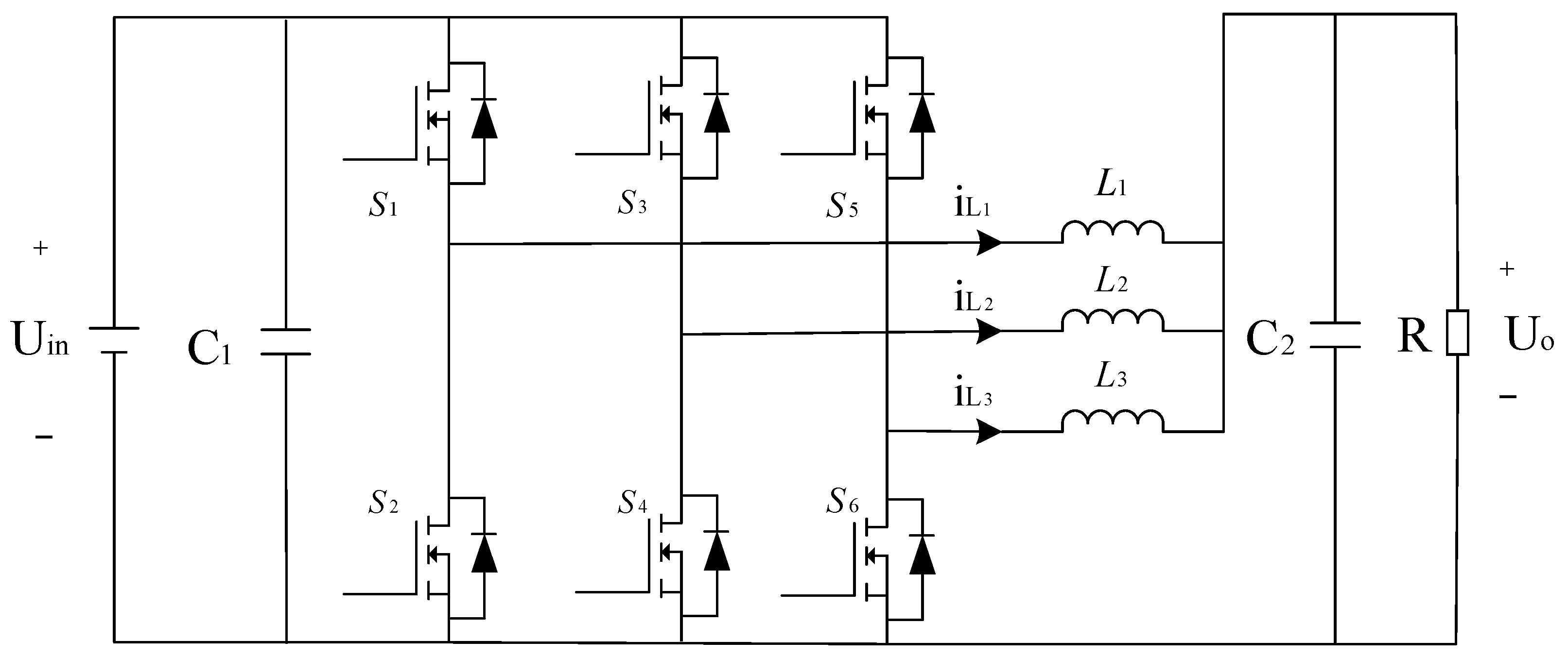
The three-phase interleaved parallel buck converter is illustrated in Figure 1. Its circuit topology employs a multi-phase interleaved parallel configuration, where all switching devices operate at identical frequencies with fixed phase-shifted triggering. Through the superposition of three-phase inductor currents, ripple-generating components partially cancel each other out, significantly reducing output current ripple.

As depicted, the three-phase interleaved parallel buck converter comprises three identical buck converters connected in parallel, where ${\mathrm{U}}_{\mathrm{in}}$ and ${\mathrm{U}}_{\mathrm{o}}$ denote input and output voltages, respectively, C represents the filter capacitor, $S_1~S_6$ are the switching transistors, ${\mathrm{C}}_1$ and ${\mathrm{C}}_2$ denote input and output filter capacitors, respectively, $L_1~L_3$ is the inductor, ${\mathrm{i}}_{\mathrm{L}1},{\mathrm{i}}_{\mathrm{L}2},{\mathrm{i}}_{\mathrm{L}3}$ is the three-phase inductor current, and R is the load. The duty cycles of the switching transistors $S_1, S_3, S_5$ are identical, with trigger phase angles differing by $120°$. This results in a phase shift of $120°$ between the PWM drive waveforms of each phase.

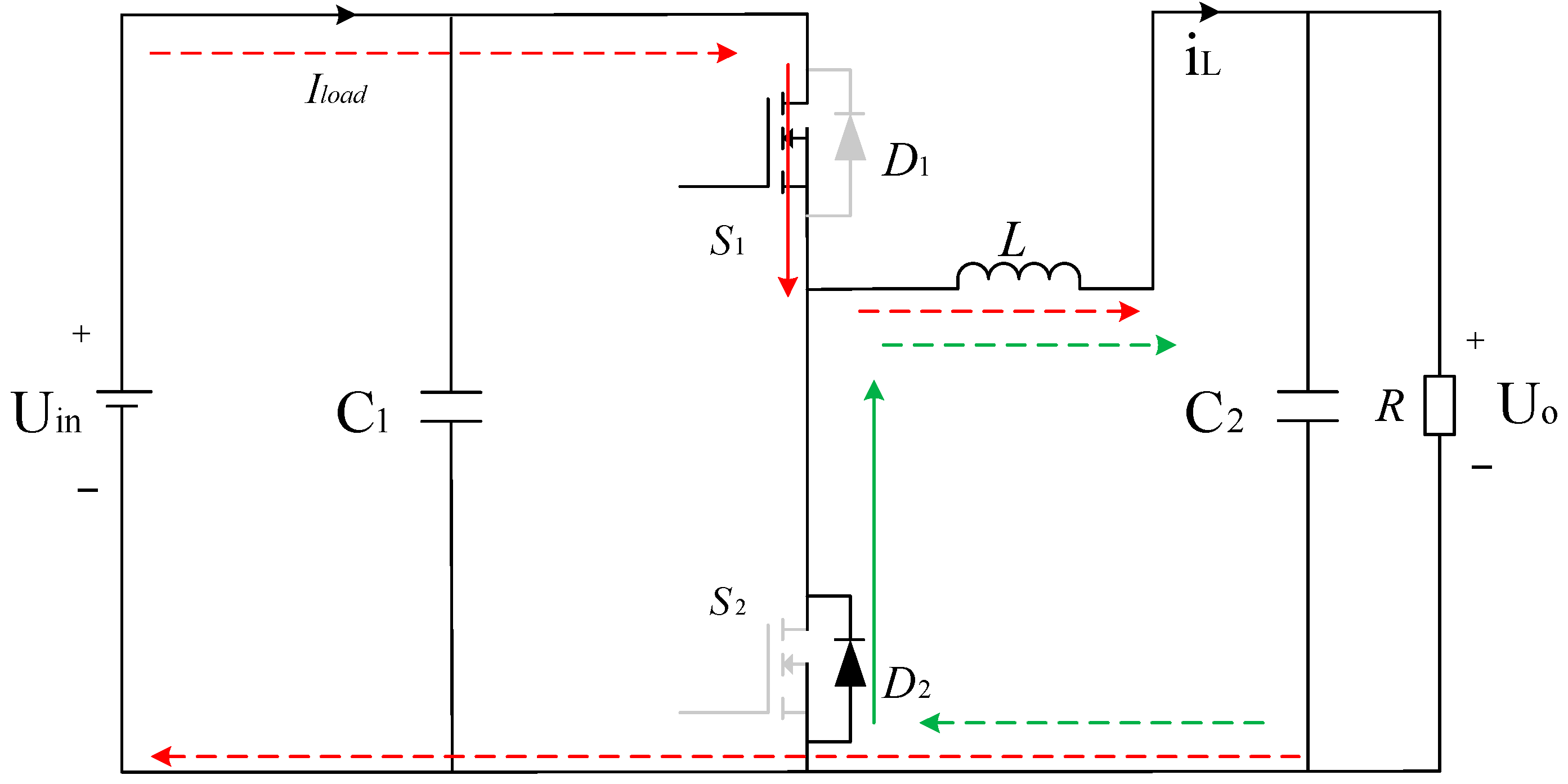
The three-phase interleaved parallel buck converter operates by alternating three converters modules, whose mathematical model can be simplified to that of a single buck converter, as shown in Figure 2. The circuit operates in two states. State 1: Switch $S_1$ is on, $S_2$ is off, and the anti-parallel diode $D_1, D_2$ is off; State 2: Both switches $S_1, S_2$ are off, the anti-parallel diode $D_1$ is off, and $D_2$ is on. Applying Kirchhoff’s laws yields the differential equations for both states:

Neglecting the effects of component parasitic parameters and applying Kirchhoff’s laws, the state–space equations for the symmetrical three-phase interleaved buck converter can be expressed as:

$$\left[\begin{array}{c}{\displaystyle \frac{d{i}_L}{dt}}\\ {\displaystyle \frac{d{U}_o}{dt}}\end{array}\right]=\left[\begin{array}{cc}0& -{\displaystyle \frac{1}{L}}\\ {\displaystyle \frac{1}{C}}& -{\displaystyle \frac{1}{CR}}\end{array}\right]\left[\begin{array}{c}{i}_L\\ U_o\end{array}\right]+\left[\begin{array}{c}{\displaystyle \frac{U_{in}}{L}}\\ 0\end{array}\right]d$$

(1)

where $i_L$ represents the inductor current; L denotes the power inductor; and d is the duty cycle. Applying the Laplace transform yields the transfer function from inductor current to output voltage $G_{vi}\left(s\right)$:

$$G_{vi}\left(s\right)={\displaystyle \frac{U_o\left(s\right)}{i_L\left(s\right)}}={\displaystyle \frac{R}{RCs+1}}$$

(2)

3. Overall Control Strategy Design

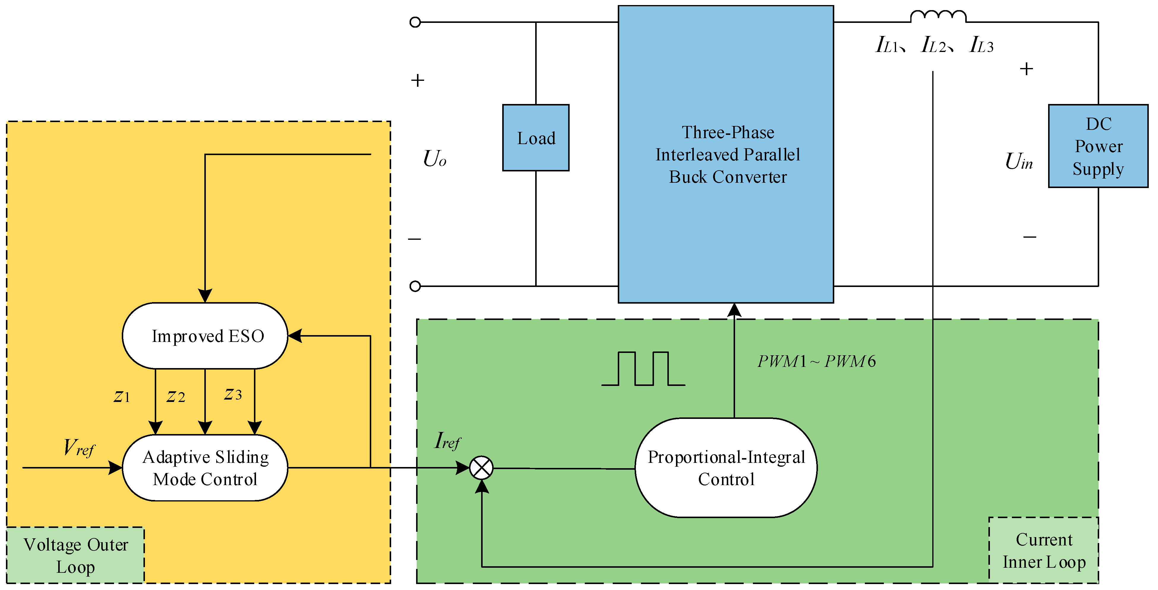
The overall control block diagram is shown in Figure 3. The voltage outer loop incorporates the nal function and deviation control principle to enhance the traditional extended state observer, thereby improving observation accuracy and enabling monitoring of both output voltage and disturbances. Sliding mode control is applied to the state error feedback law, replacing the conventional proportional control component to enhance output voltage tracking speed and compensation. In Figure 3, $Z_1$ represents the observed value of the converter’s output voltage, while $Z_3$ denotes the observed value of the converter’s total disturbance. These observed values are then employed as reference inputs for the current inner loop. The current inner loop adopts a PI current-sharing phase-shift control method to independently regulate the three-phase inductor currents. Finally, a PWM waveform is generated to control the switching of the converter’s power transistors.

3.1. Voltage Outer-Loop Control Strategy Design

3.1.1. Improved Extended State Observer

The controller design is derived from the mathematical model expression in Equation (1). To meet the requirements of self-disturbance-rejection control, the input-to-output expression is rewritten as:

$$y=-ay+b_0{I}_{in}+w=b_{0}u+f(y,I_{in},w)$$

(3)

where $a$ denotes the output variable coefficient; $I_{in}$ represents the inner-loop current reference; $y$ signifies the converter output voltage; $w$ denotes external disturbances, encompassing parameter variations, sampling errors, and unmodelled dynamics; $f_d\left(t\right)$ constitutes the converter’s overall disturbance function; and $b_0$ indicates disturbance compensation, with $b_0=1/G$ and $u=I_{in}$.

Let the state variables be defined as: $x_1=y$, $x_2={\dot{x}}_1=\dot{y}$, $x_3=f_d\left(t\right)$. Then the system’s state equations are:

$$\left\{\begin{array}{l}{\dot{x}}_1=x_2\hfill \\ {\dot{x}}_2=x_3+b_{0}u\hfill \\ {\dot{x}}_3={\dot{f}}_d\left(t\right)\hfill \\ y=x_1\hfill \end{array}\right.$$

(4)

The design equations for the traditional ESO are thus derived as:

$$\left\{\begin{array}{l}e=z_1-y\hfill \\ {\dot{z}}_1=z_2-l_{1}e\hfill \\ z_2=z_3-l_2\mathrm{fal}(e,{\alpha }_1,\delta )+b_{0}u\hfill \\ {\dot{z}}_3=-l_3\mathrm{fal}(e,{\alpha }_2,\delta )\hfill \end{array}\right.$$

(5)

The nonlinear function $fal(e,a,\delta )$ employed in the traditional ESO is piecewise defined at the horizontal coordinates 0 and $\pm \delta$, exhibiting continuity at these junctures. At $x>0$, taking the first derivative of $fal(e,a,\delta )$ yields Equation (6):

$${\displaystyle \frac{d}{dx}}\mathrm{fal}(e,a,\delta )=\left\{\begin{array}{ll}a{x}^{a-1},\hfill & e>\delta \hfill \\ {\displaystyle \frac{1}{{\delta }^{1-a}}},\hfill & 0<e\le \delta \hfill \end{array}\right.$$

(6)

Substituting $e=\delta$ into the above yields:

$$a{\delta }^{a-1}\ne {\displaystyle \frac{1}{{\delta }^{1-a}}}$$

(7)

Equation (7) indicates that $fal(e,a,\delta )$ is not differentiable at $e=\delta$, and similarly not differentiable at $e=-\delta$. This will cause the system to generate high-frequency oscillations, adversely affecting control performance and reducing the observation accuracy of the ESO module.

To resolve these issues, an interpolation-based approach is employed to design an improved nonlinear function $nal(e,a,\delta ,k)$ as follows:

$$nal(e,a,\delta ,k)=\left\{\begin{array}{ll}{\eta }_1\sin (e)+{\eta }_2{\sin }^2(e)+{\eta }_3\tan (e),\hfill & |e|\le \delta \hfill \\ \mathrm{sign}(e)|e{|}^{\alpha },\hfill & \delta <|e|<k\hfill \\ \mathrm{sign}(e)|k{|}^{\alpha },\hfill & k\le |e|\hfill \end{array}\right.$$

(8)

$nal(e,a,\delta ,k)$ Formed by the linear combination of $\sin (e)$, ${\sin }^2(e)$, and $\tan (e)$, the combined use of sine and tangent functions renders $nal(e,a,\delta ,k)$ smoother within the interval and exhibits stronger convergence. To ensure the function is continuous and differentiable at $e=\delta$, the following condition must be satisfied:

$$\left\{\begin{array}{ll}nal(e,a,\delta ,k)={\delta }^a,\hfill & x=\delta \hfill \\ nal(e,a,\delta ,k)=-{\delta }^a\hfill & x=-\delta \hfill \\ na{l}^{\prime }(e,a,\delta ,k)=a{\delta }^{a-1}\hfill & x=\delta \hfill \\ -na{l}^{\prime }(e,a,\delta ,k)=a{\delta }^{a-1}\hfill & x=-\delta \hfill \end{array}\right.$$

(9)

Solving yields:

$$\left\{\begin{array}{l}{\eta }_1={\displaystyle \frac{{\delta }^a-a{\delta }^{a-1}{\cos }^2\delta \tan \delta }{{\sin }^3\delta }}\hfill \\ {\eta }_2=0\hfill \\ {\eta }_3=-{\displaystyle \frac{{\delta }^a\cos \delta -a{\delta }^{a-1}\sin \delta }{\sin \delta {\tan }^2\delta }}\hfill \end{array}\right.$$

(10)

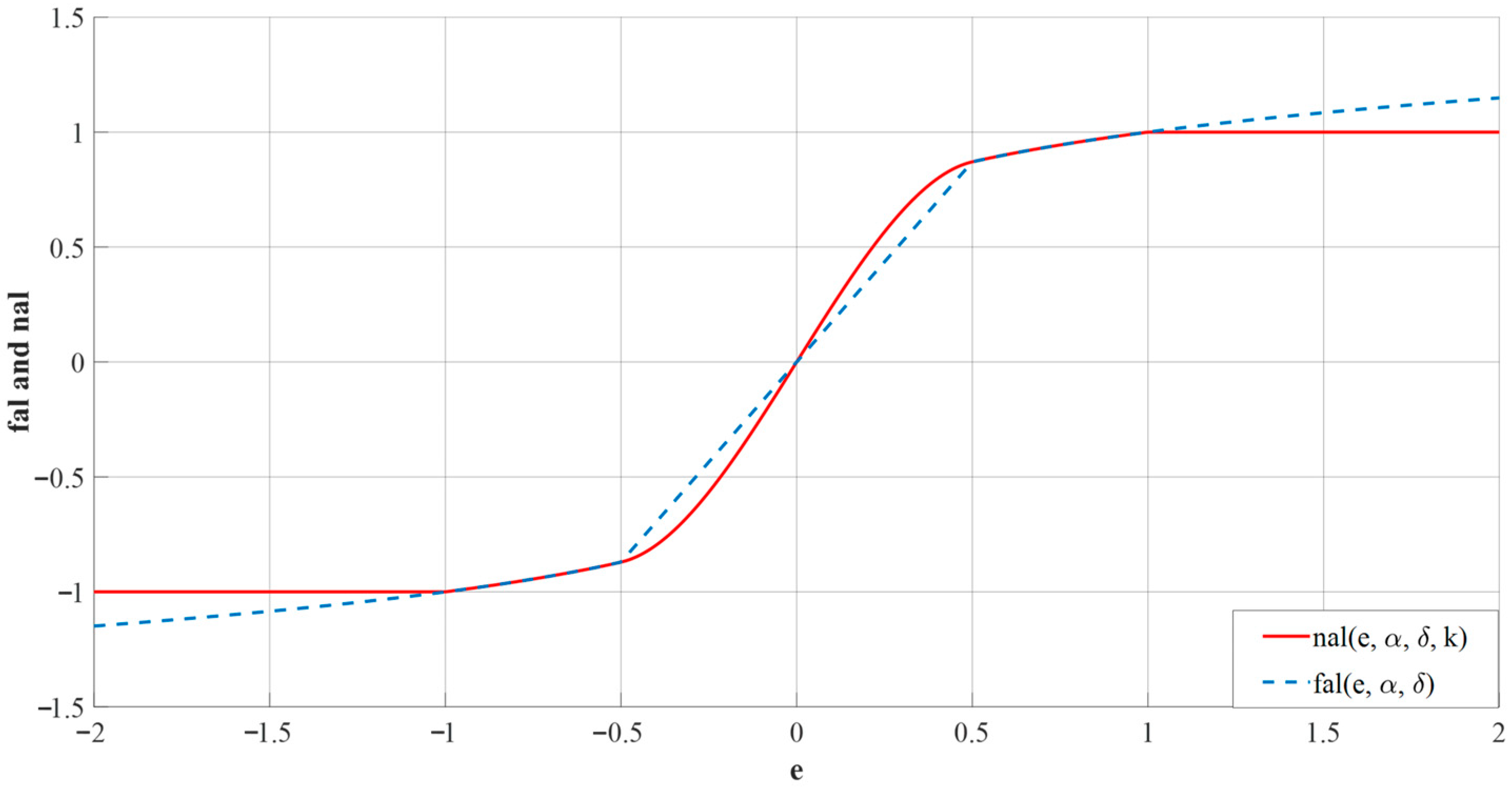
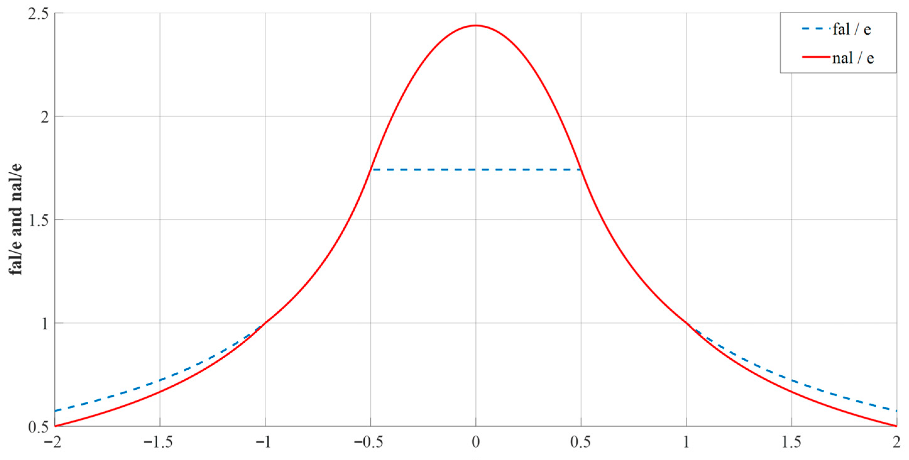
To validate the nonlinear function $nal(e,a,\delta ,k)$, simulations were conducted. When $\alpha =0.2$, $\delta =0.5$, and $k=1$, the characteristic curve simulation results for the traditional nonlinear function $fal(e,a,\delta )$ and the improved nonlinear function $nal(e,a,\delta ,k)$ are shown in Figure 4. The ratio of the function to the error e is termed the error gain; the error gain curves for both functions are depicted in Figure 5.

The core principle of deviation control lies in dynamically adjusting the control input based on the deviation between the system setpoint and actual output. This progressively reduces or eliminates the deviation, enabling the system output to gradually converge towards the desired trajectory. Self-disturbance-rejecting control operates precisely on this deviation adjustment mechanism. By continuously calculating the error between the reference input and actual output, it modifies the control quantity accordingly to suppress disturbances and optimise system performance.

Traditional ESO operates by tracking the system state variables $x_1$, $x_2$, and $x_3$ in real time through the system state variables $z_1$, $z_2$, and $z_3$. It adjusts the deviation e between $z_1$ and $x_1$ by modifying the derivative of $z_1$, adhering to the error principle. However, the tracking of system state variables by $z_1$, $z_2$, and $z_3$ follows a specific sequence. First, $z_1$ tracks $x_1$; next, $z_2$ tracks $x_2$; finally, $z_3$ tracks $z_3$. When $z_1$ completes tracking of $x_1$, the extremely small deviation e renders $z_2$ unable to track $x_2$ and $z_3$ unable to track $z_3$. At this point, substantial gains $l_2$ and $l_3$ would be required to complete tracking successfully. However, this operation would significantly impact the ESO’s performance, potentially causing oscillations or even system instability. Therefore, by calculating the deviation $e_2$ between $z_2$ and $x_2$, and the deviation $e_3$ between $z_3$ and $x_3$, these values serve as control quantities for $z_2$ and $z_3$, thereby enhancing the system’s convergence speed.

From Equation (5), the conventional ESO can be expressed as:

$$\left\{\begin{array}{l}{z}_1=e+x_1\hfill \\ z_2={\dot{z}}_1+l_{1}e\hfill \\ z_3=z_2+l_{2}f\mathrm{al}(e,{\alpha }_1,\delta )-b_{0}u\hfill \end{array}\right.$$

(11)

Based on Equation (4), it can be obtained that:

$$\left\{\begin{array}{l}{\dot{z}}_1={\dot{x}}_1+\dot{e}=x_2+\dot{e}\hfill \\ {\ddot{z}}_2={\ddot{z}}_1+l_1\dot{e}={\dot{x}}_2+\ddot{e}+l_1\dot{e}=x_3+\ddot{e}+l_1\dot{e}+b_{0}u\hfill \end{array}\right.$$

(12)

Substituting Equation (12) into Equation (11) yields:

$$\left\{\begin{array}{l}{z}_1=x_1+e\hfill \\ z_2=x_2+\dot{e}+l_{1}e\hfill \\ z_3=x_3+\ddot{e}+l_1\dot{e}+l_2\mathrm{fal}(e,{\alpha }_1,\delta )\hfill \end{array}\right.$$

(13)

From Equation (13), it can be observed that the deviation between $z_1$ and $x_1$ is $e$, the deviation between $z_2$ and $x_2$ is $\dot{e}+l_{1}e$, and the deviation between $z_3$ and $x_3$ is $\ddot{e}+l_1\dot{e}+l_2\mathrm{fal}(e,{\alpha }_1,\delta )$. Combined with $nal(e,a,\delta ,k)$, the reconstructed improved ESO is:

$$\left\{\begin{array}{l}e=z_1-x_1\hfill \\ {\dot{z}}_1=z_2-l_{1}e\hfill \\ {\dot{z}}_2=z_3-l_{2}n\mathrm{al}(\dot{e}+l_{1}e,{\alpha }_1,\delta ,k)+b_{0}u\hfill \\ {\dot{z}}_3=-l_3\mathrm{nal}(\ddot{e}+l_1\dot{e}+l_2\mathrm{nal}(e,{\alpha }_1,\delta ,k),{\alpha }_2,\delta ,k)\hfill \end{array}\right.$$

(14)

3.1.2. Stability Proof of the Improved ESO

Error Dynamics

The system state equations are given by (4):

$$\left\{\begin{array}{l}{\dot{x}}_1=x_2\hfill \\ {\dot{x}}_2=x_3-b_{0}u\hfill \\ {\dot{x}}_3={\dot{f}}_d(t)\hfill \end{array}\right.$$

(15)

Define the observation errors as $e_1=z_1-x_1$, $e_2=z_2-x_2$, $e_3=z_3-x_3$.

The improved ESO is described by:

$$\left\{\begin{array}{l}e=z_1-x_1=e_1\hfill \\ {\dot{z}}_1=z_2-l_{1}e\hfill \\ {\dot{z}}_2=z_3-l_{2}nal\left(\dot{e}+l_{1}e,{\alpha }_1,\delta ,k+b_{0}u\right)+b_{0}u\hfill \\ {\dot{z}}_3=-l_{3}nal\left(\ddot{e}+l_1\dot{e}+l_2\mathrm{nal}(e,{\alpha }_1,\delta ,k),{\alpha }_2,\delta ,k\right) \hfill \end{array}\right.$$

(16)

where $nal(\cdot )$ is the improved nonlinear function defined in (8), satisfying $0<{\displaystyle \frac{\mathrm{nal}(x)}{x}}\le k_f$ for $x\ne 0$.

From the structure, we observe that the inputs to the nonlinear functions represent the deviation control terms:

$${\epsilon }_2=\dot{e}+l_{1}e=(z_2-x_2)+l_1(z_1-x_1)=e_2+l_1{e}_1$$

(17)

$${\epsilon }_3=\ddot{e}+l_1\dot{e}+l_2\mathrm{nal}(e,{\alpha }_1,\delta ,k)={\dot{e}}_2+l_1{e}_2+l_2\mathrm{nal}(e_1)$$

(18)

These are precisely the error-based deviation quantities that accelerate convergence.

Subtracting the system dynamics from the observer dynamics and using the above relationships, the error dynamics can be derived as:

$$\left\{\begin{array}{l}{\dot{e}}_1=e_2-l_1{e}_1\hfill \\ {\dot{e}}_2=e_3-l_2\cdot {\displaystyle \frac{\mathrm{nal}({\epsilon }_2)}{{\epsilon }_2}}{\epsilon }_2\hfill \\ {\dot{e}}_3=-l_3\cdot {\displaystyle \frac{\mathrm{nal}({\epsilon }_3)}{{\epsilon }_3}}{\epsilon }_3-{\dot{f}}_d(t)\hfill \end{array}\right.$$

(19)

By defining ${\gamma }_2={\displaystyle \frac{\mathrm{nal}({\epsilon }_2)}{{\epsilon }_2}}$ and ${\gamma }_3={\displaystyle \frac{\mathrm{nal}({\epsilon }_3)}{{\epsilon }_3}}$, we have $0<{\gamma }_2,{\gamma }_3\le k_f$ from Assumption 2.

Matrix Form and Assumptions

The error system can be written in compact form:

$$\dot{E}=A(E)E+B{\dot{f}}_d(t)$$

(20)

where $E=[e_1,e_2,e_3{]}^T$,

$$A(E)=\left[\begin{array}{ccc}-l_1& 1& 0\\ -l_2{\gamma }_2& -l_2{\gamma }_2{l}_1& 1\\ -l_3{\gamma }_3(l_2{\gamma }_2)& -l_3{\gamma }_3(l_1+l_2{\gamma }_2{l}_1)& -l_3{\gamma }_3\end{array}\right], B=\left[\begin{array}{c}0\\ 0\\ -1\end{array}\right]$$

(21)

Note that the elements of $A(E)$ are bounded due to $0<{\gamma }_2,{\gamma }_3\le k_f$.

Assumption 1. 

${\dot{f}}_d(t)$ is bounded: $\mid {\dot{f}}_d(t)\mid \le M_1$.

Assumption 2. 

The nonlinear function satisfies $0<{\displaystyle \frac{\mathrm{nal}(x)}{x}}\le k_f$ for all $x\ne 0$.

Parameter Condition and Lyapunov Function

Choose observer gains satisfying:

$$l_1>0, l_2>{\displaystyle \frac{1}{l_1}}, l_3>{\displaystyle \frac{l_2}{l_1}}{k}_f$$

(22)

Construct the Lyapunov function $V(E)=E^{T}PE$ with:

$$P=\left[\begin{array}{ccc}{\displaystyle \frac{l_1^2+l_2+l_3}{2}}& {\displaystyle \frac{l_1}{2}}& {\displaystyle \frac{1}{2}}\\ {\displaystyle \frac{l_1}{2}}& 1& 0\\ {\displaystyle \frac{1}{2}}& 0& 1\end{array}\right]$$

(23)

Under condition (22), $P$ is positive definite.

Stability Analysis

Differentiating $V$ and substituting (20):

$$\dot{V}=E^T (A^{T}P+PA)E+2E^T PB{\dot{f}}_d(t)$$

(24)

Define $Q=-(A^{T}P+PA)$. It can be shown that under (22) and given the boundedness of ${\gamma }_2,{\gamma }_3$, the matrix $Q$ is positive definite for all $E$. Therefore,

$$\dot{V}\le -{\lambda }_{\min }(Q)\Vert E{\Vert }^2+2\Vert PB\Vert \Vert E\Vert |{\dot{f}}_d(t)|$$

(25)

Using Assumption 1 ($\mid {\dot{f}}_d(t)\mid \le M_1$) and letting $C=2\parallel PB\parallel M_1$:

$$\dot{V}\le -{\lambda }_{\min }(Q)\Vert E{\Vert }^2+C\Vert E\Vert =-\Vert E\Vert \left({\lambda }_{\min }(Q)\Vert E\Vert -C\right)$$

(26)

Hence, $\dot{V}<0$ whenever $\parallel E\parallel >C/{\lambda }_{\mathrm{m}\mathrm{i}\mathrm{n}}(Q)$, which implies that the observation errors are uniformly ultimately bounded.

When ${\dot{f}}_d(t)=0$, we obtain $\dot{V}\le -{\lambda }_{\mathrm{m}\mathrm{i}\mathrm{n}}(Q)\parallel E{\parallel }^2\le 0$, guaranteeing asymptotic stability of the origin.

3.1.3. Design of an ESO-Based Sliding Mode Controller

After estimating the system state and total disturbance via ESO, sliding mode control is employed to regulate the output voltage. The output voltage tracking error is treated as the state variable of the sliding surface, with the sliding surface selected as:

$$s=e+c{\displaystyle {\int }_0^{t}e}dt$$

(27)

where $e$ denotes the output voltage tracking error, $e=V_{ref}-U_o$, and $c>0$.

The derivative of the sliding surface is:

$$\dot{s}=\dot{e}+ce={\dot{V}}_{ref}-{\dot{U}}_o+ce=-f-b_{0}u+c(V_{ref}-U_o)$$

(28)

To accelerate the convergence speed of the system state, ensuring convergence within a finite time while mitigating chattering phenomena, an exponential convergence rate is employed in the design of the sliding mode controller.

$${\displaystyle \frac{ds}{dt}}=-\epsilon \mathrm{sgn}(s)-ks, \epsilon >0,k>0,$$

(29)

Traditional exponential approach law: When $\epsilon$ is set to a high value, the speed at which the sliding surface is reached increases, but this introduces significant chattering. When $\epsilon$ is set to a low value, chattering is suppressed, but the approach process is prolonged, resulting in slower dynamic response. To address this issue, this paper proposes an improved exponential approach law:

$$\begin{gathered} \dot{s}=-kG(s)s-\epsilon F(s)\tanh (s) \\ \left\{\begin{array}{l}G(s)=\ln (|s|+e)\hfill \\ \begin{array}{l}F(s)={\displaystyle \frac{|x|}{a|x|e^{|x|/b}+1/(|s|+1)}},\epsilon >0,k>0,a>1,b>0\\ \underset{t\to \infty }{\lim }|x|=0\end{array}\hfill \end{array}\right. \end{gathered}$$

(30)

where x denotes the system state variable; $\tanh (s)$ represents the hyperbolic tangent function, employed here as a continuous switching function; $\epsilon$ adjusts the convergence strength of the sliding surface S; k influences the global convergence rate; and e is the natural constant.

To demonstrate the stability of the sliding mode controller, the Lyapunov function is selected as:

$$V={\displaystyle \frac{1}{2}}{s}^2$$

(31)

Taking the derivative with respect to V and substituting into (26) yields:

$$\dot{V}=s\dot{s}=s\left[-kG(s)s-\epsilon F(s)\mathrm{sign}(s)\right]=-kG(s)s^2-\epsilon F(s)s\tanh \left(s\right)$$

(32)

Equation (32) satisfies: $G(s)>0, s^2>0, \mathrm{F}\left(s\right)>0, s·\tanh \left(s\right)>0$, yielding:

$$\dot{V}=-kG(s)s^2-\epsilon F(s)s\tanh (s)\le 0$$

(33)

where equality holds only when $s=0$. Hence, $\dot{V}$ is negative definite.

Thus, the system can reach the sliding surface within finite time. This indicates that the novel exponential convergence law not only guarantees the asymptotic stability of the system but also possesses the property of finite-time convergence.

From the preceding analysis, it follows that Equation (14) yields the estimated output voltage $z_1$ and the estimated total disturbance $z_3$. Thus, the control law can be expressed as:

$$u={\displaystyle \frac{1}{b_0}}\left[k\ln (|s|+e)s+\epsilon {\displaystyle \frac{|V_{ref}-U_o|}{a|V_{ref}-U_o|e^{\left|V_{ref}-U_o\right|/b}+\frac{1}{|s|+1}}}\tanh (s)+\mathrm{c}\left(V_{ref}-U_o\right)-f\right]$$

(34)

As analysed previously, the observer yields estimates $z_1$ for the output voltage $U_o$ and $z_3$ for the total disturbance. Consequently, the control law can be expressed as:

$$u={\displaystyle \frac{1}{b_0}}\left[k\ln (|s|+e)s+\epsilon {\displaystyle \frac{|V_{ref}-z_1|}{a|V_{ref}-z_1|e^{\left|V_{ref}-z_1\right|/b}+\frac{1}{|s|+1}}}\tanh (s)+\mathrm{c}(V_{ref}-z_1)-z_3\right]$$

(35)

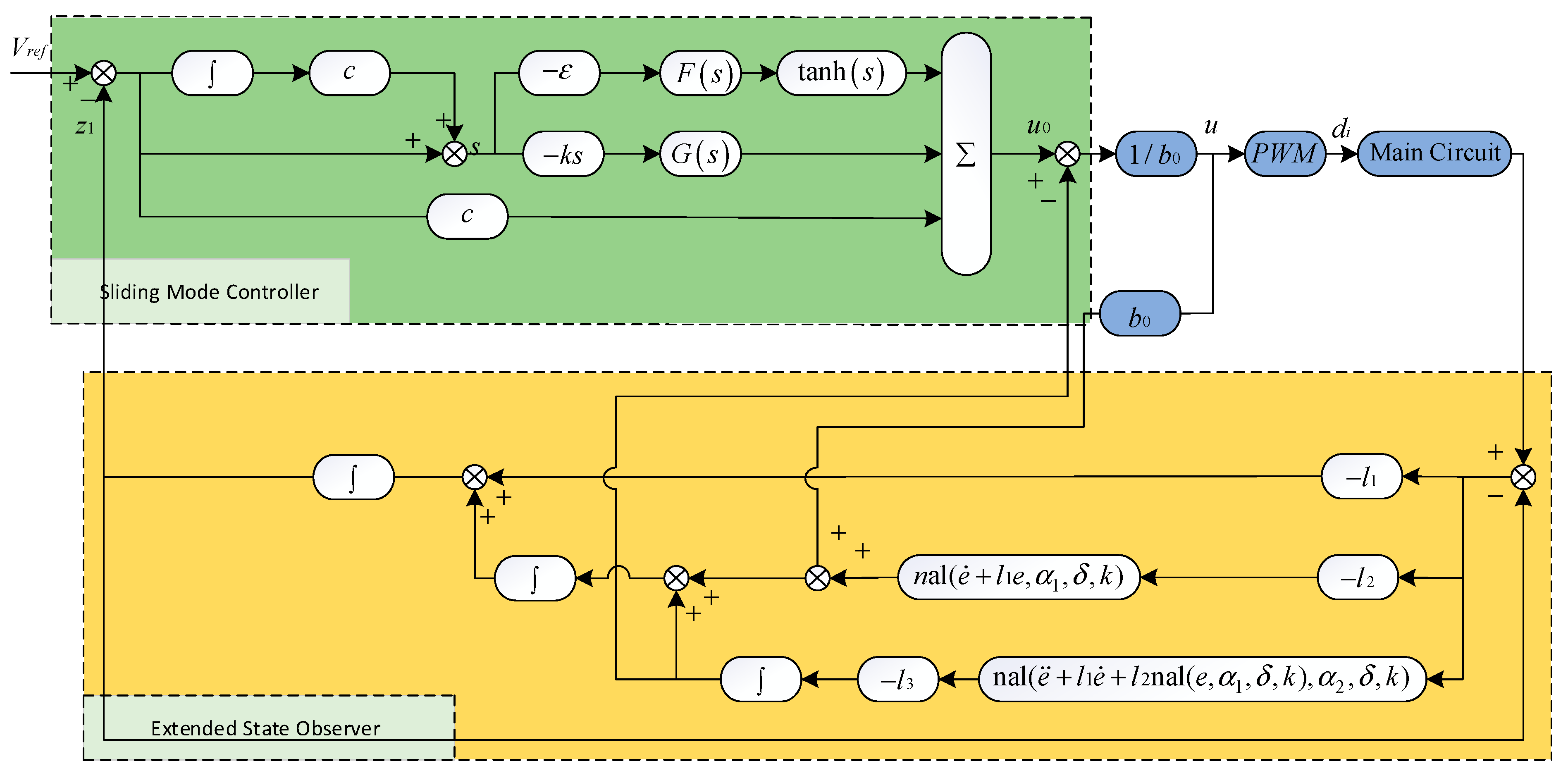
Equation (35) reveals that the sliding mode control law comprises an equivalent control term $u_{eq}={\displaystyle \frac{1}{b_0}}\left[c\left(V_{ref}-z_1\right)-z_3\right]$ and a switching control term $u_{sw}={\displaystyle \frac{1}{b_0}}\left[k\ln (|s|+e)s+\epsilon {\displaystyle \frac{|V_{ref}-z_1|}{a|V_{ref}-z_1|e^{\left|V_{ref}-z_1\right|/b}+\frac{1}{|s|+1}}}\tanh (s)\right]$. The equivalent control guides the system state towards the sliding surface, while the switching control maintains the system state in motion upon the sliding surface. The ESO observes system disturbances and feeds them back to the sliding mode controller, thereby reducing the sliding coefficients, alleviating the pressure on the sliding mode controller, suppressing controller chattering, and enhancing the system’s disturbance rejection capability. Figure 6 illustrates the designed voltage outer-loop control structure.

To validate the effectiveness of the proposed sliding mode control, simulation analysis is conducted using a typical second-order system as an example, referencing Equation (1). The system design is as follows:

$$\left\{\begin{array}{l}{\dot{x}}_1=x_2\hfill \\ {\dot{x}}_2=gu(t)+x_1+h(t)\hfill \end{array}\right.$$

(36)

The above equation assumes that the signals satisfy $g=10$, the disturbance signal is $h=10\sin (\pi t)$, $u(t)$ represents the controlled output, and $\theta$ denotes the position signal.

The sliding surface is defined as:

$$s=\dot{e}+ce$$

(37)

where $e$ denotes the position error and $\dot{e}$ denotes the position error rate of change, expressed as:

$$\left\{\begin{array}{l}e={\theta }_{ref}-\theta ,\hfill \\ \dot{e}={\dot{\theta }}_{ref}-\dot{\theta },\hfill \end{array}\right.$$

(38)

In the equation, ${\theta }_{ref}$ represents the desired position and $\theta$ denotes the actual position.

Combining Equations (36) to (38), we obtain

$${\displaystyle \frac{ds}{dt}}=c\left[{\dot{\theta }}_{ref}-\dot{\theta }\right]+\left[{\ddot{\theta }}_{ref}-\theta -gu(t)-h(t)\right]$$

(39)

Substituting Equation (30) into Equation (39) yields the output of the sliding mode controller

$$u(t)={\displaystyle \frac{1}{g}}\left[c\left({\dot{\theta }}_{ref}-\dot{\theta }\right)+{\ddot{\theta }}_{ref}-\theta -h(t)+k\ln (|s|+e)s+\epsilon {\displaystyle \frac{|x|}{a|x|e^{\left|x\right|/b}+\frac{1}{|s|+1}}}\tanh (s)\right]$$

(40)

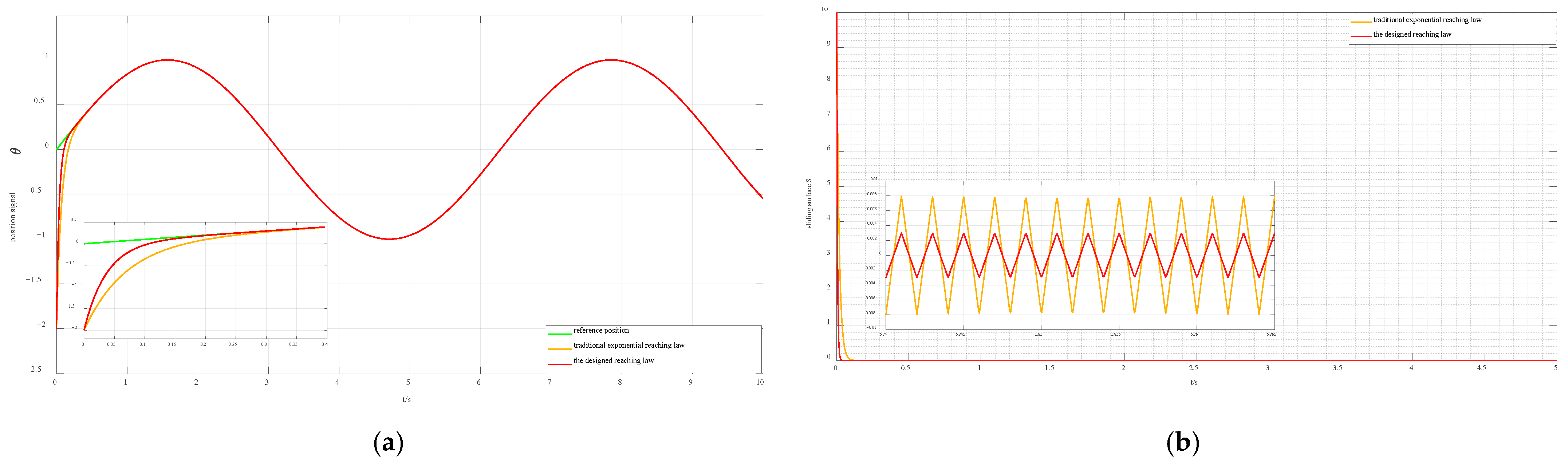
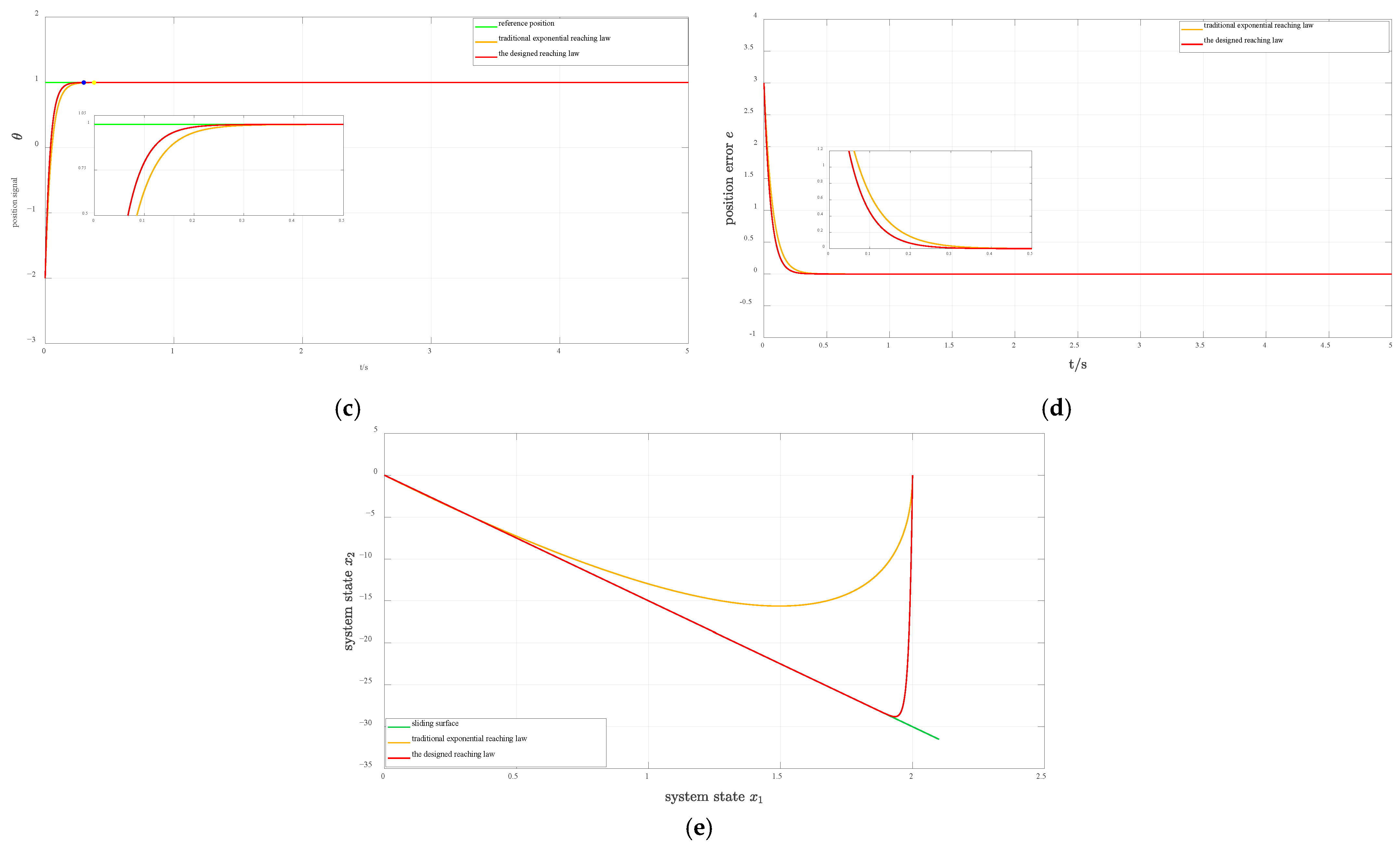
The initial value of the controlled object $x(0)$ is set to $[x_1, x_2] = [-2, -2]$. Simulation parameters are configured as follows: traditional exponential approach law control parameters: $\epsilon =12$, $k=25$, $c=15$; approach law control parameters designed in Section 3.1.3: $\epsilon =12$, $k=25$, $c=15$, $\alpha =2$, $b=6$. The desired system position ${\theta }_{ref}=\sin t$ and step signal are specified. The simulation comparison results for the approach laws are shown in Figure 7. Comparative analysis of dynamic responses under sinusoidal and step signals demonstrates that the proposed approach exhibits superior overall performance compared to traditional exponential approaches in terms of enhanced convergence speed, improved trajectory tracking accuracy, and effective suppression of system chatter.

4. Simulation Analysis

To validate the effectiveness of the proposed control strategy, a three-phase interleaved parallel buck converter was modelled in MATLAB/Simulink R2024a, which verified the correctness of the theoretical analysis while enabling a comparison of the dynamic performance of the proposed control, PI control, and conventional LADRC under identical circuit parameters. To ensure a fair comparison, all controllers were tuned using systematic methods with consistent design objectives. Specifically, the PI controller was tuned using the modulus optimum method, while the conventional ADRC and the proposed SM-ADRC share the same observer bandwidth ${\omega }_o=1200 \mathrm{rad}/\mathrm{s}$ and controller bandwidth ${\omega }_c=400 \mathrm{rad}/\mathrm{s}$, following the bandwidth parameterisation approach. For ADRC, the observer gains are set as ${\beta }_1=3{\omega }_o$, ${\beta }_2=3{\omega }_o^2$, ${\beta }_3={\omega }_o^3$; for SM-ADRC, the same bandwidth-parameterised gains $l_1=3{\omega }_o$, $l_2=3{\omega }_o^2$, $l_3={\omega }_o^3$ are used, together with sliding mode parameters $c=100$, $\lambda =500$, $k=0.1$, and $a=5$, selected to achieve a comparable closed-loop bandwidth. This consistent parameter selection ensures that any observed performance differences reflect structural advantages rather than tuning discrepancies. Due to space constraints, key circuit topology parameters are listed in

Table 2. Circuit topology parameters.

Parameter	Value
Output voltage reference value $V_{ref}$/$\mathrm{V}$	300
Phase Filter Inductor $L$/$\mathrm{mH}$	1.56
Filter capacitance $C$/$\mathsf{\mu }\mathrm{F}$	500
Switching frequency $f$/$\mathrm{kHz}$	100
Input voltage $U_{in}$/$\mathrm{V}$	750
Load $R$/$\Omega$	20

, while the control circuit parameters for all three strategies are summarised in

Table 3. Control circuit parameters.

Control Strategy	Voltage Outer Loop	Current Inner Loop
PI	$k_{pv}=0.5$	$k_{pi}=0.7$, $k_{ii}=6$
	$k_{iv}=150$
LADRC	$w_0=1200$, $b_0=9\times {10}^5$
	$w_c=400$
SM-ADRC	$w_0=1200$, $b_0=9\times {10}^5$
	${\alpha }_1=0.5$, ${\alpha }_2=0.25$
	$\delta =0.02$, $\epsilon =4$
	$k=50$, $c=260$
	$a=3$, $b=10$

.

The switching frequency is set to 100 kHz, which is typical for ZVS operation. The proposed SM-ADRC strategy, with its fixed-frequency PWM and interleaved structure, is inherently compatible with ZVS implementation. Recent studies, such as [26], have demonstrated the integration of advanced control with soft-switching in high-frequency converters. A detailed ZVS analysis is planned for future work.

4.1. Expected Voltage Step Change Comparison

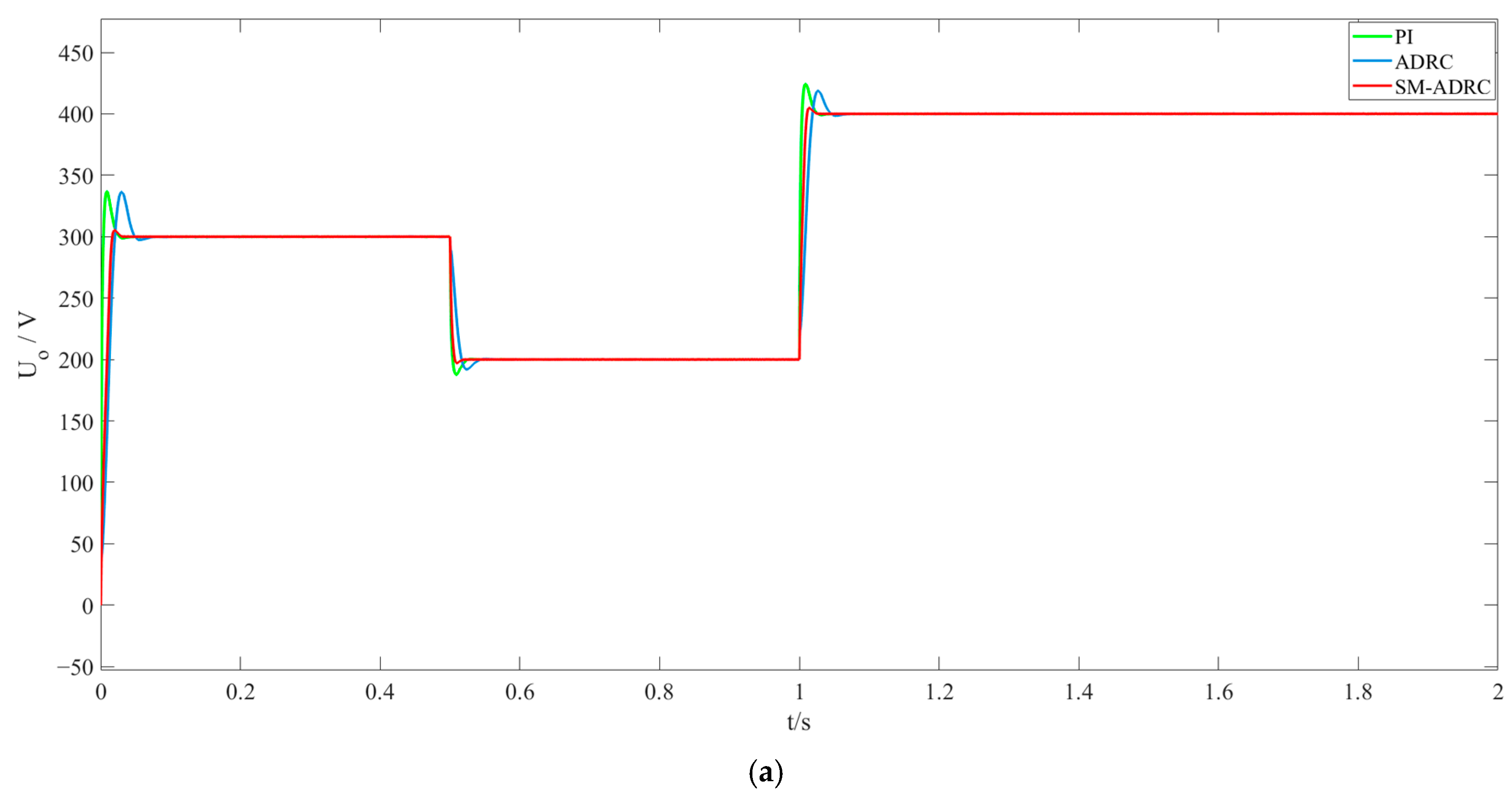
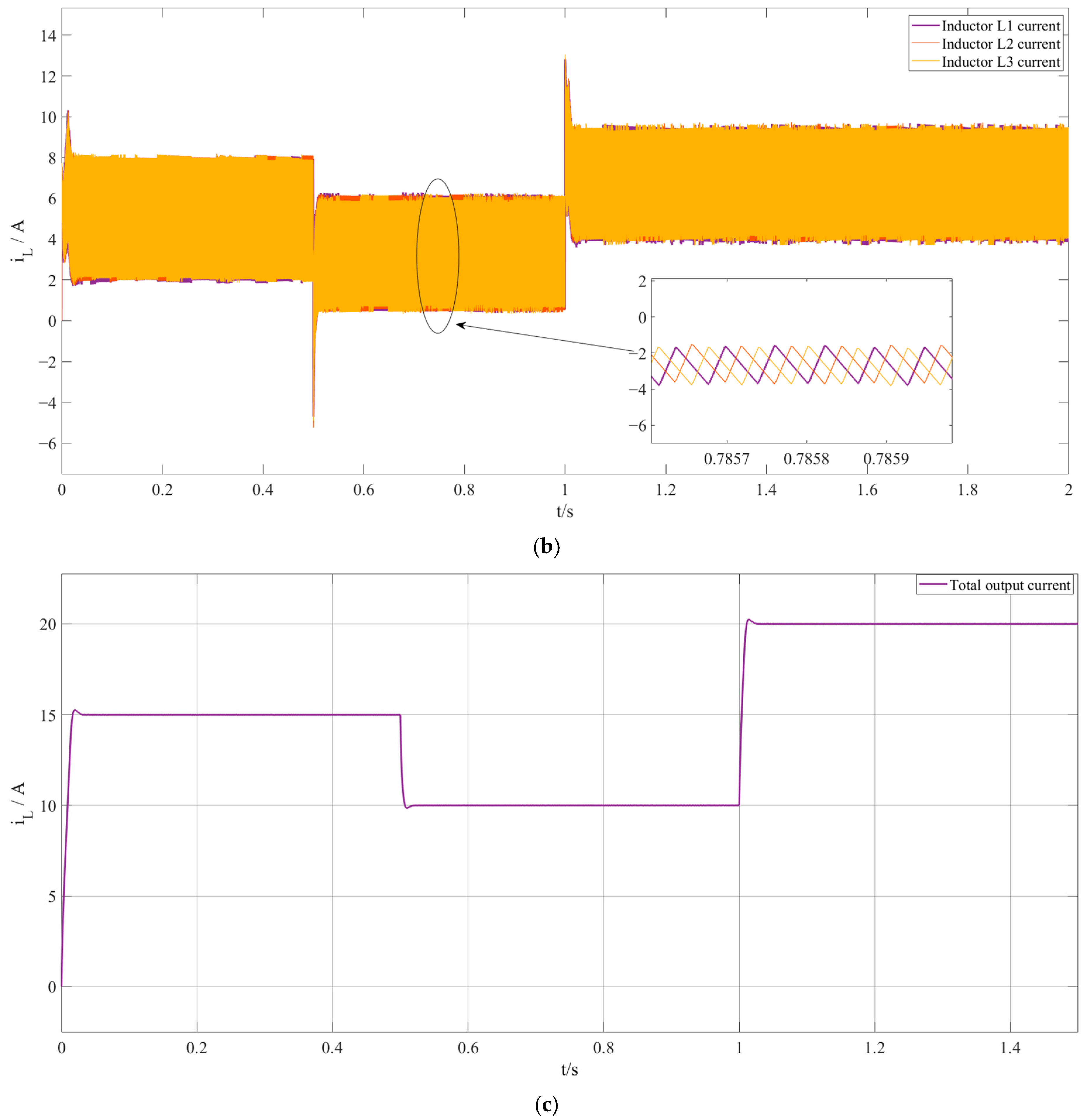
In the absence of other disturbances, an experiment was designed to compare desired output voltage step changes. The desired voltage was set to change sequentially from 300 V to 200 V and then to 400 V after 0.5 s. The control results are shown in Figure 8a. It can be observed that the output terminal can track the desired voltage system settings relatively quickly. Compared to traditional ADRC and PI control, the SM-ADRC exhibits a faster response speed and smaller steady-state error. Figure 8b and Figure 8c, respectively, illustrate the variations in three-phase interleaved inductor currents and output current during SM-ADRC. The results demonstrate effective current-sharing and rapid response during the control process.

4.2. Comparison of Load Disturbance Responses

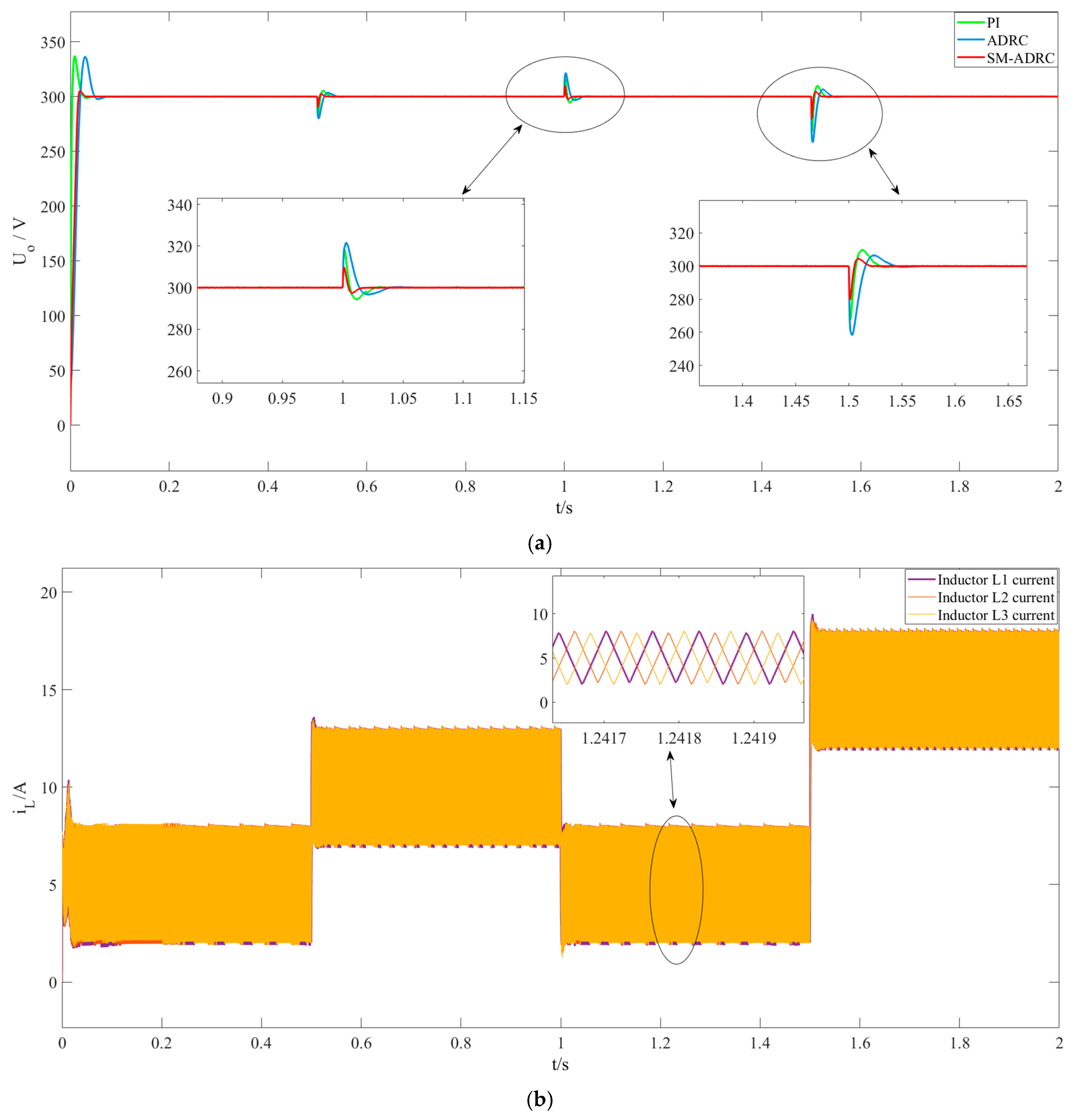
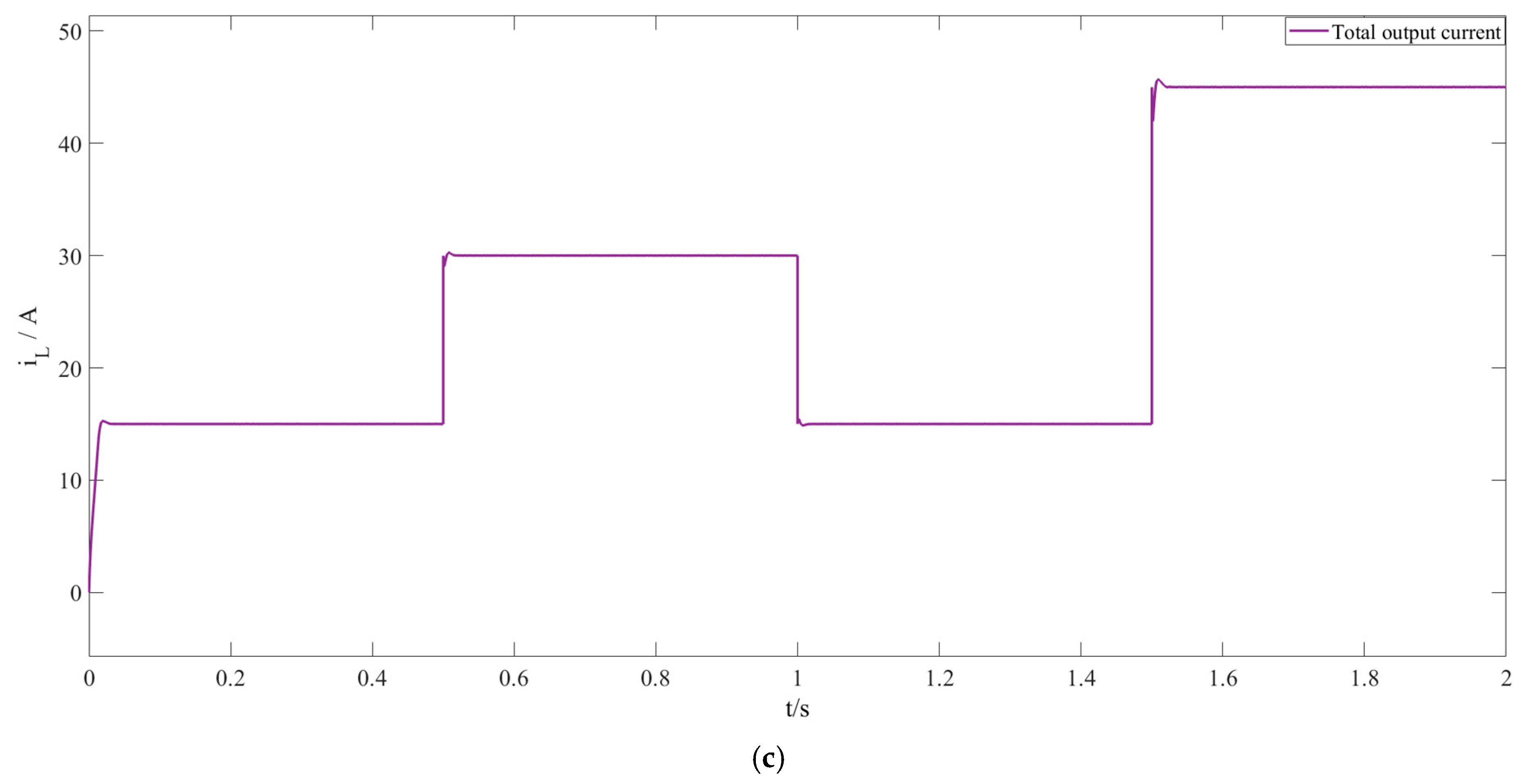
Considering load transients, the system’s disturbance immunity is verified. Load resistance $R$ was initially set to $20 \Omega$, abruptly changing every 0.5 s to $10 \Omega$, $20 \Omega$, and ${\displaystyle \frac{10}{3}} \Omega$. Results are shown in Figure 9a, exemplifying the 0.5 s load disturbance. When the load suddenly decreased to $10 \Omega$ at 0.5 s, the output voltage fluctuated. Under SM-ADRC, the peak voltage fluctuation reached 9.9 V with a recovery time of $18 \mathrm{ms}$. In contrast, under ADRC and PI control, peak voltage fluctuations were 20.2 V and 17.1 V respectively, with recovery times of $44 \mathrm{ms}$ and $39 \mathrm{ms}$. Figure 9b depicts the variation in three-phase interleaved inductor current during the SM-ADRC process. Following a load disturbance at 0.5 s, the load decreases while the input current correspondingly increases, satisfying the principle of energy conservation. Figure 9c illustrates the output current variation in SM-ADRC during three-phase interleaved parallel operation. The current response during control is observed to be relatively rapid. Consequently, under load transients, the proposed control strategy effectively suppresses voltage fluctuations, shortens recovery time, and demonstrates superior disturbance rejection performance.

4.3. Comparison of Input Voltage Disturbances

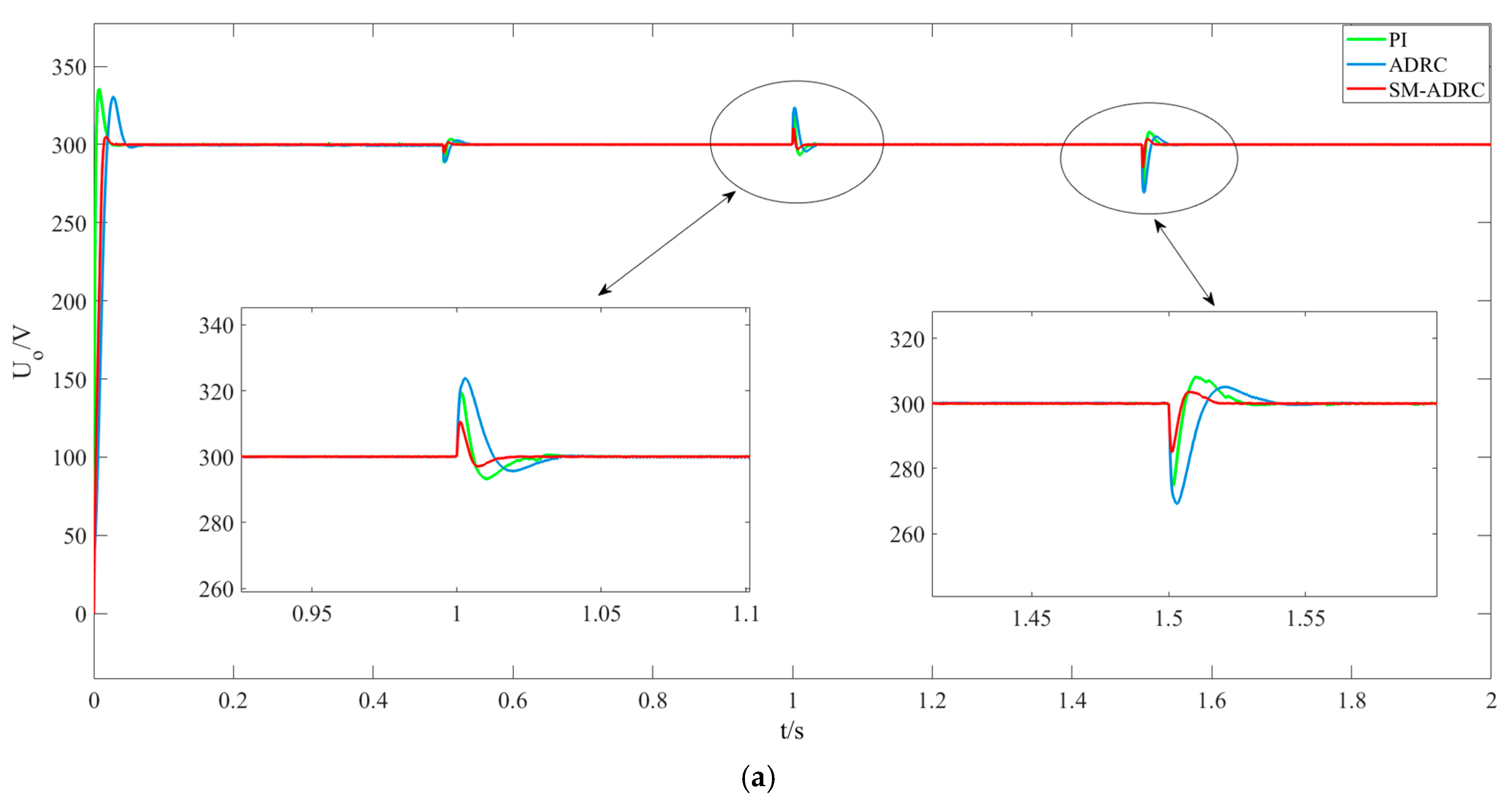
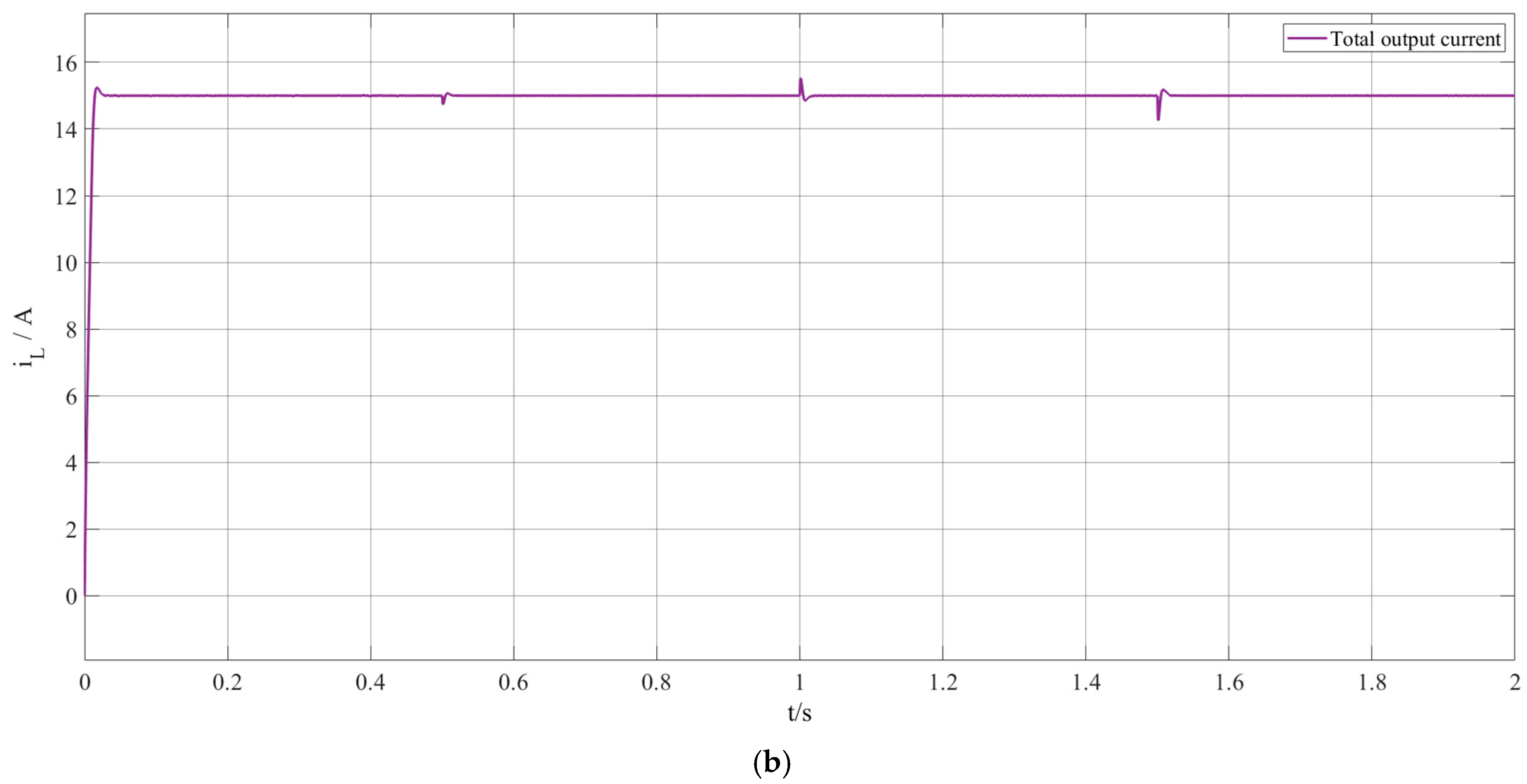
To compare the dynamic performance of the three control strategies under input voltage disturbances, the input voltage was abruptly stepped to 650 V, 850 V, and 600 V at 0.5 s intervals. The results are shown in Figure 10a, taking the input voltage disturbance at 0.5 s as an example. At 0.5 s, the input voltage abruptly changed from 750 V to 650 V, causing fluctuations in the output voltage. Under SM-ADRC, the peak output voltage fluctuation was 5.3 V, with a recovery time of $15 \mathrm{ms}$. Under PI and ADRC, the peak output voltage fluctuations were 11.6 V and 11.2 V, respectively, with recovery times of $31 \mathrm{ms}$ and $42 \mathrm{ms}$. The proposed control strategy demonstrated significant superiority over traditional ADRC and PI control strategies in terms of voltage overshoot and dynamic response speed.

To provide a more quantitative comparison of the three control strategies, the key performance metrics extracted from the simulation results are summarised in

Table 4. Quantitative performance comparison of three control strategies.

Disturbance Scenario	Performance Metric	PI	ADRC	SM-ADRC
Output voltage step change (300 V → 200 V)	Peak voltage fluctuation (V)	12.5	8.1	3.0
	Time to reach steady state (ms)	37	43	21
Load disturbance (20 Ω → 10 Ω)	Peak voltage fluctuation (V)	17.1	20.2	9.9
	Time to reach steady state (ms)	39	44	18
Input voltage disturbance (750 V → 650 V)	Peak voltage fluctuation (V)	11.6	11.2	5.3
	Time to reach steady state (ms)	31	42	15

.

5. Conclusions

This paper addresses the issue of fluctuating DC bus voltages in battery energy storage systems by proposing an enhanced SM-ADRC composite control strategy. Theoretical analysis and simulation comparisons validate the superiority of the proposed control strategy, yielding the following conclusions:

(1)

By modifying the nonlinear function in conventional ADRC and recalculating the deviation of the ESO state variable as the control input based on deviation control principles, the observer’s disturbance estimation accuracy and dynamic response speed are enhanced.

(2)

The modified state error feedback law employs integral sliding mode control to enhance robustness, while an improved exponential convergence rate mitigates steady-state degradation caused by chattering, thereby strengthening the disturbance rejection capability.

(3)

Comparative analysis of overshoot magnitude and duration under load and input voltage disturbances reveals that the proposed SM-ADRC strategy demonstrably outperforms conventional ADRC and PI control schemes in disturbance rejection and transient performance enhancement, exhibiting significant engineering applicability.

In addition to the performance improvements demonstrated in simulation, the proposed SM-ADRC strategy is designed with practical implementation in mind. The selected controller bandwidth $wc=400$ corresponds to a sampling frequency of $10 \mathrm{kHz}$, which is readily achievable with standard digital signal processors and leaves sufficient margin for computation. The improved ESO inherently estimates and compensates for total disturbances, including parameter mismatches and model uncertainties, thereby maintaining robustness under non-ideal conditions. The modified reaching law employs a continuous hyperbolic tangent function, which effectively reduces high-frequency switching noise compared to conventional sliding mode control. The additional computational burden introduced by the nal function and the hyperbolic tangent is moderate and well within the real-time capabilities of modern microcontrollers. Experimental validation on a hardware prototype is planned for future work to further substantiate the practical applicability of the proposed method.

References

1. Zhang, C.; Bao, Y.; Meng, X. Adaptive Virtual DC Motor Control for DC/DC Converters in DC Microgrid Energy Storage Systems. Power Syst. Prot. Control. 2023, 51, 12–20. [Google Scholar]
2. Zhang, Y.; Gong, R.; Liu, J. Fuzzy High-Order Sliding Mode Control for Three-Phase Interleaved Parallel DC–DC Converters. Control. Theory Appl. 2023, 40, 565–573. [Google Scholar]
3. Velmajala, K.; Sandepudi, S.R. High Step-Up Interleaved DC-DC Converter With Fault-Tolerant Capability. Int. J. Circuit Theory Appl. 2025, 53, 7214–7232. [Google Scholar] [CrossRef]
4. Oh, Y.G.; Choi, W.Y.; Kwon, J.M. Design of a Step-Up DC–DC Converter for Standalone Photovoltaic Systems with Battery Energy Storages. Energies 2021, 15, 44. [Google Scholar] [CrossRef]
5. Vijayan, M.; Udumula, R.R.; Mahto, T.; Kodumur Meesala, R.E. A novel multi-port high-gain bidirectional DC–DC converter for energy storage system integration with DC microgrids. J. Energy Storage 2024, 87, 111431. [Google Scholar] [CrossRef]
6. Wang, Z.; Wang, D.; Peng, Z.; Liu, L. Model-free adaptive control for ultracapacitor based three-phase interleaved bidirectional DC–DC converter. IET Power Electron. 2023, 16, 2696–2707. [Google Scholar] [CrossRef]
7. Zholtayev, D.; Rubagotti, M.; Do, T.D. Adaptive super-twisting sliding mode control for maximum power point tracking of PMSG-based wind energy conversion systems. Renew. Energy 2022, 183, 877–889. [Google Scholar] [CrossRef]
8. Ma, R.; Guo, X.; Zhang, Y.; Gui, J. PMSG offshore wind power system control using SMC and ADRC with fast SVPWM in complicated environment. Electr. Eng. 2023, 105, 2751–2767. [Google Scholar] [CrossRef]
9. Zhao, E.; Han, Y.; Liu, Y.; Yang, P.; Zalhaf, A.S.; Blaabjerg, F. An optimised parameter design of passivity-based controller for single-phase voltage source inverters. Int. J. Electr. Power Energy Syst. 2023, 145, 108627. [Google Scholar] [CrossRef]
10. Zheng, Y.; Cungang, H.; Tao, R. Model-free predictive voltage control strategy for LC-filtered voltage source inverter. Trans. China Electrotech. Soc. 2023, 38, 3723–3732. [Google Scholar]
11. Guochang, B.; Ke, L.; Chaoqun, M. Position control of permanent magnet synchronous motors based on improved self-disturbance rejection. Comb. Mach. Tools Autom. Mach. Technol. 2022, 10, 74–78. [Google Scholar]
12. Lanhong, Z.; Sheng, L.; Qingjie, Z. Design of Self-Disturbance-Rejecting Speed-Ring Controller for Permanent Magnet Synchronous Wind Power Systems. Control. Eng. 2022, 29, 1645–1651. [Google Scholar]
13. Wang, L.; Wu, Z.; Liu, Y.; Chen, Y. Research on Dual-Loop ADRC for PMSM Based on Opposition-Based Learning Hybrid Optimisation Algorithm. Algorithms 2025, 18, 559. [Google Scholar] [CrossRef]
14. Xinyu, Q.; Wenya, Z.; Guoqiang, W. Improvement of Self-Disturbance Rejection FAL Function and Its Application in Drag-Free Satellite. Aerosp. Control. 2022, 40, 38–44. [Google Scholar]
15. Xiao, Y.; Sun, C.; Lian, C. Research on tracking and synchronisation control of dual hydraulic cylinders based on improved active disturbance rejection control. Eng. Res. Express 2024, 6, 035513. [Google Scholar] [CrossRef]
16. Liao, Z.; Hao, Y.; Guo, T.; Lv, B.; Wang, Q. Second-order sliding mode control of permanent magnet synchronous motor based on singular perturbation. Energies 2022, 15, 8028. [Google Scholar] [CrossRef]
17. Pei, X.; Zhao, X.; Jia, H.; Wang, H.; Liu, J. Fuzzy sliding mode control with adaptive exponential reaching law for inverters in the photovoltaic microgrid. Front. Energy Res. 2024, 12, 1416863. [Google Scholar] [CrossRef]
18. Ma, B.; Jiao, J.; Ye, Z. Adaptive Fast Integral Terminal Sliding Mode Control Strategy Based on Four-Switch Buck–Boost Converters. Energies 2024, 17, 3645. [Google Scholar] [CrossRef]
19. Sun, C.; Dong, X.; Wang, M.; Li, J. Sliding mode control of electro-hydraulic position servo system based on adaptive reaching law. Appl. Sci. 2022, 12, 6897. [Google Scholar] [CrossRef]
20. Xu, B.; Sun, H.; Ji, W.; Ding, S.; Liu, T. An improved sliding mode speed controller for PMSM based on new terminal reaching law with generalised proportional integral observer. Trans. Inst. Meas. Control. 2024, 46, 2355–2366. [Google Scholar] [CrossRef]
21. Xu, B.; Zhang, L.; Ji, W. Improved non-singular fast terminal sliding mode control with disturbance observer for PMSM drives. IEEE Trans. Transp. Electrif. 2021, 7, 2753–2762. [Google Scholar] [CrossRef]
22. Hui, M.; Weitao, C.; Benling, Y.; Junbo, Z.; Lei, X. Research on Model Predictive Current Control for Three-Phase Hybrid Converters Based on Variable-Exponential Sliding Mode. Trans. Inst. Electr. Eng. 2025, 29, 75–84. [Google Scholar]
23. Ji, P.; Li, C.; Ma, F. Sliding mode control of manipulator based on improved reaching law and sliding surface. Mathematics 2022, 10, 1935. [Google Scholar] [CrossRef]
24. Jiang, J.; Zhang, H.; Jin, D.; Wang, A.; Liu, L. Disturbance observer based non-singular fast terminal sliding mode control of permanent magnet synchronous motors. J. Power Electron. 2024, 24, 249–257. [Google Scholar] [CrossRef]
25. Liu, Z.; Chen, W. Research on an improved sliding mode observer for speed estimation in permanent magnet synchronous motor. Processes 2022, 10, 1182. [Google Scholar] [CrossRef]
26. Zhu, G.; Dong, J.; Grazian, F.; Bauer, P. A hybrid modulation scheme for efficiency optimization and ripple reduction in secondary-side controlled wireless power transfer systems. IEEE Trans. Transp. Electrif. 2024, 11, 6840–6853. [Google Scholar] [CrossRef]
Figure 1. Topology of a three-phase interleaved parallel buck converter.
Energies 19 01846 g001
Figure 2. Equivalent circuit of buck converter.
Energies 19 01846 g002
Figure 3. Control principle of three-phase interleaved parallel buck converter.
Energies 19 01846 g003
Figure 4. Comparison of characteristic curves for traditional and improved nonlinear functions.
Energies 19 01846 g004
Figure 5. Comparison of error gain curves for traditional and improved nonlinear functions.
Energies 19 01846 g005
Figure 6. Voltage outer-loop control structure.
Energies 19 01846 g006
Figure 7. Simulation comparison of traditional approach law and designed approach law: (a) sine wave response under disturbance 10 sin ( π t ) ; (b) convergence test of sliding surface under; (c) step response under disturbance 10 sin ( π t ) ; (d) step error under disturbance 10 sin ( π t ) ; (e) sliding mode convergence rate for external disturbance signal.
Energies 19 01846 g007aEnergies 19 01846 g007b
Figure 8. Comparison of output voltage control and SM-ADRC-controlled inductor current changes during desired voltage step transitions. (a) Comparison of output voltage control during desired voltage transients; (b) three-phase inductor currents under SM-ADRC during desired voltage step changes; (c) output current under SM-ADRC during desired voltage step change.
Energies 19 01846 g008aEnergies 19 01846 g008b
Figure 9. Comparison of output voltage control and SM-ADRC-controlled inductor current variation during load disturbance. (a) Comparison of output voltage during load disturbance; (b) three-phase inductor current under load disturbance with SM-ADRC; (c) output current of SM-ADRC during load disturbance.
Energies 19 01846 g009aEnergies 19 01846 g009b
Figure 10. Control comparison of output voltage and variation in inductor current under SM-ADRC during input voltage disturbance. (a) Comparison of output voltage during input voltage disturbance; (b) output current under SM-ADRC during input voltage disturbance.
Energies 19 01846 g010aEnergies 19 01846 g010b