


Abstract
Improving the prediction accuracy of renewable energy power generation units is an important goal of the “source-storage integration” approach. However, the abundance of anomalous data and indistinct features in renewable energy station data seriously affects the health status prediction of these generator sets. To effectively enhance the performance of renewable energy generation prediction, this paper proposes an efficient data cleaning method for renewable energy stations based on anomaly detection and feature enhancement. First, anomaly detection is achieved by calculating a baseline power curve and partitioning data, utilizing the Density-Based Spatial Clustering of Applications with Noise (DBSCAN). Subsequently, considering that current models often learn low-frequency features while ignoring high-frequency features when processing time-series data, a data feature enhancement method is proposed. The proposed method integrates high-/low-frequency data decomposition, time–frequency domain conversion, and an improved attention mechanism to effectively enhance the high-frequency features of renewable energy station data, and reduces the RMSE of mainstream forecasting models significantly. Finally, using data from a renewable energy station in a region of China, the effectiveness and superiority of the anomaly detection and feature enhancement methods are analyzed. The results show that for renewable energy generation data, the proposed method reduces the RMSE of LSTM and Transformer models by 15.12%, 16.67% and 16.24%, 18.32% respectively, significantly improving prediction accuracy.
1. Introduction
1.1. Motivation
As a prominent representative of clean energy in source-storage power stations, renewable energy power generation is currently encountering novel challenges in the technologies for operational status monitoring and fault early warning [1]. Modern renewable energy units operate for long periods under complex meteorological conditions, and various system components are susceptible to performance degradation due to dynamic loads. This cumulative damage can significantly reduce power generation efficiency and increase operation and maintenance burdens. High-quality fan operation data is a core element for achieving intelligent operation and maintenance. However, actual data collected from renewable energy stations often contains various types of outliers: measurement deviations caused by sensor drift, packet loss during data transmission, and abnormal records caused by manual curtailment [2]. At the same time, the time-series characteristics of renewable energy station data further exacerbate the difficulty of data processing [3]. These data quality issues seriously interfere with the accuracy of key downstream algorithms. Therefore, robust data cleaning and preprocessing technologies are foundational prerequisites that provide reliable input for performance prediction models. Recent comprehensive reviews further emphasize that failing to effectively filter out these complex outliers can lead to cascading error propagation in subsequent predictive control systems [4].
1.2. Literature Survey
In the field of anomaly detection, current identification methods include traditional statistical methods (e.g., the 3σ rule and the quartile method) and machine learning-based approaches. However, traditional threshold methods adapt poorly to dynamic operating conditions due to their reliance on rigid boundaries. To overcome this, probabilistic and clustering methods have gained prominence. Zhao et al. [5] proposed a data-driven correction method combining the quartile method and Density-Based Spatial Clustering of Applications with Noise (DBSCAN) to identify abnormal data under wind curtailment conditions. Wang et al. [6] proposed a joint probability model based on Copula theory, rejecting abnormal data deviating from the wind power curve. Ciulla et al. [7] utilized multi-layer artificial neural networks to model actual wind power curves and identify abnormal operating states. Yesilbudak et al. [8] found that a hybrid model based on K-means and Smoothing Spline could significantly improve power curve modeling. Recent studies have further demonstrated that improving classic clustering algorithms, such as integrating dynamic parameters into DBSCAN or combining it with random forests, can effectively enhance anomaly identification under complex environmental conditions [9]. Despite these advancements, existing methods possess significant analytical limitations. Classic clustering algorithms (like standard DBSCAN) suffer from severe boundary sensitivity when processing high-dimensional, nonlinear time-series data. Specifically, in a renewable energy scatter plot, the data density is highly non-uniform (sparse above the theoretical curve, extremely dense below). Applying a single, global parameter set to such data inevitably leads to high false-positive rates in sparse regions and high false-negative rates in dense regions.
In terms of feature enhancement and forecasting following data cleaning, methods such as Convolutional Neural Networks (CNNs), One-Dimensional CNNs (1DCNNs), Temporal Convolutional Networks (TCNs), and attention mechanisms have been extensively studied [10,11,12,13]. Ren et al. [14] constructed a CNN-LSTM model with an attention mechanism to achieve joint feature extraction. Furthermore, Transformer-based architectures, relying on their powerful self-attention mechanisms, have increasingly become a mainstream approach for handling complex spatiotemporal correlations in renewable energy generation forecasting [15]. To handle data volatility, decomposition-based hybrid models have become popular. Xiong et al. [16] proposed a hybrid model combining Complementary Ensemble Empirical Mode Decomposition (CEEMD), Bidirectional LSTM (BiLSTM), and Extreme Learning Machines. Geng et al. [17] developed a method based on Wide First-Layer Kernel Deep CNNs (WDCNNs) and stacked BiLSTMs to extract temporal correlations. Furthermore, Ding et al. [18] and Zhu et al. [19] successfully applied decomposition algorithms like CEEMD combined with optimization algorithms for short-term prediction. However, a critical limitation remains: deep learning forecasting models inherently suffer from “frequency bias” [20]. When processing highly volatile data, models tend to aggressively learn low-frequency macroscopic trends (which dominate the loss function) while simultaneously smoothing out and ignoring high-frequency microscopic features (small amplitude fluctuations). Because renewable generation relies heavily on short-term weather dynamics, ignoring these high-frequency components causes critical information loss and severely degrades forecasting accuracy.
Current methodologies treat anomaly detection and forecasting feature extraction as isolated tasks, failing to systematically connect the macroscopic density imbalance of anomalies with the microscopic frequency bias of forecasting models. To bridge this gap, rather than presenting a broad conceptual overhaul, this paper provides a targeted engineering methodology. We argue that the optimal solution requires decoupling these problems: first, overcoming the boundary sensitivity of anomaly detection through local-density adaptation; second, directly counteracting the forecasting model’s frequency bias by explicitly forcing the network to assign weights to high-frequency components before forecasting.
1.3. Our Contributions
Therefore, this paper proposes an efficient data cleaning and enhancement method tailored for renewable energy stations. The main contributions are as follows:
- (1)
- Adaptive Partitioned Anomaly Detection: Targeting the macroscopic nonlinear density variations in renewable energy data, the Improved DBSCAN algorithm is proposed. By constructing a baseline power curve and utilizing adaptive data partitioning, the density thresholds are dynamically adjusted according to local data density, thereby mitigating the boundary sensitivity defects.
- (2)
- Decoupled High-/Low-Frequency Feature Enhancement: Addressing the microscopic “frequency bias” in traditional time-series forecasting, a feature enhancement method integrating high–low-frequency decomposition, time–frequency conversion, and an improved attention mechanism is proposed. This forces the network to enhance high-frequency dynamic features that are typically ignored.
- (3)
- Empirical Validation: Based on actual operation data from a renewable energy station in a region of China, the effectiveness of the proposed sequential methodology is verified, demonstrating a significant reduction in prediction errors.
2. Anomaly Data Detection Theory
2.1. Renewable Energy Generator Characteristics Analysis
The ultimate goal of renewable energy generation is to convert wind energy and solar energy into electrical energy [21]. The principles of photovoltaic power generation output are as follows.
wherein Pm represents the actual power generation, Pm* represents the rated power generation, G is the global incident radiation intensity on the surface of the photovoltaic module, G* is the standard incident radiation intensity on the surface of the photovoltaic module, Tc is the temperature of the battery, Tc* is the battery temperature under standard conditions, and represents the power temperature coefficient.
The principles of wind power generation output are as follows.
wherein P represents the power generation; ρ is the air density; y denotes the wind speed; Cp is the power coefficient; and R is the rotor radius.
There is a direct relationship between wind power/solar power generation output and wind speed/solar radiation.
Therefore, a scatter plot based on wind speed/solar radiation vs. renewable energy power can intuitively display whether the unit is abnormal. Through the wind speed/solar radiation vs. renewable energy power scatter plot, this paper first sorts out the abnormal data types of renewable energy stations, as shown in Figure 1. According to the operating status of the renewable energy generator set, outliers are divided into three types, with typical characteristics as follows:
Figure 1.
The abnormal data types. (a) Wind power farm; (b) solar power farm.
Anomaly Type 1: This type of abnormal data generally appears as a straight line in the wind speed/irradiance-power scatter plot, showing no power output at high wind speeds/irradiance, i.e., downtime/outage periods implemented by the operator.
Anomaly Type 2: These anomalies are characterized by a continuous and stable output of positive power below/above the rated power of the generating equipment, i.e., power curtailment implemented by the operator.
Anomaly Type 3: These anomalies are randomly distributed in the feature space. These anomalies may be caused by sensor faults or noise in signal processing [22]. These instances may also be generated by transitions from stop to run or vice versa, and such situations are best classified as anomalies.
2.2. Improved DBSCAN Clustering Algorithm
The distribution characteristics of renewable energy power and wind speed indicate that the distribution density of normal data in the feature space is significantly higher than that of abnormal samples, which provides a direction for distinguishing the two using the DBSCAN algorithm. The DBSCAN algorithm can utilize the differences existing between the two types of data to achieve effective partitioning and identification, without relying excessively on specific parameter settings, reducing dependence on prior knowledge to a certain extent, and reserving flexible space for subsequent model optimization.
-neighborhood: Within a radius of , the neighborhood of an object p is defined as the set of all objects q for which the distance between p and q is less than or equal to . Its formal definition is
where denotes the neighborhood of object p, represents the distance between p and q, is the radius threshold, and D is the dataset.
- (1)
- Core object: An object p is defined as a core object if the number of points contained in its -neighborhood is greater than or equal to the minimum number of points Z:
- (2)
- Directly density-reachable: In the dataset D, if an object p lies within the -neighborhood of an object q, and q satisfies Equation (3) (i.e., q is a core object), then the object q is said to be directly density-reachable from the object p.
- (3)
- Density-reachable: For a given radius and minimum number of points Z, if there exists a chain of objects such that and , and for any adjacent pair pi and pi+1 in the chain, pi+1 is directly density-reachable from pi with respect to and Z, then the object q is said to be density-reachable from the object p with respect to and Z.
- (4)
- Density-connected: If there exists an object such that both object p and object q are density-reachable from object , then the objects p and q are said to be density-connected with respect to and Z.
- (5)
- Clusters and noise: An arbitrary object is selected from the dataset D. Starting from this object p, all points satisfying the threshold Z and the property of density-reachability are searched to form a cluster. Any object that is not contained in any cluster is defined as noise.
As shown in Figure 1, in the wind speed–power scatter plot, the density distribution of abnormal data above the power curve differs from that below it. While the traditional DBSCAN algorithm can effectively identify outliers outside irregularly shaped clusters via density-based clustering, it has notable defects when processing the operational data of renewable energy power stations with highly uneven density distribution. The core logic of the DBSCAN algorithm (As shown in Figure 2) lies in determining the category of data points based on their density. Points of the same category tend to cluster closely, resulting in relatively short distances between any two points of the same category. Points that are density-connected are grouped into the same cluster, thereby achieving the clustering goal, and all points are classified based on their connectivity.
Figure 2.
A schematic diagram of DBSCAN clustering.
In the wind speed–power (irradiance-power) scatter plot, the data distribution density exhibits inherent significant heterogeneity determined by the physical characteristics of the generating units. The core logic is as follows: The power output of renewable energy units has clear physical boundaries. Wind power output is determined by wind speed, exhibiting a cubic relationship with wind speed from the cut-in wind speed to the rated wind speed, and maintains rated power after reaching the rated wind speed. Photovoltaic output shows an approximately linear positive correlation with irradiance; once the irradiance is determined, the theoretical maximum output of the unit is also determined. Therefore, the normal operating data of the units must be highly concentrated in the region near and below the theoretical rated power curve. This portion accounts for over 85% of the total samples and exhibits extremely high distribution density. In contrast, the region above the curve exceeds the physical output limit of the units and contains only a very small number of anomalous outliers caused by sensor faults or measurement noise, with extremely sparse distribution and a minimal number of samples. Furthermore, even within the region below the curve, there exists significant density heterogeneity: normal operating data closely adhering to the theoretical power curve are highly densely distributed, while curtailment anomalies and shutdown anomalies, located far from the curve, are scattered only in local areas, with an overall density far lower than that of the normal data concentration zone.
This inherent density heterogeneity, determined by physical characteristics, is precisely the core bottleneck of the traditional DBSCAN algorithm with globally fixed parameters—a single global density threshold cannot simultaneously adapt to regions with vastly different densities, making it highly prone to the issues of false detections of normal data and missed detections of anomalous data.
Therefore, the original operational data can be divided into the “above-curve dataset” and the “below-curve dataset” to make the density distribution of abnormal data in each subset more uniform, reducing the interference of density differences across regions on clustering. In the division principle, this paper divides the power data into equal intervals (2% of the installed capacity in this study), calculates the average wind speed data for each power interval, and then constructs a benchmark power curve using linear interpolation.
Subsequently, the DBSCAN model is applied to the two subsets separately, using Euclidean distance to measure the closeness between samples. The “density-reachable” relationship is defined through Eps (neighborhood distance threshold) and MinPts (minimum number of samples in the neighborhood) to avoid identification deviations caused by a single parameter adapting to all data. The maximum density-connected sample set is derived, and data points outside the set are identified as abnormal data. Finally, by merging the abnormal identification results of the two subsets, the final list of abnormal data is obtained.
The Eps and MinPts of traditional DBSCAN are globally fixed values, which cannot adapt to the density differences between the two subsets. This paper proposes a parameter adaptation strategy based on local density. The specific formulas and steps are as follows:
Calculate the local densities (above the curve) and (below the curve) for the two subsets. The local density is defined as
where Ni is the number of data points in the subset; Si is the distribution area of the subset in the wind speed–power space. The calculation method is as follows.
For all samples within the subset, determine the boundaries of the feature space: the range of the independent variable (wind speed/irradiance) is [xmin, xmax], and the range of the dependent variable (power) is [ymin, ymax].
Using an equally spaced grid division, the two-dimensional feature space is divided into grid cells with a resolution of 100 × 100.
Count the number of grid cells M that contain at least one sample point. Combined with the area of a single grid cell, the total distribution area of the subset is calculated as Si = M × Δx × Δy, where Δx and Δy are the step sizes of a single grid cell in the dimensions of the independent variable and dependent variable, respectively.
For the value of Eps, this paper uses the K-distance method (K = 5) to calculate the initial Eps for subset 2 (dense subset): draw the K-distance graph, and take the distance corresponding to the curve’s inflection point as Eps2. The specific process and determination criteria are as follows.
- (1)
- For each sample point within the dense subset D2, calculate its Euclidean distance to all other sample points in the subset. After sorting the distances in ascending order, the K-th distance is taken as the K-distance of that sample (based on sensitivity analysis validation, this paper adopts K = 5, which yields the optimal overall performance).
- (2)
- Sort the K-distances of all samples in descending order and plot the K-distance curve.
- (3)
- Elbow point determination criterion: The Savitzky–Golay filter (with a window length of 51 and polynomial order of three) is applied to smooth the K-distance curve, eliminating the interference of random noise on the identification of the elbow point. The second derivative of the smoothed curve is calculated, and the point corresponding to the maximum value of the second derivative is taken as the elbow point. This elbow point represents the transition point where the K-distance changes from gradual to steep. The samples before the transition point are densely distributed normal operating data, while the samples after the transition point are sparsely distributed anomalous data. Therefore, the K-distance value corresponding to this elbow point is taken as Eps2. Figure 3 visually illustrates the determination process of Eps2.Figure 3. K-distance curve and Eps inflection point identification.
For subset 1 (sparse subset), Eps is adjusted inversely proportional to the density to ensure that the neighborhood range in the sparse region is sufficient to cover normal data points and avoid misclassification.
where and are the local densities of the sparse subset and the dense subset, respectively. The core logic of this formula is as follows: the sparser the data distribution in a region, the larger the neighborhood radius required to ensure that the neighborhood of a core object contains enough sample points, thereby avoiding the misclassification of normally sparse distributed data as noise points; conversely, in densely distributed regions, a smaller neighborhood radius is adopted to accurately identify local anomalous samples and prevent missed detections.
The adaptive adjustment strategy for the Eps parameter in this paper follows the logic of “first determine a baseline, then adaptively adjust.” The underlying mechanism and calculation sequence are as follows.
- (1)
- Prioritize the denser subset D2 (the subset below the curve), which has a larger sample size and represents the majority of normal operating data, as the baseline. The K-distance method is used to determine Eps2. This is because the dense subset contains most of the normal operating data, and the elbow point feature of its K-distance curve is more pronounced, enabling a more accurate determination of the neighborhood range baseline for normal data and avoiding parameter deviations that could arise if the sparse subset were used as the baseline.
- (2)
- Density-based adaptive adjustment: Based on the ratio of local densities of the two subsets, Eps is inversely adjusted to obtain Eps1 for the sparse subset. For densely distributed regions, the distances between normal samples are smaller, so a smaller Eps is required to distinguish local outliers. For sparsely distributed regions, the distances between normal samples are inherently larger; if the same small Eps as used in dense regions were applied, a large number of normal samples would be misclassified as noise. Therefore, the Eps threshold needs to be adaptively amplified according to the density difference.
- (3)
- Role of overall data density: The overall data density affects the overall distribution of the K-distance curve, thereby influencing the value of the baseline parameter Eps2. Meanwhile, the relative density ratio between the two subsets determines the adjustment magnitude of Eps1 relative to Eps2, addressing the core issue that the traditional DBSCAN with a globally fixed parameter cannot adapt to density variations.
Regarding the MinPts value, it is defined as follows: if the number of samples contained within the ε-neighborhood of a sample is ≥MinPts, the sample is identified as a core object. Only samples identified as core objects can serve as the centers of clusters, incorporating density-reachable samples into the normal data set. In contrast, samples that cannot be covered by any core object are ultimately identified as anomalies (noise). Therefore, MinPts, as the core threshold for core object determination, directly dictates the accuracy of anomaly detection.
Traditional DBSCAN uses a globally fixed MinPts, which fails to adapt to the density differences between the two subsets obtained after partitioning in this paper: If MinPts is adapted to the sparse subset, it would cause numerous stacked curtailment anomalies within the dense subset to be misjudged as core objects and subsequently incorporated into the normal data, leading to severe missed detections. Conversely, if MinPts is adapted to the dense subset, it would prevent normal ramp-up data within the sparse subset from forming core objects, causing them to be misjudged as anomalies and resulting in severe false detections.
To address this core deficiency, this paper designs an adaptive calculation formula for MinPts based on the relative relationship between local density and global density. This allows the threshold to adjust dynamically according to the density characteristics of each subset, thereby ensuring the validity of core objects.
where is the adjustment coefficient (taken as 1.2), and its function is to perform an overall calibration of the threshold for core object determination, thereby avoiding excessive fragmentation of clusters caused by an excessively small MinPts value. is the total number of original data points, and [ ] denotes rounding up. This formula ensures that the dense subset has a larger MinPts, preventing densely distributed abnormal points from being misclassified as core objects.
The essence of MinPts in DBSCAN is the criterion for determining the “density of samples within a neighborhood.” Using the total number of samples in the entire dataset Ntotal as a global anchor ensures that the density determination rules for both sparse and dense subsets are completely unified and consistent. This prevents the issue of the judgment scales becoming decoupled or the criteria becoming fragmented between the two subsets after processing them separately, thereby ensuring fairness and consistency in anomaly detection.
By substituting Equation (5) into Equation (7), it can be concluded that the essence of MinPtsi is αNtotal/Si, and Ntotal ultimately forms a matching relationship with the distribution area Si of the subset. This design ensures that the value of MinPts is entirely determined by the actual distribution range of the data in the feature space, rather than by the number of samples. It precisely aligns with the distribution characteristics of “wide dispersion in sparse regions and high concentration in dense regions,” enabling adaptive adjustment of the parameter.
In practical application, for the dense subset, its data are highly concentrated in the feature space, resulting in a smaller distribution area Sᵢ (i.e., larger ρi). The formula thus yields a larger MinPtsᵢ, significantly raising the threshold for core object determination. Consequently, only points with sufficiently dense neighborhoods are identified as core objects, effectively preventing densely distributed curtailment-type anomalies from being misjudged as core objects and substantially reducing missed detections. For the sparse subset: its data are more widely dispersed in the feature space, resulting in a larger distribution area Sᵢ (i.e., smaller ρi). The formula thus yields a smaller MinPtsᵢ, appropriately lowering the threshold for core object determination. This allows the normally sparse ramp-up data to form valid core objects and clusters, preventing normal data from being misjudged as anomalies and significantly reducing false detections.
The above process can be summarized as Algorithm 1.
| Algorithm 1. Adaptive DBSCAN Anomaly Detection Based on Baseline Power Curve Partitioning |
| Input: 2D renewable energy dataset D = {(xi, pi)}, rated power Pr Output: Abnormal sample set O, Normal sample set N //Step 1: Build baseline power curve and partition dataset 1: Divide power range into equal intervals with Δp = 0.02 × Pr, 2: For each interval, calculate the average wind speed/irradiance to obtain the baseline curve f(x) via linear interpolation. 3: Split D into sparse subset D1 (pi ≥ f(xi), above curve) and dense subset D2 (pi < f(xi), below curve) //Step 2: Calculate local density of each subset 4: For each subset Di (i = 1, 2): 5: Divide its 2D feature space into 100 × 100 grids, count occupied grid number Mi 6: Compute distribution area Si = Mi × Δx × Δp, local density ρi = |Di|/Si 7: End for //Step 3: Adaptive calculation of DBSCAN core parameters 8: Compute baseline Eps2 for D2 via K-distance method (K = 5): get K-distance curve, smooth with SG filter, take elbow point value as Eps2 9: Calculate adaptive Eps1 = Eps2 × ρ2/ρ1 for sparse subset D1 10: For each subset Di: compute adaptive MinPtsi = ⌈α × ρi × |D|/|Di|⌉ (α = 1.2) 11: End for //Step 4: Block-wise DBSCAN and result merging 12: Run standard DBSCAN on D1 (Eps1, MinPts1) and D2 (Eps2, MinPts2), get abnormal subsets O1, O2 13: Merge abnormal set O = O1 ∪ O2, raw normal set Nraw = D\O 14: Fill gaps in Nraw via linear interpolation to get final normal set N 15: return O, N; |
3. Data Feature Enhancement Theory
3.1. Analysis of the Frequency Learning Bias Issue in Time Series Forecasting
After completing the cleaning of anomalous data, renewable energy power time-series data still exhibit strong non-stationarity and high volatility. However, existing mainstream time-series forecasting models (such as LSTM and Transformer) commonly suffer from a frequency learning bias issue. Specifically, during training, these models tend to prioritize learning low-frequency trend features from the data while inadequately learning high-frequency weak features that characterize short-term, sharp fluctuations in power output. This ultimately leads to over-smoothed forecasting results that fail to capture the abrupt change characteristics of wind and solar power, significantly limiting improvements in forecasting accuracy.
Taking the Transformer forecasting model as an example, a Discrete Fourier Transform is applied to the wind power forecasting results, yielding a frequency-domain distribution comparison between the predicted and actual values, as shown in Figure 4. It is clearly observable that the model achieves a good fit for low-frequency components below 2 × 10⁻⁵ Hz, with the spectral amplitudes of the predicted values closely matching the actual values. However, for high-frequency components above 1 × 10⁻⁴ Hz, the model’s learning effectiveness is extremely poor, with the spectral amplitudes of the predicted values being significantly lower than the actual ones, indicating a severe loss of high-frequency information.
Figure 4.
Comparison of the frequency domain of the Transformer prediction results. (a) Wind power prediction results and (b) solar power prediction results.
This frequency learning bias issue is one of the core challenges in the current field of wind and solar power forecasting. Existing research predominantly focuses on improving the structure of forecasting models or achieving separate predictions for multiple components through signal decomposition. However, these approaches do not design specialized enhancement mechanisms for high-frequency weak features and thus cannot fundamentally resolve the model’s low-frequency preference problem.
To address this, this chapter proposes a data feature enhancement theory. The core idea is as follows: First, wavelet packet decomposition is employed to accurately separate the high-frequency and low-frequency components of the time-series data. Subsequently, a Discrete Fourier Transform is used for time–frequency domain conversion, and a frequency-domain channel attention mechanism is designed to specifically enhance the weights of high-frequency features. This is then combined with a cross-temporal and cross-dimensional dual-channel attention module to achieve synergistic enhancement of spatiotemporal features. Finally, through an inverse transform, the enhanced output of time-domain features is obtained, fundamentally solving the model’s frequency learning bias problem and improving the feature representation capability of the data and the subsequent forecasting accuracy.
3.2. Wavelet Packet Decomposition-Based Separation of High- and Low-Frequency Features
Current prediction models predict large data changes relatively accurately, but are almost insensitive to small fluctuations. From a frequency domain perspective, after the Fourier Transform, existing models are sensitive to low-frequency features but insensitive to high-frequency features. The existing literature demonstrates that decomposing non-stationary time series into sub-sequences via wavelet packet transform can significantly improve a model’s ability to capture this high-frequency volatility [23]. Wavelet packet decomposition is an improvement based on the wavelet transform, which can decompose both low-frequency signals and high-frequency signals, enabling better time–frequency localization analysis for signals containing medium and high-frequency information.
For the wind and solar power time-series data with a 17 min sampling interval in this study, the high-frequency and low-frequency features are clearly defined based on the sampling frequency and the physical meaning of the signals:
Low-frequency features: Refer to signal components with frequencies below 1 × 10⁻⁴ Hz. These primarily characterize long-term trend features such as diurnal and seasonal variations in wind and solar power, as well as the slowly varying characteristics of wind speed and irradiance. These signal components have large amplitudes and strong regularity, making them the parts that traditional forecasting models learn most easily.
High-frequency features: Refer to signal components with frequencies above 1 × 10⁻⁴ Hz. These primarily characterize short-term dynamic characteristics such as sudden changes in wind speed, abrupt fluctuations in irradiance, and short-term output fluctuations of generating units. These signal components have small amplitudes, weak regularity, and a low signal-to-noise ratio. They are the core parts that traditional forecasting models learn insufficiently, and are also key to determining whether a forecasting model can capture power ramps.
Based on the above definitions, this study employs a six-layer wavelet packet decomposition to partition the original time-series signal into 64 equal-width sub-bands. Based on the center frequency of each sub-band, the low-frequency and high-frequency sub-bands can be accurately identified and distinguished, laying the foundation for the subsequent targeted feature enhancement.
The decomposition and reconstruction methods based on wavelet packets are as follows: Equation (8) is the decomposition process, and Equation (9) is the reconstruction process.
where and are the wavelet packet decomposition coefficients, and are the low-pass and high-pass filter banks in the wavelet packet decomposition process, respectively, and and are the low-pass and high-pass filter banks in the wavelet packet reconstruction process, respectively.
Through wavelet packet decomposition, the original time-series signal x(t) is decomposed into 26 = 64 sub-band components with equal bandwidth, each corresponding to a different frequency interval. Based on the aforementioned definition of high and low frequencies, all sub-band components are divided into a low-frequency component set and a high-frequency component set.
3.3. Time–Frequency Joint Dual-Channel Attention Feature Enhancement Module
3.3.1. DFT-Based Time–Frequency Domain Conversion Method
To enable the model to better learn the frequency domain characteristics in the high/low-frequency data of renewable energy, the Discrete Fourier Transform (DFT) is adopted to decompose the input time series into a frequency series. Subsequently, the frequency series is refined and normalized to prevent the model from focusing excessively on low-frequency components with large amplitudes. For example, for a given input sequence xl, the DFT can be expressed as
where ak represents frequency domain data, fk represents frequency data, k = 1, 2, …, l, and l is the data length.
3.3.2. Cross-Temporal Attention-Based Feature Enhancement
Since renewable energy data possesses strong volatility and periodicity, viewing it from a global perspective may likely ignore its important feature information. Therefore, to enhance its ability to extract local information features, slice segmentation and embedding are adopted to convert the input data into a sequence. This also converts the input one-dimensional data into a format suitable for the encoder.
In slice segmentation and embedding, the input signal is divided into N slices, and there are overlapping regions between the divided slices. The overlap between different slices enhances the feature extraction capability of the entire input signal. For the N-th slice, we overlap its end with the beginning of the first slice. As the slicing operates, each slice block is equivalent to an input [24]. In this way, the length of the input sequence decreases, which can greatly reduce computational volume and video memory usage.
For the N overlapping slices divided, with slice length L and overlap rate r = 0.3, the k-th slice is defined as
where the first and last slices satisfy (head–tail overlap), ensuring temporal continuity.
The self-attention mechanism is the core part of the Transformer, allowing the model to compare each element in the input sequence with other elements when processing the sequence. It enables the model to consider all elements in the sequence simultaneously, establishing dependencies between elements by calculating attention weights as shown in Equation (12).
where Q represents the query matrix, K represents the key matrix, V represents the value matrix, and dk represents the dimension.
Multi-head attention allows the model to jointly process information from different representation subspaces at different positions, used to enhance the model’s ability to model different relationships in the input sequence. It further improves the model’s expressive ability by applying the self-attention mechanism to multiple sets of different query matrices Q, key matrices K, and value matrices V. Its calculation process is shown in Equation (13).
For wind power and photovoltaic power generation data, the spatial and temporal dimensions have a crucial impact on the results. Multiple variables, such as wind speed, temperature, and air pressure, not only follow their own temporal evolution patterns but also have spatial coupling correlations. Recent advancements in deep learning have demonstrated that decoupling and jointly modeling these spatial and temporal dependencies through dedicated attention modules can significantly reduce forecasting errors under highly volatile weather conditions [25]. Traditional time-series modeling methods mostly rely on self-attention mechanisms to mine features along a single time dimension, which has inherent limitations in capturing spatio-temporal coupling correlations. In contrast, the cross-temporal attention mechanism adopted in this paper can collaboratively model temporal and spatial dependencies, and simultaneously capture the cross-temporal dynamic evolution and cross-dimensional correlation features of the data. And through joint spatio-temporal attention calculations, construct a three-dimensional interactive modeling framework to precisely analyze the cross-temporal correlations and enhance the representation ability of the dynamic evolution of wind power generation systems. Its structure is shown in Figure 5.
Figure 5.
Cross-temporal attention structure diagram.
The cross-temporal attention mechanism first captures the long-term dependencies in the time series through the self-attention mechanism in the temporal dimension. This process can be expressed as
where LayerNorm(·) represents layer normalization, MLP(·) represents the feedforward network, (·) represents the multi-head attention mechanism, where all dimensions are shared, and and represent the output of the and MLP.
Then, in the spatial dimension, the correlation between different variables is captured through the cross-dimensional attention mechanism. The process can be expressed as
where shares each point in time.
3.3.3. Frequency-Domain Channel Attention Mechanism
At the same time, to ensure independent computation of sub-band features and avoid learning bias, the attention mechanism proposed in Section 3.3.2 is designed to focus more on the feature correlations within each frequency component itself. A channel attention mechanism is adopted within the sub-frequency band, enabling the model to focus on learning the correlation between different channels within the same sub-frequency band, rather than amplitude differences between different frequency components.
For the n-th sub-frequency band, its cross-channel characteristic is expressed as
where m represents the number of channels, N represents the total number of frequency blocks, and denotes the characteristic of the m-th channel in the nth frequency block.
The channel self-attention calculation for the n-th frequency block is
where , , are the weight matrices for generating the query (Query), key (Key), and value (Value) matrices, respectively. d is the scaling factor for the attention score, which alleviates the problem of vanishing gradients in Softmax due to excessive inner product; represents the normalized cross-channel features of the nth frequency block.
Discrete Fourier Transform (DFT) is performed on the high-frequency component xh(t) and the low-frequency component after wavelet packet decomposition to obtain high-frequency frequency domain features Xh(f) and low-frequency frequency domain features. Targeting the high-frequency frequency domain features Xh(f), a channel attention mechanism is designed to strengthen the weight of the high-frequency band(f > 1 × 10⁻⁴ Hz):
where σ is the Sigmoid function, MLP is a two-layer perceptron, Wc is the channel attention weight, and is the enhanced frequency domain feature.
Finally, after achieving feature enhancement of the frequency domain signal, the frequency sequence is converted back to the time domain signal through Inverse Discrete Fourier Transform (IDFT) and denormalization. By utilizing Equation (9) for wavelet packet reconstruction of the high-frequency data time domain signal and the low-frequency data time domain signal, feature enhancement of renewable energy data is realized.
3.3.4. Implementation Process of the Feature Enhancement Method
The implementation process of the feature enhancement method proposed in this study is as follows:
- (1)
- Separation of high- and low-frequency features: The input time-series data is decomposed using a six-layer wavelet packet decomposition with the db9 wavelet basis. The low-frequency and high-frequency components are identified and separated, achieving effective separation of high- and low-frequency features.
- (2)
- Time–frequency domain conversion: The Discrete Fourier Transform is applied separately to the separated low-frequency and high-frequency components to convert the time-domain signals into frequency-domain sequences, obtaining the frequency-domain characteristics of each component.
- (3)
- Frequency-domain feature enhancement: For the frequency-domain features of the high-frequency components, a frequency-domain channel attention mechanism is employed to adaptively enhance the weights of weak high-frequency features, improving their representational capability. Simultaneously, the frequency-domain features of the low-frequency components are optimized synchronously to preserve core trend information.
- (4)
- Signal reconstruction and output: The enhanced high- and low-frequency time-domain components are reconstructed using a wavelet packet reconstruction algorithm to synthesize the complete feature-enhanced time-series data, which serves as the input for the subsequent power forecasting model.
Through the aforementioned complete process, the feature enhancement method proposed in this study achieves full-process processing from high–low-frequency separation and high-frequency feature enhancement to time-domain feature optimization. It is deeply integrated with the front-end anomaly detection module, collectively forming an integrated data cleaning framework for renewable energy (As shown in Figure 6).
Figure 6.
Overview of the data enhancement framework.
It should be clarified that the data cleaning proposed in this study refers to a broad, full-process data quality improvement framework. It encompasses not only the front-end detection and elimination of anomalous data (data cleaning in a narrow sense) but also the back-end stage of data feature enhancement. The core objective of both stages is identical: to improve the quality and usability of data from renewable energy stations, thereby providing higher-quality input for downstream tasks such as power forecasting and condition monitoring.
Specifically, the anomaly detection stage addresses the issue of erroneous values in the data. By eliminating anomalous data, it resolves problems related to incorrect and invalid samples, ensuring the fundamental authenticity and reliability of the data. The feature enhancement stage, on the other hand, tackles the issue of weak features. By strengthening the high-frequency weak features within the data that are difficult for models to learn, it enhances the data’s feature representation capability and resolves the learning bias problem in downstream models. Essentially, this stage represents a further optimization and improvement of data quality and is an indispensable core component of the broad data cleaning process.
4. Case Analysis
4.1. Data Source and Evaluation Metrics
The dataset for this paper comes from a region in China, containing six items of data: wind speed, wind direction, temperature, air pressure, relative humidity, and historical renewable energy power. The data collection period is from 1 January 2020 to 31 December 2021, with a sampling interval of 17 min.
To address the strong temporal autocorrelation of renewable energy power time series, this study strictly adheres to the principle of forward temporal partitioning. The training set comprises time-series data from 1 January 2020 to 30 June 2021, totaling 92,880 samples, accounting for 75% of the total sample size, and is used for model parameter training and learning. The validation set consists of time-series data from 1 July 2021 to 30 September 2021, totaling 15,552 samples, representing 12.5% of the total sample size, and is used for hyperparameter tuning to prevent model overfitting. The test set includes time-series data from 1 October 2021 to 31 December 2021, totaling 15,408 samples, accounting for 12.5% of the total sample size, and is completely excluded from model training and hyperparameter tuning, serving solely for final generalization testing of model performance.
In addition, we have established core protocols for model training. First, during the training process, if the loss value on the validation set does not decrease for ten consecutive epochs, early stopping is triggered to terminate training and save the optimal model parameters, thereby preventing overfitting. Second, all comparative experiments are independently repeated ten times with different random seeds, and the mean and standard deviation (SD) of the evaluation metrics across the ten runs are recorded to mitigate the impact of random initialization on experimental results. To verify whether the performance improvement of the proposed method is statistically significant, we adopt the two-tailed paired Student’s t-test for statistical verification. The test is performed on the 10 repeated experimental results of the proposed method and each baseline method, with the significance level set as follows: * p < 0.05 indicates a statistically significant difference between the two methods; ** p < 0.01 indicates an extremely statistically significant difference. Finally, all experiments are conducted on a device configured with an Intel i5-12490F CPU, NVIDIA RTX 3070 8G GPU, and 16G RAM. The programming environment is based on PyTorch 1.10.2 and Python 3.9, with the operating environment maintained consistently across all compared models.
In the anomaly detection analysis, to comprehensively and objectively evaluate the performance of the method, this paper adopts three core evaluation metrics commonly used in the field of anomaly detection: Precision, Recall, and F1 Score. These three metrics are all calculated based on the four fundamental elements of the Confusion Matrix: True Positive (TP): Real anomalous sample points correctly identified as anomalies by the model: False Positive (FP): Real normal sample points misjudged as anomalies by the model (false detections); True Negative (TN): Real normal sample points correctly identified as normal by the model; False Negative (FN): Real anomalous sample points misjudged as normal by the model (missed detections).
Based on the above four fundamental elements, the calculation formulas and physical meanings of the three core evaluation metrics are shown in Table 1. Among them, Precision reflects the proportion of samples judged as “anomalies” by the model that are truly anomalous, measuring the false detection rate of the anomaly detection model. The higher the precision, the fewer misjudgments of normal data by the model. Recall reflects the proportion of all real anomalous samples that are correctly identified by the model, measuring the missed detection rate of the anomaly detection model. The higher the recall, the more complete the model’s identification of anomalous data, and the fewer missed detections. The F1 Score is the harmonic mean of precision and recall, which can comprehensively measure the overall performance of the model and address the trade-off between precision and recall. The higher the F1 Score, the better the balance the model achieves between “reducing false detections” and “reducing missed detections,” and the better its overall performance.
Table 1.
Evaluation index.
In the final effect evaluation, to demonstrate the improvement effect of this method on power generation forecasting, this study adopts three metrics—Root Mean Square Error (RMSE), Mean Absolute Error (MAE), and Mean Squared Error (MSE)—for comprehensive assessment. RMSE amplifies the impact of larger errors through squaring, reflecting the overall deviation degree of prediction results; MAE directly calculates the average absolute deviation between predicted values and actual values, intuitively reflecting the average prediction accuracy of the model; MSE reinforces the weight of large error terms by squaring the errors, helping to identify the model’s performance in extreme situations. These three metrics assess the accuracy and stability of the prediction model from different angles, where RMSE is sensitive to outliers, MAE is more robust, and MSE focuses more on the impact of larger errors (The specific calculation formula is shown in Table 2). Through the synergistic analysis of these three metrics, the performance characteristics of the model in different prediction scenarios can be fully grasped.
Table 2.
Evaluation index.
4.2. Analysis of Anomaly Detection Effects
To systematically validate the anomaly detection performance of the partitioned adaptive DBSCAN algorithm proposed in this paper and comprehensively evaluate the effectiveness of the core components of data cleaning, this section conducts a complete experimental analysis from three perspectives: sensitivity analysis of core parameters, overall quantitative performance comparison, and visualization result validation. This quantitatively verifies the proposed method’s ability to identify anomalous data in renewable energy stations and its algorithm’s robustness.
4.2.1. Sensitivity Analysis of Core Parameters
The K value in the K-distance method is the core hyperparameter that determines the neighborhood radius threshold Eps of DBSCAN, directly influencing the accuracy and robustness of the anomaly detection model. Referring to the general setting rules for the DBSCAN algorithm in a two-dimensional feature space (wind speed/irradiance vs. active power), as well as relevant research in the field of anomaly detection for renewable energy power curves, this paper selects a reasonable range of K values (3, 4, 5, 6, and 7) to conduct a one-factor sensitivity analysis.
In the experiments, other parameters were fixed, and the precision, recall, and F1 Score of anomaly detection were used as evaluation metrics. Comparative validation was performed on two datasets—wind power and photovoltaic power—to quantitatively analyze the impact of different K values on model performance and to verify the rationality and cross-scenario generalizability of selecting K = 5 in this paper. The comparison results of model performance under different K values are shown in Table 3.
Table 3.
Comparison of anomaly detection performance under different K values.
It can be seen from the results that, in both the wind power and photovoltaic power scenarios, the trend of model performance with varying K values is consistent. As the K value increases, the F1 Score of anomaly detection initially increases and then decreases. When K = 5, the F1 Score reaches its maximum in both scenarios, indicating that the model achieves optimal overall performance.
When the K value is too small, the model becomes overly sensitive to local random noise, tending to misclassify normal random power fluctuations as anomalies, which leads to a decrease in precision. When the K value is too large, the model becomes insensitive to locally dense, stacked curtailment/abandonment anomalies, making it prone to missed detections of anomalies and resulting in a decrease in recall.
The correction factor α is a core parameter in the adaptive calculation formula for MinPts, used to perform an overall calibration of the core object determination threshold and to prevent excessive fragmentation of clusters caused by an excessively small MinPts. In this study, the baseline value of α is set to 1.2. To verify the rationality of this value and the robustness of the parameter, a reasonable range of α values [0.8, 1.0, 1.2, 1.4, 1.6] was selected for a one-factor sensitivity analysis. With other parameters fixed, the F1 Score of anomaly detection was used as the core evaluation metric. The experimental results on the wind power and photovoltaic power datasets are shown in Table 4.
Table 4.
Comparison of anomaly detection performance under different α values.
It can be observed from the experimental results that as the value of α increases, the precision of anomaly detection initially increases and then decreases, while the recall shows a continuous decreasing trend, with the F1 Score reaching its maximum at α = 1.2. When the α value is too small, the MinPts threshold is relatively low, making it easy to misclassify anomalies in dense regions as core objects, leading to a decrease in precision. When the α value is too large, the MinPts threshold is relatively high, making it easy to misclassify normal data in sparse regions as anomalies, resulting in a significant decrease in recall. At α = 1.2, the model achieves an optimal balance between precision and recall, with the highest F1 Score, verifying the rationality and optimality of this value.
4.2.2. Overall Quantitative Performance Evaluation of Anomaly Detection
To directly and quantitatively validate the core performance of the proposed anomaly detection method, this paper constructs a validation dataset with ground truth labels by manually labeling normal/anomalous samples with the assistance of experts in the field of renewable energy power systems.
The experiment employs three core evaluation metrics commonly used in the field of anomaly detection—precision, recall, and F1 Score—to conduct a quantitative comparison between the partitioned adaptive DBSCAN algorithm proposed in this paper and the traditional DBSCAN algorithm with globally fixed parameters. This directly verifies the proposed method’s ability to identify anomalous data. The experimental results are shown in Table 5.
Table 5.
Quantitative performance comparison of anomaly detection methods.
4.2.3. Comparison of Anomaly Detection Visualization Results
To visually demonstrate the anomaly detection performance of the proposed method, this paper presents a visual comparison between the processing results of the partitioned adaptive DBSCAN algorithm and the traditional DBSCAN algorithm with globally fixed parameters. The detection results for wind power and photovoltaic power scenarios are shown in Figure 7. From Figure 7a, it can be seen that the proposed method identified the anomalous data in the data very well, and the scatter plot of normal data is consistent with the theory. Figure 7b shows the processing results of the traditional DBSCAN algorithm. It can be seen that this method can effectively identify scattered anomalous data, but has a poor ability to detect stacked anomalous data, especially when these anomalous samples are distributed close to normal data clusters. However, its ability to identify stacked anomalous data is lower, especially when these anomalous data are close to normal data. In addition, this algorithm also misjudges normal data with lower distribution density in the wind speed–power scatter plot as anomalous data.
Figure 7.
Abnormal data detection results. (a) Results of wind power detection by the proposed method, (b) results of solar power detection by the proposed method, (c) results of wind power detection by DBSCAN, and (d) results of solar power detection by DBSCAN.
For abnormal data, after identification, they are eliminated, and linear interpolation is used to reasonably fill the generated vacancies.
It is important to note that the linear interpolation operation after the removal of anomalous data is performed exclusively on the training set. The validation set and test set are completely excluded from any interpolation processing. Moreover, interpolation is conducted using only historical normal data prior to the anomalous sample points for forward linear interpolation, entirely without using any future data after the anomaly. Furthermore, interpolation is applied only to anomalous sample points, which account for less than 5% of the dataset. All interpolation intervals involve short-timescale single-sample or few-sample gaps. Linear interpolation merely restores the continuity of the time-series data and does not alter the overall distribution characteristics or fluctuation patterns of the original data. Therefore, the interpolation process does not introduce issues of information leakage or artificial smoothing.
4.3. Analysis of Feature Enhancement Effects
4.3.1. Basis for Selecting Wavelet Packet Decomposition Parameters and Sensitivity Analysis
The Daubechies (db) wavelet family consists of compactly supported orthogonal wavelets widely used in time-series signal processing and engineering applications. The parameter N in dbN represents the order of the wavelet’s vanishing moments. A higher vanishing moment provides a better fit for the smooth parts of the signal and stronger frequency-domain localization capabilities. Wind and photovoltaic power time-series signals exhibit non-stationary and highly volatile characteristics, containing both continuous trend features and abrupt fluctuation features. The db wavelet family is well-suited for the decomposition requirements of such signals.
To demonstrate the rationale for wavelet basis selection, a comparative experiment was conducted using commonly employed wavelet bases in wind power time-series processing: db4, db6, db8, db9, and db10. The prediction RMSE of the Transformer model was used as the evaluation metric. The experimental results are shown in Table 6.
Table 6.
Comparison of decomposition effectiveness with different wavelet bases (RMSE).
The experimental results indicate that as the vanishing moment of the db wavelet increases, the prediction error initially decreases and then increases. When the db9 wavelet basis is used, the prediction RMSE for both wind and PV scenarios reaches its minimum, indicating optimal decomposition performance. When the vanishing moment is too low, the wavelet cannot effectively fit the low-frequency trends and smooth characteristics of the signal. When the vanishing moment is too high, the support length of the wavelet becomes excessively long, which can easily lead to distortion in the decomposed signal and also increase computational load. Therefore, this study selects db9 as the mother wavelet for wavelet packet decomposition.
Furthermore, the number of decomposition levels in wavelet packet decomposition determines the precision of frequency domain partitioning. Too few decomposition levels prevent effective separation of high- and low-frequency features. Too many decomposition levels significantly increase computational complexity and can lead to over-decomposition of high-frequency components, resulting in redundant feature information. A six-level wavelet packet decomposition divides the signal into 26 = 64 equal-bandwidth sub-bands, each with a bandwidth of approximately 7.66 × 10⁻⁶ Hz. This enables precise separation of low-frequency trend components and high-frequency fluctuation components, meeting the requirements of this study for high-frequency feature enhancement. To verify the optimality of the six-level decomposition, a comparative experiment was conducted using decomposition levels from three to eight, with prediction RMSE as the evaluation metric. The experimental results are shown in Table 7.
Table 7.
Comparison of decomposition effectiveness with different levels (RMSE).
The experimental results show that when the decomposition level is 6, the prediction RMSE reaches its minimum, indicating optimal decomposition performance. When the decomposition level is less than six, the separation of high and low frequencies is insufficient, preventing the accurate extraction of high-frequency weak features and limiting the improvement in prediction accuracy. When the decomposition level exceeds six, over-decomposition leads to feature redundancy and increases the computational burden on the model, causing the prediction accuracy to decrease instead. Therefore, this study selects six levels for wavelet packet decomposition.
4.3.2. Sensitivity Analysis of Sliding Window Overlap Ratio
The sliding window overlap ratio is a core parameter in the frequency-domain feature patching and embedding stage. The overlap ratio determines the degree of information overlap between adjacent patches, directly affecting the effectiveness of local feature extraction and sequence continuity. The baseline overlap ratio in this study is set to 0.3. To verify the rationality of this value, a one-factor sensitivity analysis was conducted using overlap ratios in the range [0.1, 0.2, 0.3, 0.4, 0.5]. Other parameters were fixed, and the prediction RMSE of the Transformer model was used as the evaluation metric. The experimental results are shown in Table 8.
Table 8.
Comparison of effectiveness with different sliding window overlap ratios (RMSE).
The experimental results show that as the overlap ratio increases, the prediction RMSE initially decreases and then increases. When the overlap ratio is 0.3, the prediction error for both wind and PV scenarios reaches its minimum. When the overlap ratio is too low, the information connection between adjacent patches is insufficient, potentially disrupting the continuity of the time-domain and frequency-domain sequences and leading to incomplete feature extraction. When the overlap ratio is too high, the information redundancy between patches increases substantially, raising computational complexity and potentially causing model overfitting, which in turn degrades prediction accuracy. Therefore, this study selects an overlap ratio of 0.3, achieving an optimal balance between feature extraction effectiveness and computational efficiency.
4.3.3. Sensitivity Analysis of High-Frequency Threshold
The high-frequency threshold is a core parameter in this study for distinguishing between high- and low-frequency features and enabling targeted enhancement of high-frequency features. This threshold determines the range of high-frequency sub-bands that require weight enhancement. To verify the rationality of this value, a sensitivity analysis was conducted using thresholds in the range 5 × 10⁻⁵ Hz, 8 × 10⁻⁵ Hz, 1 × 10⁻⁴ Hz, 2 × 10⁻⁴ Hz, and 5 × 10⁻⁴ Hz, with prediction RMSE as the evaluation metric. The experimental results are shown in Table 9.
Table 9.
Comparison of effectiveness with different high-frequency thresholds (RMSE).
The experimental results show that the model’s prediction performance is optimal when the high-frequency threshold is set to 1 × 10⁻⁴ Hz. When the threshold is set too low, the range of sub-bands classified as high-frequency becomes too large, causing the enhancement module to lack focus and failing to specifically strengthen the most critical high-frequency weak features. When the threshold is set too high, the range of sub-bands classified as high-frequency becomes too small, leaving many mid-to-high-frequency features containing effective fluctuation information unenhanced and failing to adequately address the model’s low-frequency learning bias. The threshold of 1 × 10⁻⁴ Hz selected in this study precisely matches the range of high-frequency components that the Transformer model fails to learn sufficiently. It enables accurate and effective enhancement of high-frequency weak features, verifying the rationality of this selection.
4.3.4. Analysis of Feature Enhancement Effectiveness
Based on the parameters determined above, feature enhancement processing was applied to the wind and PV data. Figure 8 shows the comparison of data before and after feature enhancement. It can be seen that after enhancement, the changes in fluctuations are more obvious, which corresponds to the enhancement of high-frequency features in renewable energy data.
Figure 8.
Comparison before and after feature enhancement. (a) Original wind power data, (b) original solar power data, (c) enhanced wind power data, and (d) enhanced solar power data.
To further verify the enhancement effect of the proposed method on high-frequency data, taking the Transformer prediction network as an example again, the enhanced data was used as the training set, and the data not participating in enhancement was used as the test set. Here, 80% of the data served as the training set, and 20% as the test set. The prediction results are shown in Figure 9. By comparing Figure 9 with Figure 4, it can be found that the forecasting model based on the enhanced data can effectively fit the high-frequency components above 2 × 10⁻⁵ Hz, which fully verifies the effectiveness of the proposed feature enhancement method.
Figure 9.
Frequency domain comparison of data prediction results after feature enhancement. (a) Wind power prediction results and (b) solar power prediction results.
Similarly, in the feature enhancement step, all parameter learning is performed exclusively on the training set data. During the wavelet packet decomposition and DFT transformation processes, all operations such as normalization and extension are carried out using only the statistical characteristics of the time-series data prior to the current sample, without introducing any data information from future time steps. Moreover, the essence of these operations is feature enhancement rather than smoothing filtering. Consequently, the feature enhancement process also avoids the issues of information leakage and artificial smoothing.
4.4. Performance Analysis and Comparison
To fully evaluate model performance, ablation comparison experiments are conducted on real photovoltaic/wind power generation datasets. The test sets selected data from different seasons, respectively, and the results are shown in Figure 10.
Figure 10.
The impact of data cleaning on the prediction results of different networks. (a) Wind power prediction results and (b) solar power prediction results.
As shown in Figure 10, for the original data, both LSTM and Transformer were unable to learn the details of the high-frequency and low-amplitude fluctuations. However, the data after cleaning enabled the network to capture the more detailed information in the original data, achieving more accurate predictions. This demonstrates the effectiveness of the proposed method in enhancing the data of renewable energy power generation.
It can be seen that both abnormal data detection and feature enhancement can improve the prediction accuracy. Subsequently, we also listed the prediction indicators under different seasons, as shown in Figure 11. Taking the spring data of wind power as an example, compared with the ordinary Transformer, only using abnormal data detection reduced the RMSE by approximately 3.21%, MAE by approximately 2.15%, and MSE by approximately 8.53%. Only using feature enhancement compared with Transformer, its RMSE was reduced by approximately 14.64%, MAE by approximately 14.63%, and MSE by approximately 15.83%. Compared with abnormal detection, feature enhancement can enhance the prediction accuracy of the Transformer network further. These results fully demonstrate that the data cleaning method that integrates abnormal data detection and feature enhancement can maximize the accuracy of wind power generation prediction.
Figure 11.
Comparison of ablation experiment results. (a) Wind power RMSE results, (b) solar power RMSE results, (c) wind power MSE results, (d) solar power MSE results, (e) wind power MAE results, and (f) solar power MAE results.
To better validate the superiority of the proposed method, we first selected the Improved DBSCAN method [26] and the Autoencoder–CNN + LSTM method [27] for comparison. The results are shown in Table 10. It can be observed that compared with these two methods, the proposed method demonstrates strong superiority.
Table 10.
Comparison of anomaly detection performance.
Meanwhile, we selected the methods CEEMDAN-TCN [28] and Timesnet [29] from the current field of time-series data enhancement to investigate their effectiveness in feature enhancement and accuracy improvement for two mainstream forecasting networks. The hyperparameters of all compared models were finely tuned based on the experimental results and the recommended configurations from the original papers. Table 11 lists the optimal hyperparameter settings for each compared model and the proposed method.
Table 11.
Hyperparameter setting.
The improvement effects of different types of feature enhancement methods on the two prediction networks are shown in Table 12 and Table 13. The experimental results demonstrate that in the wind power scenario, the proposed method achieves maximum RMSE improvements of 15.12% and 16.67% for the LSTM and Transformer models, respectively. In the photovoltaic scenario, the maximum RMSE improvements for the LSTM and Transformer models reach 16.24% and 18.32%, respectively. The paired t-test results indicate that the performance differences between the proposed method and all baseline methods are statistically significant at the p < 0.05 level, with the differences compared to the baseline without enhancement and the CEEMDAN-TCN method reaching an extremely significant level of p < 0.01. This fully validates the statistical reliability of the performance improvements achieved by the proposed method, confirming that the results are not due to random fluctuations. Compared with other feature enhancement methods, the proposed method demonstrates a more significant improvement in the learning effectiveness of forecasting networks.
Table 12.
Comparison of the improvement effects of different methods on forecasting networks in wind power stations.
Table 13.
Comparison of the improvement effects of different methods on forecasting networks in photovoltaic power stations.
5. Conclusions
This paper proposes an efficient data cleaning method for renewable energy power stations, which integrates adaptive anomaly detection and targeted feature enhancement. By combining the improved partitioned DBSCAN algorithm and the high-frequency feature enhancement module, the proposed method can effectively improve the quality of the operational data of renewable energy stations and significantly enhance the accuracy of subsequent power generation forecasting. The main conclusions of the full paper are as follows:
- (1)
- Considering that DBSCAN has a low ability to identify stacked anomalous data, the original operation data is divided into two parts by constructing a baseline power curve. More accurate anomaly detection is achieved by applying the DBSCAN model to the two subsets, respectively. Anomaly detection not only ensures the quality of power station data but also improves subsequent prediction accuracy. Upon testing, taking the Transformer under wind power data as an example, the proposed method improved its RMSE metric by 3.21%.
- (2)
- Aiming at the learning bias problem prevalent in learning networks, this paper used wavelet packet decomposition to achieve the separation of high-frequency data and low-frequency data. Subsequently, the input type was changed through Discrete Fourier Transform, and based on Patch segmentation and dual-channel attention mechanism design, it learned the frequency domain characteristics of the data better, finally realizing the high-frequency feature enhancement of renewable energy data. Through verification, the proposed method successfully made the subsequent prediction network pay attention to the high-frequency information in the data. Taking the Transformer under wind power data as an example, feature enhancement improved its RMSE metric by up to 14.64%.
- (3)
- Different data processing methods are compared with the proposed method. Experimental results show that for renewable energy generation data, the proposed method reduces the Root Mean Square Error (RMSE) of the LSTM and Transformer models by 15.12%, 16.67% and 16.24%, 18.32%, respectively. Compared with other methods, the proposed method is more effective in improving the learning performance of the network.
Author Contributions
Conceptualization, Z.H.; Methodology, Z.H. and C.Y.; Validation, F.W. and P.Y.; Formal analysis, Z.H., F.W. and W.T.; Writing—original draft, Z.H.; Writing—review & editing, C.Y.; Visualization, C.Y. and Z.L. All authors have read and agreed to the published version of the manuscript.
Funding
This work was financially supported by the Science and Technology Project of State Grid Gansu Electric Power Company (Grant No. 522710250005).
Data Availability Statement
The raw data supporting the conclusions of this article will be made available by the authors on request.
Conflicts of Interest
Authors Zifen Han, Chunxiang Yang, Peipei Yang, Zongyang Liu and Wen Tang were employed by the company State Grid Gansu Electric Power Company. Author Fuwen Wang was employed by the company State Grid Dingxi Electric Power Supply Company. All authors declare that the research was conducted in the absence of any commercial or financial relationships that could be construed as a potential conflict of interest.
References
- Yao, Q.; Zhu, H.; Xiang, L.; Su, H.; Hu, A. A novel composed method of cleaning anomaly data for improving state prediction of wind turbine. Renew. Energy 2023, 204, 131–140. [Google Scholar] [CrossRef] [Scilit]
- Mushtaq, K.; Waris, A.; Zou, R.; Shafique, U.; Khan, N.B.; Jameel, M.; Khan, M.I. A comprehensive approach to wind turbine power curve modeling: Addressing outliers and enhancing accuracy. Energy 2024, 304, 131981. [Google Scholar] [CrossRef] [Scilit]
- Ding, J.-W.; Chuang, M.-J.; Tseng, J.-S.; Hsieh, I.-Y.L. Reanalysis and Ground Station data: Advanced data preprocessing in deep learning for wind power prediction. Appl. Energy 2024, 375, 124129. [Google Scholar] [CrossRef] [Scilit]
- Pandit, R.; Wang, J. A comprehensive review on enhancing wind turbine applications with advanced SCADA data analytics and practical insights. IET Renew. Power Gener. 2024, 18, 722–742. [Google Scholar] [CrossRef] [Scilit]
- Zhao, Y.; Ye, L.; Wang, W.; Sun, H.; Ju, Y.; Tang, Y. Data-driven correction approach to refine power curve of wind farm under wind curtailment. IEEE Trans. Sustain. Energy 2017, 9, 95–105. [Google Scholar] [CrossRef] [Scilit]
- Wang, Y.; Infield, D.G.; Stephen, B.; Galloway, S.J. Copula-based model for wind turbine power curve outlier rejection. Wind Energy 2014, 17, 1677–1688. [Google Scholar] [CrossRef] [Scilit]
- Ciulla, G.; D’aMico, A.; Di Dio, V.; Brano, V.L. Modelling and analysis of real-world wind turbine power curves: Assessing deviations from nominal curve by neural networks. Renew. Energy 2019, 140, 477–492. [Google Scholar] [CrossRef] [Scilit]
- Yesilbudak, M. Implementation of novel hybrid approaches for power curve modeling of wind turbines. Energy Convers. Manag. 2018, 171, 156–169. [Google Scholar] [CrossRef] [Scilit]
- Li, W.; Wang, H.; Zhang, Y.; Fang, X.; Tian, X.; Leng, D.; Xie, Y.; Liu, G. Abnormal State Identification Method for Wind Turbines Based on Improved DBSCAN and Random Forests. J. Energy Eng. 2026, 152, 04025110. [Google Scholar] [CrossRef] [Scilit]
- Xiang, L.; Wang, P.; Yang, X.; Hu, A.; Su, H. Fault detection of wind turbine based on SCADA data analysis using CNN and LSTM with attention mechanism. Measurement 2021, 175, 109094. [Google Scholar] [CrossRef] [Scilit]
- Ozcanli, A.K.; Baysal, M. Islanding detection in microgrid using deep learning based on 1D CNN and CNN-LSTM networks. Sustain. Energy Grids Netw. 2022, 32, 100839. [Google Scholar] [CrossRef] [Scilit]
- Li, X.; Zheng, Y. Short-term wind power prediction based on TCN-transformer and STL error correction. In Proceedings of the 2024 IEEE/IAS Industrial and Commercial Power System Asia (I&CPS Asia); IEEE: Piscataway, NJ, USA, 2024; pp. 462–467. [Google Scholar] [CrossRef] [Scilit]
- Alhussein, M.; Aurangzeb, K.; Haider, S.I. Hybrid CNN-LSTM model for short-term individual household load forecasting. IEEE Access 2020, 8, 180544–180557. [Google Scholar] [CrossRef] [Scilit]
- Ren, J.; Yu, Z.; Gao, G.; Yu, G.; Yu, J. A CNN-LSTM-LightGBM based short-term wind power prediction method based on attention mechanism. Energy Rep. 2022, 8, 437–443. [Google Scholar] [CrossRef] [Scilit]
- Al-Ali, E.M.; Hajji, Y.; Said, Y.; Hleili, M.; Alanzi, A.M.; Laatar, A.H.; Atri, M. Solar energy production forecasting based on a hybrid CNN-LSTM-transformer model. Mathematics 2023, 11, 676. [Google Scholar] [CrossRef] [Scilit]
- Xiong, J.; Peng, T.; Tao, Z.; Zhang, C.; Song, S.; Nazir, M.S. A dual-scale deep learning model based on ELM-BiLSTM and improved reptile search algorithm for wind power prediction. Energy 2023, 266, 126419. [Google Scholar] [CrossRef] [Scilit]
- Geng, D.; Wang, B.; Gao, Q. A hybrid photovoltaic/wind power prediction model based on Time2Vec, WDCNN and BiLSTM. Energy Convers. Manag. 2023, 291, 117342. [Google Scholar] [CrossRef] [Scilit]
- Ding, Y.; Chen, Z.; Zhang, H.; Wang, X.; Guo, Y. A short-term wind power prediction model based on CEEMD and WOA-KELM. Renew. Energy 2022, 189, 188–198. [Google Scholar] [CrossRef] [Scilit]
- Zhu, A.; Zhao, Q.; Wang, X.; Zhou, L. Ultra-short-term wind power combined prediction based on complementary ensemble empirical mode decomposition, whale optimisation algorithm, and elman network. Energies 2022, 15, 3055. [Google Scholar] [CrossRef] [Scilit]
- Lydia, M.; Kumar, S.S.; Selvakumar, A.I.; Kumar, G.E.P. Wind resource estimation using wind speed and power curve models. Renew. Energy 2015, 83, 425–434. [Google Scholar] [CrossRef] [Scilit]
- Morrison, R.; Liu, X.; Lin, Z. Anomaly detection in wind turbine SCADA data for power curve cleaning. Renew. Energy 2022, 184, 473–486. [Google Scholar] [CrossRef] [Scilit]
- Wang, H.; Zhang, N.; Du, E.; Yan, J.; Han, S.; Li, N.; Li, H.; Liu, Y. An adaptive identification method of abnormal data in wind and solar power stations. Renew. Energy 2023, 208, 76–93. [Google Scholar] [CrossRef] [Scilit]
- Sardarabadi, A.; Ardakani, A.H.; Matrone, S.; Ogliari, S. Multi-temporal PV power prediction using long short-term memory and wavelet packet decomposition. Energy AI 2025, 21, 100540. [Google Scholar] [CrossRef] [Scilit]
- Zhao, L.; Wen, G.; Wang, J.; Liu, Z.; Huang, X. Transmission tower bolt-loosening time–frequency analysis and localization method considering time-varying characteristics. Struct. Health Monit. 2025, 24, 566–589. [Google Scholar] [CrossRef] [Scilit]
- Tang, J.; Liu, Z.; Hu, J. Spatial-temporal wind power probabilistic forecasting based on time-aware graph convolutional network. IEEE Trans. Sustain. Energy 2024, 15, 1946–1956. [Google Scholar] [CrossRef] [Scilit]
- Song, C.; Cui, J.; Cui, Y.; Zhang, S.; Wu, C.; Qin, X.; Wu, Q.; Chi, S.; Yang, M.; Liu, J.; et al. Integrated STL-DBSCAN algorithm for online hydrological and water quality monitoring data cleaning. Environ. Model. Softw. 2025, 183, 106262. [Google Scholar] [CrossRef] [Scilit]
- Sun, Y.; Li, L.; Yang, F.; Chen, J.; Wang, C. An Algorithm for Abnormality Detection and Failure Diagnosis of Electric Power System Data Collection Based on Deep Learning. In Proceedings of the 2024 International Conference on Big Data Mining and Information Processing; Association for Computing Machinery: New York, NY, USA, 2024; pp. 163–167. [Google Scholar] [CrossRef] [Scilit]
- Zhou, D.; Liu, Y.; Wang, X.; Wang, F.; Jia, Y. Combined ultra-short-term photovoltaic power prediction based on CEEMDAN decomposition and RIME optimized AM-TCN-BiLSTM. Energy 2025, 318, 134847. [Google Scholar] [CrossRef] [Scilit]
- Wu, H.; Hu, T.; Liu, Y.; Zhou, H.; Wang, J.; Long, M. Timesnet: Temporal 2d-variation modeling for general time series analysis. arXiv 2022, arXiv:2210.02186. [Google Scholar] [CrossRef] [Scilit]
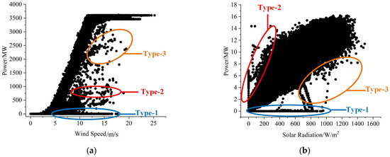
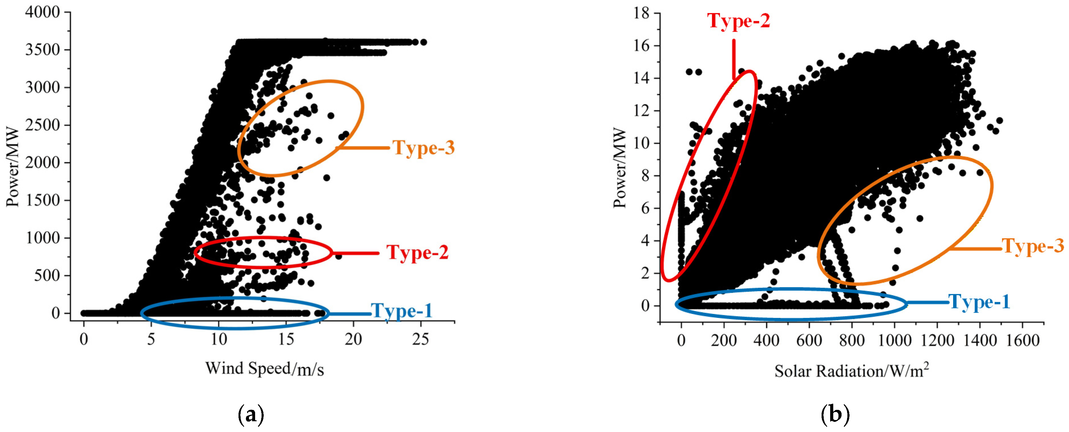
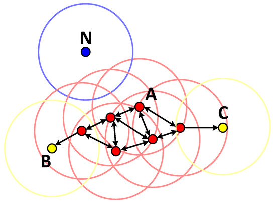
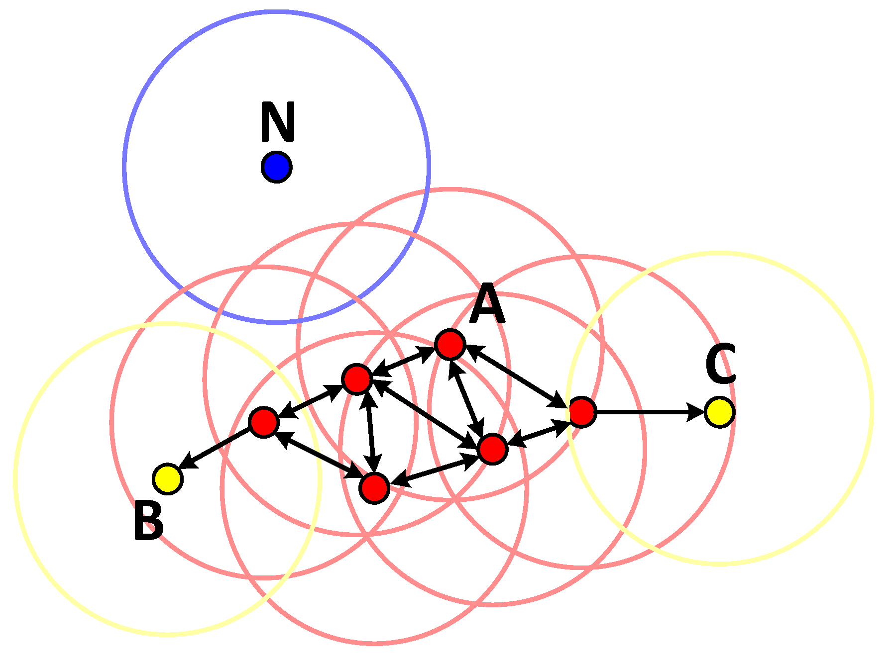
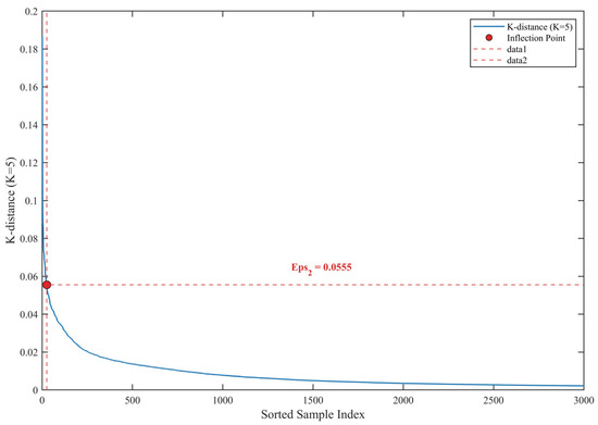
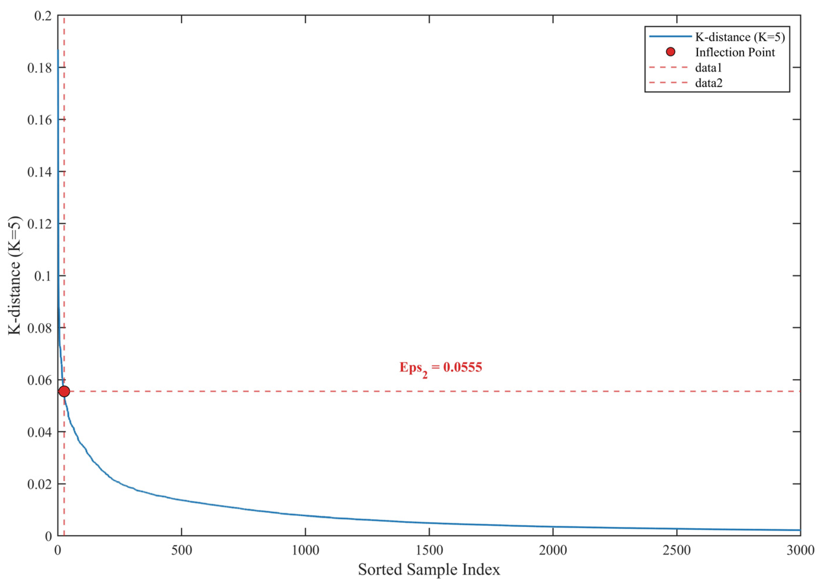
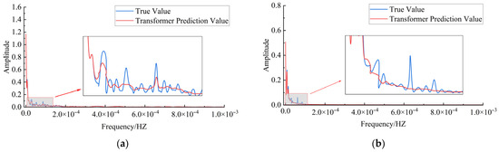
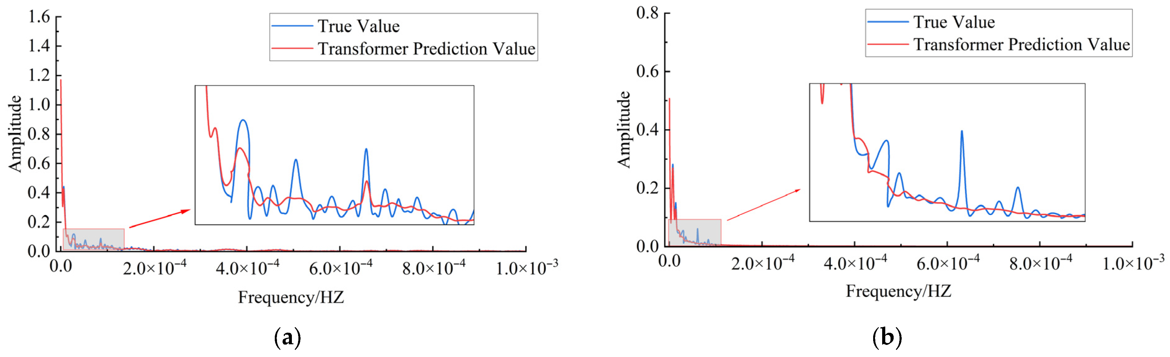
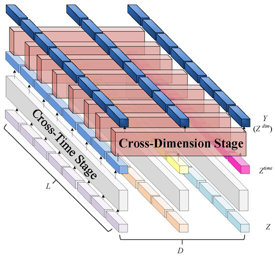
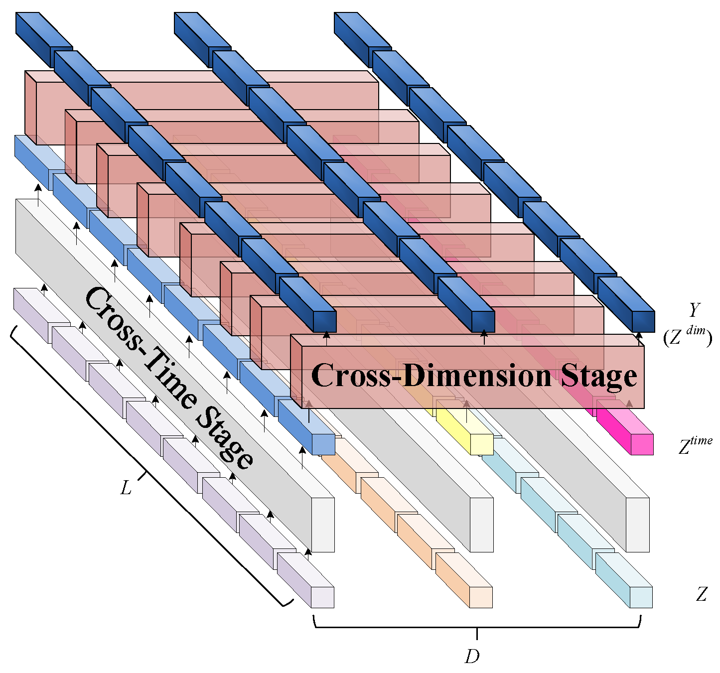
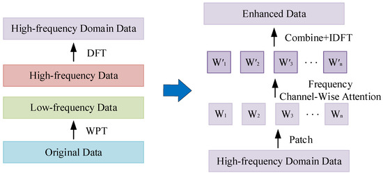
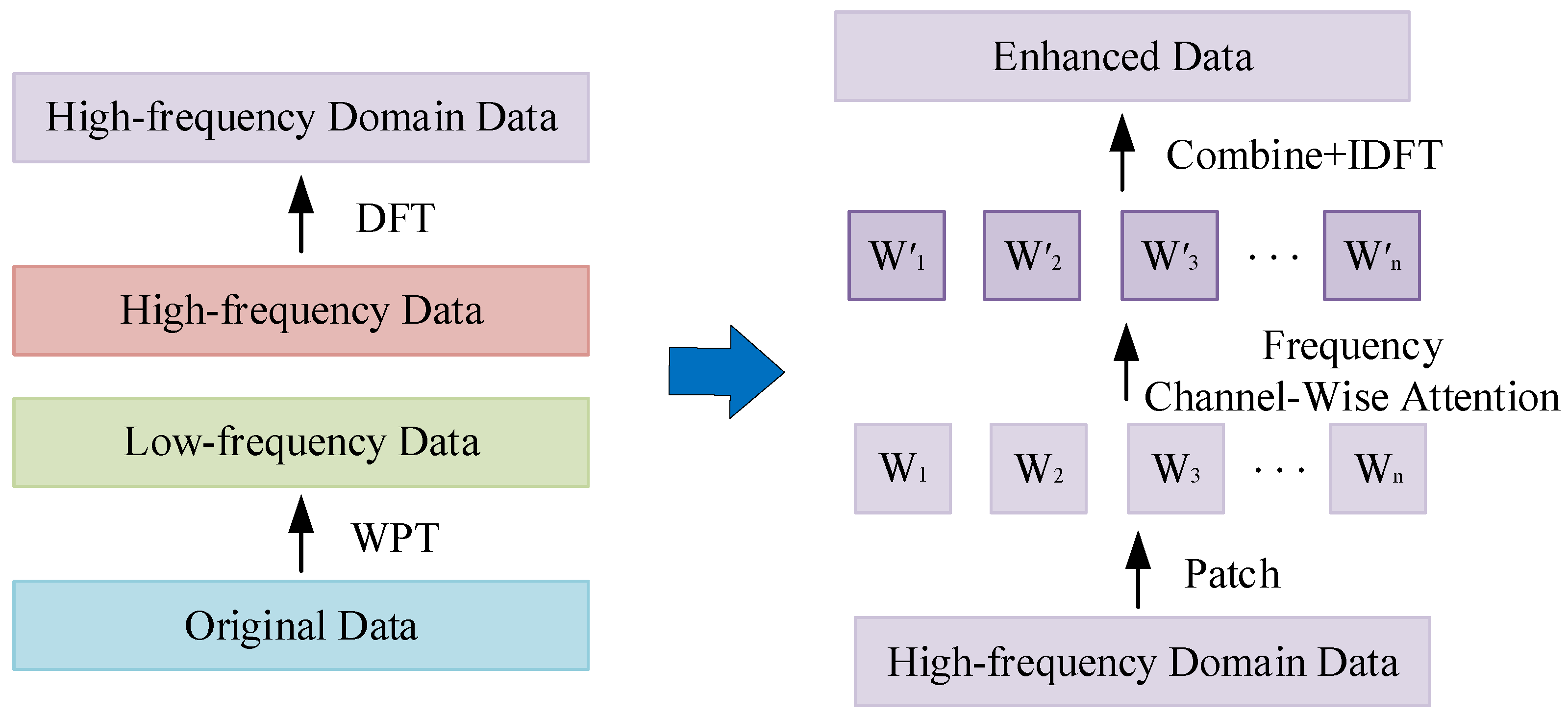
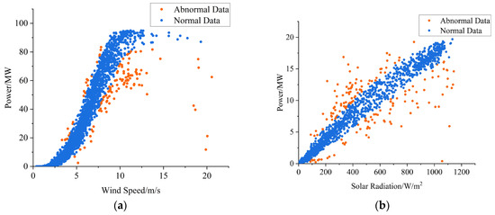
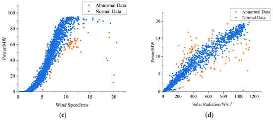
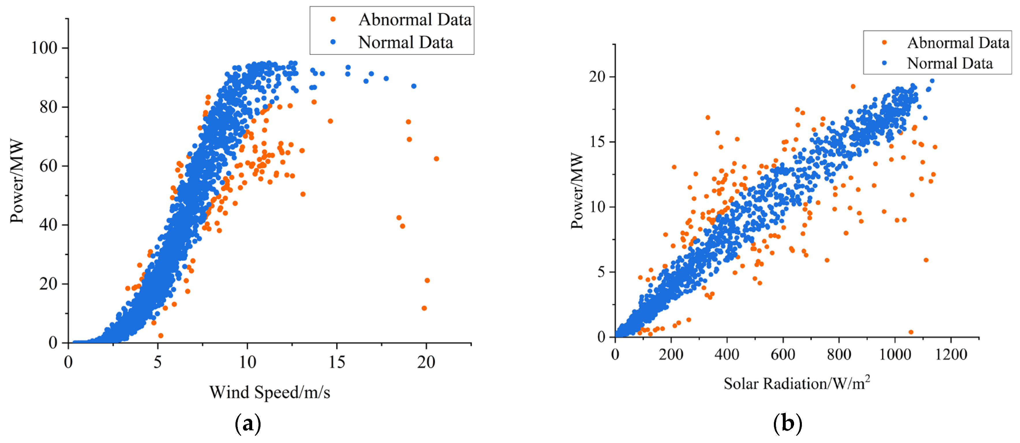
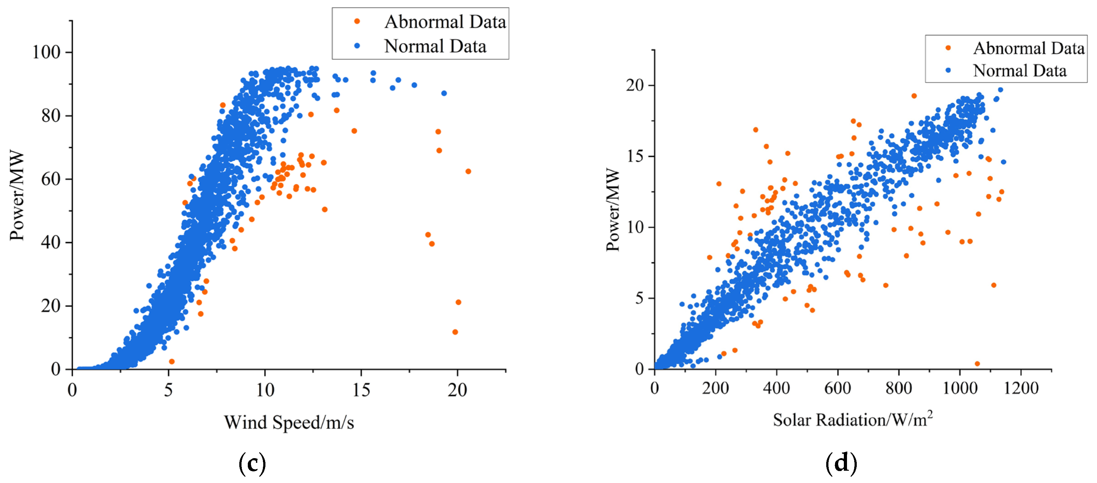
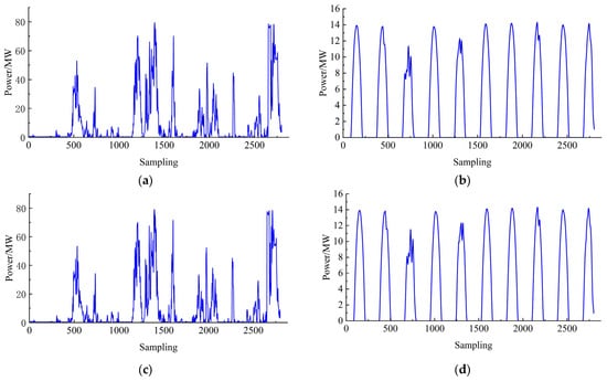
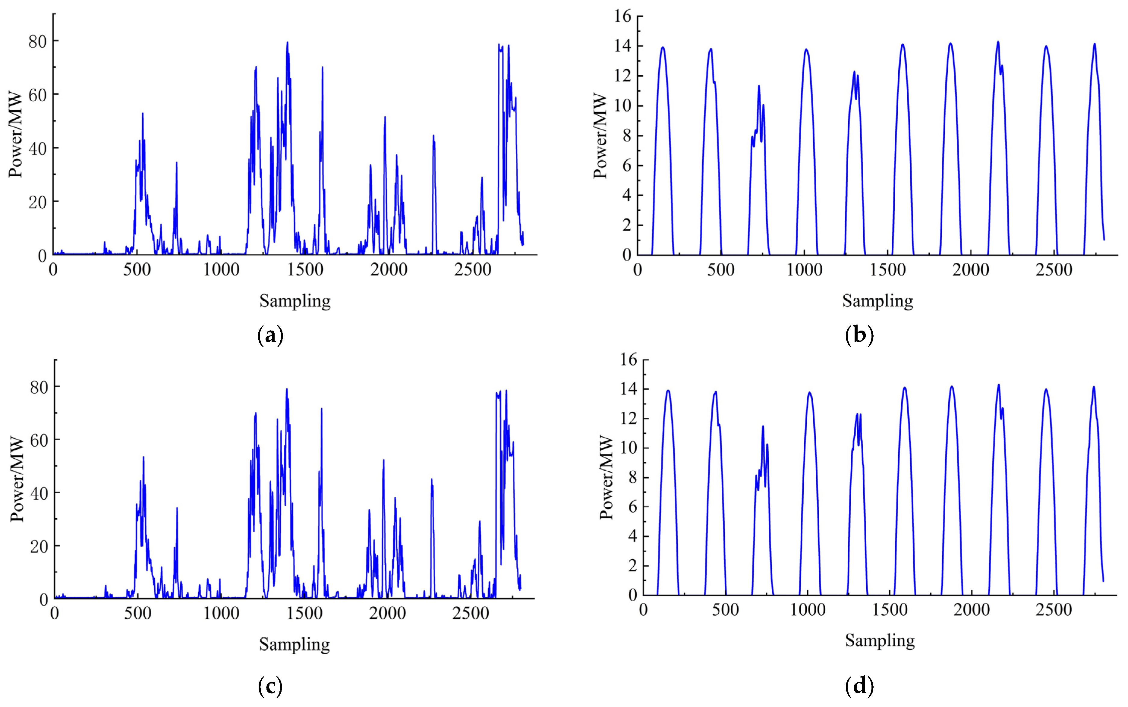
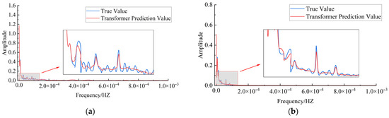
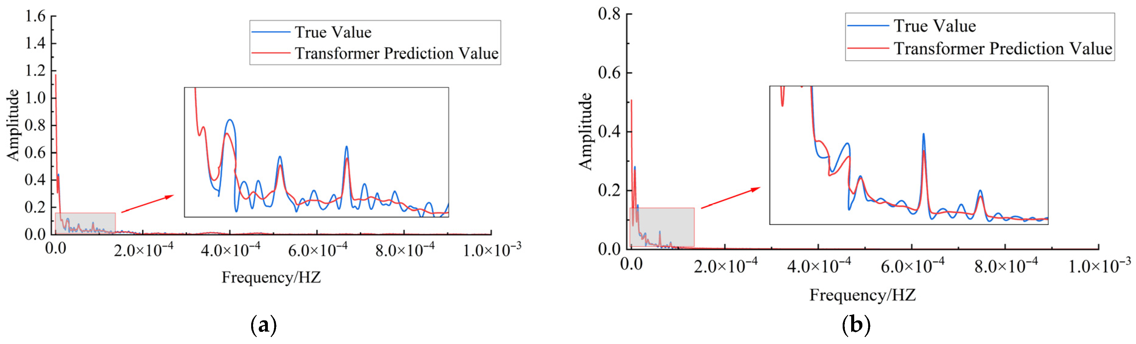
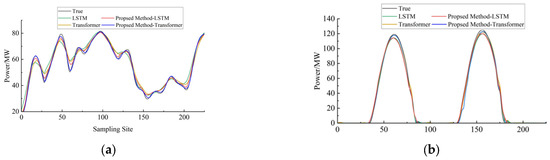
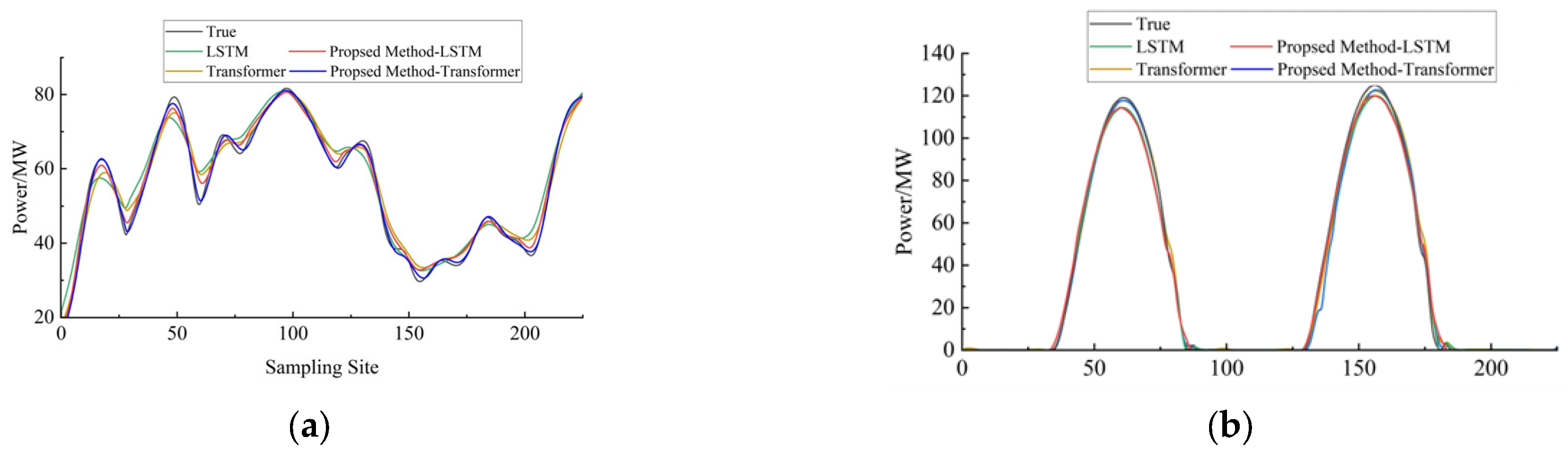
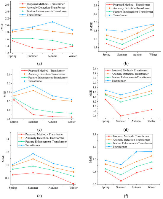
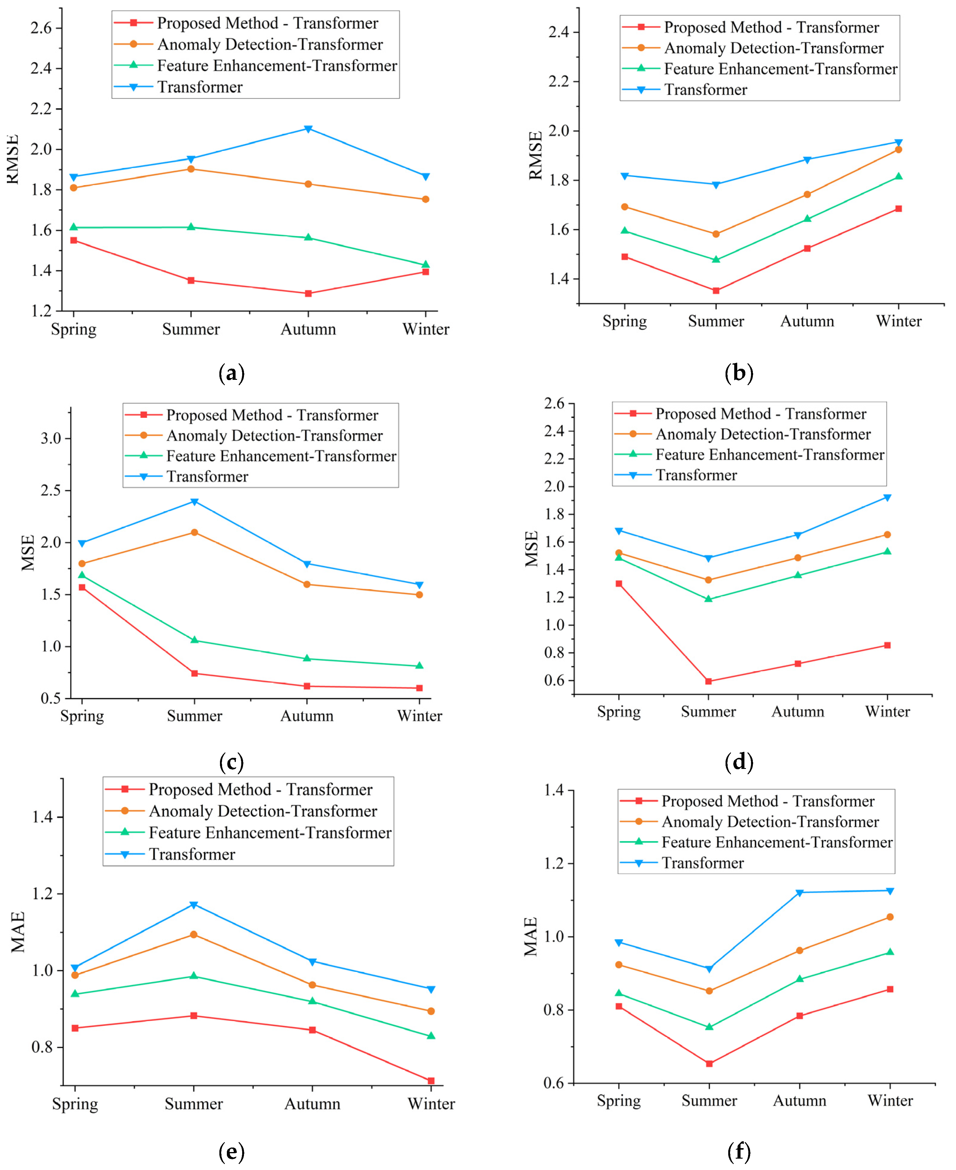

Disclaimer/Publisher’s Note: The statements, opinions and data contained in all publications are solely those of the individual author(s) and contributor(s) and not of MDPI and/or the editor(s). MDPI and/or the editor(s) disclaim responsibility for any injury to people or property resulting from any ideas, methods, instructions or products referred to in the content. |
© 2026 by the authors. Licensee MDPI, Basel, Switzerland. This article is an open access article distributed under the terms and conditions of the Creative Commons Attribution (CC BY) license.