Evidential Deep Learning for Quantification of Uncertainty in Lithium-Ion Batteries Remaining Useful Life Estimation

Abstract

Lithium-ion batteries are widely used across diverse applications due to their high energy density, long cycle life, and fast charging capabilities. As battery-powered systems become increasingly critical, accurate estimation of the Remaining Useful Life (RUL) is essential for ensuring reliability, safety, and effective maintenance planning. This work investigates Evidential Deep Learning (EDL) for data-driven RUL estimation and introduces a novel risk-aware loss function designed to enhance both predictive accuracy and uncertainty quantification in the End-of-Life (EoL) region, where precise and trustworthy predictions are most needed. Using a publicly available dataset of lithium iron phosphate (LFP) cells, we benchmark the proposed approach against a baseline Conv–LSTM model, Monte Carlo (MC) Dropout, and Deep Ensembles. The results show that integrating the risk-aware loss into the EDL framework substantially improves the calibration of predictive uncertainty while achieving state-of-the-art accuracy near EoL. Unlike MC Dropout and Deep Ensembles, which exhibit increasing or unstable uncertainty as degradation accelerates, the proposed EDL model demonstrates a consistent reduction in uncertainty and significantly higher reliability in late-stage predictions. The findings indicate that the risk-aware evidential framework offers a reliable and computationally efficient solution for battery RUL estimation, enabling more informed decision-making in both safety-critical and consumer-oriented applications.

1. Introduction

Lithium-ion batteries have become indispensable in both industrial applications and everyday life, powering devices ranging from smartphones and electric vehicles to industrial machinery and critical infrastructure systems. Their widespread adoption stems from their favorable characteristics, including high energy density, fast charging capabilities, and low self-discharge rates [1]. As the demand for battery-powered systems continues to grow, ensuring efficient and reliable battery management becomes increasingly critical to maintain safety, performance, and cost-effectiveness [2,3,4].

A central aspect of battery health monitoring is the estimation of the Remaining Useful Life (RUL), defined as the number of charge–discharge cycles a battery can undergo before reaching its End of Life (EoL) [5]. Accurate RUL prediction enables timely maintenance actions or battery replacement, reducing the risk of unexpected failures and improving system reliability. Failure to properly manage battery degradation can lead to severe consequences, including safety hazards such as thermal runaway, fire, and explosions, as documented in real-world incidents [6,7].

With the emergence of Industry 4.0 and the transition toward Industry 5.0, emphasizing human-centric automation, resilience, and sustainability, the role of Artificial Intelligence (AI) and machine learning (ML) in battery health management has grown substantially [8,9]. These methods are increasingly used to model battery degradation and predict future behavior. However, in safety-critical and user-facing applications, high predictive accuracy alone is insufficient. Standard regression models provide deterministic point estimates, failing to convey the confidence associated with their predictions. Consequently, equipping prognostic models with uncertainty quantification (UQ) capabilities is essential for fostering trust and enabling risk-aware decision-making.

The field of UQ in deep learning has evolved to address two distinct types of uncertainty: aleatoric, which arises from inherent data noise and sensor stochasticity, and epistemic, which reflects the model’s lack of knowledge in unseen or out-of-distribution regimes [10].

Early efforts to capture these uncertainties relied on Bayesian neural networks (BNNs) [11], which place probability distributions over network weights. While theoretically rigorous, BNNs are often computationally intractable for real-time battery management systems (BMSs) due to convergence difficulties and high sampling costs. To overcome this, approximate Bayesian methods have been widely adopted. Monte Carlo (MC) Dropout [12] estimates uncertainty by performing stochastic forward passes during inference. While effective, MC Dropout can be inconsistent in regression tasks and introduces latency due to the requirement of multiple inferences for a single prediction.

Currently, Deep Ensembles [13], aggregating predictions from multiple independently trained models, are considered the state-of-the-art for predictive uncertainty, offering superior calibration and robustness compared to BNNs and MC Dropout. However, the requirement to maintain, store, and execute multiple models simultaneously imposes a computational and memory burden that is often prohibitive for embedded hardware with strict resource constraints.

Contribution

In this work, we investigate Evidential Deep Learning (EDL) [14] as a superior alternative for battery prognostics. Unlike sampling-based methods (MC Dropout, Ensembles), EDL learns a higher-order probability distribution over the target parameters in a single forward pass, offering both computational efficiency and explicit uncertainty decomposition.

However, standard evidential regression losses treat all prediction errors equally. In the context of battery prognostics, the cost of misprediction is asymmetric: an error near the End-of-Life (EoL) carries significantly higher safety risks than an error in the early stages of life. To address this, we introduce a novel Risk-Aware Evidential Loss, which dynamically re-weights the evidence regularization based on the proximity to EoL. This forces the model to maintain conservative, well-calibrated uncertainty estimates in the safety-critical region.

The main contributions of this study are as follows:

• A Comprehensive UQ Framework: We propose a hybrid Convolutional-LSTM architecture integrated with an evidential output head, capable of quantifying both aleatoric and epistemic uncertainty in real-time without sampling.
• Risk-Aware Optimization: We introduce a modified loss function that embeds an exponential penalty for errors near the End-of-Life. We demonstrate that this modification resolves the issue of “increasing uncertainty” often seen in MC Dropout, leading to tighter and more reliable bounds near failure.
• Rigorous Benchmarking: We compare the proposed framework against two strong baselines: MC Dropout and Deep Ensembles. The evaluation goes beyond simple error metrics to include probabilistic calibration metrics and inference latency analysis.
• Efficiency Validation: We demonstrate that the proposed method matches the predictive accuracy of Deep Ensembles in the critical final cycles while reducing inference time by an order of magnitude, validating its suitability for embedded deployment.

2. Problem Description

The SoH of a battery is a key indicator of its long-term performance and operational condition relative to its initial capacity. It is commonly expressed as

$$So{H}_k={\displaystyle \frac{C_k}{C}}\times 100$$

where $C_k$ represents the battery capacity at cycle k and C is the nominal capacity. SoH provides a quantitative assessment of battery degradation and is influenced by various factors, including internal resistance, aging, temperature fluctuations, charge/discharge rates, and depth of discharge [15].

The RUL refers to the number of operational cycles left before a battery reaches the end of its serviceable life (EoL). It is formally defined at cycle k as

$${\mathrm{RUL}}_k=cycl{e}_{EoL}-k$$

where $cycl{e}_{EoL}$ denotes the End-of-Life cycle. For lithium-ion batteries, the EoL threshold is typically set when SoH drops below 80%, though lighter thresholds such as 70% may be applied in less safety-critical applications.

RUL estimation aims to predict how many cycles remain before a battery must be replaced. This task generally relies on commonly available battery measurements, such as capacity and temperature. Accurate RUL predictions are vital for preventing system failures, optimizing maintenance schedules, and extending the operational life of equipment. They are especially important in domains like aerospace, automotive, medical devices, and energy systems, where lithium-ion batteries are widely adopted.

Battery degradation is a complex, non-linear process affected by coupled electrochemical and thermal dynamics. Consequently, precise RUL estimation has emerged as a crucial challenge in predictive maintenance and battery health management.

2.1. RUL Estimation Approaches

RUL estimation methods can broadly be categorized into three classes: model-based, data-driven, and hybrid approaches.

Model-based methods rely on physical, chemical, or empirical models that describe battery degradation mechanisms. These include:

• Electrochemical models, which simulate internal reactions;
• Equivalent Circuit Models (ECMs), which replicate battery behavior using circuit components;
• Empirical models, which use simplified equations derived from observed data.

These approaches benefit from strong physical interpretability and reliability in data-scarce environments. However, their effectiveness may be limited by the need for extensive expert knowledge and assumptions that may not generalize across different battery types or usage scenarios [16,17,18].

Data-driven methods have gained popularity due to the rise of machine learning and the availability of large-scale datasets. These methods learn complex degradation patterns directly from data, without requiring explicitly physical models. Given the non-linear nature of battery aging, data-driven approaches, particularly deep learning models, are well suited to capturing intricate dependencies among features.

According to the taxonomy proposed in [19], data-driven approaches can be grouped into five main categories: neural network-based methods, generative models, kernel-based learning, probabilistic models, and fuzzy logic-based approaches.

Hybrid methods aim to combine the strengths of both model-based and data-driven approaches. These may involve fusing physical models with machine learning algorithms to enhance generalization and adaptivity. For instance, [20] demonstrates a hybrid system combining empirical models with Support Vector Regression (SVR) to simultaneously model degradation and quantify uncertainty.

2.2. Formalization of Uncertainty

In the context of deep learning for prognostics, predictive uncertainty is formally decomposed into two distinct components, each arising from fundamentally different sources:

1. Aleatoric Uncertainty (${\sigma }_a^2$): Also known as statistical or data uncertainty, this arises from the inherent noise and stochasticity in the data generation process (e.g., sensor noise, irreversible electrochemical variations). It is irreducible, meaning it cannot be removed by collecting more training data. For a heteroscedastic model, the data likelihood is modeled as a Gaussian:

$$p\left(y\right|\mathbf{x},\theta )=\mathcal{N}\left(y\right|f_{\theta }\left(\mathbf{x}\right),{\sigma }_a^2\left(\mathbf{x}\right))$$

(1)

2. Epistemic Uncertainty (${\sigma }_e^2$): Also known as model uncertainty, this arises from the lack of knowledge about the true model parameters $\theta$ or the model structure. It captures the uncertainty in regions of the input space where training data is sparse (out-of-distribution). Unlike aleatoric uncertainty, epistemic uncertainty is reducible; as the size of the training set $N\to \infty$, ${\sigma }_e^2\to 0$. In Bayesian terms, this is represented by the posterior distribution of the weights $p\left(\theta \right|\mathcal{D})$.

2.2.1. Monte Carlo Dropout

MC Dropout [12,21] provides a scalable approximation to BNNs. It interprets the dropout regularization technique, commonly used during training to prevent overfitting, as a variational Bayesian approximation of the posterior distribution.

During inference, rather than disabling dropout to obtain a single deterministic prediction, dropout is kept active. The model performs T stochastic forward passes for the same input $\mathbf{x}$, effectively sampling from the approximate posterior predictive distribution. For a regression task, the predictive mean ${\widehat{y}}_{MC}$ and the predictive variance ${\sigma }_{MC}^2$ are approximated as

$${\widehat{y}}_{MC}\approx {\displaystyle \frac{1}{T}}\sum _{t=1}^T{f}_{{\theta }_t}\left(\mathbf{x}\right)$$

(2)

$${\sigma }_{MC}^2\approx \underset{\mathrm{Epistemic}}{\underbrace{{\displaystyle \frac{1}{T}}\sum _{t=1}^T{(f_{{\theta }_t}\left(\mathbf{x}\right)-{\widehat{y}}_{MC})}^2}}+{\tau }^{-1}$$

(3)

where $f_{{\theta }_t}$ represents the network output with a random dropout mask applied and ${\tau }^{-1}$ represents the inverse model precision (often assumed constant or learned). While MC Dropout is easy to implement, it increases the inference computational cost by a factor of T (typically $T=50$ or 100) and introduces stochasticity into the prediction, which can be undesirable in deterministic control loops.

2.2.2. Deep Ensembles

The Deep Ensembles method [13,22] involves training M independent neural networks ${\left\{{\theta }_m\right\}}_{m=1}^M$ on the same dataset, using random initialization of parameters and random shuffling of data batches to induce diversity.

Unlike MC Dropout, which approximates a single mode of the posterior, Deep Ensembles can capture multiple modes, often resulting in better calibration. Each ensemble member outputs a mean ${\mu }_{{\theta }_m}\left(\mathbf{x}\right)$ and a variance ${\sigma }_{{\theta }_m}^2\left(\mathbf{x}\right)$. The final predictive distribution is a mixture of Gaussians, with the ensemble mean and total variance defined as

$${\widehat{y}}_{Ens}={\displaystyle \frac{1}{M}}\sum _{m=1}^M{\mu }_{{\theta }_m}\left(\mathbf{x}\right)$$

(4)

$${\sigma }_{Ens}^2=\underset{\mathrm{Aleatoric}}{\underbrace{{\displaystyle \frac{1}{M}}\sum _{m=1}^M{\sigma }_{{\theta }_m}^2\left(\mathbf{x}\right)}}+\underset{\mathrm{Epistemic}}{\underbrace{{\displaystyle \frac{1}{M}}\sum _{m=1}^M{({\mu }_{{\theta }_m}\left(\mathbf{x}\right)-{\widehat{y}}_{Ens})}^2}}$$

(5)

The first term averages the predicted data noise (aleatoric), while the second term captures the disagreement among models (epistemic). Although Deep Ensembles typically outperform MC Dropout in accuracy, they require maintaining M distinct models in memory and performing M forward passes, making them computationally expensive for resource-constrained battery management units.

2.2.3. Evidential Deep Learning

Standard BNNs approximate the posterior $p\left(\theta \right|\mathcal{D})$ via sampling (e.g., MC Dropout), which approximates the predictive variance as

$$\underset{\mathrm{Total}}{\underbrace{Var\left(y\right)}}\approx \underset{\mathrm{Aleatoric}}{\underbrace{{\displaystyle \frac{1}{T}}\sum _{t=1}^T{\sigma }_a^2\left({\mathbf{x}}_t\right)}}+\underset{\mathrm{Epistemic}}{\underbrace{{\displaystyle \frac{1}{T}}\sum _{t=1}^T{({\widehat{y}}_t-\overline{y})}^2}}$$

(6)

where T is the number of stochastic forward passes.

While effective, this sampling process introduces significant computational latency. In contrast, EDL [14] places a higher-order prior distribution directly over the likelihood parameters $(\mu ,{\sigma }^2)$. For regression, the target y is assumed to be drawn from a Gaussian distribution $\mathcal{N}(\mu ,{\sigma }^2)$, but the parameters $\mu$ and ${\sigma }^2$ are themselves drawn from a Normal–Inverse–Gamma (NIG) distribution:

$$\mu ,{\sigma }^2\sim \mathrm{NIG}(\gamma ,\nu ,\alpha ,\beta )$$

(7)

The neural network is trained to output the hyperparameters $\mathbf{m}=(\gamma ,\nu ,\alpha ,\beta )$ in a single deterministic forward pass. From these, the predictive mean and the decoupled uncertainties are derived analytically:

$$\begin{array}{cc}\hfill \mathbb{E}\left[y\right]& =\gamma \hfill \end{array}$$

(8)

$$\begin{array}{cc}\hfill \underset{\mathrm{Total}}{\underbrace{Var\left[y\right]}}& =\underset{\mathrm{Aleatoric}}{\underbrace{{\displaystyle \frac{\beta }{\alpha -1}}}}+\underset{\mathrm{Epistemic}}{\underbrace{{\displaystyle \frac{\beta }{\nu (\alpha -1)}}}}\hfill \end{array}$$

(9)

This formulation allows for efficient, real-time quantification of risk without the computational latency of sampling-based methods. The variable $\nu$ can be interpreted as the virtual evidence support, indicating how many training samples similar to the current input have been observed, while $\alpha$ and $\beta$ govern the shape and scale of the variance distribution. By leveraging this framework, the proposed model can explicity flag low-evidence predictions (high epistemic uncertainty) which is critical for identifying potential failure modes in battery operation.

3. Dataset

The dataset used in this study is provided by Toyota and the Massachusetts Institute of Technology (MIT) [23]. It includes cycling data from 124 commercial lithium iron phosphate (LFP)/graphite lithium-ion cells (model APR18650M1A), manufactured by A123 Systems (Hangzhou, China) and tested under fast-charging conditions until failure.

All batteries were operated in a controlled environment with a constant temperature of 30 °C. Voltage cut-offs for the charge/discharge cycles were fixed at 2.0 V (minimum) and 3.6 V (maximum). To generate a wide variety of charge curves and aging behaviors, different charging protocols were applied across cells. As a result, despite all the batteries having the same nominal capacity of 1.1 Ah, their lifespans varied significantly, ranging from 150 to 2200 cycles, reflecting the strong non-linear nature of battery degradation.

The charging process consisted of two constant current (CC) steps with a transition based on the State of Charge (SoC), followed by a constant current–constant voltage (CC-CV) phase at 1 A, beginning at approximately 80% SoC. The discharge process was standardized across all cells, using a constant current of 4 A.

The dataset is organized into three batches, each with minor procedural differences. For every battery, measurements are recorded both during cycling and at the end of each charge–discharge cycle, providing a comprehensive view of performance and degradation over time.

4. Methodology

The methodology proposed in this work integrates advanced signal processing, deep learning, and evidential reasoning to achieve robust Remaining Useful Life (RUL) estimation. The framework is designed to address two primary objectives: the accurate prediction of battery degradation, particularly near the critical End-of-Life (EoL) stage, and the reliable quantification of predictive uncertainty.

The workflow is structured into four sequential stages: (1) feature extraction and preprocessing, (2) neural network architecture design, (3) uncertainty quantification via Evidential Deep Learning (EDL), and (4) loss function formulation and training protocol.

4.1. Feature Engineering and Preprocessing

4.1.1. Feature Definition

To ensure adaptability and ease of replication, we selected features that are readily available in most public battery datasets. This approach minimizes the need for additional sensor instrumentation or preprocessing, ultimately reducing data acquisition costs and enhancing the generalization potential of our method for future deployments.

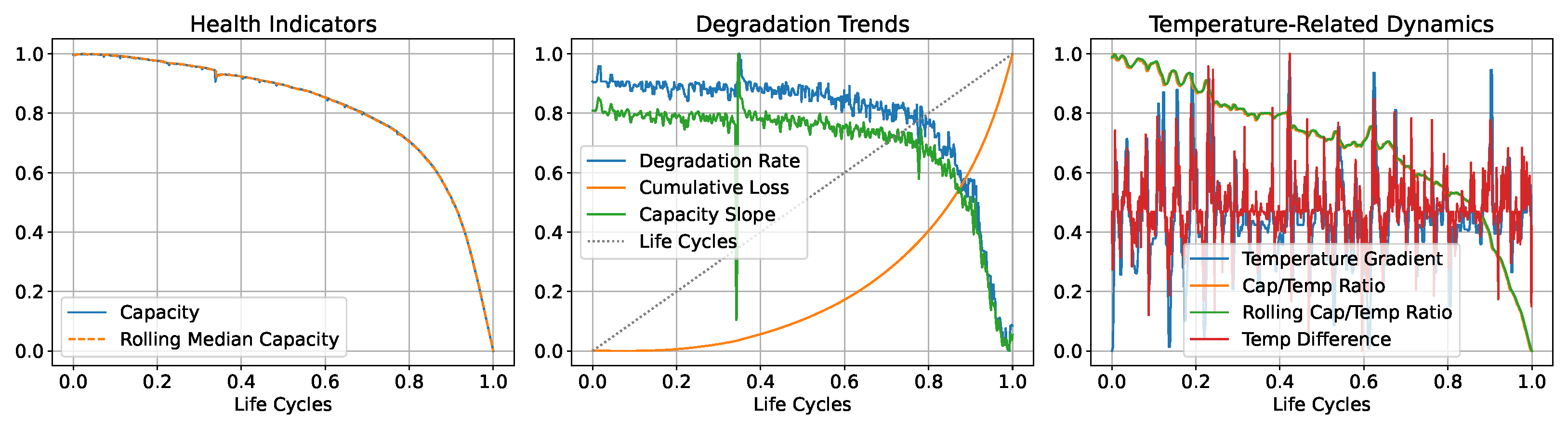
A total of 10 features, which can be seen in Figure 1, were selected to describe the battery state at each operational cycle. These features are derived primarily from capacity and temperature measurements, which are commonly available. We categorize them into three functional groups: (i) health indicators, (ii) degradation trends, and (iii) temperature-related dynamics.

1. Health Indicators: The core indicator of battery status is the SoH, defined as the ratio between the capacity $C_i$ at the i-th cycle and the nominal capacity C:

$$So{H}_i={\displaystyle \frac{C_i}{C}}$$

To provide a smoothed representation, we also compute the rolling median of SoH, reducing the influence of outliers and sensor spikes:

$$So{H}_{me{d}_i}=median(So{H}_{i-w},\dots ,So{H}_i)$$

where w is the rolling window size.

2. Degradation Trends: We model degradation both at local and cumulative scales:

• The i-th SoH loss between consecutive cycles is

  $$So{H}_{los{s}_i}=So{H}_i-So{H}_{i-1}$$
• The cumulative SoH loss over time is obtained by summing all degradation values up to the current cycle:

  $$So{H}_{c-los{s}_i}=\sum _{j=1}^{i}So{H}_{los{s}_j}$$
• The SoH slope is computed by fitting a linear regression to all SoH values from the start of life (cycle 0) to the current cycle i, capturing the overall degradation trajectory:

  $$slop{e}_i=linear\text{\_}regression(So{H}_0,\dots ,So{H}_i)$$
• We also include a scalar cycle index to represent the current life cycle count:

  $$cycl{e}_i=i$$

3. Temperature-Related Dynamics: Thermal behavior plays a key role in battery degradation. Accordingly, we define several temperature-based features:

• The temperature gradient from the initial value $T_0$ to the current temperature $T_i$ is

  $$T_{gra{d}_i}={\displaystyle \frac{T_i-T_0}{i}}$$
• The temperature difference between two consecutive cycles is

  $$T_{dif{f}_i}=T_i-T_{i-1}$$
• The SoH-to-temperature ratio reflects the correlation between health and thermal conditions:

  $$rati{o}_i={\displaystyle \frac{C_i}{T_i}}$$
• As with SoH, we compute the rolling median of the SoH–temperature ratio for a more noise-resilient version:

  $$s\text{\_}rati{o}_i=median(rati{o}_{i-w},\dots ,rati{o}_i)$$

4.1.2. Data Cleaning and Normalization

Raw battery sensor data often contains high-frequency noise and transient spikes due to sensor inaccuracies or relaxation effects. To mitigate this, a rolling median filter with a kernel size of 5 was applied to the capacity and temperature features prior to normalization. This step ensures that the model learns from the underlying degradation trend rather than overfitting to sensor noise.

Following smoothing, all input features are normalized to the $[0,1]$ interval using min–max normalization to ensure uniform feature scaling:

$$d_n={\displaystyle \frac{d-d_{min}}{d_{max}-d_{min}}}$$

where $d_n$ is the normalized value and $d_{min}$ and $d_{max}$ represent the minimum and maximum values of each feature computed strictly over the training set to prevent information leakage.

4.2. Model Architecture

The proposed architecture is a hybrid Convolutional-LSTM network enhanced with an attention mechanism. While the foundational structure draws from [24], this work introduces an evidential regression head to quantify aleatoric and epistemic uncertainty simultaneously. The model processes a sliding window of historical sensor data $X\in {\mathbb{R}}^{W\times F}$, where $W=20$ is the window size and $F=10$ is the number of input features.

The architecture consists of four distinct functional blocks:

• Convolutional Feature Extractor: To efficiently process high-dimensional temporal input data and capture local degradation patterns, the input is first processed by a convolutional block. This block comprises two 1D convolutional layers with 32 and 64 filters, respectively. Both layers utilize a kernel size of 5, the ‘same’ padding to preserve temporal alignment, and Rectified Linear Unit (ReLU) activation. Each convolutional layer is followed by a Max Pooling operation (pool size 2) to downsample the feature map, effectively compressing the temporal dimension from 20 to 5 time steps while retaining spatially invariant degradation patterns.
• LSTM Encoder–Decoder: The compressed feature sequence is fed into a Long Short-Term Memory (LSTM) encoder with 128 units. This layer outputs the full sequence of hidden states ($H_{enc}$) and the final internal states ($h_T,c_T$). Batch normalization (momentum = 0.6) is applied to the final states to stabilize the transition to the decoder. A RepeatVector layer prepares the input for the decoder LSTM (128 units), which reconstructs the temporal dependencies using the encoder’s final state as initialization.
• Attention Mechanism: To allow the model to focus on specific historical degradation events, a dot-product attention mechanism is applied. The attention scores are computed between the decoder output and the encoder hidden states, followed by a ReLU activation to determine the attention weights. These weights are used to compute a context vector, which is concatenated with the decoder output. A dropout layer with a rate of 0.4 is applied to this combined representation to prevent overfitting.
• Evidential Output Head: The standard dense output layer is replaced by a DenseNormalGamma layer [25]. Unlike standard regression which outputs a scalar $\widehat{y}$, this layer projects the 256-dimensional feature vector (128 context + 128 decoder) into four evidential parameters $\mathbf{m}=(\gamma ,\nu ,\alpha ,\beta )$. These parameters define a Normal–Gamma distribution, enabling the simultaneous prediction of the RUL target, the aleatoric uncertainty (data noise), and the epistemic uncertainty (model confidence).

The detailed architectural parameters, output shapes, and layer-wise parameter counts are summarized in

Table 1. Detailed summary of the proposed EDL-RUL architecture parameters.

Functional Block	Layer Details	Output Shape	Params
Input	$W=20,F=10$	(None, 20, 10)	0
Convolutional Block	Conv1D (32 filters, $k=5$, ReLU)	(None, 20, 32)	1632
	MaxPool1D	(None, 10, 32)	0
	Conv1D (64 filters, $k=5$, ReLU)	(None, 10, 64)	10,304
	MaxPool1D	(None, 5, 64)	0
Encoder–Decoder	LSTM Encoder (128 units)	(None, 5, 128)	98,816
	Batch Normalization	(None, 128)	512
	LSTM Decoder (128 units)	(None, 1, 128)	131,584
Attention & Merge	Dot Product Attention	(None, 1, 128)	0
	Batch Normalization	(None, 1, 128)	512
	Concatenate	(None, 256)	0
	Dropout ($p=0.4$)	(None, 256)	0
Output	DenseNormalGamma	(None, 4)	1028
Total			244,900

.

4.3. Loss Function Formulation

To address the dual objective of precise RUL estimation near the EoL and reliable uncertainty quantification, we investigate a progression of loss functions. This study evaluates three distinct formulations: (1) a domain-specific baseline (${\mathcal{L}}_{ECF}$), (2) a standard uncertainty-aware baseline (${\mathcal{L}}_{EDL}$), and (3) our proposed Risk-Aware Evidential Loss (${\mathcal{L}}_{risk}$), which integrates the strengths of the former two. We also evaluate a linear combination of the baselines (${\mathcal{L}}_{hybrid}$) as an intermediate benchmark.

4.3.1. Foundational Loss Functions

Exponential Custom Function (${\mathcal{L}}_{ECF}$): Proposed in [24], this loss functions as a weighted Mean Squared Error (MSE). It introduces an exponential term $\Theta$ that amplifies the penalty for errors as the target RUL ($y_i$) approaches zero (EoL). This encourages the model to prioritize accuracy in the safety-critical degradation zone:

$${\mathcal{L}}_{ECF}={\displaystyle \frac{1}{N}}\sum _{i=1}^N{(y_i-{\widehat{y}}_i)}^2·\underset{\Theta }{\underbrace{(e^{\beta (1-y_i)}-1)}}$$

(10)

where $\beta$ is a tunable scaling factor. While ${\mathcal{L}}_{ECF}$ improves late-stage accuracy, it is a point-prediction loss and cannot quantify uncertainty.

Evidential Loss Function (${\mathcal{L}}_{EDL}$): To enable uncertainty quantification, we adopt the loss proposed in [25]. It consists of a negative log-likelihood term (${\mathcal{L}}_{NLL}$) to fit the Normal–Inverse–Gamma distribution and a regularization term (${\mathcal{L}}_R$) to penalize incorrect evidence (overconfidence):

$${\mathcal{L}}_{EDL}={\mathcal{L}}_{NLL}+\lambda {\mathcal{L}}_R$$

(11)

The regularization term is defined as

$${\mathcal{L}}_R=|y_i-\gamma |·(2\nu +\alpha )$$

(12)

where $\gamma$ is the predicted mean and $(2\nu +\alpha )$ represents the total evidence. While ${\mathcal{L}}_{EDL}$ successfully quantifies uncertainty, it applies a uniform penalty across the battery lifespan, failing to account for the increased risk associated with errors near EoL.

4.3.2. Intermediate Approach: Hybrid Loss (${\mathcal{L}}_{hybrid}$)

As a first step toward integrating EoL-awareness with uncertainty, we defined a combined loss function that linearly weights the two objectives:

$${\mathcal{L}}_{hybrid}=\omega ·{\mathcal{L}}_{ECF}+(1-\omega )·{\mathcal{L}}_{EDL}$$

(13)

where $\omega \in [0,1]$ balances the trade-off. While this approach improves performance, the objectives remain mathematically decoupled; the uncertainty estimation mechanism (${\mathcal{L}}_{EDL}$) is not explicitly informed by the proximity to failure (${\mathcal{L}}_{ECF}$).

4.3.3. Proposed Approach: Risk-Aware Evidential Loss (${\mathcal{L}}_{risk}$)

To overcome the limitations of the linear combination, we propose a novel Risk-Aware Evidential Loss. We embed the exponential weighting term $\Theta$ directly into the regularization component of the evidential loss. The formulation is as follows:

$${\mathcal{L}}_{risk}={\mathcal{L}}_{NLL}+\lambda {\mathcal{L}}_{reg}^R$$

(14)

$${\mathcal{L}}_{reg}^R=|y_i-\gamma |·(2\nu +\alpha )·\underset{\Theta }{\underbrace{(e^{\beta (1-y_i)}-1)}}$$

(15)

By multiplying the KL-divergence regularization term by $\Theta$, the model incurs a significantly higher penalty for expressing high confidence (high evidence $\nu ,\alpha$) if the prediction is incorrect near the End-of-Life.

Convergence Validity: Since the exponential term $\Theta$ is strictly positive and bounded for normalized inputs $y_i\in [0,1]$, the modified regularization term acts as a dynamic scaling of the original ${\mathcal{L}}_R$. This preserves the convexity properties required for convergence while reshaping the gradient landscape to create a risk-sensitive optimization surface.

4.4. Training Protocol

4.4.1. Dataset Partitioning

To evaluate the model’s generalization capability on unseen devices, the dataset was partitioned at the battery level rather than the cycle level. Splitting by cycle would introduce temporal leakage, as the model would train on adjacent cycles of the same battery used for testing.

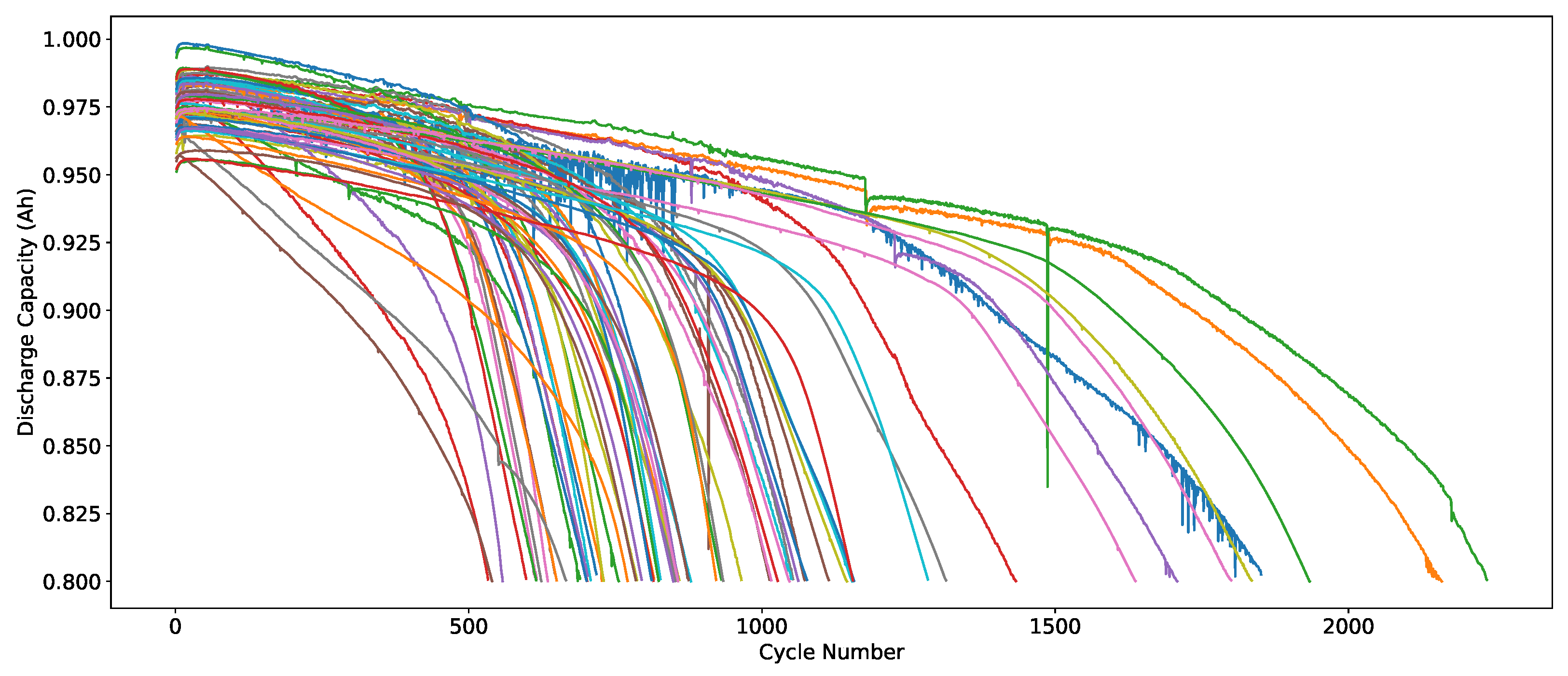
The 124 cells were divided into training (103 batteries) validation (13 batteries), and test (8 batteries) subsets. To ensure that the test set is representative of the entire population, the split was stratified across the three data batches provided by the source dataset [15], ensuring that different charging protocols and aging behaviors are equally represented in all subsets. The split ratio was chosen to ensure that all charging policies were represented in the training set while maintaining a sufficiently large hold-out portion (21 batteries) for validation and testing, which still contains thousands of unseen lifecycle measurements. In Figure 2 are shown all the degradation trends used in the training set.

4.4.2. Hyperparameter Tuning

A grid-search optimization was conducted to identify the optimal model configuration. The input sliding window size was a critical parameter; a window of size $w=20$ was selected as the optimal trade-off. This duration captures sufficient historical context to model the local degradation gradient ($\Delta SoH$) while minimizing the input latency required for the first prediction.

We also optimized the parameters governing the loss function, specifically the weighting factor $\omega$ (for ${\mathcal{L}}_{hybrid}$) and the exponential amplification factor $\beta$ (for ${\mathcal{L}}_{ECF}$ and ${\mathcal{L}}_{risk}$).

Table 2. Hyperparameter optimization results.

Hyperparameter	Range	Step	Best Value
Window size	(10, 60)	10	20
Filters (1st Conv layer)	(16, 64)	16	32
Filters (2nd Conv layer)	(32, 128)	32	64
Kernel size (Conv layers)	(2, 5)	1	5
Units in LSTM layers	(32, 128)	32	128
Dropout rate	(0.1, 0.5)	0.1	0.4
Loss Function Parameters
Exponential factor ($\beta$)	(1, 5)	1	3.0
Combined weight ($\omega$)	(0.0, 1.0)	0.1	0.8

details the hyperparameter search space and the final selected values.

4.5. Evaluation Metrics

To strictly assess both the regression performance and the quality of the uncertainty estimates, we employ a comprehensive set of metrics divided into two categories: prediction accuracy and uncertainty calibration.

4.5.1. Prediction Accuracy Metrics

Standard regression metrics are used to quantify the error between the predicted RUL and the ground truth.

• Mean Absolute Error (MAE): Measures the average magnitude of errors, providing a linear penalty for deviations.

  $$MAE={\displaystyle \frac{1}{N}}\sum _{i=1}^N|y_i-{\widehat{y}}_i|$$

  (16)
• Root Mean Squared Error (RMSE): Penalizes larger errors more heavily, making it sensitive to outliers and critical failures.

  $$RMSE=\sqrt{{\displaystyle \frac{1}{N}}\sum _{i=1}^N{(y_i-{\widehat{y}}_i)}^2}$$

  (17)

  where $y_i$ is the actual RUL, ${\widehat{y}}_i$ is the predicted mean RUL, and N is the total number of test samples.

4.5.2. Uncertainty Quantification Metrics

Evaluating a probabilistic model requires assessing whether its confidence intervals are trustworthy (calibration) and useful (sharpness). For all metrics, we assume a 95% confidence interval defined by lower bound $L_i={\widehat{y}}_i-1.96{\sigma }_i$ and upper bound $U_i={\widehat{y}}_i+1.96{\sigma }_i$, where ${\sigma }_i$ is the predicted total uncertainty.

• Prediction Interval Coverage Probability (PICP): Measures the reliability of the model’s uncertainty. It represents the percentage of ground truth values that fall within the predicted 95% confidence interval. Ideally, $\mathrm{PICP}\approx 0.95$.

  $$PICP={\displaystyle \frac{1}{N}}\sum _{i=1}^N\mathbf{1}(L_i\le y_i\le U_i)$$

  (18)

  where $\mathbf{1}(·)$ is the indicator function.
• Mean Prediction Interval Width (MPIW): Measures the sharpness of the uncertainty. A lower MPIW indicates a more precise model, provided that the PICP constraint (coverage) is satisfied.

  $$MPIW={\displaystyle \frac{1}{N}}\sum _{i=1}^N(U_i-L_i)$$

  (19)
• Negative Log-Likelihood (NLL): A proper scoring rule that evaluates the overall quality of the probabilistic fit. It simultaneously rewards accurate mean predictions and calibrated variance estimates while penalizing overconfidence on erroneous predictions.

  $$NLL={\displaystyle \frac{1}{N}}\sum _{i=1}^N\left({\displaystyle \frac{ln\left(2\pi {\sigma }_i^2\right)}{2}}+{\displaystyle \frac{{(y_i-{\widehat{y}}_i)}^2}{2{\sigma }_i^2}}\right)$$

  (20)

5. Results

The performance of the proposed EDL framework was evaluated against two probabilistic baselines: MC Dropout and Deep Ensembles. The evaluation focuses on three key dimensions: predictive accuracy (MAE, RMSE), probabilistic calibration (PICP, MPIW, NLL), and deployment feasibility (inference time).

5.1. Overall Predictive and Probabilistic Performance

Table 3. Overall performance comparison across methods. Best results are in bold.

Method	MAE	RMSE	PICP ↑	MPIW ↓	NLL ↓
Baseline	29.58	43.36	–	–	–
MC Dropout	39.94	50.47	0.665	0.119	2.242
Deep Ensemble	33.54	49.06	0.733	0.112	−0.500
EDL	28.08	18.79	0.988	0.254	−1.794
${\mathrm{EDL}}_{{\mathcal{L}}_{\mathrm{hybrid}}}$	22.98	31.72	0.995	0.272	−1.783
${\mathrm{EDL}}_{{\mathcal{L}}_{\mathrm{risk}}}$	25.69	35.30	0.992	0.237	−1.826

summarizes the global performance of each method. Among the baselines, the Deep Ensemble method exhibits the best point-wise accuracy, achieving an MAE of 33.54, but its probabilistic calibration is noticeably poor, as reflected by a PICP of 0.733. This implies that its 95% prediction intervals exclude the true RUL values in more than one quarter of cases. A similar calibration issue appears for the MC Dropout method, whose PICP of 0.665 demonstrates clear under-coverage.

The proposed EDL-based models display markedly stronger uncertainty calibration. The proposed ${\mathrm{EDL}}_{{\mathcal{L}}_{\mathrm{risk}}}$ achieves a PICP of 0.992 and the lowest NLL value of $-1.826$, implying a more faithful alignment between the predicted evidential distributions and the degradation dynamics. Although its MPIW of 0.237 is wider than the Deep Ensemble’s 0.112, this wider interval is justified by the significant gain in calibration, particularly for a safety-critical domain. The hybrid variant, ${\mathrm{EDL}}_{{\mathcal{L}}_{\mathrm{hybrid}}}$, obtains the strongest point-wise accuracy overall with an MAE of 22.98 and a PICP of 0.995, indicating that integrating the hybrid objective yields both precise and well-calibrated predictions.

5.2. Inference Efficiency

Table 4. Inference time comparison for uncertainty-aware methods. Best results are in bold.

Method	Inference Time (s) ↓
Baseline	0.43
MC Dropout	4.970
Deep Ensemble	4.455
EDL	0.456
${\mathrm{EDL}}_{{\mathcal{L}}_{\mathrm{hybrid}}}$	0.415
${\mathrm{EDL}}_{{\mathcal{L}}_{\mathrm{risk}}}$	0.442

evaluates the inference time to emphasize computational efficiency in embedded BMS settings. The MC Dropout and Deep Ensemble methods require multiple forward passes per prediction, resulting in inference times of 4.970 s and 4.455 s, respectively. In contrast, the EDL approach requires only a single forward pass. ${\mathrm{EDL}}_{{\mathcal{L}}_{\mathrm{hybrid}}}$ achieves the fastest execution at 0.415 s, closely followed by ${\mathrm{EDL}}_{{\mathcal{L}}_{\mathrm{risk}}}$ at 0.442 s. This represents roughly a tenfold improvement in computational efficiency relative to the ensemble-based baselines, enabling real-time deployment in resource-constrained environments.

5.3. Cycle-Wise Accuracy Across Battery Degradation Phases

The cycle-dependent MAE results in

Table 5. Cycle-wise MAE performance breakdown. Best results are in bold.

Method	Full	Last 400	Last 200	Last 100	Last 50
Baseline	29.58	14.72	7.50	3.95	2.21
MC Dropout	34.94	16.10	8.35	4.84	3.66
Deep Ensemble	30.42	12.48	7.80	4.68	3.90
EDL	28.08	18.79	10.40	4.83	4.03
${\mathrm{EDL}}_{{\mathcal{L}}_{\mathrm{hybrid}}}$	22.98	15.84	8.92	5.19	1.82
${\mathrm{EDL}}_{{\mathcal{L}}_{\mathrm{risk}}}$	25.69	15.57	8.22	3.66	1.79

reveal a distinct performance crossover between ensemble-based and evidential models. During early and mid-life degradation phases, the Deep Ensemble achieves the lowest MAE, with values of 12.48 in the last 400 cycles and 7.80 in the last 200 cycles. This behavior is expected, as ensemble averaging effectively compensates for noise during slowly varying degradation regimes.

However, EDL-based methods become superior as the battery approaches EoL. ${\mathrm{EDL}}_{{\mathcal{L}}_{\mathrm{risk}}}$ achieves an MAE of 3.66 in the last 100 cycles and 1.79 in the last 50 cycles, outperforming all other models and improving substantially over the Deep Ensemble’s 4.68 and 3.90 in the same regions. These improvements underscore the ability of the risk-sensitive loss to emphasize accurate predictions in critical, rapidly changing degradation intervals.

The RMSE trends reported in

Table 6. Cycle-wise RMSE performance breakdown. Best results are in bold.

Method	Full	Last 400	Last 200	Last 100	Last 50
Baseline	43.36	19.61	9.60	4.86	2.62
MC Dropout	50.47	21.15	10.31	5.63	4.16
Deep Ensemble	49.06	17.16	9.98	5.46	4.52
EDL	38.89	24.18	13.28	5.90	4.68
${\mathrm{EDL}}_{{\mathcal{L}}_{\mathrm{hybrid}}}$	31.72	20.78	10.93	6.84	2.19
${\mathrm{EDL}}_{{\mathcal{L}}_{\mathrm{risk}}}$	35.30	24.15	10.96	4.78	2.14

reinforce this behavior. Although the Deep Ensemble yields the smallest RMSE in the last 400 cycles (17.16) and the last 200 cycles (9.98), ${\mathrm{EDL}}_{{\mathcal{L}}_{\mathrm{risk}}}$ achieves the lowest RMSE values of 4.78 and 2.14 in the last 100 and 50 cycles, respectively. This indicates that evidential models better capture the non-linear acceleration of degradation, maintaining robustness when failure becomes imminent.

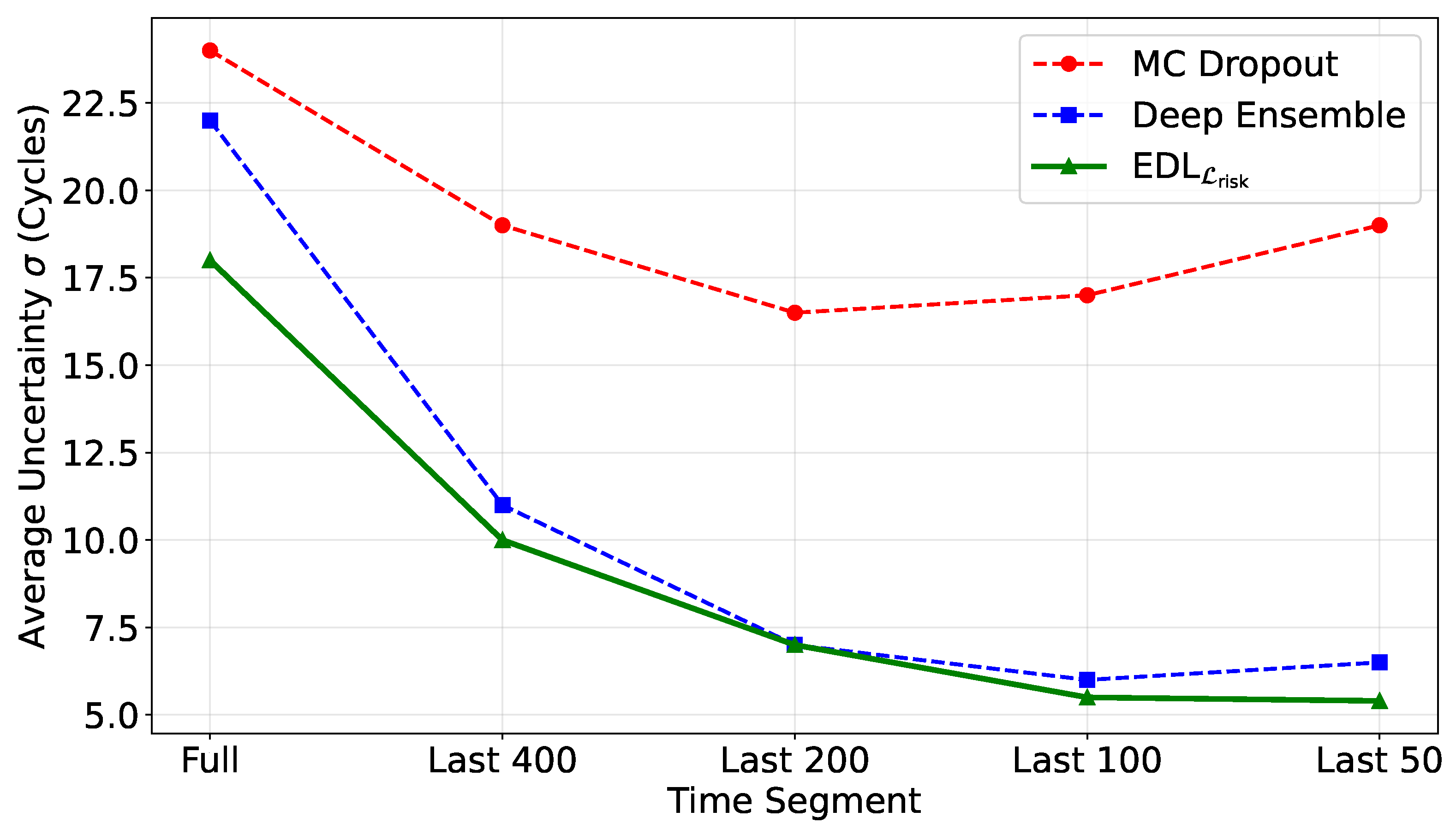
A key distinction between the methods is the trend of uncertainty as the battery degrades. As shown in Figure 3, the uncertainty ($\sigma$) for MC Dropout and Deep Ensembles tends to remain high or increase near the EoL. In contrast, the ${\mathrm{EDL}}_{{\mathcal{L}}_{\mathrm{risk}}}$ approach exhibits a Confidence Convergence property, where the predicted uncertainty steadily decreases as the system approaches failure.

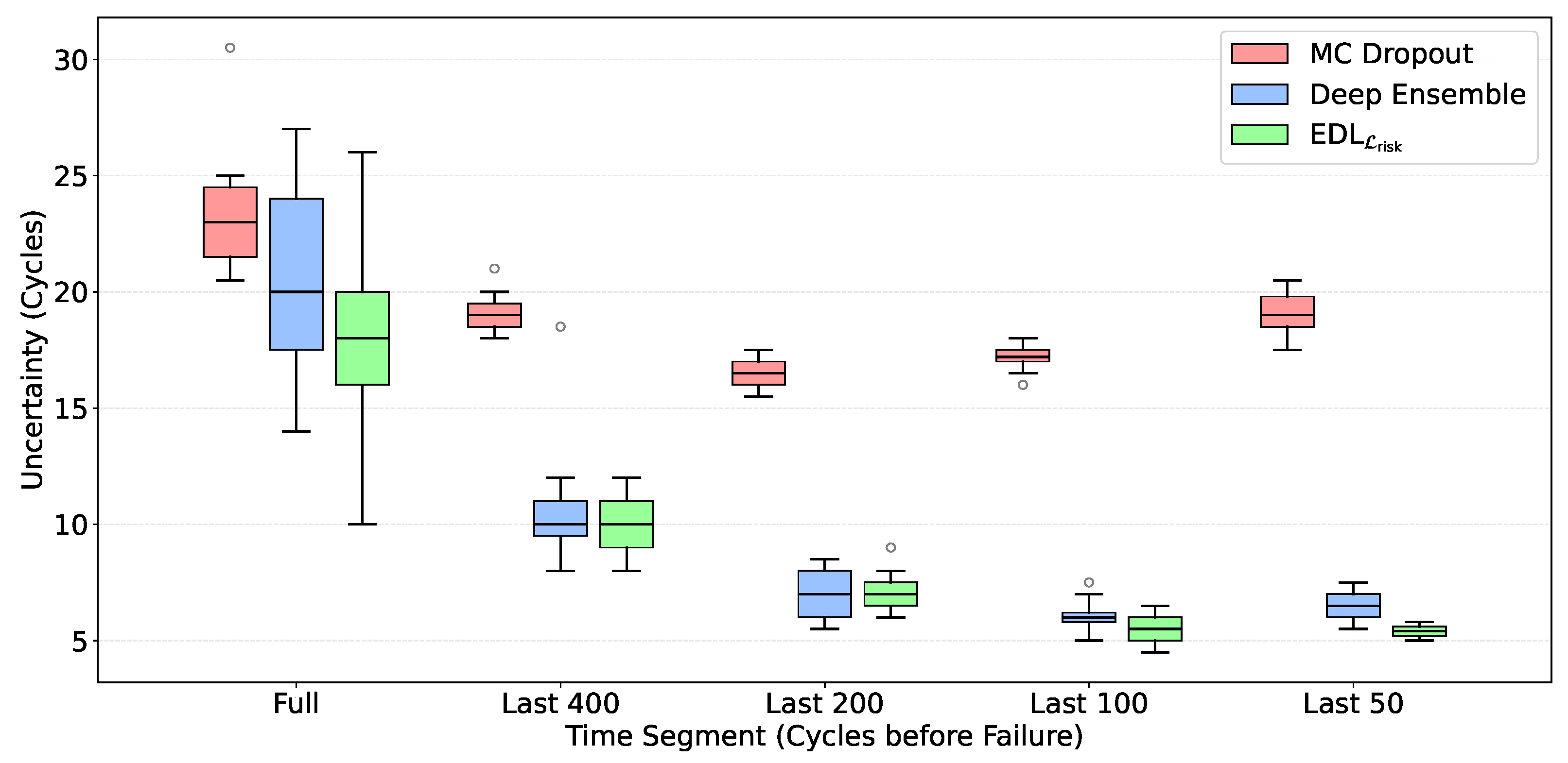
This behavior is illustrated in the grouped boxplot in Figure 4, where the ${\mathrm{EDL}}_{{\mathcal{L}}_{\mathrm{risk}}}$ model shows significantly tighter uncertainty distributions in the last 50 cycles compared to the baselines, while maintaining high coverage (PICP > 0.99). This characteristic is vital for reducing false alarms in predictive maintenance systems.

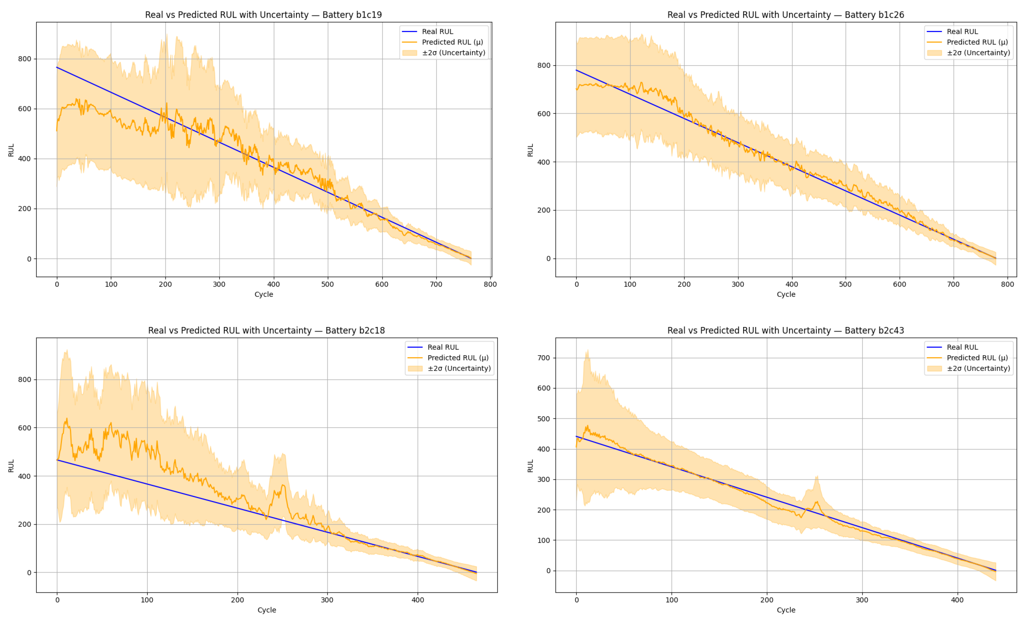
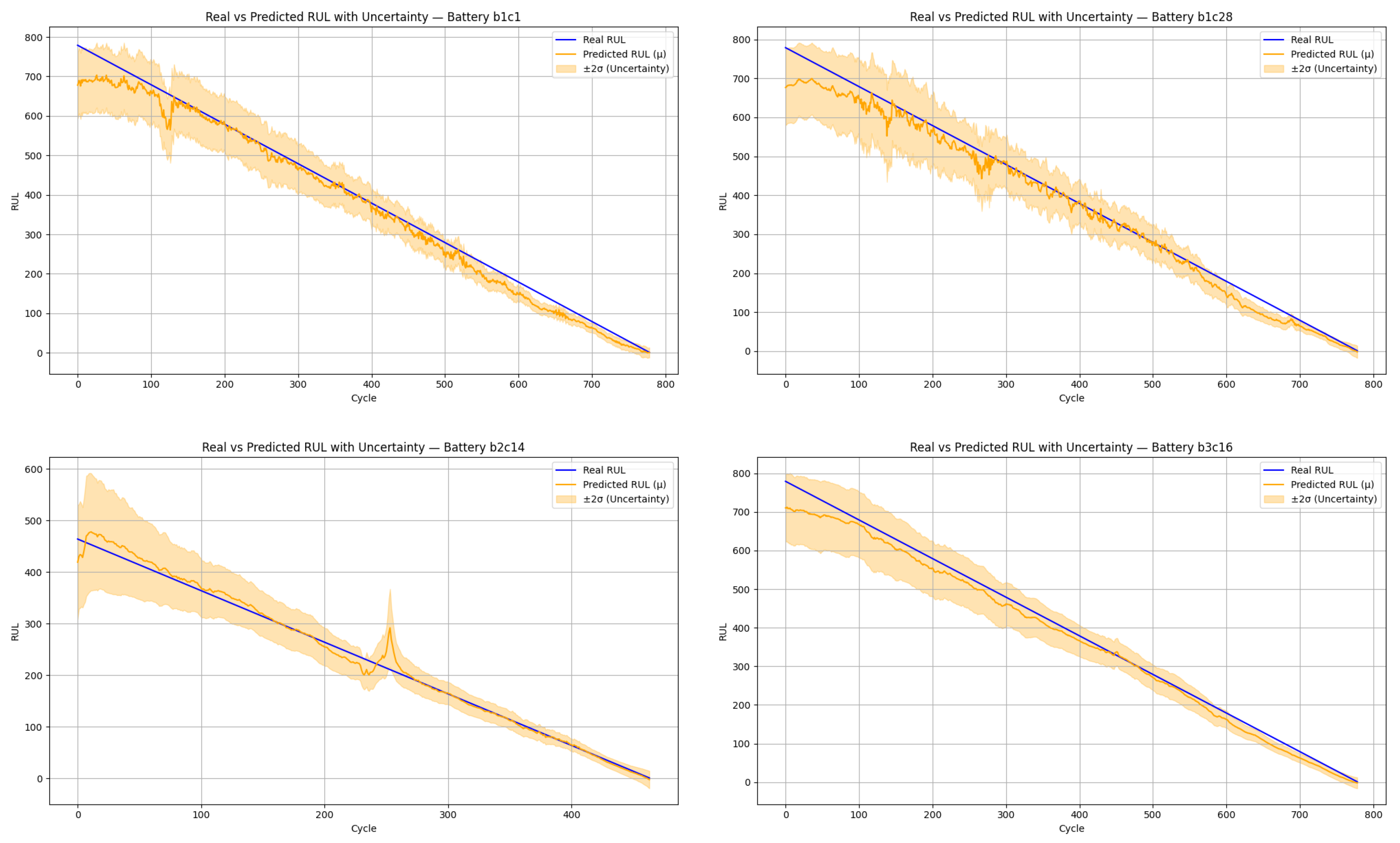
Finally, in Figure 5, we present predictions obtained with the ${\mathrm{EDL}}_{{\mathcal{L}}_{\mathrm{risk}}}$ model on four previously unseen batteries. The results show that both the prediction accuracy and the quality of the uncertainty estimates improve as the batteries approach their EoL. The higher uncertainty and less accurate predictions observed in the early stages may be attributed, on the one hand, to the proposed loss function, which assigns lower weight to prediction errors occurring at the beginning of the battery life and, on the other hand, to the fact that battery capacity curves are more similar in the initial cycles. Consequently, early-life battery behavior provides limited information for reliable RUL estimation during these phases. To further analyze the effect of the EDL framework, Figure 6 presents the predictions obtained for four batteries belonging to the training set. As expected, the model exhibits lower predictive uncertainty for these previously observed degradation trajectories compared to the unseen batteries in the test set. This behavior is consistent with the evidential learning paradigm, where uncertainty increases when the model encounters degradation patterns that were not observed during training, thereby reflecting epistemic uncertainty associated with limited prior evidence.

5.4. Impact of Data Cleaning

To evaluate the impact of data cleaning on model performance and uncertainty estimation, we compared the proposed ${\mathrm{EDL}}_{{\mathcal{L}}_{\mathrm{risk}}}$ model on two datasets: one with filtered input features using the rolling median method described in Section 4.1.1 and one without preprocessing. This comparison simulates the application of the proposed method on sensor data containing varying levels of noise, such as those arising from aging or improperly calibrated sensors.

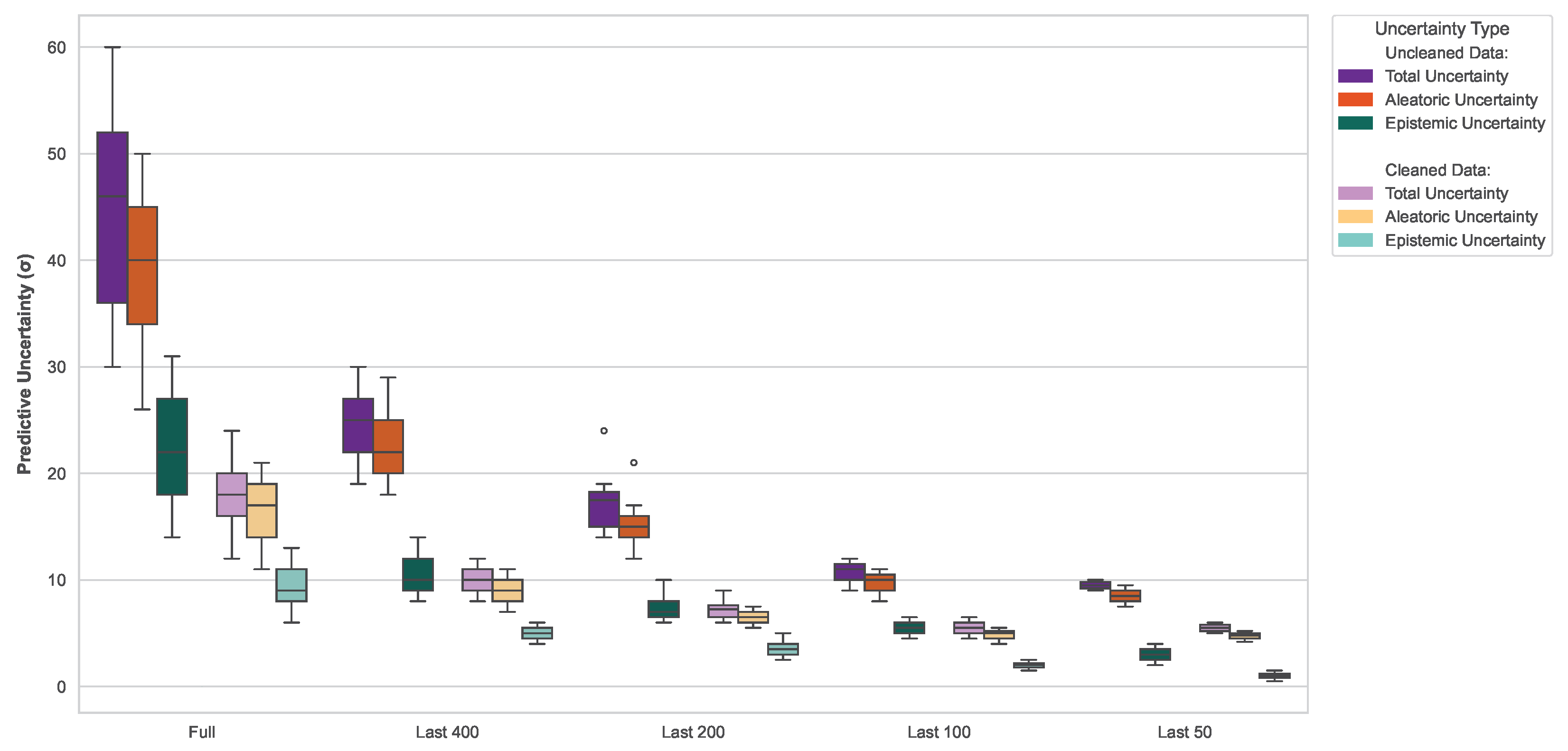
Leveraging the EDL framework, we were able to independently quantify aleatoric uncertainty, which stems from intrinsic noise and entropy in the input data, and epistemic uncertainty, which is attributed to the model’s knowledge and training limitations. The results, shown in Figure 7, clearly indicate that the model trained on cleaned data exhibits a significantly lower total uncertainty, which remains higher in the unfiltered dataset due to the presence of spurious peaks and drops in the input features.

In addition to uncertainty reduction, data cleaning also positively influenced the model’s predictive accuracy. As reported in

Table 7. Table of MAE values for the impact of data cleaning. Best results are in bold.

Training	MAE_Full	${\mathrm{MAE}}_{400}$	${\mathrm{MAE}}_{200}$	${\mathrm{MAE}}_{100}$	${\mathrm{MAE}}_{50}$
Cleaned	25.69	15.57	8.22	3.66	1.79
Uncleaned	29.01	17.89	9.47	4.69	2.83

, the model trained on cleaned data outperforms the one trained on uncleaned data across all time segments. Notably, on the full dataset, the MAE decreases from 29.01 to 25.69. Substantial improvements are also observed in the last 200 and 50 cycles, where MAE drops from 9.47 to 8.22 and from 2.83 to 1.79, respectively.

6. Discussion and Conclusions

The comparative analysis presented in the previous sections demonstrates that Evidential Deep Learning (EDL) provides substantial advantages over both MC Dropout and Deep Ensembles for uncertainty-aware RUL estimation. While Deep Ensembles achieve competitive prediction accuracy during the stable mid-life region of the battery, their probabilistic calibration remains limited: the coverage of their confidence intervals is consistently below the nominal level, and their epistemic uncertainty increases markedly near End-of-Life (EoL). In addition, ensemble-based inference requires multiple model evaluations, resulting in execution times an order of magnitude slower than EDL, which renders them less suitable for embedded battery management systems.

MC Dropout exhibits even poorer calibration, producing significantly underestimated predictive intervals due to its inability to explicitly model aleatoric uncertainty. As battery datasets naturally contain sensor-induced noise and nonstationary disturbances, the lack of an aleatoric component leads to systematic overconfidence and reduced robustness under input variability.

Within this landscape, EDL offers a unified probabilistic formulation capable of jointly estimating RUL and quantifying both epistemic and aleatoric uncertainties through a single forward pass. Among the EDL variants explored, the proposed model trained with the risk-aware loss ${\mathcal{L}}_{\mathrm{risk}}$ emerges as the best overall performer. This model not only achieves the lowest negative log-likelihood across the full degradation trajectory, indicating the most faithful probabilistic representation of the underlying failure process, but also maintains near-perfect coverage (PICP > 0.99) while producing narrower and more stable uncertainty bands during late-life operation. The ${\mathcal{L}}_{\mathrm{risk}}$ formulation explicitly penalizes underestimation of uncertainty in high-risk regions, guiding the model to allocate evidential mass more appropriately as the system approaches failure. This targeted emphasis enables superior accuracy and calibration in the final 100 and 50 cycles, where maintenance decisions are most critical.

A notable characteristic of the ${\mathcal{L}}_{\mathrm{risk}}$-trained model is its confidence convergence behavior: uncertainty decreases as degradation accelerates and the future trajectory becomes more predictable. This stands in direct contrast to Deep Ensembles and MC Dropout, whose uncertainty typically increases near EoL. Such convergence is particularly advantageous for predictive maintenance pipelines, as it yields more actionable and reliable information precisely when operational decisions must be made with high confidence.

The analysis of data-cleaning effects further reinforces the stability of the proposed EDL approach. Using the combined-loss model to decompose aleatoric and epistemic uncertainties revealed that noise in the input features disproportionately inflates aleatoric uncertainty, degrading both probabilistic calibration and prediction accuracy. Cleaned data therefore help the evidential framework form sharper and more consistent distributions, confirming the importance of preprocessing for real-world deployment.

Future work will extend the preliminary robustness assessment of Section 5.4 by systematically characterizing the behavior of the proposed ${\mathcal{L}}_{\mathrm{risk}}$-EDL model under controlled noise scenarios, sensor drift, and multi-channel degradation signatures. Additional efforts will investigate physics-informed evidential priors, adaptive loss-weighting strategies, and multimodal extensions for next-generation BMSs. Establishing these properties will further support the interpretation of EDL as a reliable measurement instrument capable of providing trustworthy RUL estimates and well-calibrated uncertainty quantification in practical industrial environments.