Cycle Aging Effect on the Inverse Open Circuit Voltage Curve of LiCoO₂ Batteries Under Different Voltage/SOC Conditions

Abstract

Lithium-ion batteries are widely used in applications ranging from portable electronics to electric vehicles and grid energy storage, owing to their high energy density, efficiency, and long lifetime. However, their performance degrades over time due to aging mechanisms such as solid electrolyte interface growth, lithium plating, and electrolyte decomposition, leading to capacity fade and reduced power capability. Accurate state of charge (SOC) estimation is therefore essential for ensuring safe and efficient battery operation, particularly within battery management systems. While many existing methods rely on the direct relationship between open circuit voltage (OCV) and SOC, practical applications require the inverse mapping, i.e., the estimation of SOC from measured OCV values. This inversion is not always straightforward: analytical solutions are only available for simple models, whereas more accurate formulations often require computationally intensive numerical methods. Direct analytical SOC–OCV relationships (inverse OCV–SOC models) provide an effective alternative, enabling simplified SOC estimation without numerical inversion. Previous work proposed a direct generalized Gaussian analytical relationship expressing the absolute state of charge as a function of OCV, thereby simplifying SOC estimation and avoiding numerical inversion, developed and validated on a lithium cobalt oxide battery cycled in the linear region of the OCV curve at constant battery temperature. Building upon this study, the proposed approach was extended to investigate the effects of cycle aging across a wider operating range, considering low, medium, and high voltage/SOC conditions. The model was experimentally validated, at constant battery temperature, on the same type of lithium cobalt oxide batteries through an extensive testing campaign, demonstrating its effectiveness in capturing battery behavior under different operating conditions.

1. Introduction

Among rechargeable batteries, lithium-ion batteries (LiBs) are one of the most widely used energy storage systems in many applications. These range from small portable devices (smartphones, notebooks, medical tools, etc.) to larger ones, such as electric vehicles (EVs). On the other hand, LiBs are also used in stationary applications to support renewable energy sources and offer different services to the grid, interfaced through power converters [1,2,3]. The widespread use of these energy storage systems is not only due to their high energy and power density, high efficiency, relatively long lifetime, and lack of memory effect [4,5] but also to the goal of reducing carbon emissions, pollution, and addressing the climate crisis [6].

On the other hand, depending on the storage or operating conditions, LiBs undergo different aging mechanisms, such as solid electrolyte interface (SEI) growth, lithium plating, and electrolyte decomposition, which lead to different aging modes (loss of lithium inventory, loss of active material, loss of electrolyte, and conductivity loss) and, ultimately, to practical consequences such as capacity fade and power reduction [7]. To limit this degradation, especially during battery usage, it becomes very important to model these devices in order to estimate and predict how a LiB may evolve under certain conditions. For this reason, such models can be implemented in battery management systems (BMS), which can perform these estimations in real time. Specifically, accurate state of charge (SOC) estimation is crucial for ensuring safe battery operation by limiting the operating conditions within safe voltage limits and minimizing degradation.

SOC can be estimated using either non-model-based or model-based approaches [8]. Among the non-model-based methods, Coulomb counting is one of the most commonly used because of its simplicity. Nevertheless, its accuracy strongly depends on the precision of the current measurement, and even small sensor errors may accumulate and lead to significant estimation drift [9].

Model-based approaches can be divided into three main categories. White-box models are based on the physical and chemical mechanisms underlying the battery and are usually described by partial differential equations. They can provide very accurate predictions but are difficult to implement in BMS due to their high complexity and computational requirements [10,11]. In contrast, black-box models are simpler but generally less accurate, as they rely on data-driven approaches in which large experimental datasets are used to derive analytical relationships. Today, machine learning techniques are increasingly applied within this category, including neural networks [12,13], relevance vector machines [14,15], and support vector machines [16,17]. Gray-box models, on the other hand, represent a compromise between the two approaches, combining the simplicity of data-driven methods with the relatively high accuracy of physics-based models. Examples include equivalent electric circuit models, which retain an underlying physical interpretation but whose parameters are experimentally determined, and adaptive filter-based models, where the model is continuously updated using feedback from the current output, such as in Kalman filter-based methods or recursive least-squares approaches [18,19,20].

In any case, another frequently adopted method among black-box models relies on the analytical relationship between the open circuit voltage (OCV) and SOC. This approach generally provides higher accuracy and can also be used to recalibrate Coulomb counting results. However, it is difficult to apply directly in online conditions, since determining the OCV requires the battery to remain at rest for a sufficiently long period of time [21]. As an alternative, the OCV value can be measured during a resting period or estimated through battery models, often based on gray-box approaches, where the reliability of the SOC estimation is closely related to the accuracy of the adopted model [22].

In this context, OCV–SOC relationships can be represented either by look-up tables or by analytical expressions. Table-based approaches are straightforward but require a large amount of experimental data, which is not always available, and considerable memory resources [23]. Analytical formulations, on the other hand, reduce the number of required OCV data points and may be expressed through polynomial, logarithmic, exponential, or hybrid functions [24,25,26,27], with their computational burden depending on the number of parameters involved.

Nevertheless, factors such as temperature and battery degradation [28] lead to variations in the actual battery capacity and in the OCV–SOC relationship. Therefore, it is important to analyze how these quantities evolve under different operating conditions, as addressed in many studies in the literature.

For example, in [29], a lithium iron phosphate battery was subjected to cycle aging, and the SOC was adjusted according to the actual available capacity, thereby accounting for the impact of cycle aging on the OCV–SOC relationship. Specifically, the authors found that the different OCV–SOC curves were almost overlapping after the correction. In [30], the authors corrected the OCV–SOC curve of an aged battery by adding a correction factor to the original OCV–SOC curve obtained at the beginning of the battery’s life. In [31], the authors combined the Coulomb counting method for SOC estimation with information about the relationship between the degradation level of the LiB and SOC derived from different OCV–SOC curves.

Temperature effects on the OCV–SOC relationship have also been investigated in several studies. A simple analysis was conducted in [32], where the authors considered the temperature effect on the OCV–SOC curve through a look-up table. In [33], different OCV–SOC relationships for various lithium-ion battery chemistries were corrected for temperature variations using an appropriate correction factor. In [34], the authors examined the impact of temperature on the OCV–SOC curve and derived a function to compensate for capacity variations with temperature for a lithium nickel manganese cobalt oxide battery.

Considering the previous discussion, many studies have examined the direct relationship between OCV and SOC, or alternatively between OCV and the state of discharge. This means that, given a SOC value, the corresponding OCV can be directly obtained.

However, in practical applications, the main interest lies in determining the SOC from a measured OCV. This implies reversing the OCV–SOC relationship, which is not always straightforward. Analytical inversion is only feasible when the original function has a relatively simple mathematical form. For instance, the Unnewehr model [35] and its piecewise extension [36] can be inverted without difficulty. Nevertheless, the accuracy of the resulting SOC estimation still depends on how precisely the initial OCV–SOC model represents the battery behavior under the conditions for which it was derived. When more complex formulations are used to describe the OCV–SOC relationship, numerical techniques, such as Newton–Raphson, bisection, and Lagrange inversion, are typically required to obtain the inverse function, which may introduce additional computational effort [37]. Specifically, the Newton–Raphson method consists of an iterative procedure for computing the inverse of a function. First, an initial guess of the SOC is provided, and the SOC value is subsequently updated through successive iterations until the calculated OCV converges to the target value within a prescribed tolerance. The bisection method progressively halves the search interval and identifies the sub-interval containing the solution. This process is repeated until the sub-interval is sufficiently small to approximate the desired value. The Lagrange inversion method represents the inverse function as a power series expansion.

Directly creating inverse OCV–SOC relationships, i.e., direct SOC–OCV functions, can provide notable advantages, such as simplifying SOC estimation and enhancing error assessment. However, such direct SOC–OCV formulations are still relatively scarce in the literature. In [38], a piecewise linear SOC–OCV function was used in an inverted Coulomb counting approach for SOC determination in a fresh lithium cobalt oxide (LCO) battery. Meanwhile, the authors’ previous work in [39] proposed a new analytical model based on a double Gaussian function that directly captures the inverse relationship, allowing SOC estimation from measured OCV values without requiring numerical inversion, specifically for LCO batteries. That study also investigated how the function varies with battery temperature for a fresh cell. Conversely, in [40], the authors extended that model using a double generalized Gaussian function, investigating how the function evolves with cycle aging under constant battery temperature conditions during both aging and characterization, enabling the estimation of the actual battery capacity, but only for a battery operated within a limited SOC range. Specifically, the cell was cycled exclusively within the approximately linear portion of the OCV curve, corresponding to the medium SOC range (20–80%), with the voltage constrained between 3.45 V and 4.05 V. As a result, the behavior outside these limits was not captured. Therefore, extending those findings to batteries cycled beyond this region deserves further investigation.

In light of the above, the approach presented in [40] was extended in this work to investigate cycle aging in the same type of LCO battery across three distinct operating voltage/SOC conditions: low, medium, and high. Specifically, the absolute state of charge, q, is modeled as a function of the OCV and then validated through an extensive experimental campaign. In this case as well, the present study intentionally considered isothermal conditions during both aging and characterization to isolate the effect of voltage/SOC from that of temperature.

As a result, the proposed formulation enables direct evaluation of battery capacity and SOC without relying on extensive look-up tables or numerical inversion, thus reducing memory requirements and computational complexity. This makes the model particularly suitable for real-time applications, such as onboard BMS.

2. OCV Curve Estimation

According to the objective of the present study, the relationship linking the absolute state of charge, q, to the OCV—evaluated at different cycling levels and operating conditions—can be modeled by experimentally estimating the OCV profiles obtained during battery discharge.

From a fundamental standpoint, the OCV can be measured at the battery terminals only when the cell is at chemical equilibrium. This condition is achieved when the battery is allowed to rest for a sufficiently long time. During battery operation, voltage drops associated with various polarization phenomena occur, giving rise to electrical transients that must decay before the equilibrium voltage can be measured.

The two main experimental methods used to obtain the q–OCV curve are the galvanostatic intermittent titration technique and pseudo-OCV tests. The former subjects the battery to partial discharge steps followed by sufficiently long rest periods, allowing the battery to reach chemical equilibrium. The voltage measured at the end of each rest period can then be considered the OCV, and the collection of these points forms the q–OCV curve.

In contrast, pseudo-OCV tests discharge the battery at a very low current, making it possible to approximate the terminal voltage as the OCV. Both methods, however, require a considerable amount of time to perform. For this reason, as suggested in previous work [40], a good compromise can be achieved by discharging the battery at a 1C rate and then estimating and subtracting the overpotentials from the measured voltage.

These overpotentials arise from different electrochemical phenomena associated with processes occurring at different frequency ranges. At high frequencies, the overpotential is mainly related to the ohmic resistance of battery components, including the electronic conductivity of the electrodes and current collectors, as well as the ionic conductivity of the electrolyte. At medium–high frequencies, the overpotential is associated with the additional interfacial resistance of the SEI, commonly referred to as SEI polarization. In the medium-frequency range, the overpotential is governed by the reaction kinetics at the electrode–electrolyte interface, which include charge-transfer processes and double-layer effects. Finally, at low frequencies, the overpotential is mainly attributed to mass transport limitations caused by lithium/lithium ions diffusion processes in both the electrodes and the electrolyte.

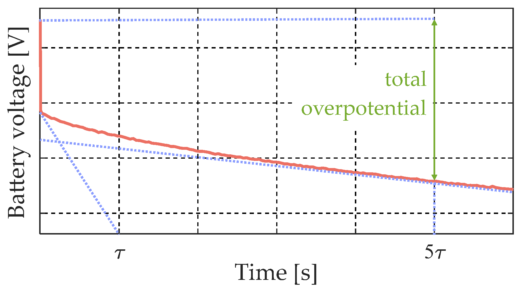
When the battery reaches the steady state and all the electric transient associated with the above dynamics are finished, the total overpotential over the whole internal battery resistance can be estimated. At the start of the battery discharge at a constant current, the output battery voltage exhibits a transient response caused by the above-mentioned electrochemical processes occurring within the cell. By selecting a suitable time interval after this initial transient—specifically considering the slowest process, i.e., when lithium/lithium ions diffusion can be assumed to have reached a quasi-steady condition—the total overpotential of the battery can be evaluated, as illustrated in Figure 1.

This procedure assumes that the internal resistance does not significantly vary with SOC. Although some SOC dependence generally exists, the variation is typically small at room temperature (20–30 °C) [41]. In particular, for LCO batteries operating across nearly the entire SOC range, the resistance remains almost unchanged, even under different levels of cycling-induced aging [42]. Moreover, this approximation does not affect the general validity of the proposed modeling approach, which is independent of the specific method used to extract the OCV. From an application perspective, the OCV can be more accurately determined either under relaxed conditions (i.e., after sufficient rest time) or by adopting a model that explicitly accounts for internal resistance and overpotentials. Therefore, the proposed modeling framework can be directly combined with more accurate OCV estimation techniques without modification. Finally, regarding cycle aging, the total overpotential is reidentified at different stages of battery life.

After estimating the total overpotential and reconstructing the q–OCV relationship, the section of the curve corresponding to the selected transient interval was removed from the analysis.

In the proposed q–OCV model, the absolute state of charge, q, is defined as the time integral of the battery current, i_bat (positive during charging), as follows:

$$q(t)={\displaystyle \frac{1}{3600}}{\displaystyle {\displaystyle \underset{0}{\overset{t}{\int }}}{i}_{bat}\cdot d\tau }+q(0)$$

(1)

where q(0) represents the initial value of the absolute state of charge. By dividing (1) by the actual battery capacity, C_bat,a, the SOC can be obtained:

$$\mathrm{SOC}={\displaystyle \frac{q}{C_{bat,a}}}$$

(2)

The double generalized Gaussian analytical function proposed in [40] to describe the q–OCV relationship was adopted in this work and further extended to incorporate different operating conditions:

$$q(\mathrm{OCV})=p_{1,1}(Q)\cdot e^{-{\left({\displaystyle \frac{\mathrm{OCV}-p_{1,2}(Q)}{p_{1,3}(Q)}}\right)}^2}+p_{2,1}\cdot e^{-{\left({\displaystyle \frac{\mathrm{OCV}-p_{2,2}(Q)}{p_{2,3}(Q)}}\right)}^6}$$

(3)

The parameters p_1,1, p_1,2, p_1,3, p_2,1, p_2,2, and p_2,3, capture how the OCV curve evolves with cycle aging. The latter is quantified using the cumulative charge exchanged with the battery as an indicator of the cycling level:

$$Q(t)={\displaystyle \frac{1}{3600}}{\displaystyle {\displaystyle \underset{0}{\overset{t}{\int }}}\left|i_{bat}\right|\cdot d\tau }.$$

(4)

3. Experimental Procedure and Setup

The battery used in this study was the LCO pouch cell model 8,773,160 K (10 Ah, 2.75–4.2 V), manufactured by General Electronics Battery Co., Ltd. (Shenzhen, China). Specifically, three cells from the same batch were cycled and tested in three different voltage/SOC conditions: low, medium, and high. In this way, it was possible to analyze how the q–OCV curve evolves as a function of the cycling level under different operating voltage/SOC ranges.

3.1. Experimental Setup

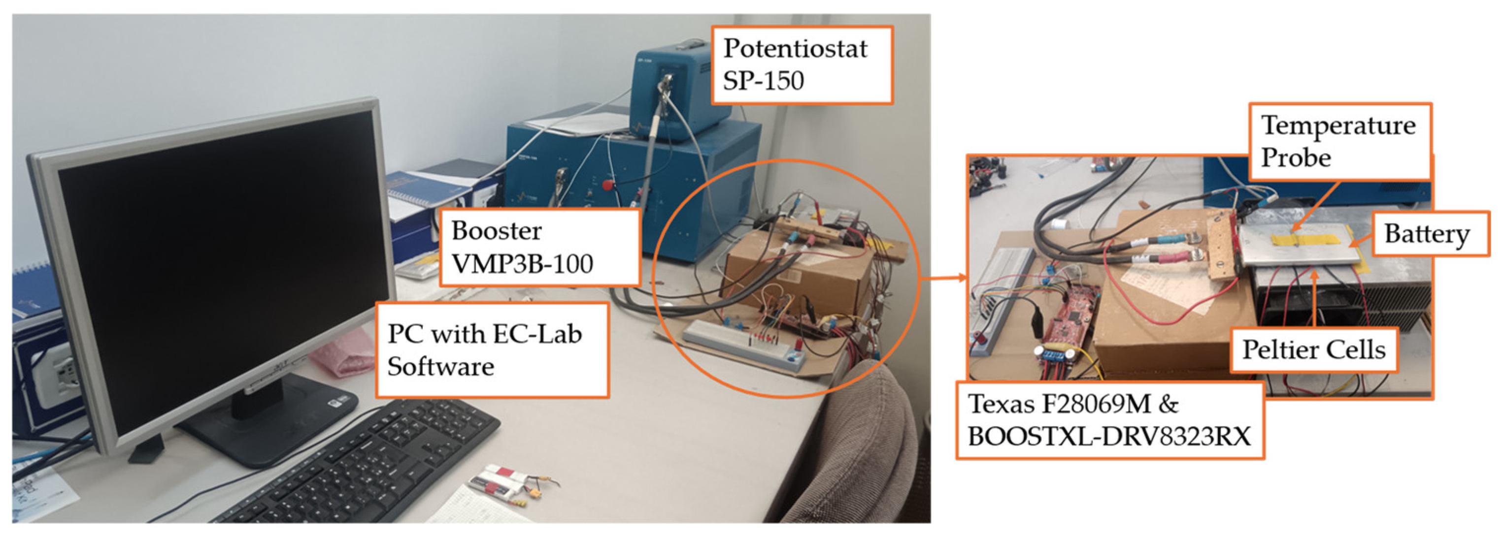
Figure 2 illustrates the experimental apparatus adopted for the tests. It consists of a potentiostat (SP-150) coupled with a 100 A booster module (VMP3B-100), both produced by Bio-Logic Science Instruments. These devices were connected to a personal computer via an Ethernet interface and operated using the EC-Lab software (version 11.34). The booster unit supplied the required current to the battery under test through dedicated power cables.

The battery testing platform also incorporated a thermal management system designed to actively maintain the battery temperature at a constant value of 25 °C throughout the entire experimental campaign, including both the aging cycles and the discharge tests used to reconstruct the q–OCV curves. No significant temperature fluctuations were observed during the tests. Maintaining a stable temperature was necessary to minimize temperature-induced variations in the q–OCV curve.

Specifically, three Peltier modules were installed between the tested battery and a heatsink equipped with two cooling fans. These modules were regulated through the Texas Instruments BOOSTXL-DRV8323RX converter, which was controlled by a Texas Instruments F28069M microcontroller board. Specifically, the battery temperature was measured using a Pt100 temperature probe placed on the top surface of the battery. The measured temperature was continuously compared with the reference value (25 °C), and the resulting temperature error was used as input to a proportional–integral controller implemented on the Texas Instruments F28069M microcontroller board. The controller output was then used to generate the duty cycle for the Texas Instruments BOOSTXL-DRV8323RX converter, which supplied the appropriate current to the Peltier cells.

3.2. Experimental Procedure

The three batteries under test underwent two experimental phases. The first phase consisted of the OCV curve characterization and was performed when the batteries were fresh and after each occurrence of the second phase, namely the cycling phase.

The OCV curve characterization phase consisted of subjecting the batteries under test to a constant current–constant voltage (CC–CV) charging protocol followed by a constant current (CC) discharge, both carried out using the potentiostat coupled with the 100 A booster module. During charging, the CC–CV profile was applied by first charging the battery in CC mode at 10 A (1C). This stage ended when the battery voltage reached the maximum cutoff value of 4.2 V. The protocol then switched to CV mode, maintaining the same voltage until the current dropped below 500 mA (0.05C), at which point the battery was considered fully charged. Subsequently, the discharge phase was performed in CC mode at 10 A (1C) and terminated when the battery voltage reached the minimum cutoff value of 2.75 V.

Once the batteries were fully discharged and before starting the cycling phase, each battery was charged to a different SOC level according to the voltage/SOC condition in which it was to be cycled. Specifically, the battery assigned to the low voltage/SOC condition was charged at 10 A (1C), transferring 1 Ah, corresponding to 10% of SOC relative to the nominal capacity. The battery assigned to the medium voltage/SOC condition was charged at 10 A (1C), transferring 5.2 Ah, corresponding to 52% of SOC. Finally, the battery assigned to the high voltage/SOC condition was brought to 90% of SOC.

At this point, the three batteries entered the cycling phase, which consisted of a sequence of charge and discharge steps performed at a constant current of 20 A (2C). The cycling was restricted according to the three predefined voltage/SOC conditions. These limits were imposed by setting maximum SOC variations and corresponding voltage boundaries, as reported in

Table 1. Voltage/SOC condition limits.

Voltage/SOC Condition	SOC Limits	Voltage Limits
Low	6–10%	2.75 V–3.65 V
Medium	48–52%	3.60 V–3.95 V
High	90–94%	3.90 V–4.20 V

. Each cycling phase transferred approximately 500–1000 Ah, resulting in a total cumulative charge exchange of about 20 kAh over 29 cycling phases for each voltage/SOC condition.

It is worth noting that the 2C current rate already represents a relatively demanding operating condition, thus inherently including aspects related to high-power operation and fast charge/discharge regimes. Therefore, while the experimental campaign was carried out under controlled conditions, it is not limited to mild operating scenarios.

The selection of relatively narrow voltage/SOC ranges was made intentionally to ensure a well-controlled experimental framework and to isolate the effect of low, medium, and high voltage/SOC ranges on the investigated aging behavior. In particular, the low and high voltage/SOC ranges were kept limited in order to operate the battery within regions where the OCV curve is very steep, close to the voltage limits of the battery. For consistency and a fair comparison across the three investigated operating ranges, a similarly narrow interval was also adopted for the medium voltage/SOC case. Therefore, although such narrow SOC cycling does not fully represent real-world applications, such as EV operation—where much wider SOC ranges are typically experienced—this experimental design allowed us to focus on the dependence of the observed behavior on the voltage/SOC level itself.

Moreover, it should be noted that, if the voltage limits were reached before the prescribed SOC variation was achieved, the amount of charge exchanged during a cycle could change as the battery aged. Nevertheless, previous studies provide useful insights regarding the influence of cycling conditions on degradation, particularly in terms of capacity fade. Specifically, the results reported in [43] indicate that, within the approximately linear region of the OCV curve (20–80% of SOC) and at constant battery temperature, capacity fade is not significantly affected by the specific SOC interval or by the shape of the charge–discharge cycle. Furthermore, the analysis presented in [44] show that, under similar conditions—particularly with battery temperature controlled using Peltier cells, as in the present study—the current rate used during charging and discharging does not have a noticeable impact on capacity fade. Specifically, the type of LCO battery used in the present work is the same as that considered in [43,44]. Consistent results are also observed in [45], where a similar weak dependence on current rate was found. Additionally, the work in [46] demonstrates that, when the SOC interval is fixed, the dominant factor influencing capacity fade is the average SOC level. Specifically, within the 20–80% of SOC range, capacity fade is nearly independent of the exact SOC subrange, whereas outside this interval—i.e., beyond the linear region of the OCV curve—the degradation rate differs.

Based on these considerations, it is reasonable to assume that battery degradation can be primarily related to the cumulative exchanged charge, Q, regardless of the specific cycle shape and mean SOC value, provided that the operating voltage/SOC range lies within one of the three defined regions of the OCV curve (i.e., low, medium, or high voltage/SOC conditions). This supports the potential applicability of the proposed modeling framework also under variable cycling profiles, although this was not directly validated in the present work.

4. Model Characterization, Validation, and Results Discussion

According to the experimental procedure described in the previous section, several discharge voltage curves were recorded for each voltage/SOC condition at different cycling levels. Specifically, the experimental absolute state of charge values, q_exp, corresponding to the experimental OCV values, OCV_exp, were obtained by applying the measured battery current in (1). The experimental q–OCV curves were then obtained from these data by removing the total battery overpotential, as discussed in Section 2. Specifically, a time interval of 50 s was used to allow the electrical transients to decay, based on the diffusion dynamics of the batteries.

To validate the proposed q–OCV model across the different voltage/SOC conditions, a subset of the experimental q–OCV curves was used for model characterization, while the full dataset was employed for validation.

4.1. Characterization of the Model

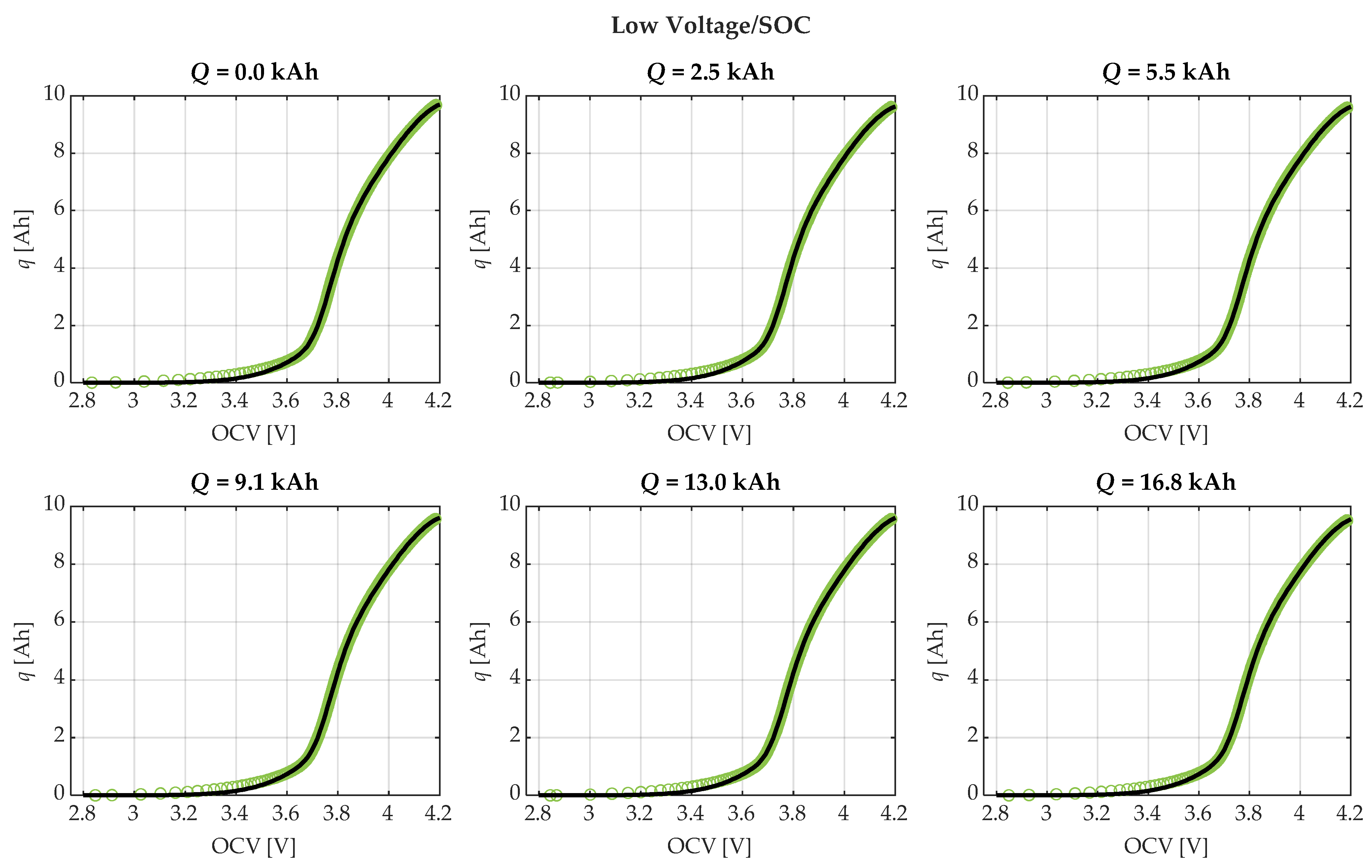
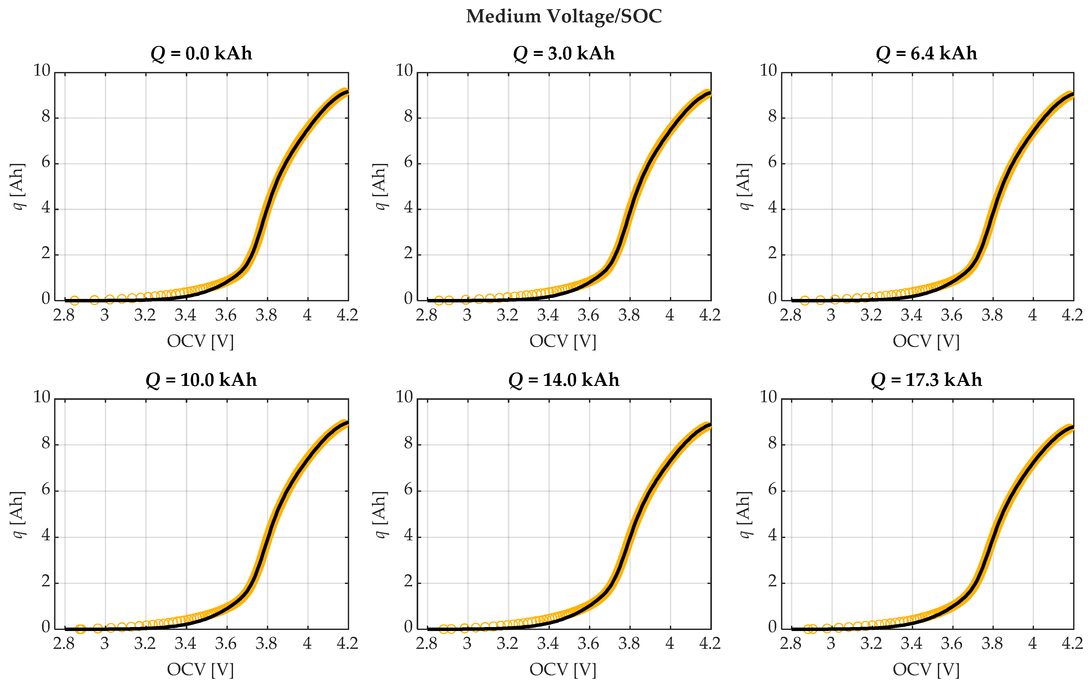
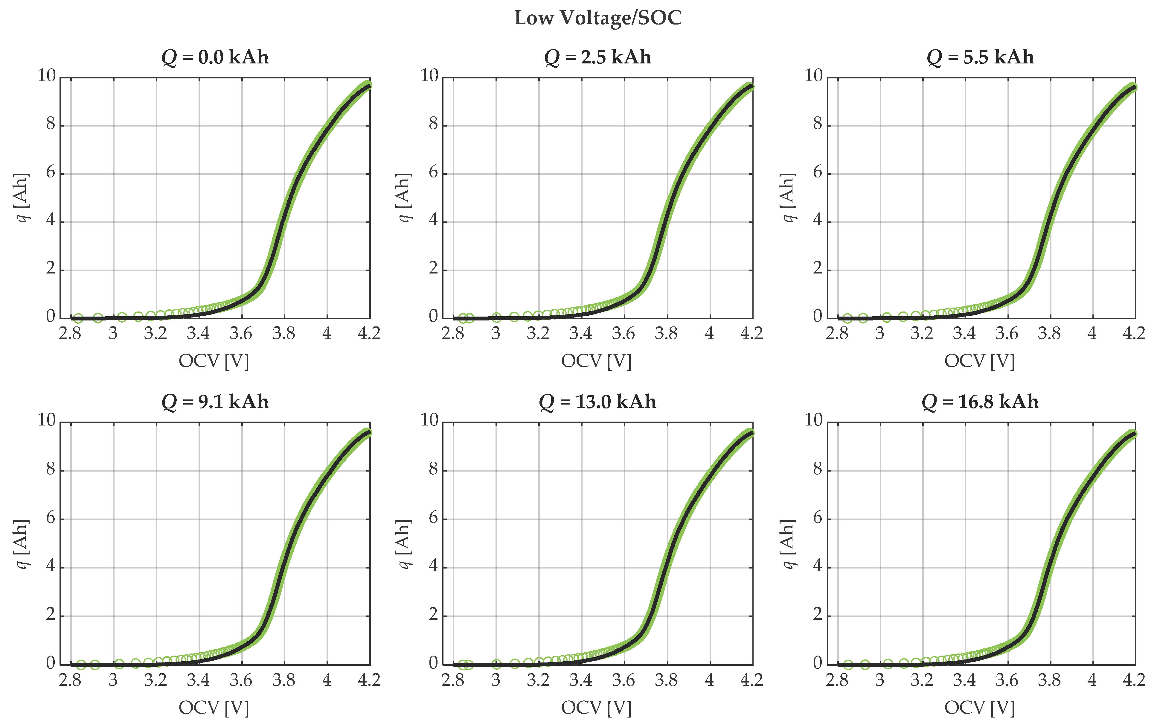
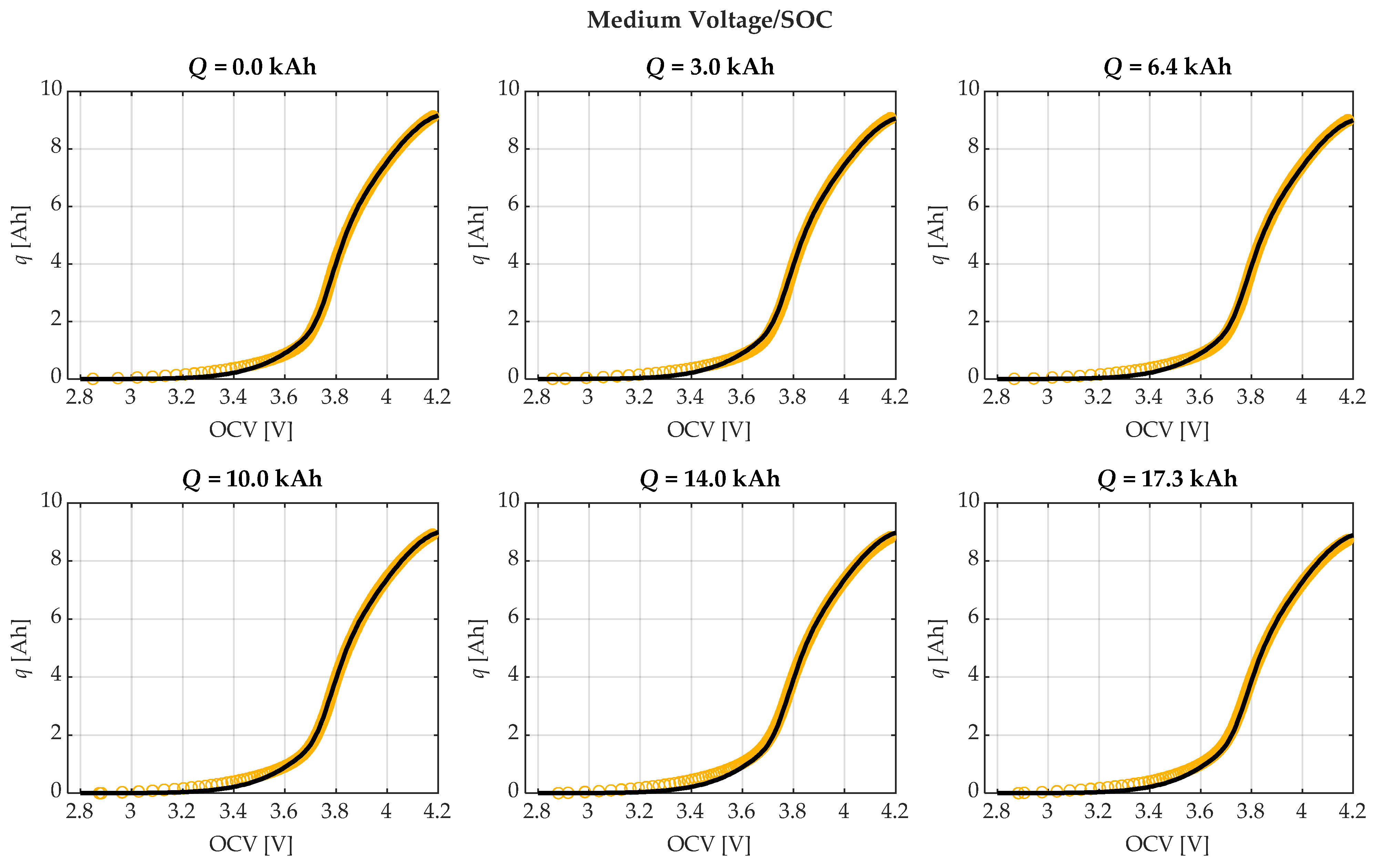
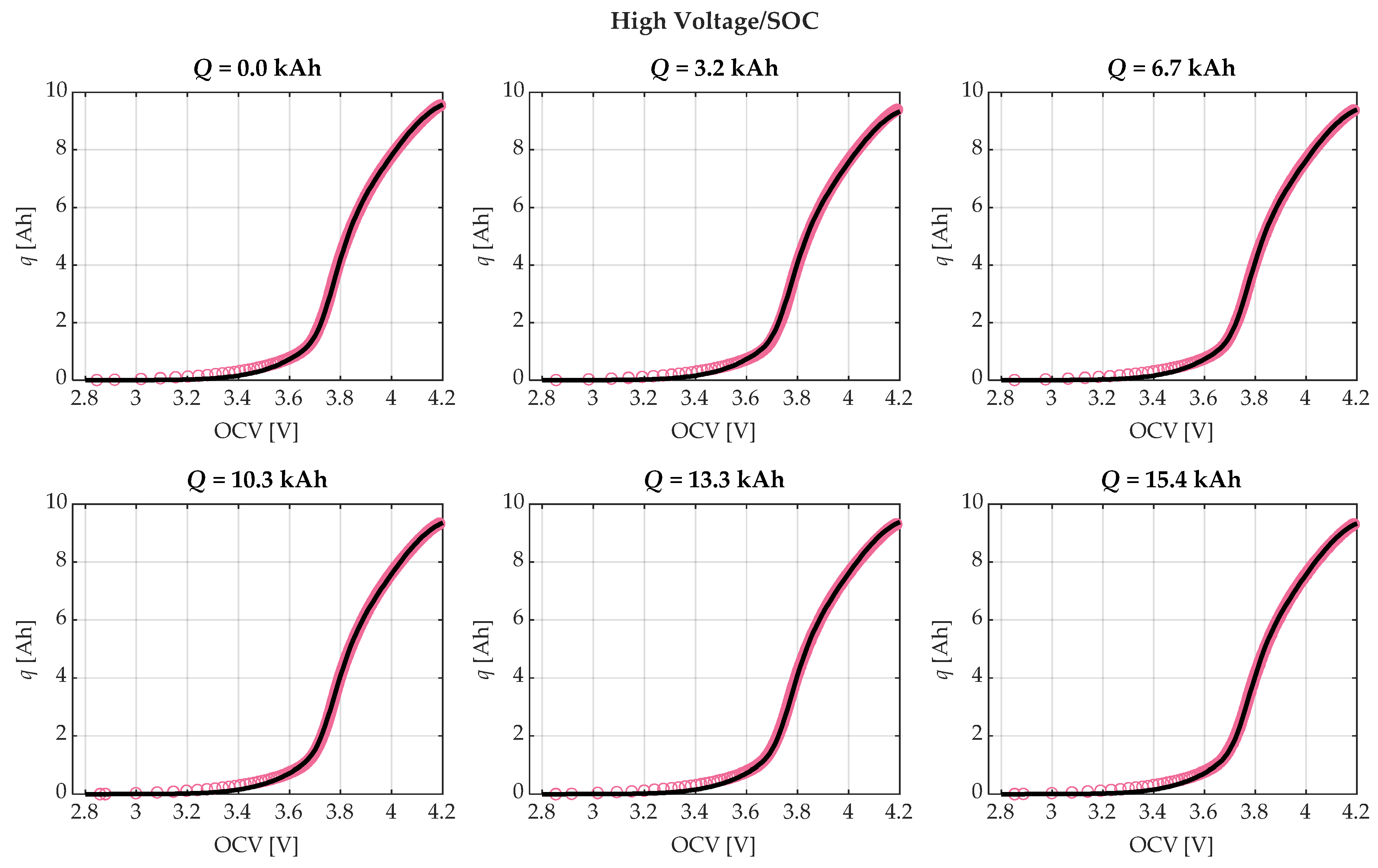
Specifically, six q–OCV curves for each voltage/SOC condition were selected to ensure approximately uniform spacing across the different cycling levels. The objective was to determine the parameters of (3) as a function of the cycling level, Q. To achieve this, least-squares methods were applied. Since the proposed analytical model includes parameters within exponential terms, the resulting problem is nonlinear. Therefore, a nonlinear least-squares approach was employed using the “fit” function in MATLAB (2022b).

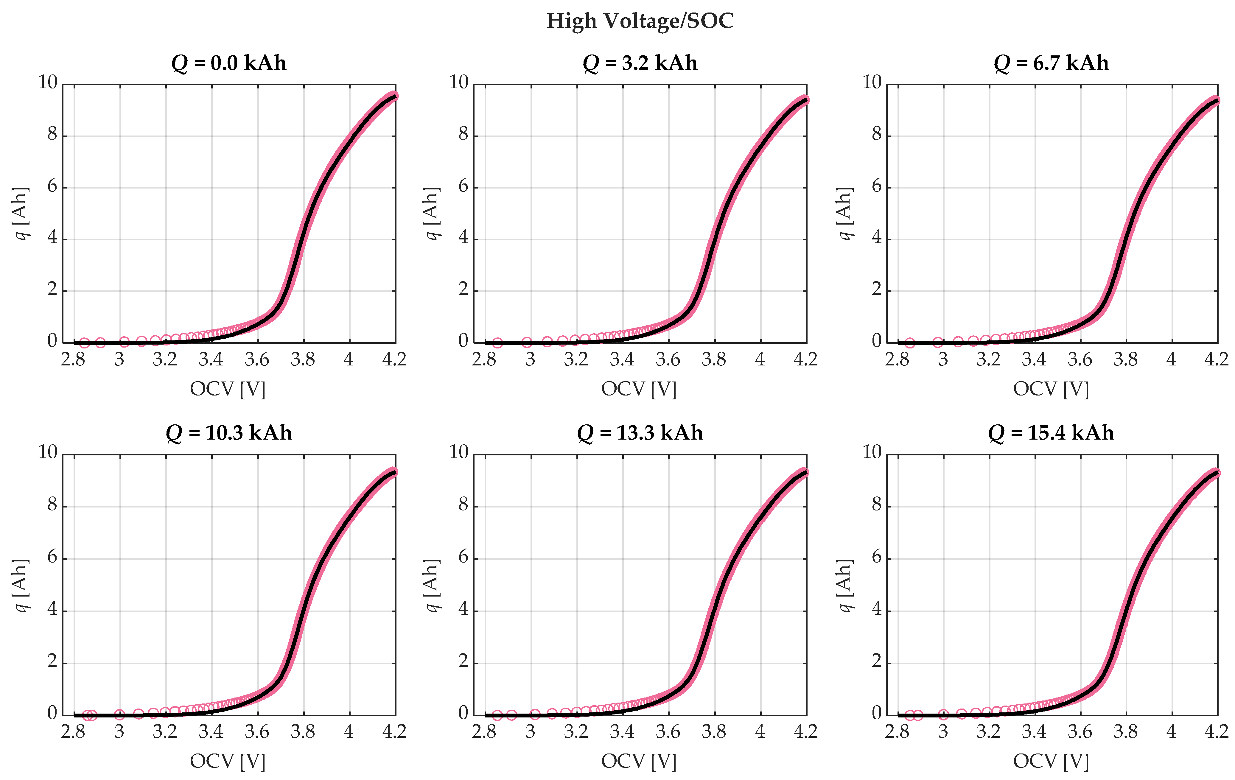
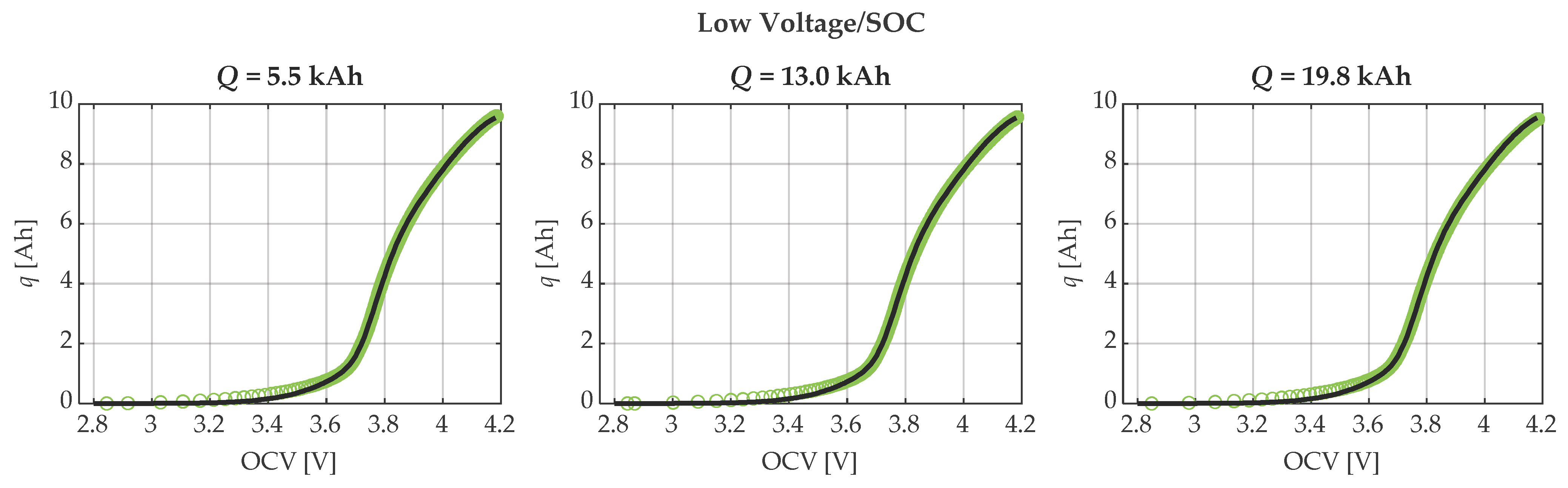
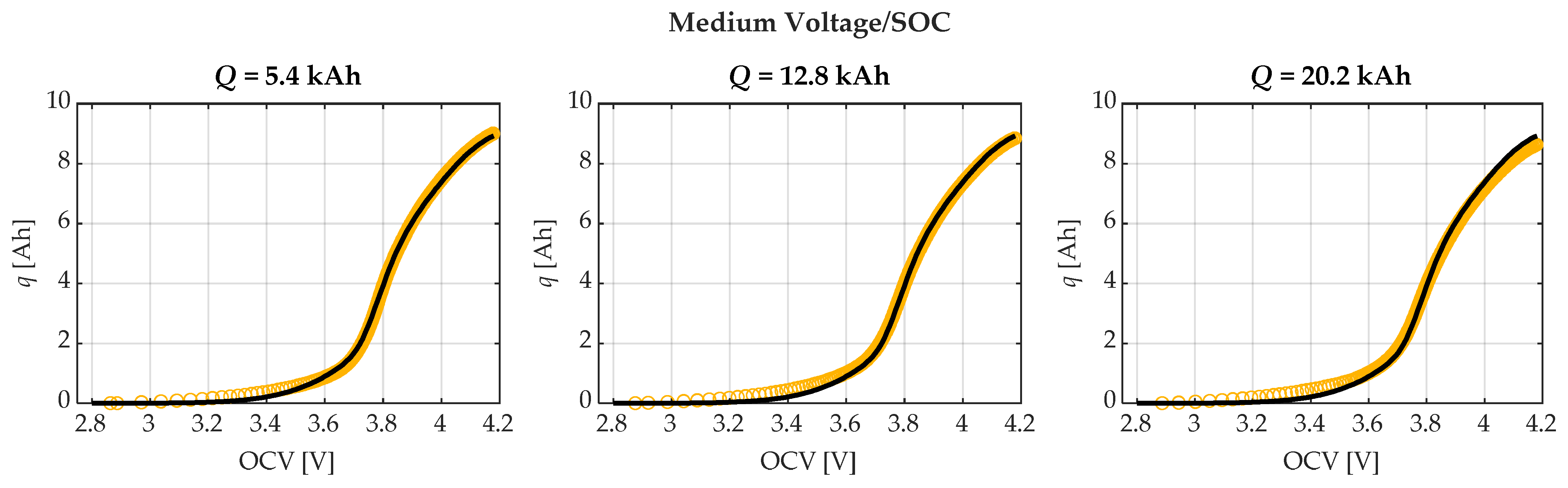
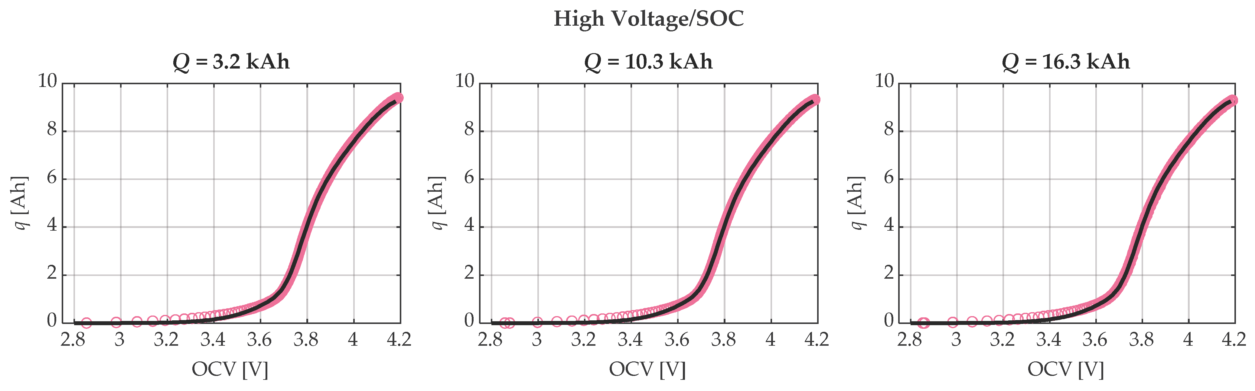
The results of these fitting procedures, along with the corresponding experimental data, are shown in Figure 3, Figure 4 and Figure 5, where a good agreement can be observed for all cases.

Additionally, the coefficient of determination (R²) was calculated. The obtained R² values confirm the accuracy of the proposed model, as they exceed 0.9996 across all cycling levels and for each voltage/SOC condition.

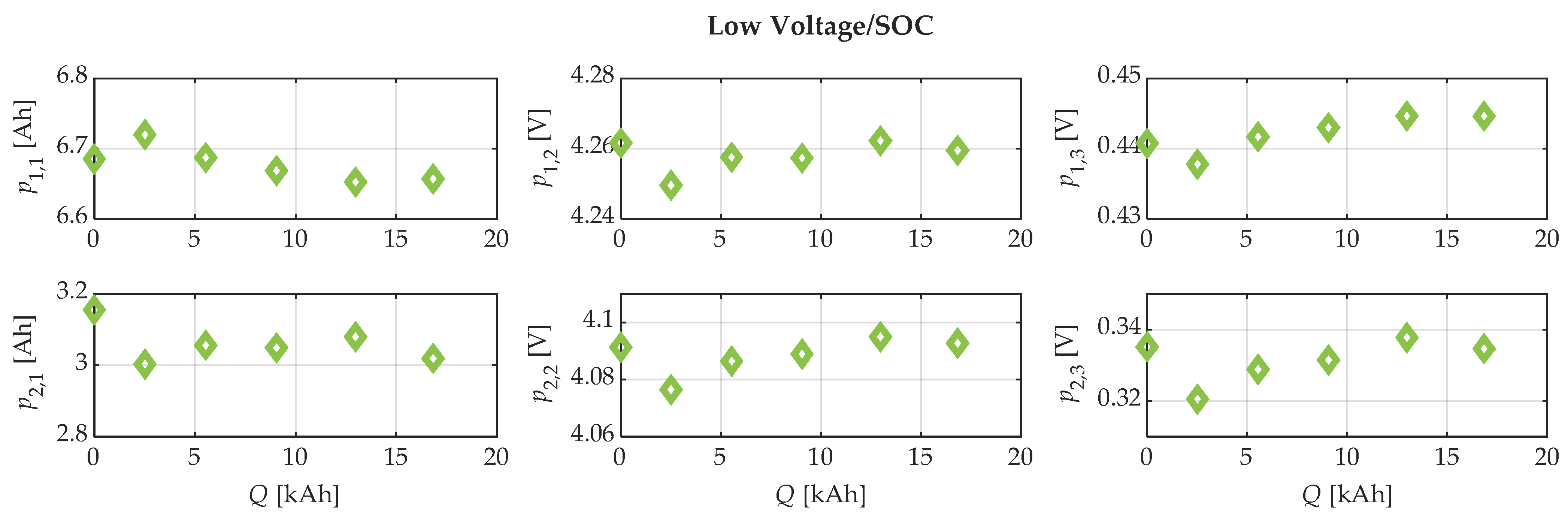
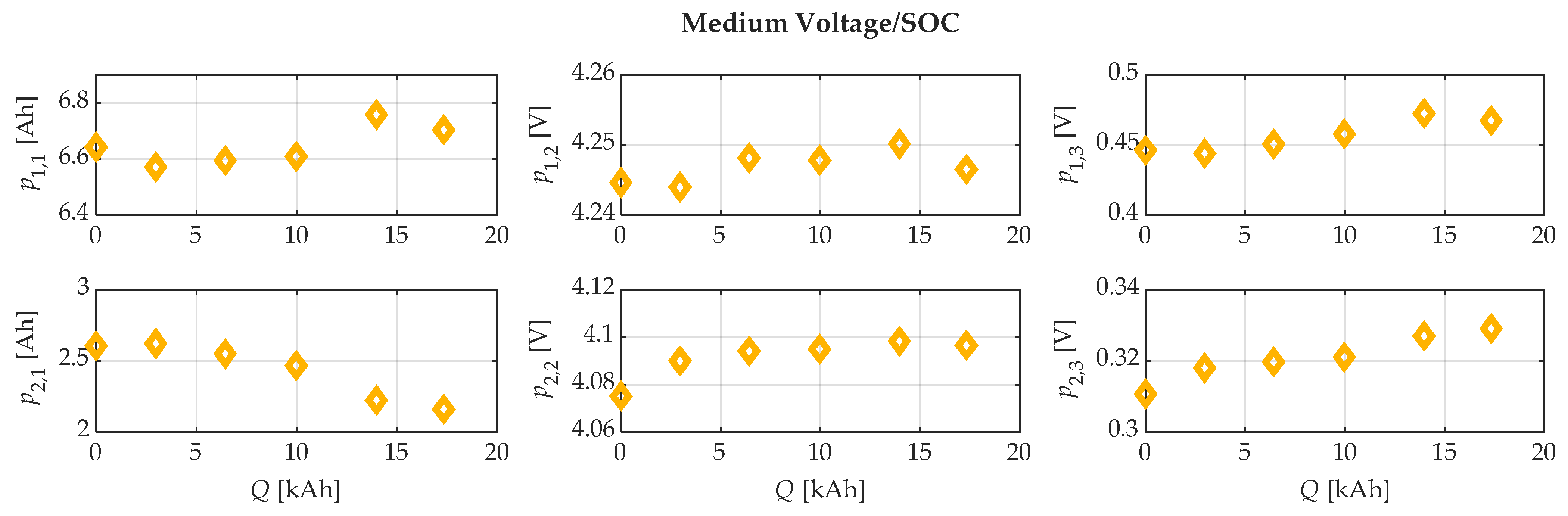
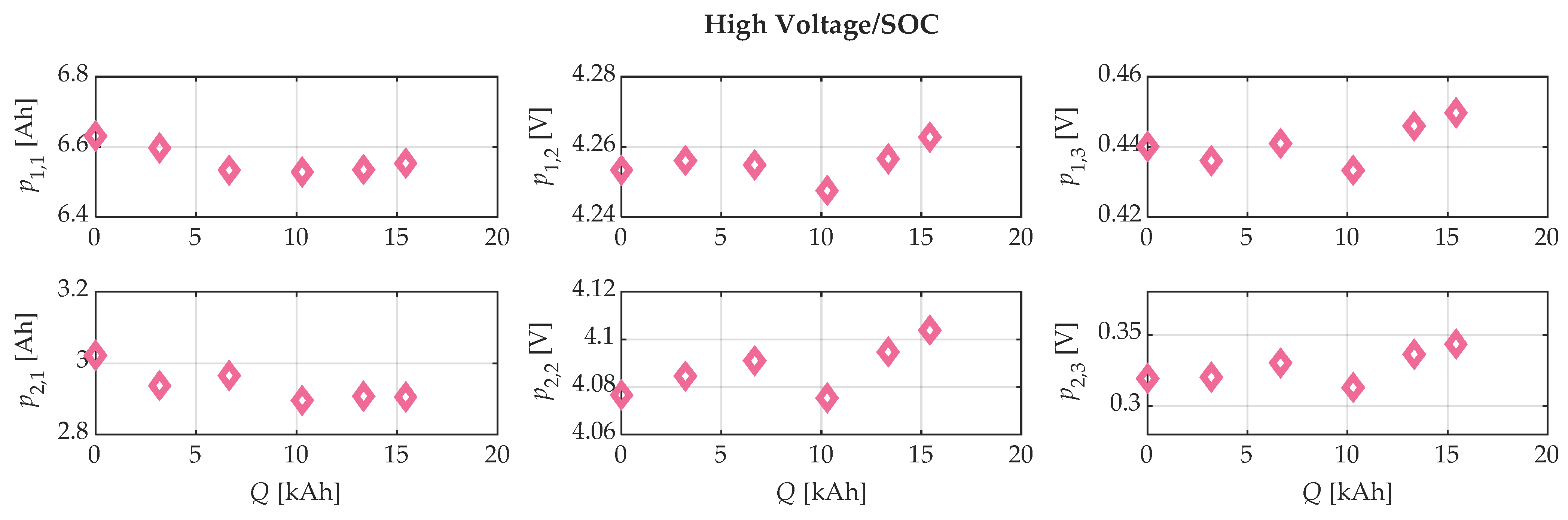
The next step was to analyze how the parameters of the proposed model vary as a function of the cycling level, Q, with the aim of modeling their behavior through additional analytical functions. Figure 6, Figure 7, and Figure 8 show the trends of the six parameters for the battery cycled in the low, medium, and high voltage/SOC conditions, respectively.

From these trends, it is evident that p_1,2, p_1,3, p_2,2, and p_2,3 display similar behavior across all operating conditions. This suggests that these parameters may be correlated, potentially allowing a reduction in the number of independent parameters that vary with the cycling level.

Specifically, from an analytical standpoint, parameters p_1,1 and p_2,1 represent the maximum amplitude of the Gaussian functions along the vertical axis; therefore, they can be physically related to the battery capacity. Parameters p_1,2 and p_2,2, which determine the position of these maximum values, can be associated with the characteristic voltage levels of the battery. Finally, parameters p_1,3 and p_2,3, which control the spread along the horizontal axis, can be related to the width of the battery voltage range.

In particular, the sum of p_1,1 and p_2,1 is approximately equal to the actual battery capacity; the values of p_1,2 and p_2,2 are close to the maximum cutoff voltage of the battery, where the absolute state of charge reaches the battery capacity. Finally, the sum of p_1,3 and p_2,3 is approximately 1 V, which can be related to the voltage range over which the absolute state of charge, q, starts to increase more rapidly as a function of the OCV.

After several trials, it was found that for each voltage/SOC condition, by fixing all parameters except p_2,1 at their average values obtained from the previous fitting procedure, the remaining parameter alone is sufficient to capture the overall behavior. Specifically, the fitting process was repeated under this constraint, and a linear least-squares algorithm was employed, as the problem then becomes linear.

Table 2. Average value of the fixed parameters.

Voltage/SOC Condition	p1,1	p1,2	p1,3	p2,2	p2,3
Low	6.678	4.258	0.4421	4.089	0.3314
Medium	6.647	4.247	0.4566	4.092	0.3210
High	6.563	4.255	0.4410	4.088	0.3271

reports the average values of the parameters discussed above.

The results of these updated fitting procedures are presented in Figure 9, Figure 10 and Figure 11. As before, a good agreement is observed between the experimental data of the q–OCV curves and the corresponding model predictions across all voltage/SOC conditions and cycling levels. This agreement is further confirmed by R² values exceeding 0.9997, 0.9985, 0.9993 for the low, medium, and high voltage/SOC conditions, respectively, across all cycling levels.

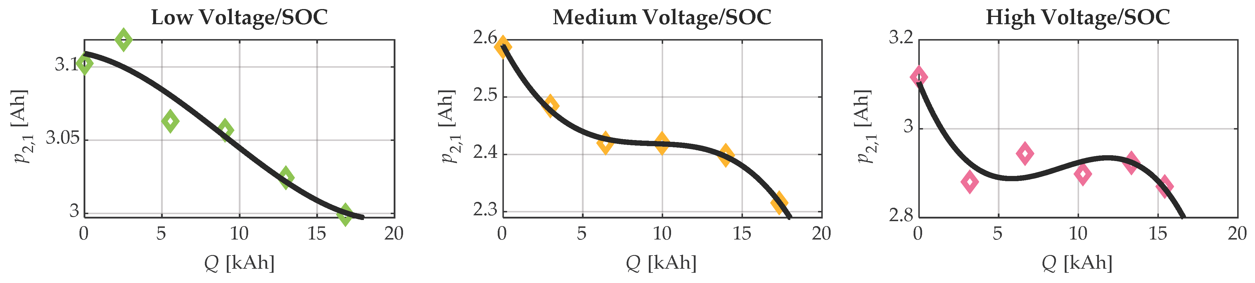
The only free parameter, p_2,1, in (3) is shown in Figure 12, where a well-defined trend can be observed for the three voltage/SOC conditions. To obtain a complete q–OCV model dependent on the cycling level, p_2,1 was modeled using the following analytical function:

$$p_{2,1}(Q)=z_1{Q}^3+z_2{Q}^2+z_{3}Q+z_4$$

(5)

The previously obtained values of p_2,1 were fitted to this function using a linear least-squares algorithm. The fitting results, also reported in Figure 12, show a good agreement between the measured values of p_2,1 and the corresponding analytical predictions. The coefficients of (5) are listed in

Table 3. Coefficients of (5).

Voltage/SOC Condition	z1 [Ah−2]	z2 [Ah−1]	z3	z4 [Ah]
Low	2.535 × 10–14	−6.833 × 10–10	−2.137 × 10–6	3.109
Medium	−1.920 × 10–13	5.438 × 10–9	−5.234 × 10–5	2.590
High	−4.296 × 10–13	1.139 × 10–8	−8.891 × 10–5	3.104

.

The fact that only parameter p_2,1, corresponding to one of the amplitude coefficients of the Gaussian functions, needs to vary with cycling level to accurately describe the degradation of the q–OCV curve suggests that the overall shape of the OCV curve remains substantially stable during cycle aging. In this framework, the variation in p_2,1, which can be physically related to battery capacity, captures the capacity fade associated with the vertical scaling of the curve.

4.2. Validation of the Model

According to the characterization procedure for the q–OCV model described in the previous section, its validation was carried out using the entire dataset. As an example, the results for three cases—selected from the dataset and not included in the characterization subset—are reported and compared with the experimental data in Figure 13, Figure 14 and Figure 15 for the low, medium, and high voltage/SOC operating conditions, respectively. From these figures, a good agreement can be observed between the estimated and measured OCV values across the different cycling levels and operating conditions.

It is worth noting that for each operating condition, the highest cycling level lies outside the range used for the characterization subset, thus providing an indication of the model’s capability to extrapolate and accurately predict the q–OCV curves beyond the characterization interval.

Furthermore, the R² was computed for all datasets. The resulting values—consistently above 0.9996, 0.9997, and 0.9981 for the low, medium, and high voltage/SOC conditions, respectively, across all cycling levels—further demonstrate the high accuracy of the proposed model.

4.3. Capacity and SOC Estimation

The proposed model can be used to estimate the actual battery capacity, C_bat,a,est, and state of charge, SOC_est, based on the knowledge of the experimental OCV value, OCV_exp, and the cycling level, Q, for each voltage/SOC condition.

In particular, the proposed q–OCV model can be directly applied to determine the estimated actual battery capacity, C_bat,a,est, by imposing the maximum cutoff voltage of 4.2 V in (3), i.e., C_bat,a,est = q(4.2 V). To estimate the actual state of charge, SOC_est, the measured OCV value, OCV_exp, is substituted into (3) to obtain the corresponding absolute state of charge, q_est, i.e., q_est = q(OCV_exp). Finally, SOC_est is computed using (2).

To evaluate the accuracy of the battery capacity and SOC estimations, the estimated values C_bat,a,est and SOC_est were compared with the corresponding experimental battery capacity, C_bat,a,exp, and state of charge, SOC_exp.

Specifically, the values of C_bat,a,exp were obtained by integrating the battery current during a full discharge using (1). Consequently, the values of SOC_exp were obtained through (2) using the experimental absolute state of charge, q_exp, and the actual battery capacity C_bat,a,exp. The following battery capacity and SOC estimation errors were evaluated:

$$\begin{array}{l}{e}_C={\displaystyle \frac{\left|C_{bat,a,est}-C_{bat,a,exp}\right|}{C_{bat,a,exp}}}\\ e_{\mathrm{SOC}}=\left|{\mathrm{SOC}}_{est}-\mathrm{SOC}\right|=\left|{\displaystyle \frac{q_{est}}{C_{bat,a,est}}}-{\displaystyle \frac{q_{exp}}{C_{bat,a,exp}}}\right|\end{array}$$

(6)

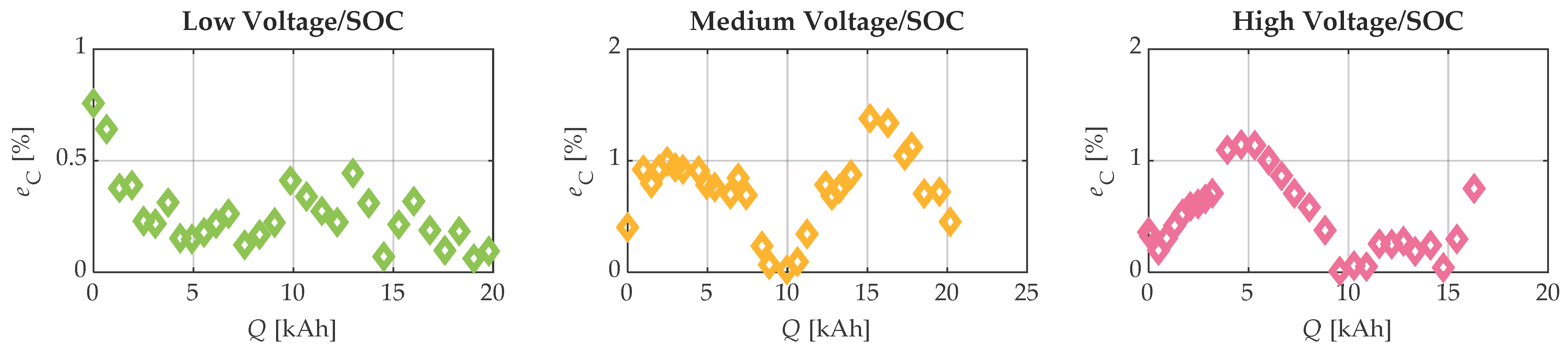
The percentage battery capacity estimation errors are reported in Figure 16 as a function of the cycling levels and for each voltage/SOC condition. The results show that the battery capacity estimation error is approximately below 0.7% for the low voltage/SOC condition, 1.4% for the medium voltage/SOC condition, and 1.2% for the high voltage/SOC condition.

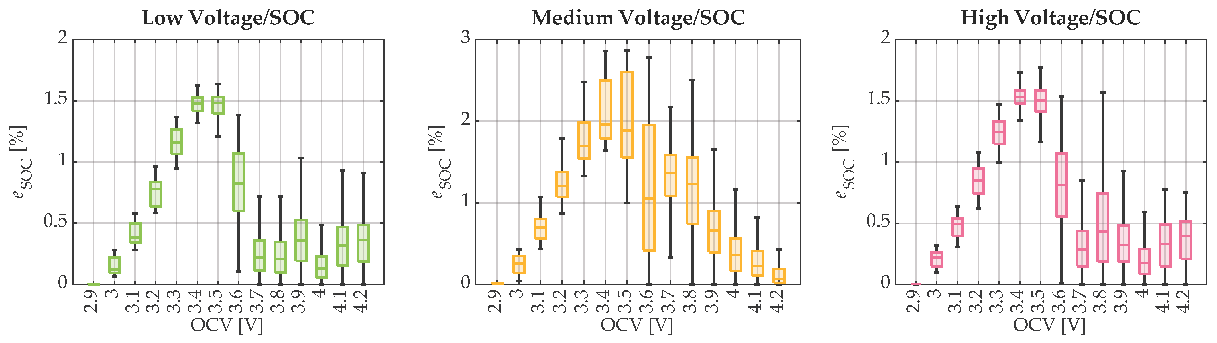
The percentage SOC estimation errors are represented by the boxplot in Figure 17 as a function of the OCV at different cycling levels and for each voltage/SOC condition. As can be observed, for the low voltage/SOC dataset, the median error remains below 1.5%, while the interquartile range is within 0.5%. For the medium voltage/SOC dataset, the median error remains below 2%, with an interquartile range of about 1.5%. For the high voltage/SOC dataset, the median error remains below 1.6%, and the interquartile range is approximately 0.5%.

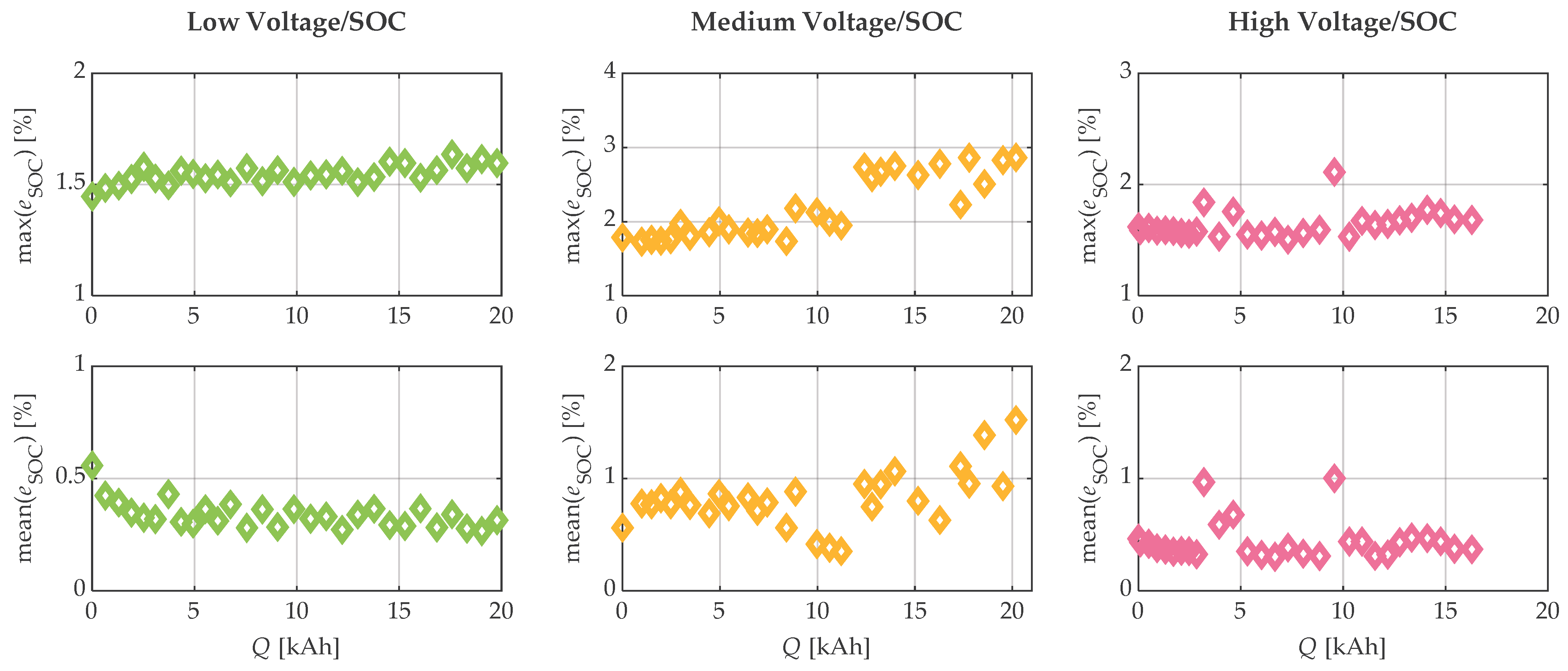
Specifically, both the mean and maximum percentage SOC estimation errors were evaluated over the entire q–OCV curve as a function of the cycling level and for each voltage/SOC condition, as reported in Figure 18. These results highlight the high accuracy of the proposed method. For the low voltage/SOC dataset, mean errors remain below approximately 0.5%, with maximum errors around 1.5%. For the medium voltage/SOC dataset, mean errors are below about 1.5%, with maximum errors ranging between 2% and 3%. For the high voltage/SOC dataset, mean errors stay below approximately 1%, while maximum errors range between 1.5% and 2%.

It is worth highlighting that from the experimental q–OCV curves, a smooth trend in capacity reduction can be observed across all voltage/SOC conditions, indicating that the so-called knee point in the capacity fade was not reached. This point typically marks the transition to accelerated degradation. In this context, the proposed modeling approach is expected to remain valid within the pre-knee region, where the degradation trend is relatively smooth and well-behaved. Beyond this point, i.e., after the knee, additional degradation mechanisms may become dominant, potentially leading to nonlinearities or threshold-like behavior that are not explicitly captured by the present model.

A detailed investigation of the model validity in the post-knee region, as well as the identification of possible critical points or threshold effects, represents an interesting direction for future work.

5. Conclusions

In this study, the q–OCV model introduced in [40], which relies on a six-parameter generalized Gaussian formulation and was previously evaluated under cycle aging conditions only within a restricted SOC range, was further developed to examine cycle aging effects in the same battery type over a broader operating window, encompassing low, medium, and high voltage/SOC conditions.

The six parameters of the q–OCV model were initially identified using a nonlinear least-squares fitting procedure applied to a selected subset of the experimental data for different cycling levels and each voltage/SOC condition. Based on the resulting trends of these six parameters, an interdependency among them was observed, which led to fixing five parameters at their average values obtained from the initial fitting. In this way, a second fitting procedure was performed using a linear least-squares algorithm, since the resulting problem becomes linear with respect to the single remaining free parameter. Consequently, the evolution of this free parameter was modeled as a function of the cycling level using a polynomial function.

Finally, the model was validated over the entire experimental dataset for each voltage/SOC condition, allowing direct estimation of both the actual battery capacity and SOC without the need for extensive look-up tables or numerical inversion of the classical OCV–SOC relationship, thus reducing the need for large memory resources and computational complexity. These features make the model particularly attractive for real-time onboard BMS applications. Specifically, the battery capacity was estimated with a maximum error of 1.2%, while SOC estimation showed a maximum mean error of 1.5% across all experimental data.

Although the present analysis focused on LCO batteries, we expect the model to remain applicable to batteries employing cobalt-based layered cathodes, such as nickel manganese cobalt oxide and nickel cobalt aluminum oxide, which exhibit similar OCV characteristics. Nevertheless, future work could investigate the applicability of the same approach to different battery chemistries under identical testing conditions, in order to assess whether the model remains valid or requires adaptation. This may be the case for chemistries such as lithium iron phosphate, where the presence of a pronounced voltage plateau in the OCV curve could require the inclusion of additional terms or a modified formulation to accurately capture the behavior.

Furthermore, additional investigation of the model validity in the post-knee region of capacity fade, as well as the impact of temperature on cycle aging, could also be considered as part of future work.