Bayesian Gaussian Mixture Model Classifier for Fault Detection in Induction Motors Using Start-Up Current Analysis

Abstract

Induction motors constitute a major share of industrial drives, making reliable fault detection essential for maintaining operational continuity. This work develops a Bayesian classifier for identifying rotor-bar damage using start-up current measurements represented in the frequency domain. The spectra are modelled as smooth functional curves using a hierarchical B-spline formulation, and posterior sampling provides a generative mechanism for augmenting scarce labelled data. Classification is performed using a Bayesian Gaussian mixture model, where each prediction is obtained by averaging over thousands of posterior samples, yielding stable and interpretable probability estimates. In experimental evaluation, the proposed approach achieves consistent separation between healthy and faulty motors across repeated training runs, correctly identifying all test cases in the binary classification setting and exhibiting more stable probability estimates than logistic and soft-max regression under limited labelled data. The model additionally signals atypical responses for unmodelled faults, indicating potential for anomaly detection. These findings highlight the suitability of Bayesian functional modelling as a reliable tool for induction motor condition monitoring.

1. Introduction

Induction motors are essential in industrial and commercial applications due to their robustness, efficiency, and versatility. Their continuous operation can lead to faults, requiring early detection to extend motor lifespan and prevent severe damage and costly repairs. Traditional diagnostic methods often involve downtime for maintenance checks, but statistical approaches expedite fault detection, enabling efficient analysis of large datasets and ensuring reliable operation.

Faults in induction motors are classified as electrical or mechanical. Electrical faults, such as stator winding failures and broken rotor bars, arise from issues like insulation breakdown, unbalanced power supply, or mechanical stresses, leading to problems such as localized heating, vibration, and torque pulsations [1]. Mechanical faults, including bearing failures and rotor misalignment, are caused by improper installation, vibration, or lubrication degradation, resulting in increased wear and premature failure [2]. In this work, we focus on the analysis of broken rotor bars, considered among others in [3].

Diagnostic approaches for induction motors exploit a broad range of measured quantities and processing techniques. Depending on the type of fault, information can be extracted from electrical, magnetic, mechanical, or acoustic signals. For example, frequency-domain analysis of stator quantities has been used to identify inter-turn faults [4], while acoustic signatures have been shown to be sensitive to rotor-related defects [5,6]. Motor Current Signature Analysis (MCSA) remains one of the most established tools, as characteristic sidebands in the current spectrum can indicate bearing wear, air-gap eccentricity, or rotor asymmetries [7]. More recently, multi-sensor schemes combining several data sources have been proposed, often together with dimensionality reduction techniques such as principal component analysis to improve interpretability and reduce noise [8,9].

A large portion of the literature concentrates on steady-state operation, where the signals are easier to interpret and to acquire in a repeatable way [10,11]. However, the start-up phase contains rich transient phenomena that are directly affected by rotor asymmetries and other faults [12,13]. These transients are non-stationary and typically analysed using time–frequency tools, including wavelet-based methods [14,15,16] or spectrograms [17], which highlight the evolution of spectral components during acceleration. Recent studies have demonstrated that transient and start-up regimes can be successfully exploited for fault detection under non-stationary operating conditions, including fluctuating loads and variable-speed operation [3,17,18]. In addition to current-based approaches, stray-flux measurements combined with modern machine learning techniques have been shown to enable multi-fault diagnosis under low-frequency load oscillations [19].

In this work, we follow a different strategy: after appropriate filtering and band selection, we represent the start-up current in the frequency domain and treat the resulting magnitude spectra as functional objects defined on a common frequency grid.

There is also an active line of research that applies machine learning and deep learning to motor diagnostics. Techniques based on handcrafted features combined with classical classifiers, as well as convolutional neural networks operating directly on raw or transformed signals, have been explored in the literature [20]. While such methods can achieve high accuracy, they typically rely on large labelled datasets and careful hyperparameter tuning. On the other end of the spectrum, physics-based models such as finite element simulations [21,21] can be used to generate synthetic signals under various fault conditions, but they require substantial modelling effort and are less flexible when the real system deviates from the assumed model. Recent review studies confirm that, despite rapid progress in machine learning-based diagnostics, current-signature approaches remain attractive due to their non-intrusive nature, but they often lack systematic treatment of uncertainty, particularly in transient regimes [22].

Probabilistic methods, and Bayesian models in particular, offer a complementary perspective that is attractive in diagnostic problems where datasets are small, heterogeneous, or costly to obtain. In this framework, uncertainty in parameters and predictions is treated explicitly, which is important when making maintenance decisions. Bayesian techniques have been successfully applied to several prognostic and diagnostic tasks, including fault identification in diesel engines [23] and remaining useful life estimation from sensor histories [24]. Gaussian mixture models (GMMs) are especially appealing in this context because they naturally provide probabilistic class assignments and can approximate complex distributions [25,26]. Their variants have been combined with neural architectures for induction motor diagnostics [27,28], and Bayesian versions of GMMs have been used for cable fault location in settings where the signals have a relatively homogeneous character [29].

Despite these advances, the literature still lacks probabilistic, uncertainty-aware frameworks that operate directly on frequency-domain representations of start-up currents while explicitly addressing data scarcity and variability across operating conditions. Most existing transient-based approaches rely on deterministic feature extraction or require large labelled datasets, limiting their applicability in practical diagnostic scenarios. The present work aims to fill this gap by combining Bayesian functional modelling of start-up current spectra with a Gaussian mixture classifier, yielding stable probabilistic predictions and principled uncertainty quantification even under limited training data.

In this study, we combine a Bayesian functional representation of start-up currents with a Bayesian GMM classifier. The start-up current of each motor is first transformed to the frequency domain and modelled using B-spline bases within a hierarchical Bayesian framework. The resulting functional models are then used to generate synthetic spectra that augment the limited real data and serve as inputs to a Bayesian GMM classifier operating either in a binary or a three-class setting. Compared to our previous work [30], which focused on a preliminary version of this approach, we provide an extended formulation, a more systematic evaluation, and a broader comparison with classical methods. The specific contributions of this paper are as follows:

• We construct a Bayesian functional model based on B-splines that captures both measurement noise and parameter uncertainty in the frequency-domain representation of start-up currents;
• We develop binary and three-class Bayesian GMM classifiers that distinguish between healthy motors and motors with one or two broken rotor bars;
• We investigate the behaviour of the classifier under a non-modelled fault (a broken end ring) to illustrate its potential for anomaly indication;
• We compare the proposed Bayesian classifier with classical probabilistic models such as logistic and soft-max regression, using identical input representations.

The remainder of this paper is structured as follows: Section 2 describes the experimental setup and the preprocessing applied to the start-up current measurements. Section 3 presents the Bayesian methodology, including the functional representation of the spectra, the hierarchical generative model, and the construction of the mixture-based classifier. Section 4 reports the empirical evaluation, comparing the proposed approach with classical alternatives and examining its behaviour in the presence of unmodelled faults. Section 5 discusses the implications, practical considerations, and limitations of the proposed framework. Section 6 concludes the paper and outlines directions for future research.

2. Materials

The experiments were designed to examine how controlled rotor asymmetries influence the start-up behaviour of induction motors, with particular emphasis on obtaining transient current profiles suitable for statistical modelling. To ensure that the resulting data would reflect comparable operating conditions across all examined fault scenarios, the experimental setup was configured to provide (i) reproducible mechanical loading, (ii) sufficiently long acceleration intervals, and (iii) a consistent electrical supply environment. These considerations guided the choice of motors, the method of introducing rotor faults, and the configuration of the drive assembly.

2.1. Considered System

All tests were performed on four identical squirrel-cage induction motors of type Sg 100L–4A (Indukta, Cantoni Group—Cieszyn, Poland) [31]. Each machine was rated for three-phase 230 V $\Delta$/400 V Y operation with a nominal output power of 2.2 kW and corresponding rated currents of 8.4 A and 4.8 A, respectively. The motors operate at a rated frequency of 50 Hz, provide a nominal speed of 1425 rpm, and have a power factor of $cos\phi =0.80$. They are designed for continuous duty (S1), feature class F insulation, deliver an efficiency of $\eta =82.0\%$, and comply with ingress protection class IP55. The use of identical machines ensured that any observed variation in electrical signatures could be attributed to the imposed rotor conditions rather than to unit-to-unit differences.

To emulate typical rotor-cage degradation patterns, controlled modifications were introduced to selected rotors. One machine was kept in its original state and served as the reference unit. In the second motor, a local discontinuity was created in a single cage bar to reproduce the characteristics of a classical one-bar fracture by drilling a through-hole in the aluminium rotor bar, with the hole diameter equal to the bar width, thus fully interrupting the bar’s continuity. A third rotor was altered in an analogous manner but with two bars affected using the same drilling procedure applied to two separate cage bars, representing a more advanced stage of the same fault mechanism. In the fourth motor, a partial cut was made in one of the end rings by mechanically cutting the ring on one side, imposing an interruption of current redistribution within the cage and representing a qualitatively different form of asymmetry. Although the mechanical integrity of all motors remained intact, these electrical alterations changed the electromagnetic torque production and, thus, the current response during run-up.

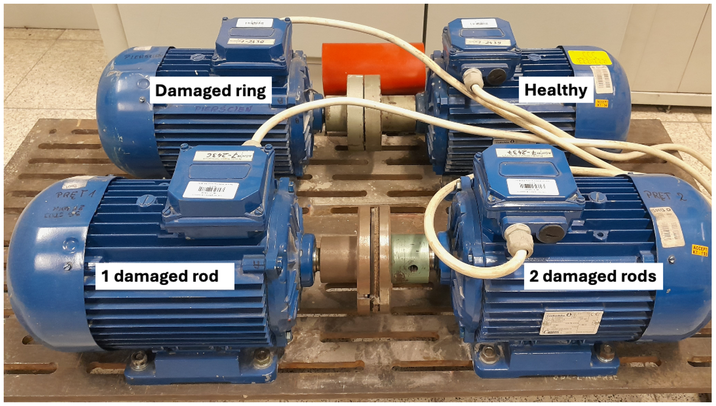
During testing, the motors were mechanically coupled in pairs to form a drive-load arrangement. This configuration increased the effective moment of inertia seen by the supplied motor, which, in turn, lengthened the acceleration period and provided a richer transient for analysis. Additionally, the supply voltage was lowered from the nominal value, further extending the duration of the start-up interval while keeping thermal loading modest. Both measures ensured that the transient currents captured under different rotor conditions were sufficiently long and structurally comparable to allow functional modelling. An overview of the mechanical arrangement and motor placement is shown in Figure 1.

2.2. Measurement Setup and Signal Characteristics

The electrical signals were acquired using a multi-channel data acquisition system equipped with LEM current and voltage transducers. Specifically, an MCC USB-1608FS-Plus [33] data acquisition card with simultaneous analogue inputs and 16-bit resolution was used for signal acquisition. Voltage measurements were performed using LEM LV25-P [34] voltage transducers, while current measurements were carried out using LEM LA 55-P [35] current transducers. The transducers were connected directly to the data acquisition card without an additional external analogue conditioning stage. To improve the effective sensitivity of the current measurements, the measured conductor was wound five turns around the current transducer, increasing the output signal amplitude proportionally.

The sampling rate was set to 1150 Hz, which provided adequate temporal resolution for capturing low-frequency components relevant to rotor asymmetry while maintaining a comfortable margin above the Nyquist limit for the analysis bandwidth considered. Since the diagnostic focus in this study lies below 50 Hz, the chosen sampling frequency ensured that harmonic content associated with the supply and with rotor-speed evolution could be captured without aliasing. It also allowed us to verify, by inspection of the raw spectra, that the most informative features for distinguishing fault types indeed occurred in this sub-50 Hz region, consistent with earlier observations on motors with cage irregularities [36].

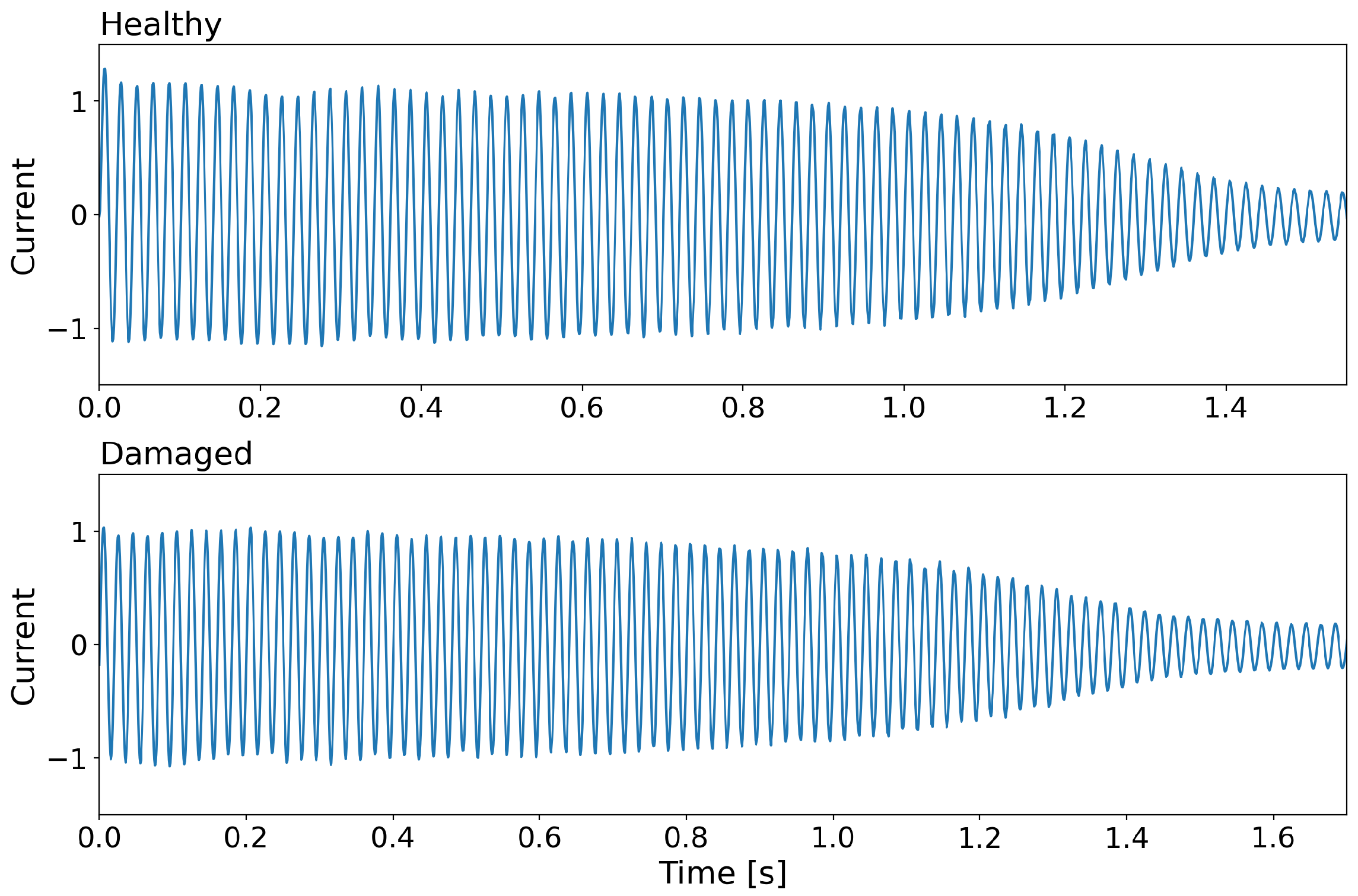
The recorded start-up currents exhibited substantial variation in both amplitude and duration due to the combined effects of different fault conditions and intentionally modified supply voltages. As a result, the time-domain waveforms of motors with and without rotor asymmetries often appeared visually similar, and the direct comparison of raw signals was not sufficient to reliably highlight the underlying differences. Representative unprocessed start-up currents illustrating this variability are displayed in Figure 2. More discriminatory behaviour became apparent when examining how spectral energy evolves during start-up. The resulting magnitude spectra for representative healthy and faulty cases are compared in Figure 3. Time–frequency representations revealed that fault-induced components manifest primarily in the lower-frequency region, and that their prominence varies across motors and test conditions.

To obtain a common representation suitable for further statistical analysis, the signals were filtered to suppress the dominant 50 Hz supply component and then transformed into the frequency domain. Working with magnitude spectra mitigated issues associated with varying signal lengths and enabled a more direct comparison across tests. These spectra serve as the basis for the functional modelling strategy introduced in the next section.

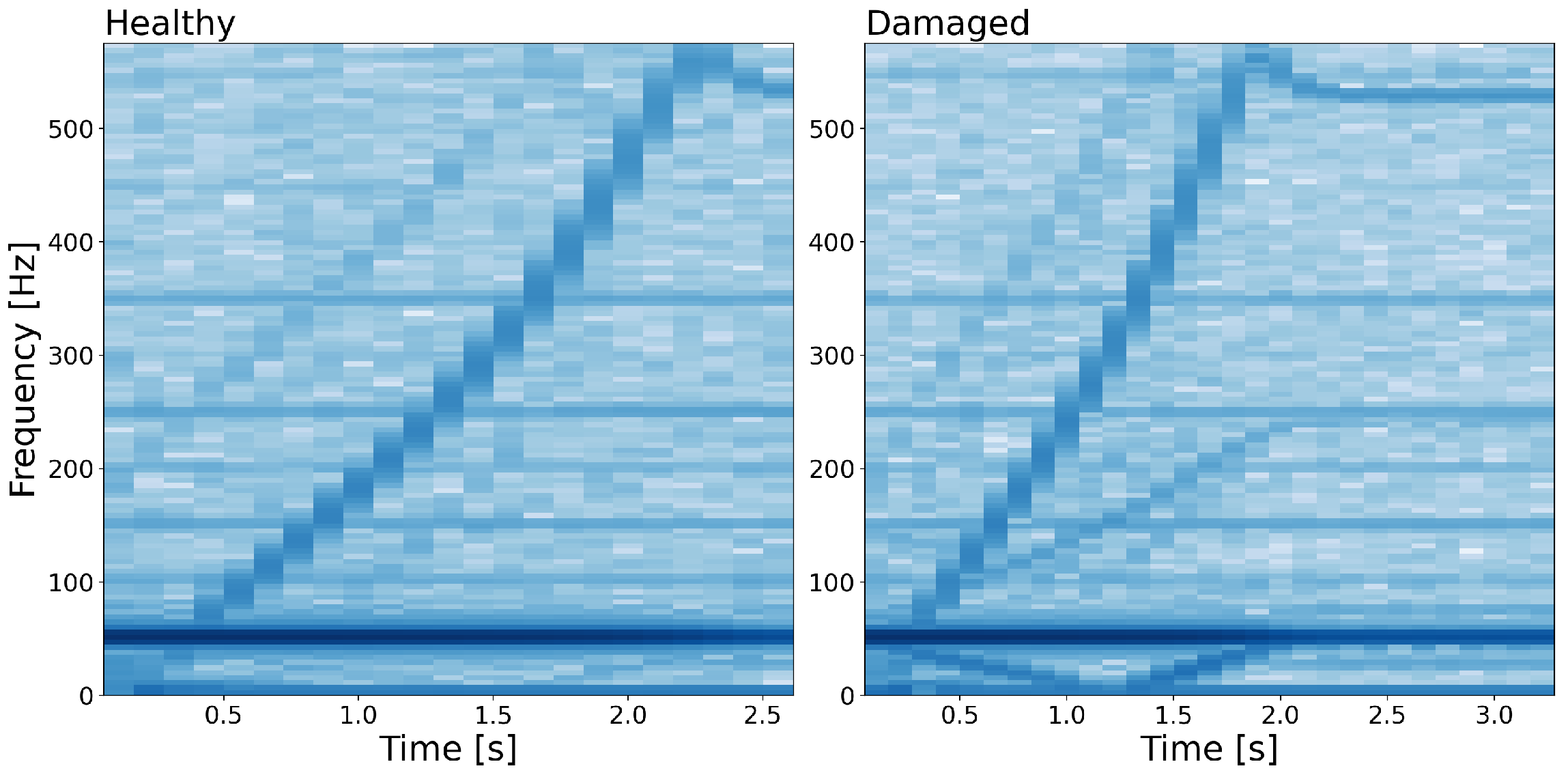
The classical approach of using rolling root mean squared is not efficient for diagnostics because of information loss. The frequency domain allowed us to eliminate the problem of varying time. Investigating spectrograms of currents showed that the lower-frequency band tends to contain some components that are much more prominent in signals from damaged motors (Figure 3).

The spectrograms of the currents in Figure 3 indicate that the differences between a damaged and healthy motor appear for frequencies below 50 Hz. In particular, the low-frequency band contains components associated with electromagnetic asymmetry introduced by rotor cage faults, which are clearly visible during the start-up transient. In contrast, higher-frequency components predominantly follow the instantaneous rotational speed and its harmonics, forming diagonal structures in the spectrogram that primarily reflect mechanical acceleration rather than fault-specific electrical phenomena. To remove the 50 Hz band, which is the voltage supply frequency and at the same time dominates the spectrum, we used a notch filter, designed in Filterbuilder from Matlab/Simulink 2025a. The filter was constructed as a 6th-order system using the SOS Direct Form II implementation. We did not apply any low-pass filtering, as we only analysed the spectrum for frequencies less than 50 Hz.

Restricting the analysis to the sub-50 Hz range significantly improves the comparability of experiments performed under different start-up conditions and supply voltages, as this band is much less sensitive to variations in rotational speed. While higher-order harmonic components above 50 Hz may exhibit fault-related features under steady-state or specific load conditions, during start-up they are strongly speed-dependent and, therefore, hinder consistent alignment and comparison across experiments. Moreover, the results obtained using the 0–50 Hz band already provide high discriminability between healthy and damaged motors, making the inclusion of higher-frequency components unnecessary for the objectives of this study.

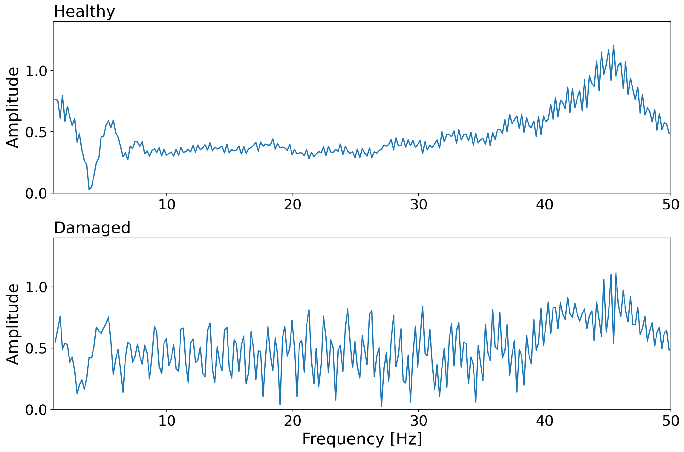
An example of the filtered signals for healthy and damaged motors is shown in Figure 4. Those frequency responses (0–50 Hz) are the basis of our algorithm.

2.3. Computational Setup

We employed Hamiltonian Monte Carlo (HMC) for Bayesian computation. HMC is a type of Markov Chain Monte Carlo (MCMC) method, which generates samples in such a way that the limiting distribution of the samples converges to the desired probability distribution. This is especially useful for Bayesian computation, as sampling from the posterior distribution is challenging. With the generated samples, we can estimate the expected values of desired functions of random variables, allowing us to answer a wide range of statistical questions. Samples are generated by taking values of appropriate Markov Chains, whose stationary distribution is the posterior. The practice of computation usually uses four individually generated chains of 1000 samples each (usually, 2000 are computed, and the first half are discarded as being part of a ‘warm up’). The current state-of-the-art software for HMC is Stan [37], which we utilized.

3. Methods

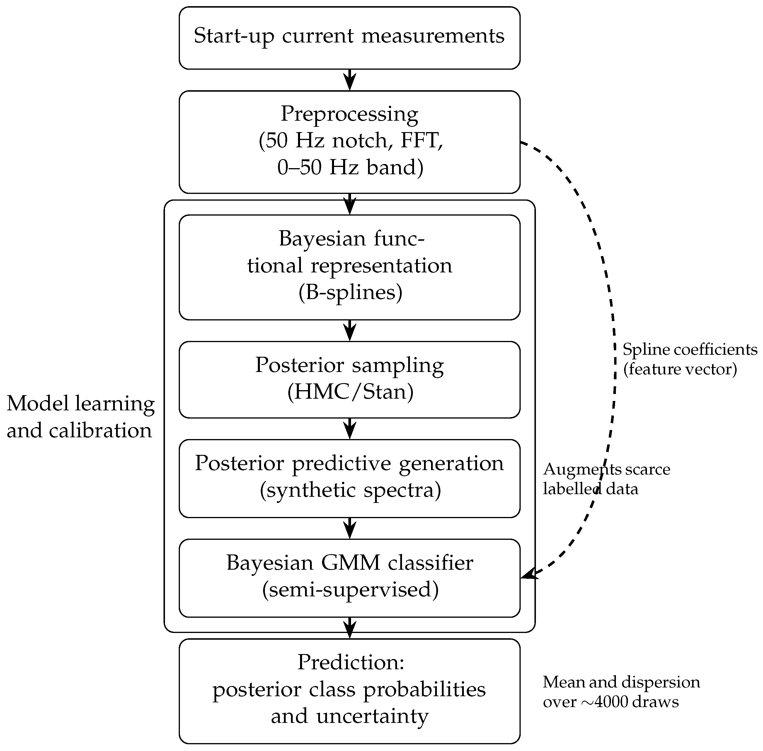
The methods used in this work combine functional modelling of the start-up current spectra with Bayesian classification techniques tailored to limited and partially labelled data. We begin by constructing a compact spline-based representation of each spectrum, which enables consistent comparison across signals of varying length and amplitude. A semi-supervised Gaussian mixture model is then formulated on this functional representation, providing class probability estimates by averaging over thousands of posterior parameter samples. The final part of this section examines the computational reliability of this inference process using simulation-based calibration. A high-level overview of the proposed methodology and data flow is provided in Figure 5.

3.1. Functional Representation of Frequency-Domain Data

The start-up currents collected in the experiments vary considerably in duration and scale, and these differences carry no diagnostic meaning on their own—they arise primarily from supply conditions and the increased mechanical inertia of the test stand. For subsequent statistical modelling, it is therefore advantageous to work with a representation that places all signals on a common domain while retaining the spectral characteristics that distinguish healthy behaviour from rotor-cage defects. The magnitude spectra obtained after filtering and Fourier transformation satisfy this requirement: they are smooth functions defined on a fixed frequency interval, and they compress the essential information into a form that can be compared across trials. Representative examples of these spectra for healthy and faulty cases are shown in Figure 4.

To formalize this representation, each spectrum is approximated by an expansion in a low-dimensional family of basis functions. Among the possible choices, B-splines offer a suitable compromise between flexibility and smoothness, allowing broad spectral trends to be captured without introducing artificial oscillations. Let ${\left\{{\varphi }_k\left(f\right)\right\}}_{k=1}^K$ denote such a set of spline functions defined over the analysed frequency range. The spectrum of a given signal is represented as

$$\mu \left(f\right)=\sum _{k=1}^K{\beta }_k{\varphi }_k\left(f\right),$$

where the coefficients ${\beta }_k$ determine the overall shape of the curve.

In practice, spectra are observed only at discrete frequency points $\left\{f_n\right\}$, and the measurements deviate from the smooth functional representation due to residual noise and interpolation effects. To account for these discrepancies, the measured values $Y_n$ are modelled as

$$Y_n\mid \beta ,\sigma \sim \mathrm{Normal}\left(\mu \left(f_n\right),\sigma \right),$$

with $\sigma$ describing the variability not explained by the spline expansion. The coefficients ${\beta }_k$ are treated as unknown parameters. Independent Gaussian priors,

$${\beta }_k\sim \mathrm{Normal}(0,1),$$

provide regularization and prevent overfitting in regions where the data offer limited support. An exponential prior,

$$\sigma \sim \mathrm{Exponential}\left(1\right),$$

is used to encode the assumption that the spectra are smooth and that the residual noise should remain small unless indicated otherwise. Posterior inference is carried out using Hamiltonian Monte Carlo, which produces samples from the joint distribution of $(\beta ,\sigma )$ and enables uncertainty quantification for the reconstructed curves. A closely related Bayesian spline-based generative formulation was previously introduced in the context of drone rotor diagnostics [38]. That work demonstrated that hierarchical spline representations, combined with probabilistic mixture modelling, can provide robust class structure even under limited availability of labelled training data. The present study adapts these principles to the frequency-domain representation of induction motor start-up currents, where data scarcity and strong variability similarly motivate a generative Bayesian approach.

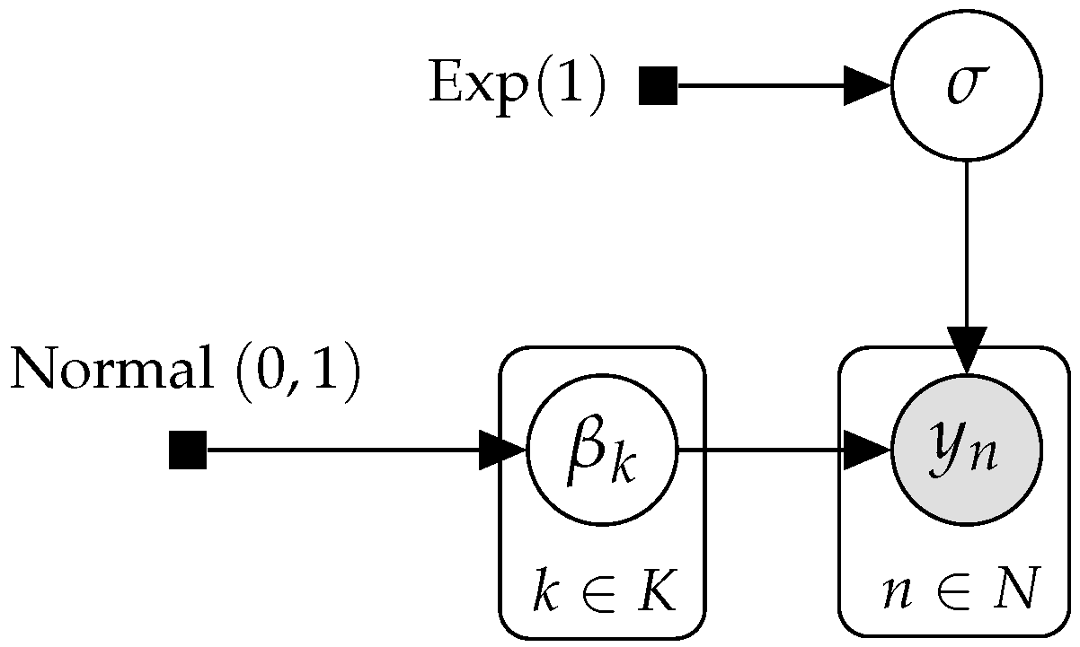
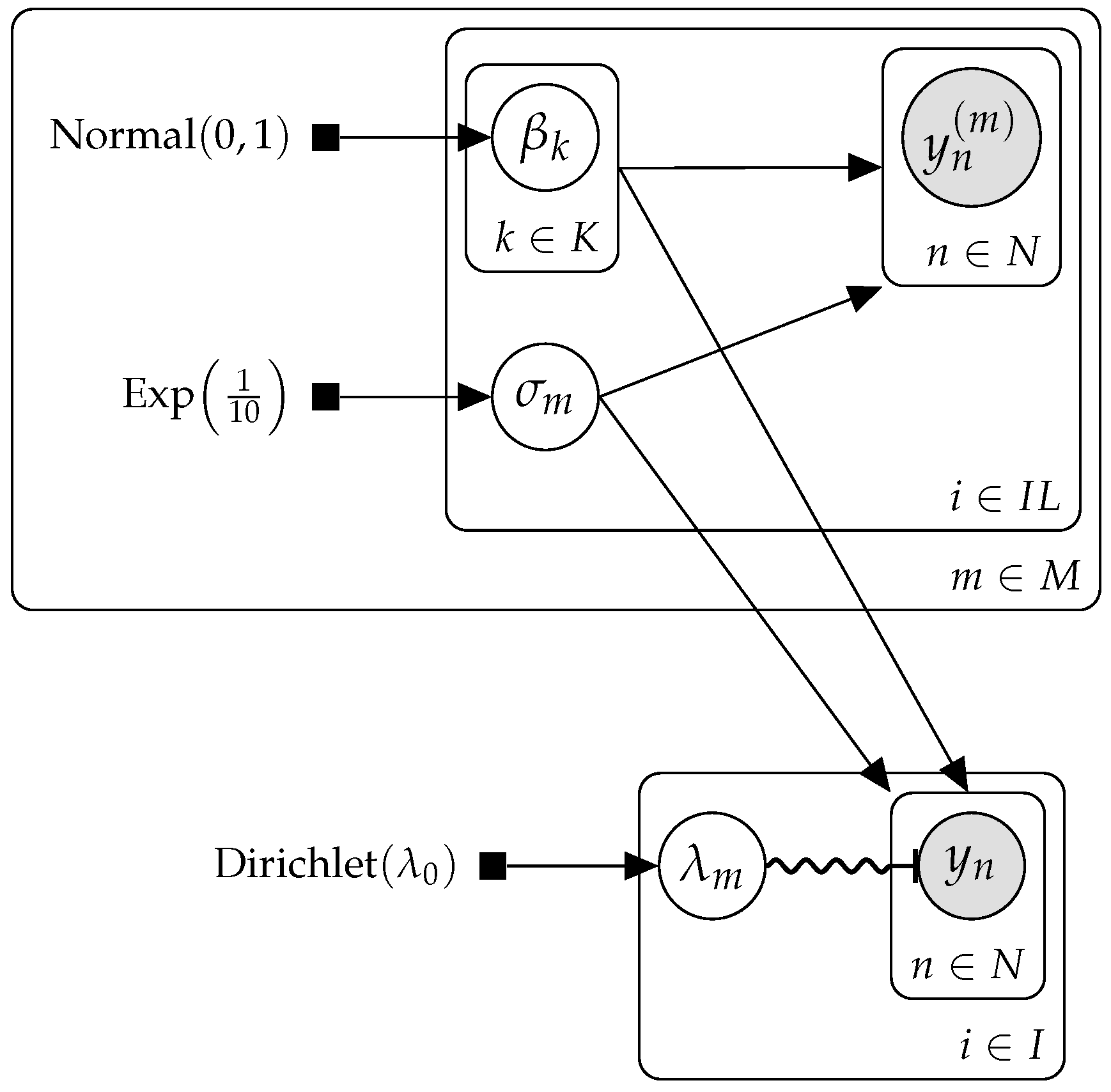
Figure 6 summarizes the hierarchical structure of the spline-based model in graphical form. The diagram highlights the separation between the latent coefficients that determine the smooth functional shape and the observational layer in which the measured spectral values are modelled with a shared noise scale. Although compact, this representation clarifies how uncertainty is propagated from the basis expansion to the reconstructed spectra, as well as how the likelihood links the functional model to the discrete frequency-domain observations.

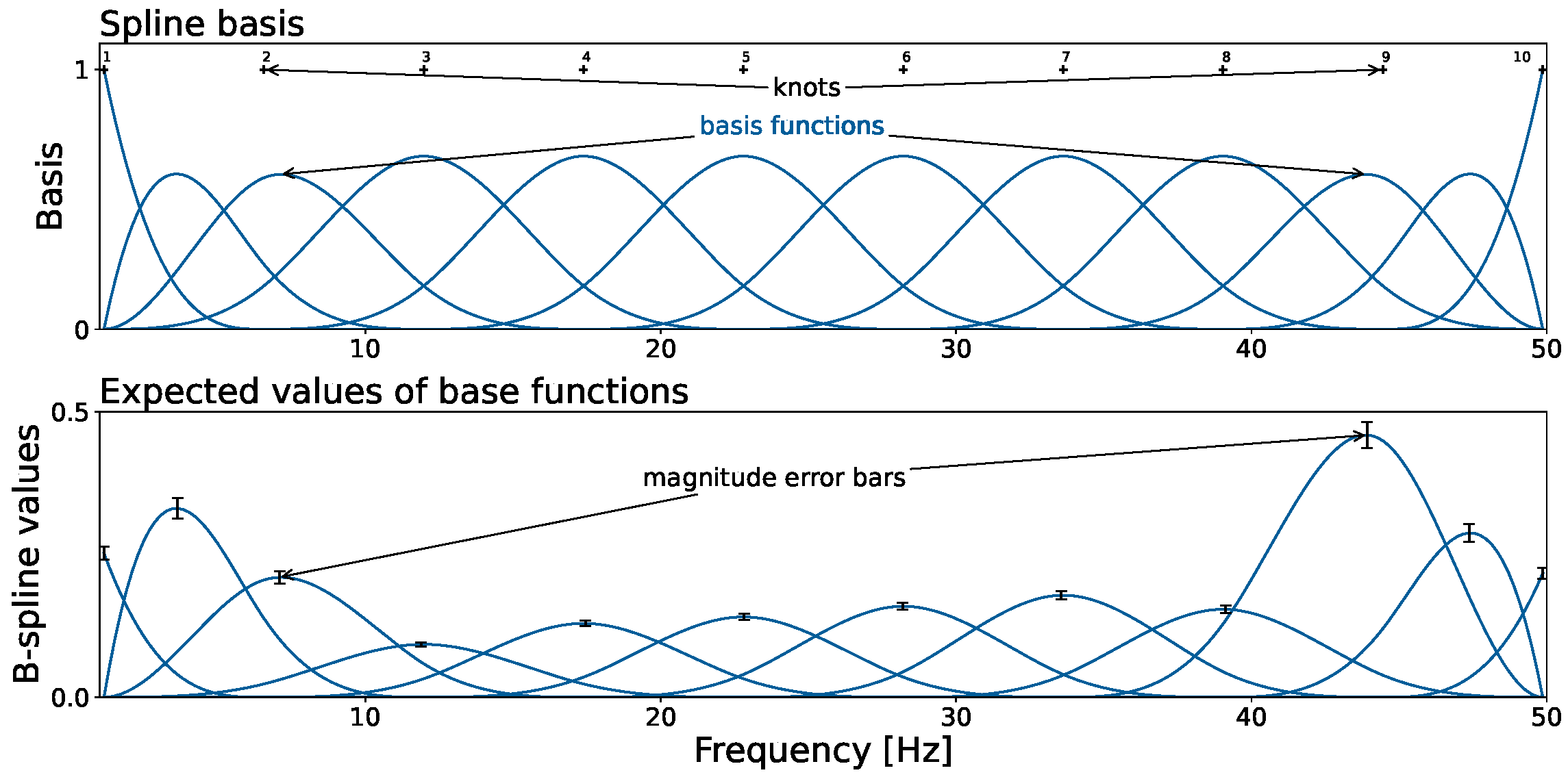
Figure 7 illustrates the chosen spline basis and the posterior mean curves obtained for one of the damaged classes.

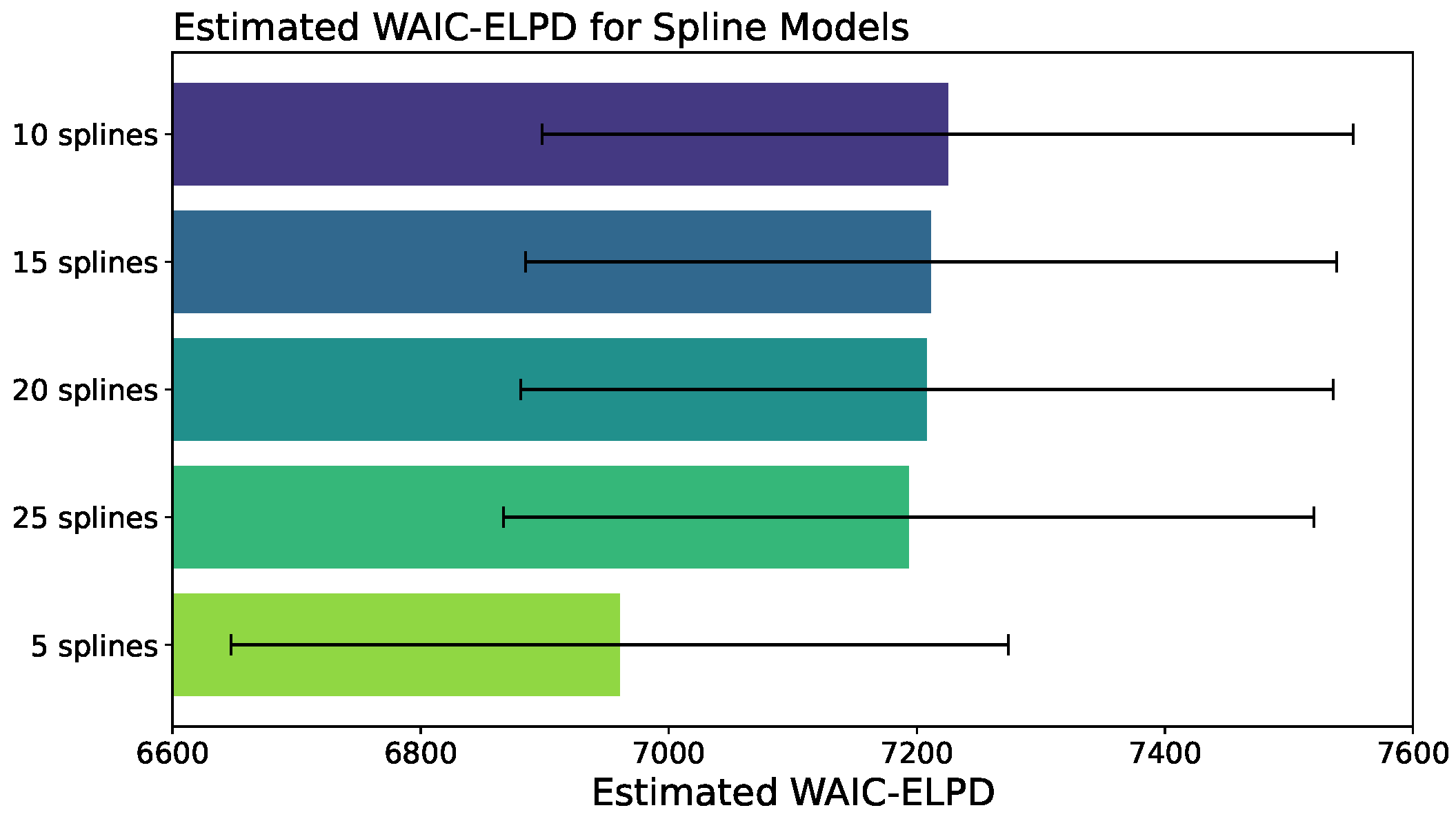
The number of basis functions K determines the balance between flexibility and noise suppression. If too few are used, the model cannot reproduce characteristic spectral features associated with cage faults; if too many are included, the representation becomes overly sensitive to noise. To identify a suitable basis dimension, models with different values of K were compared using predictive accuracy criteria and stability assessments across repeated runs. A basis of ten splines achieved a favourable accuracy–complexity trade-off, as illustrated in Figure 8. This configuration was therefore adopted for all subsequent analyses.

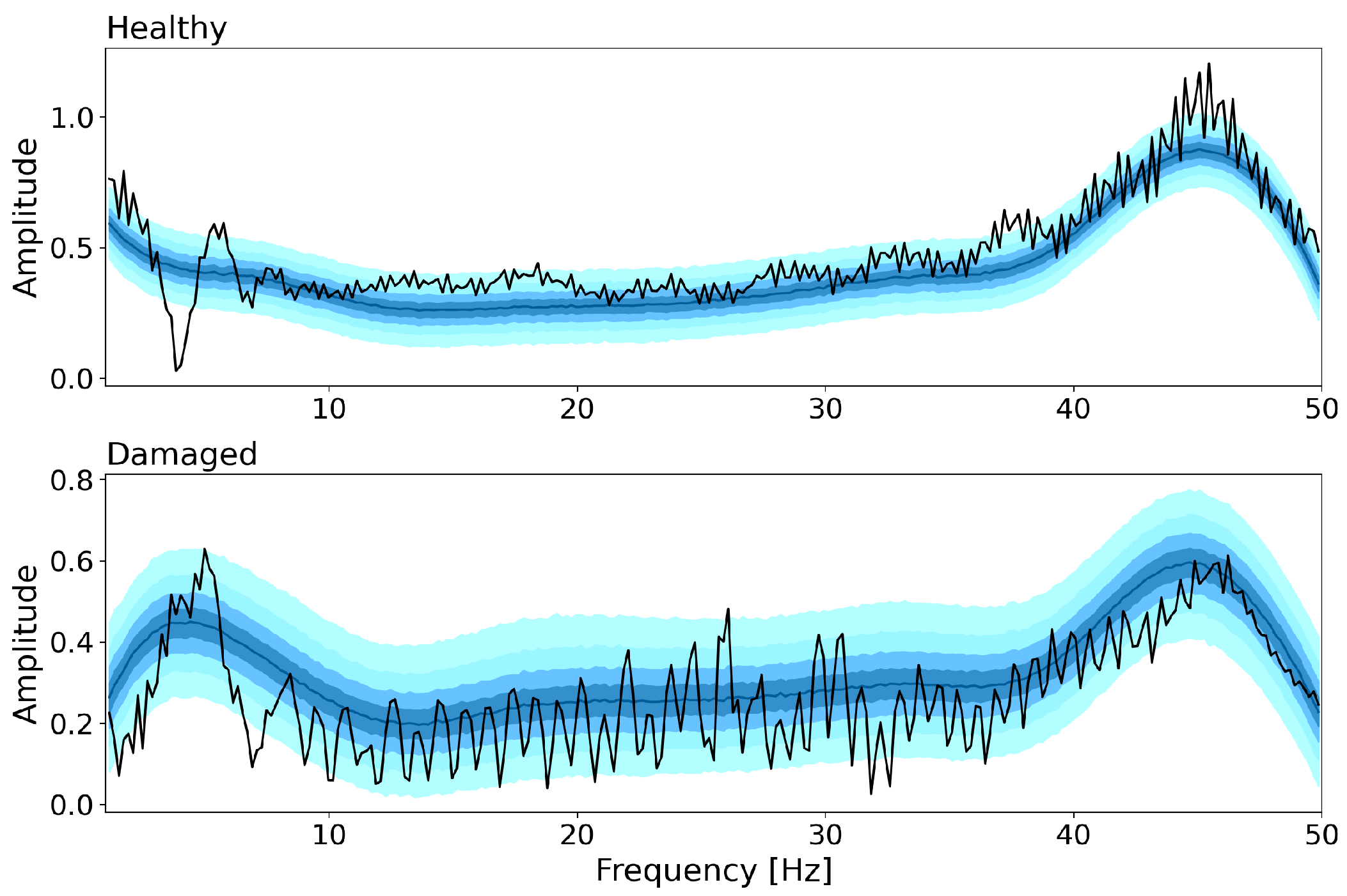
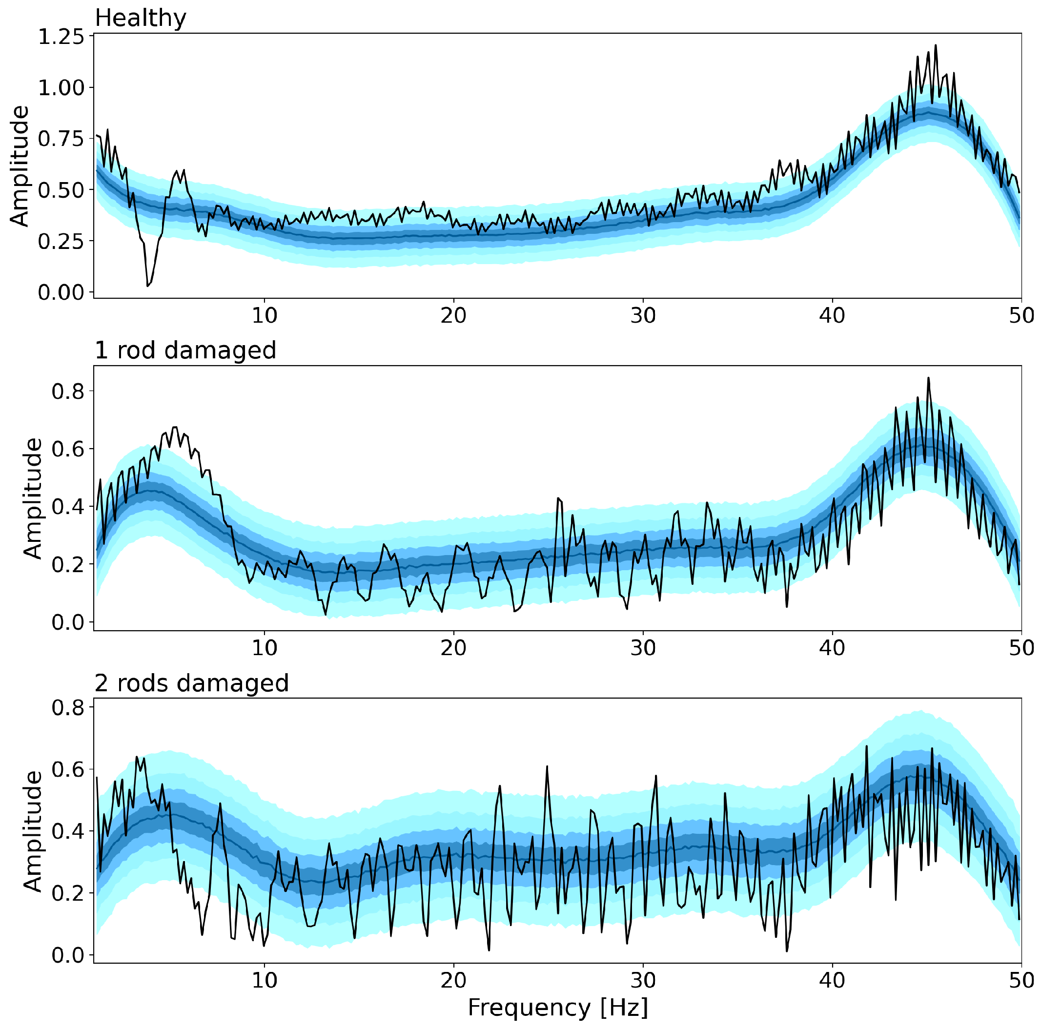
Once the posterior distributions for $(\beta ,\sigma )$ were obtained for each signal class, new spectra could be generated by sampling from the posterior and evaluating the resulting spline expansions. These posterior predictive samples provide plausible spectral curves consistent with the observed data and reflect both natural variability and uncertainty arising from the limited dataset. Examples of such generated curves for the binary classification setting are shown in Figure 9, while Figure 10 displays the corresponding predictive distributions for the three-class case. These results illustrate how the Bayesian functional representation captures the characteristic shape of each class while accommodating the variability inherent in real measurements.

3.2. Gaussian Mixture Modelling of Functional Representations

After obtaining a compact functional representation of each magnitude spectrum, the next step is to formulate a probabilistic classifier capable of distinguishing between the considered motor conditions. Since different classes give rise to characteristic spectral patterns, but the amount of high-quality labelled data is extremely limited, we adopt a mixture-modelling approach built directly on the spline coefficients. Each class is described by a probability density over this coefficient space, allowing both the typical shape and the variability of the spectra to be captured within a unified framework. A mixture formulation then provides a coherent method for assigning class probabilities to new observations using Bayes’ rule.

In our setting, the available information naturally falls into three groups:

• Model-Fitting Data: A small number of labelled examples for each class, together with synthetic spectra generated from the posterior of the spline model. These data anchor the locations and shapes of the class-specific components.
• Regularization Data: Additional unlabelled spectra included during training to stabilize covariance estimates and to prevent the model from overfitting to the idealised variability seen in the synthetic examples.
• Prediction-Time Data: New, previously unseen spectra supplied only for inference, which must not influence the fitted model.

This separation reflects practical constraints common in industrial diagnostics. High-quality labelled recordings require controlled manipulation of equipment and careful verification of fault states, and are therefore scarce. By contrast, unlabelled measurements are abundant but often inconsistent or partially confounded by operating conditions. Incorporating them as regularizing information allows the classifier to learn a realistic variability structure without diluting class definitions. During deployment, the classifier receives only unlabelled operational data and must therefore express uncertainty solely on the basis of what has been learned from the limited training information.

To formalize these ideas, let y denote the vector of spline coefficients obtained from a given spectrum. The distribution of y is modelled as a finite mixture of class-specific Gaussian components:

$$p(y\mid \Theta )=\sum _{m=1}^M{\lambda }_m\mathcal{N}\left(y\mid {\mu }_m,{\Sigma }_m\right),$$

where M is the number of classes, $({\mu }_m,{\Sigma }_m)$ describe the functional variability associated with class m, and ${\lambda }_m$ are the mixture weights. The labelled samples primarily influence the component means, while both labelled and unlabelled samples contribute to estimating the covariance structure, ensuring that the classifier captures realistic uncertainty rather than only the idealised patterns produced by the spline generative model.

The mixture weights $\lambda$ are assigned a Dirichlet prior, which can be tuned to reflect the expected class prevalence or set to be weakly informative when no such information is available. Because the class membership of the unlabelled samples is unknown, these assignments are not treated as discrete latent variables—doing so would introduce discontinuities in the posterior that are incompatible with Hamiltonian Monte Carlo. Instead, their contribution to the likelihood is handled by marginalising over the mixture components, yielding a smooth posterior surface suitable for HMC-based inference.

Figure 11 provides a graphical overview of the model structure. The diagram highlights the roles of labelled and unlabelled data in determining the mixture components and mixture weights, while separating them from the prediction-time data used only for classification. This representation complements the earlier spline model diagram and clarifies how uncertainty propagates from the functional signal representation to the class posterior.

This mixture formulation provides a flexible framework for semi-supervised classification under data scarcity. By combining principled probabilistic modelling of the functional representation with partial information from unlabelled data, the approach yields class probability estimates that reflect both the discriminative structure of the spectra and the inherent uncertainty arising from limited observations.

3.3. Class Probability Reconstruction

Once the mixture model has been fitted, the central task is to determine how likely a new spectrum is to originate from each of the considered motor classes. In a Bayesian framework, this quantity is not obtained from a single, fixed set of parameters, but rather by integrating over all parameter values that are plausible under the posterior distribution. This is a key distinction from classical machine learning classifiers, which evaluate a deterministic model after training. Here, every posterior draw represents one admissible configuration of mixture weights, component means, and covariances, and classification is carried out by averaging the predictions of thousands of such models.

Let y denote the spline coefficient vector of a new spectrum. For a single posterior draw s containing parameters ${\{{\lambda }_m^{\left(s\right)},{\mu }_m^{\left(s\right)},{\Sigma }_m^{\left(s\right)}\}}_{m=1}^M$, Bayes’ rule yields the class membership probability

$$p^{\left(s\right)}(z=m\mid y)={\displaystyle \frac{{\lambda }_m^{\left(s\right)}\mathcal{N}\left(y\mid {\mu }_m^{\left(s\right)},{\Sigma }_m^{\left(s\right)}\right)}{{\sum }_{l=1}^M{\lambda }_l^{\left(s\right)}\mathcal{N}\left(y\mid {\mu }_l^{\left(s\right)},{\Sigma }_l^{\left(s\right)}\right)}}.$$

This quantity describes how a single sampled model instance assigns y to class m.

In practice, the posterior is explored by running four independent Hamiltonian Monte Carlo chains, each producing 1000 post-warm-up draws, yielding approximately 4000 samples. Every one of these samples corresponds to a complete, coherent model that is compatible with the observed data. To obtain the final class probability, we average over all such models:

$$p(z=m\mid y,\mathrm{data})\approx {\displaystyle \frac{1}{S}}\sum _{s=1}^S{p}^{\left(s\right)}(z=m\mid y),S\approx 4000.$$

The associated standard deviation across the S posterior draws provides a natural measure of classification uncertainty.

This procedure embodies the Bayesian principle that inference should reflect not only the most likely model parameters but also the uncertainty associated with them. Instead of committing to a single decision boundary, the classifier aggregates predictions across the entire posterior, producing probability estimates that remain stable even under limited data and that increase in uncertainty when the evidence is ambiguous. Such behaviour stands in contrast to classical discriminative models, where uncertainty is typically a by-product of the link function or calibration procedure, rather than a consequence of integrating across a distribution of plausible models.

The resulting averaged probabilities are used both to assign classes in the test set and to analyse the reliability of each prediction. Signals lying near the overlap of mixture components or associated with limited information naturally exhibit larger posterior variability, which serves as a diagnostic indicator for potential anomalies or borderline cases.

3.4. Computational Fidelity Assessed by Simulation-Based Calibration

Bayesian inference provides not only point estimates but full probability distributions over all unknown parameters. Because our classifier relies directly on these posterior distributions—both for generating synthetic spectra and for averaging predictions over thousands of parameter draws—it is essential to verify that the numerical inference procedure behaves consistently with the underlying statistical model. To this end, we employ simulation-based calibration (SBC), a diagnostic technique that checks whether the posterior inference algorithm recovers known parameter values when data are simulated from the model itself.

The core idea is straightforward: First, parameters are drawn from the prior and used to generate synthetic spectra through the spline-based likelihood. Next, the inference pipeline is executed exactly as in the real analysis, producing posterior samples for each parameter. For a well-calibrated inference algorithm, the true parameter values should appear indistinguishably from random draws taken from the posterior; equivalently, the rank statistics of the true values among the posterior draws should follow a uniform distribution. This provides a direct validation of the computational machinery rather than of the model assumptions themselves.

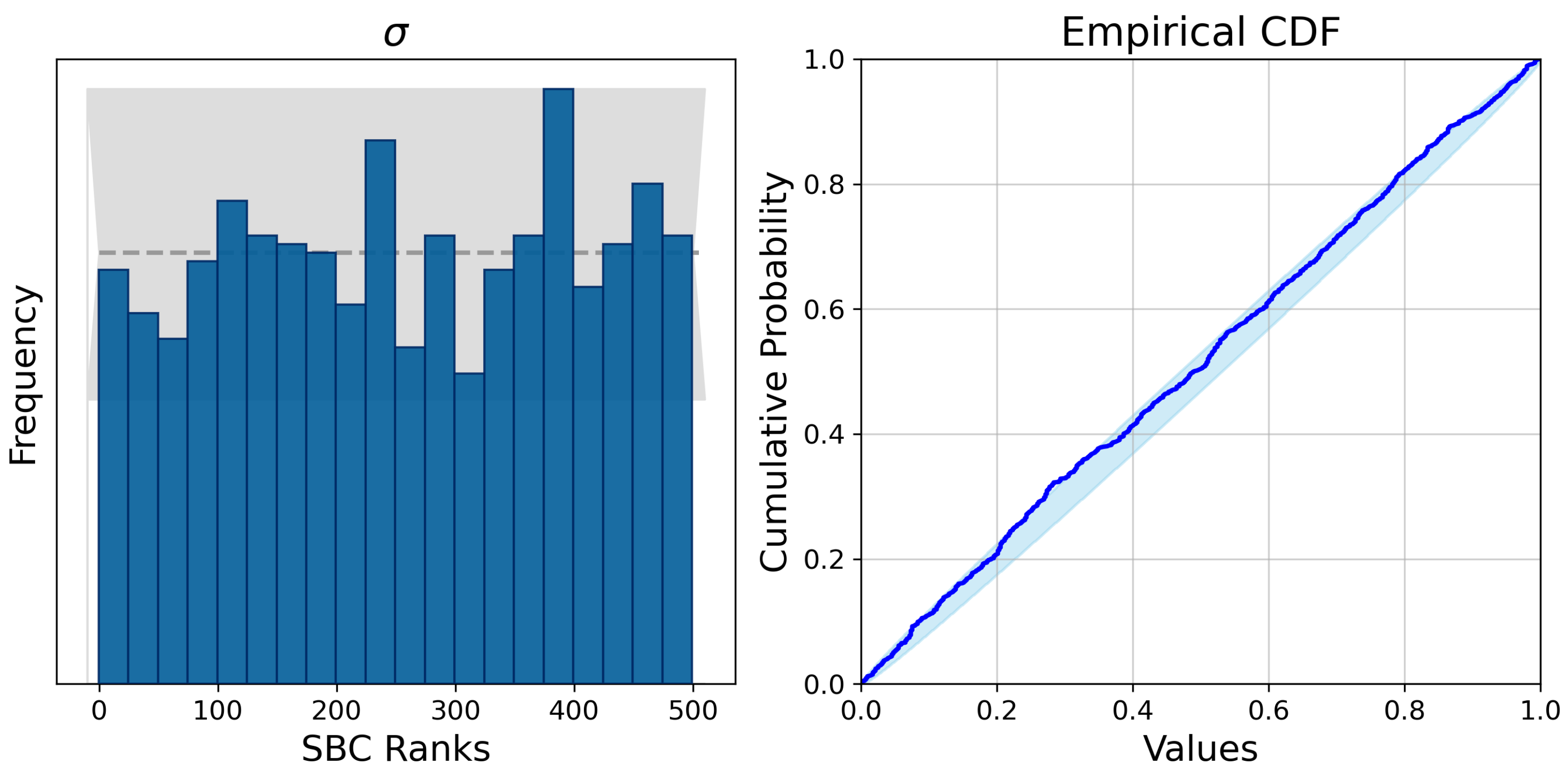
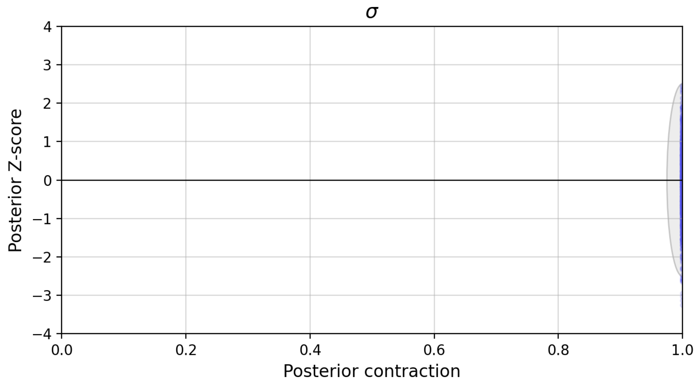
Figure 12 presents rank histograms and empirical cumulative distribution functions (ECDFs) for the noise-scale parameter $\sigma$. The ranks lie well within the theoretical confidence envelope, and the ECDF closely follows the expected diagonal, indicating that the sampler explores the posterior distribution without systematic bias. Complementary information is provided in Figure 13, which displays posterior Z-scores versus posterior contraction. The score cloud lies within the region associated with accurate posterior recovery, demonstrating that the sampler concentrates appropriately around the true parameter values across repeated simulations.

Taken together, these diagnostics show that the Hamiltonian Monte Carlo inference used throughout this paper is numerically reliable. Since classification relies on averaging predictions over approximately 4000 posterior draws, such verification is crucial: any systematic distortion of the posterior would directly affect both the generated training spectra and the class probability estimates. The SBC results therefore provide strong evidence that the Bayesian computations underlying our classifier operate as intended.

4. Results

In this section, we first describe our setup, then give examples of binary and three-class classifiers, and then provide statistical analysis of classifier performance, which are subsequently compared with logistic and soft-max regression. We end the section with a proposed solution for anomaly detection.

4.1. Computation and Learning Setup

The Bayesian classifier operates directly on the spline coefficients obtained from the functional representation of the filtered start-up spectra. Posterior inference for both the spline model and the Gaussian mixture classifier is carried out using the Hamiltonian Monte Carlo with four independent chains and 1000 post-warm-up draws per chain. Each classification result therefore reflects an average over approximately 4000 posterior samples.

The dataset comprises 25 measured spectra: six from a healthy motor, nine from a rotor with a single broken bar, and ten from a rotor with two broken bars. To construct a training dataset that reflects both class structure and within-class variability, we combine real labelled examples with synthetic spectra drawn from the posterior predictive distribution of the spline model. For each class, one real spectrum is selected as a labelled example, and seven posterior predictive samples are generated to complement it. In addition, one real spectrum and twenty-one synthetic spectra drawn from randomly selected classes are included as unlabelled regularization data, following the semi-supervised strategy described earlier.

This procedure is repeated independently across multiple training–testing splits. In each run, labelled examples and unlabelled spectra are resampled according to the above strategy, while the remaining real spectra are set aside for evaluation. This design allows us to assess the robustness of the classifier with respect to the limited availability of high-quality labelled data, and to quantify the stability of its probabilistic predictions under repeated training.

4.2. Binary Classifier Results

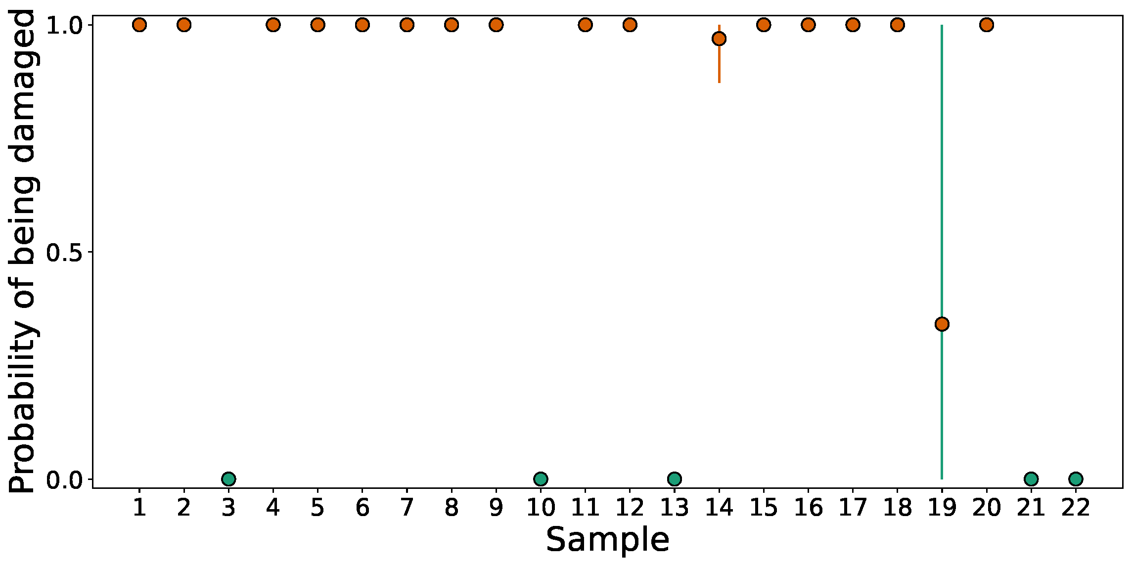
To illustrate the behaviour of the Bayesian mixture classifier in the two-class setting, Figure 14 presents the posterior class probabilities for the held-out spectra across one representative training–testing split. Each point corresponds to the probability assigned to the “damaged” class for a single spectrum, with error bars indicating the posterior standard deviation of the probability estimate across all posterior draws.

The classifier cleanly separates healthy from damaged cases in this example. Spectra originating from healthy motors exhibit probability masses concentrated near zero, and the uncertainty around these estimates is minimal due to the clear spectral differences observed in the low-frequency region. For damaged motors, the model assigns consistently high probabilities to the damaged class, although the magnitude of uncertainty varies across samples. This variation reflects the Bayesian nature of the approach: each probability estimate is obtained by averaging predictions across thousands of posterior parameter configurations, and samples whose spectra resemble the boundary between healthy and damaged behaviour naturally produce wider predictive distributions.

The figure also illustrates a key qualitative feature of the model. A small number of damaged samples yield broader error bars, indicating that their frequency-domain characteristics do not align as cleanly with either class prototype. Such behaviour is expected in semi-supervised mixture models, where uncertainty communicates not only the difficulty of the classification task but also the variability within the modelled classes. Rather than forcing a hard assignment, the classifier expresses this ambiguity through posterior dispersion, which can be valuable when using the results to guide maintenance decisions.

4.3. Three-Class Classifier Results

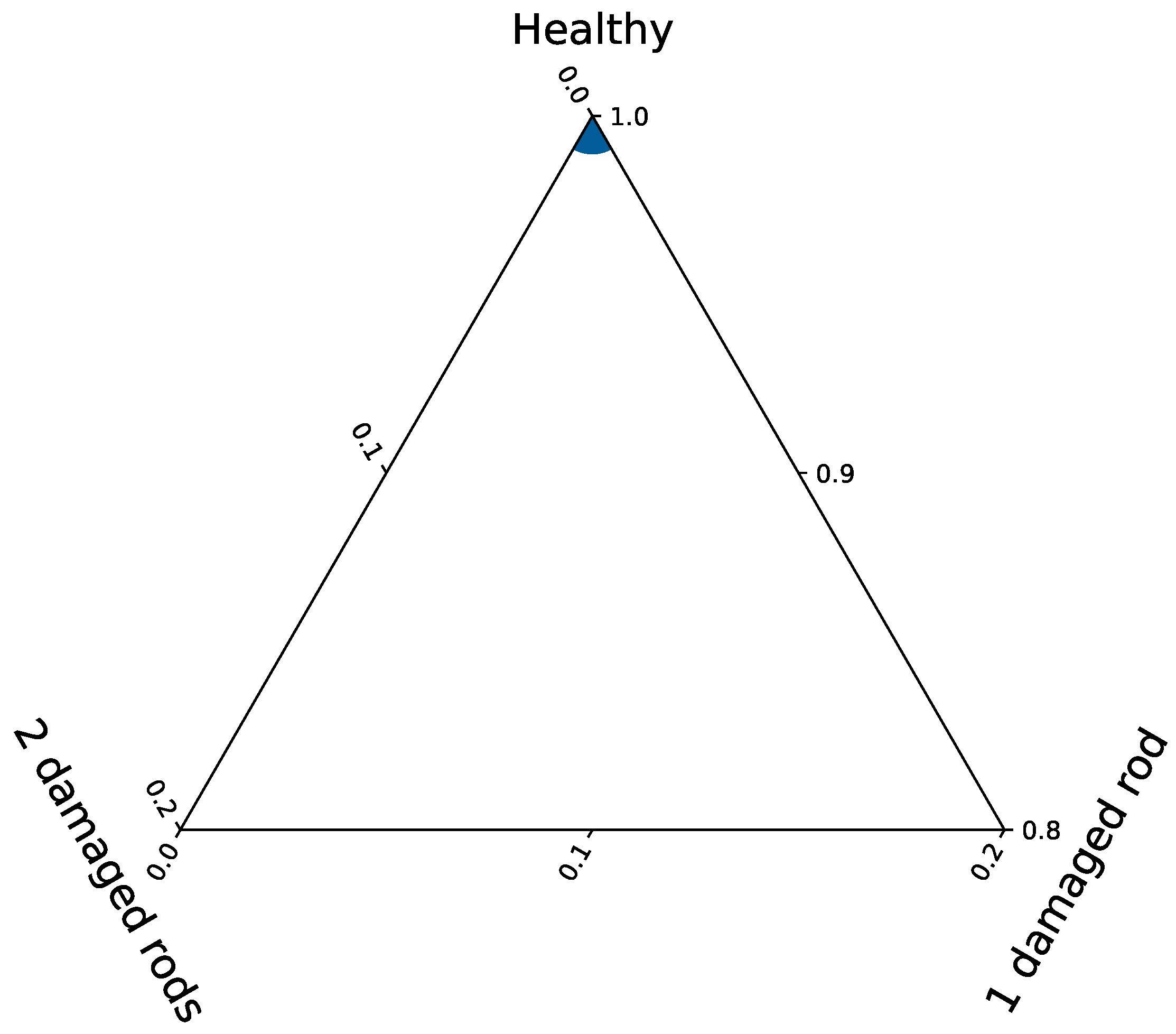
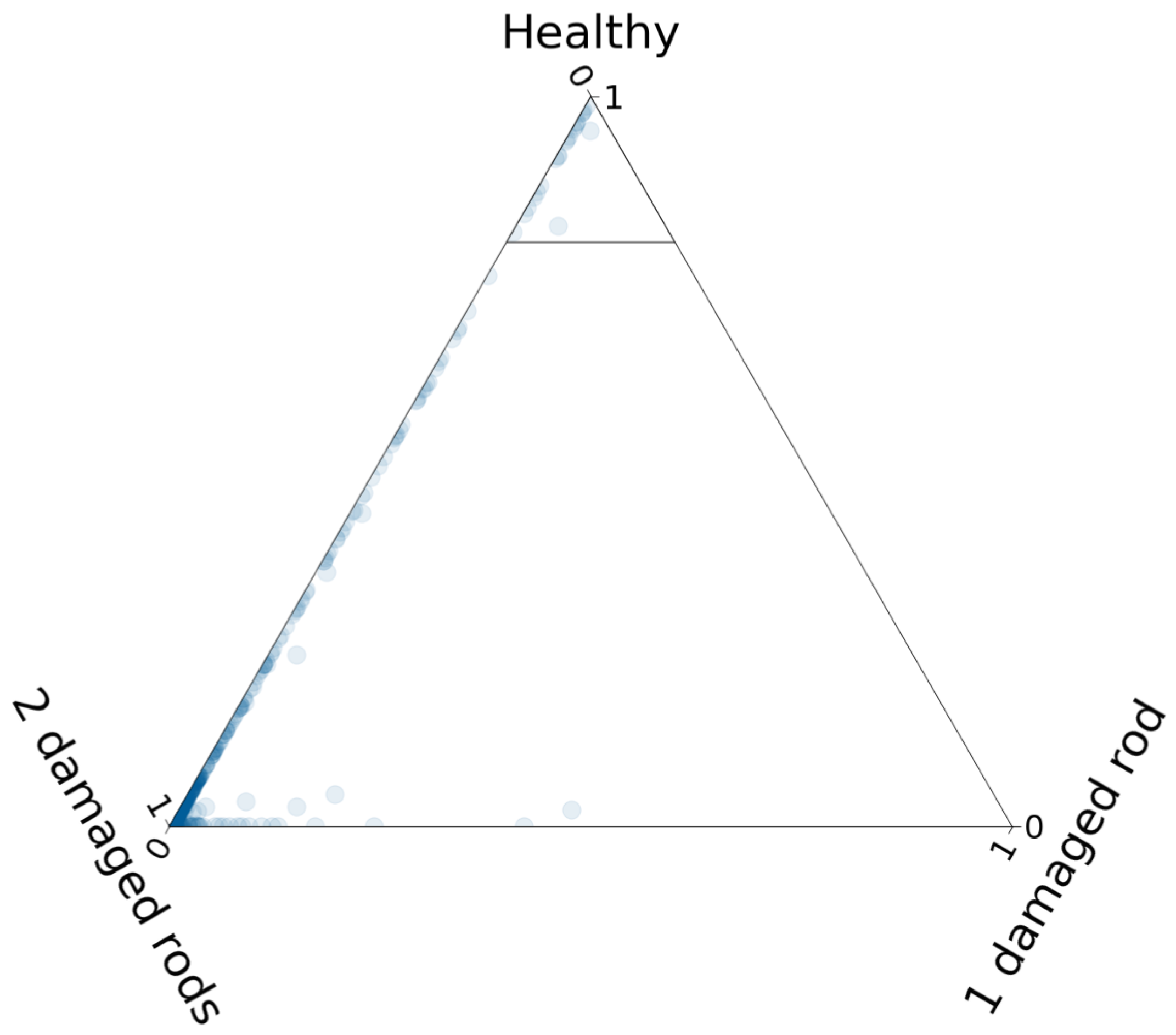
The three-class setting introduces a more demanding discrimination task, as the spectral signatures associated with one and two broken rotor bars are partially overlapping and differ more subtly than those between healthy and damaged motors. Figure 15 illustrates the posterior class probabilities for a representative test split, displayed on a ternary diagram in which each vertex corresponds to one of the three motor conditions.

Healthy spectra form a distinct cluster near the corresponding vertex, reflecting their characteristic low-frequency behaviour and the relative ease with which they can be separated from faulty conditions. In contrast, spectra originating from motors with one or two broken bars occupy broader regions of the simplex. This dispersion is expected: the frequency-domain differences between these two fault types, although present, are less pronounced than those distinguishing healthy from damaged motors. As a result, the mixture model allocates posterior mass across the two faulty classes in proportions that reflect both the evidence in the spectrum and the uncertainty inherent in the learned component distributions.

The spread of probability mass over the simplex provides a compact visual summary of classification confidence. Spectra lying close to a vertex indicate strong posterior support for a single class, whereas points located between vertices reveal ambiguity in class membership. Rather than forcing a hard assignment, the Bayesian classifier expresses such ambiguity through wider posterior distributions, which is particularly useful in fault analysis, where the severity of rotor asymmetry may evolve gradually.

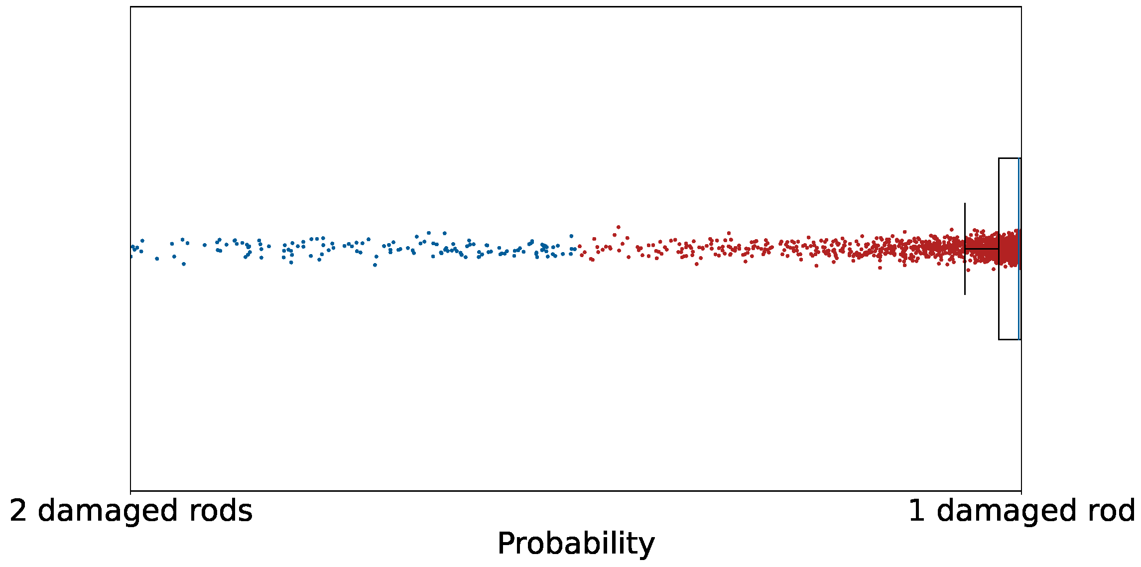
A complementary perspective is provided in Figure 16, which shows the posterior class probabilities for a spectrum whose features place it near the boundary between the two damaged classes. Rather than collapsing onto a single class, the posterior allocates non-negligible probability mass to both fault types, and the variability across posterior draws is substantially larger than in the confident cases. This behaviour reflects genuine ambiguity in the frequency-domain signature of the signal and illustrates how the Bayesian classifier communicates uncertainty when the evidence does not clearly support one fault type over another. Such posterior dispersion is valuable in diagnostic settings, as it highlights spectra that may correspond to transitional damage states or measurement conditions that differ from those represented in the labelled training set.

4.4. Statistical Evaluation Across Repeated Training Runs

To assess the stability of the classifier and its sensitivity to the choice of training samples, we repeated the training–testing procedure one hundred times. In each run, labelled examples and unlabelled spectra were resampled as described earlier, while the remaining real spectra served as the test set. Because classification in the Bayesian framework is performed by averaging predictions over the posterior draws of the mixture-model parameters, each probability estimate reflects the combined effect of model uncertainty and training-data variability. The summary statistics reported below refer to the distribution of posterior mean probabilities across all repeated runs.

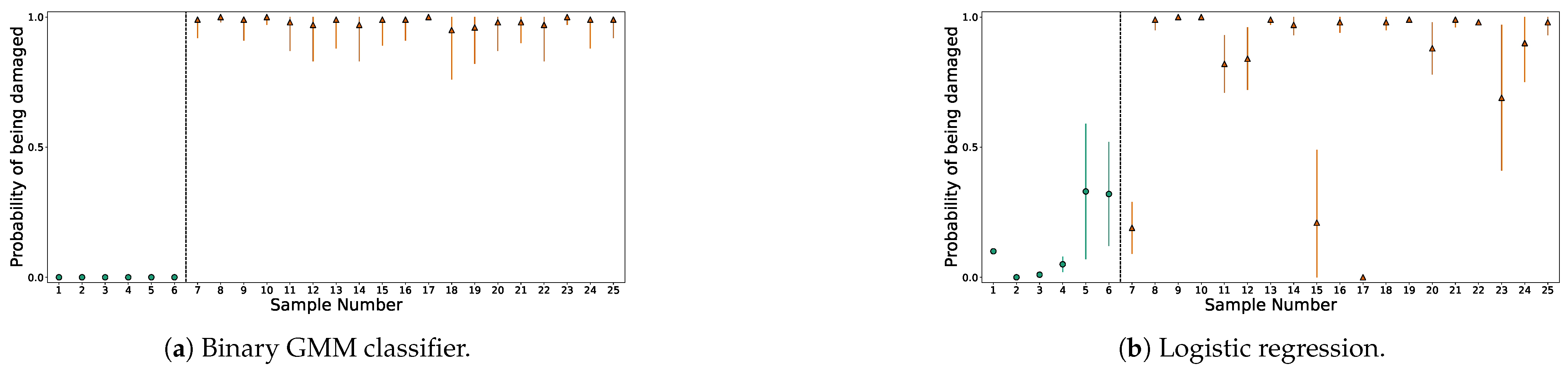
Figure 17a presents the results for the binary classifier. Healthy spectra exhibit posterior probabilities near zero in every run, with negligible spread, indicating that their low-frequency characteristics are consistently separated from those of damaged motors. Damaged spectra show slightly larger variability, as expected for signals that occupy a broader region of the feature space, yet the posterior always places the majority of probability mass on the damaged class. Across all repetitions, the binary classifier assigned more than 50% posterior probability to the correct class for every spectrum, and the dispersion remained modest, reflecting a stable separation between healthy and damaged behaviour.

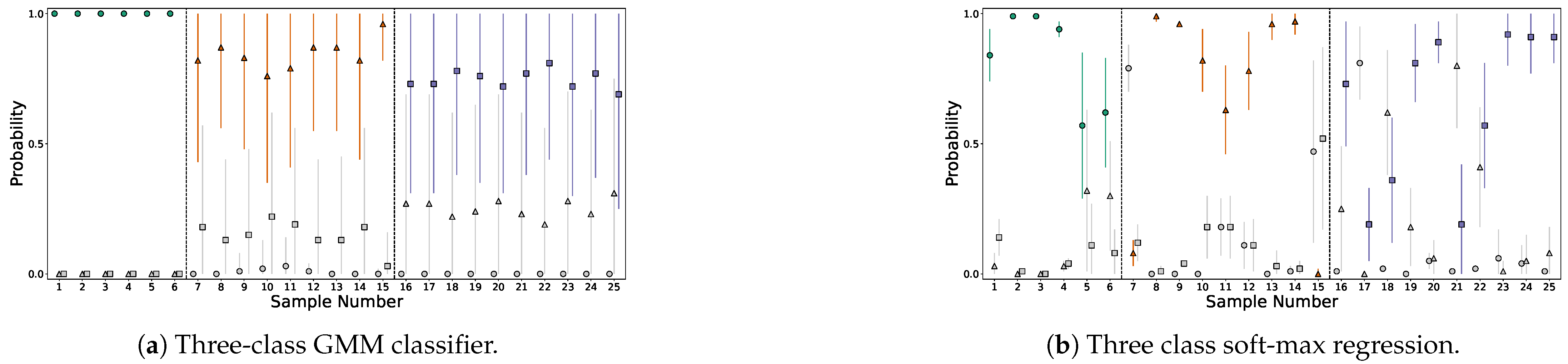
The three-class classifier exhibits a richer structure. Figure 18a summarizes the posterior probabilities for all test spectra over the one hundred runs. Healthy samples again form a compact group with near-zero probability of belonging to either fault class. For the two faulty classes, the posterior mass is typically concentrated on the correct component, but with appreciable run-to-run variability. This is consistent with the partial overlap between the one-bar and two-bar damage signatures and with the semi-supervised nature of the mixture model, which uses both labelled and unlabelled data to shape the class distributions. In quantitative terms, the posterior mean probability exceeded 0.5 for the correct fault class in most repetitions, although the difference between the two damaged classes was sometimes small. The spread in posterior allocations therefore conveys meaningful information about the similarity between the two damage modes and highlights signals whose features lie near the boundary between their respective distributions.

Overall, the repeated-run analysis shows that the Bayesian classifier produces stable and interpretable probability estimates even when training data are scarce. Rather than committing to deterministic labels, the model expresses uncertainty through the posterior distribution of class probabilities, providing a principled way to identify spectra that warrant closer examination or may correspond to intermediate or evolving fault conditions.

4.5. Comparison with Logistic and Soft-Max Regression

To benchmark the Bayesian mixture classifier against more conventional approaches, we implemented a logistic regression model for the binary problem and a soft-max regression model for the three-class case. Both models were trained on the spline coefficients extracted from the frequency-domain representation, using the same resampling scheme as the Bayesian classifier so that the comparison would reflect differences in modelling assumptions rather than training-set composition. The regression models were optimised via standard maximum-likelihood estimation and, thus, produced point estimates of the classifier parameters—in contrast to the Bayesian approach, which aggregates predictions across thousands of posterior draws.

Figure 17 compares the binary classifiers. Logistic regression generally separates healthy from damaged spectra, but the resulting probability estimates show considerable variability across repeated training runs, and several damaged spectra are assigned a probability mass that is inconsistent with their true class. The Bayesian classifier, by contrast, yields posterior probabilities that remain close to the correct class across all repetitions and exhibit narrower spreads. This increased stability is attributable to the mixture model’s ability to integrate information from both labelled and unlabelled data while accounting for parameter uncertainty.

A similar pattern appears in the multiclass comparison (Figure 18). Soft-max regression often identifies the healthy class reliably, but the division between one-bar and two-bar rotor faults is inconsistent, with some spectra alternating between the two classes depending on the particular training split. This behaviour reflects the limited amount of labelled data and the subtle spectral differences between the two fault types. The Bayesian classifier also encounters ambiguity for these cases, but the posterior distribution provides a structured representation of this uncertainty, rather than forcing a single deterministic assignment. As a result, spectra whose features lie near the boundary between the two damage modes are expressed through broader posterior probability intervals rather than abrupt class switching.

Taken together, the comparison indicates that classical regression methods can perform adequately when the classes are well separated, but their predictions become unstable in low-data or overlapping-class regimes. The Bayesian mixture framework offers greater robustness in these settings by explicitly modelling uncertainty in both parameters and data representation, yielding probability estimates that are more coherent across training repetitions and more informative for diagnostic decision-making. Comparisons of logistic and soft-max regressions with GMMs are summarized in the

Table 1. Comparison of GMM and logistic classifiers; probabilities were calculated as statistics over 100 test runs. The sample is considered to be classified if the mean probability of a given sample is equal to or exceeds 0.5, as highlighted with bold numbers. GMM classifiers achieve perfect results, but the confidence of their results is much lower in damaged cases for the 3-class classifier. Logistic classifiers perform much worse in this task, especially in samples with 2 damaged rods.

	GMM Results				Logistic Results
	2-Class	3-Class			2-Class	3-Class
ID	$\mathit{P}\left(\mathit{H}\right)$	$\mathit{P}\left(\mathit{H}\right)$	$\mathit{P}\left(\mathbf{1}\mathit{D}\right)$	$\mathit{P}\left(\mathbf{2}\mathit{D}\right)$	$\mathit{P}\left(\mathit{H}\right)$	$\mathit{P}\left(\mathit{H}\right)$	$\mathit{P}\left(\mathbf{1}\mathit{D}\right)$	$\mathit{P}\left(\mathbf{2}\mathit{D}\right)$
True Label: Healthy
0	1.00 ± 0.00	1.00 ± 0.00	0.00 ± 0.00	0.00 ± 0.00	0.90 ± 0.10	0.84 ± 0.10	0.03 ± 0.05	0.14 ± 0.07
1	1.00 ± 0.00	1.00 ± 0.00	0.00 ± 0.00	0.00 ± 0.00	1.00 ± 0.00	0.99 ± 0.01	0.00 ± 0.00	0.01 ± 0.01
2	1.00 ± 0.00	1.00 ± 0.00	0.00 ± 0.00	0.00 ± 0.00	0.99 ± 0.00	0.99 ± 0.01	0.00 ± 0.01	0.00 ± 0.00
3	1.00 ± 0.00	1.00 ± 0.00	0.00 ± 0.00	0.00 ± 0.00	0.95 ± 0.03	0.94 ± 0.03	0.03 ± 0.02	0.04 ± 0.02
4	1.00 ± 0.00	1.00 ± 0.00	0.00 ± 0.00	0.00 ± 0.00	0.67 ± 0.26	0.57 ± 0.28	0.32 ± 0.31	0.11 ± 0.16
5	1.00 ± 0.00	1.00 ± 0.00	0.00 ± 0.00	0.00 ± 0.00	0.68 ± 0.20	0.62 ± 0.21	0.30 ± 0.21	0.08 ± 0.09
True Label: 1 Damaged Rod
0	0.01 ± 0.07	0.00 ± 0.00	0.82 ± 0.39	0.18 ± 0.39	0.81 ± 0.10	0.79 ± 0.09	0.08 ± 0.05	0.12 ± 0.07
1	0.00 ± 0.02	0.00 ± 0.01	0.87 ± 0.31	0.13 ± 0.31	0.01 ± 0.04	0.00 ± 0.00	0.99 ± 0.02	0.01 ± 0.02
2	0.01 ± 0.08	0.01 ± 0.07	0.83 ± 0.35	0.15 ± 0.33	0.00 ± 0.00	0.00 ± 0.00	0.96 ± 0.04	0.04 ± 0.04
3	0.00 ± 0.03	0.02 ± 0.11	0.76 ± 0.41	0.22 ± 0.40	0.00 ± 0.00	0.00 ± 0.00	0.82 ± 0.12	0.18 ± 0.12
4	0.02 ± 0.11	0.03 ± 0.11	0.79 ± 0.38	0.19 ± 0.37	0.18 ± 0.11	0.18 ± 0.11	0.63 ± 0.17	0.18 ± 0.12
5	0.03 ± 0.14	0.01 ± 0.03	0.87 ± 0.32	0.13 ± 0.31	0.16 ± 0.12	0.11 ± 0.09	0.78 ± 0.15	0.11 ± 0.10
6	0.01 ± 0.11	0.00 ± 0.01	0.87 ± 0.32	0.13 ± 0.32	0.01 ± 0.02	0.00 ± 0.01	0.96 ± 0.06	0.03 ± 0.06
7	0.03 ± 0.14	0.00 ± 0.01	0.82 ± 0.38	0.18 ± 0.38	0.03 ± 0.04	0.01 ± 0.02	0.97 ± 0.05	0.02 ± 0.03
8	0.01 ± 0.10	0.00 ± 0.02	0.96 ± 0.14	0.03 ± 0.13	0.79 ± 0.28	0.47 ± 0.35	0.00 ± 0.02	0.52 ± 0.35
True Label: 2 Damaged Rods
0	0.01 ± 0.08	0.00 ± 0.00	0.27 ± 0.42	0.73 ± 0.42	0.02 ± 0.04	0.01 ± 0.01	0.25 ± 0.24	0.73 ± 0.24
1	0.00 ± 0.01	0.00 ± 0.00	0.27 ± 0.42	0.73 ± 0.42	1.00 ± 0.01	0.81 ± 0.14	0.00 ± 0.00	0.19 ± 0.14
2	0.05 ± 0.19	0.00 ± 0.00	0.22 ± 0.40	0.78 ± 0.40	0.02 ± 0.03	0.02 ± 0.01	0.62 ± 0.24	0.36 ± 0.24
3	0.04 ± 0.14	0.00 ± 0.00	0.24 ± 0.41	0.76 ± 0.41	0.01 ± 0.01	0.00 ± 0.00	0.18 ± 0.15	0.81 ± 0.15
4	0.02 ± 0.11	0.00 ± 0.00	0.28 ± 0.41	0.72 ± 0.41	0.12 ± 0.10	0.05 ± 0.03	0.06 ± 0.07	0.89 ± 0.08
5	0.02 ± 0.08	0.00 ± 0.00	0.23 ± 0.39	0.77 ± 0.39	0.01 ± 0.03	0.01 ± 0.01	0.80 ± 0.24	0.19 ± 0.23
6	0.03 ± 0.14	0.00 ± 0.00	0.19 ± 0.37	0.81 ± 0.37	0.02 ± 0.02	0.02 ± 0.01	0.41 ± 0.23	0.57 ± 0.24
7	0.00 ± 0.03	0.00 ± 0.00	0.28 ± 0.42	0.72 ± 0.42	0.31 ± 0.28	0.06 ± 0.11	0.01 ± 0.04	0.92 ± 0.12
8	0.01 ± 0.11	0.00 ± 0.00	0.23 ± 0.40	0.77 ± 0.40	0.10 ± 0.15	0.04 ± 0.07	0.05 ± 0.10	0.91 ± 0.14
9	0.01 ± 0.07	0.00 ± 0.00	0.31 ± 0.44	0.69 ± 0.44	0.02 ± 0.05	0.01 ± 0.01	0.08 ± 0.10	0.91 ± 0.10

.

4.6. Anomaly Detection

The classifier was also evaluated on data representing a fault type not included among the modelled classes—namely, a rotor with a broken end ring. This scenario was intended to test how the mixture model behaves when confronted with spectra that deviate from the patterns encoded in the labelled training data but still arise from physically plausible motor conditions.

Figure 19 shows the posterior class probabilities for a representative spectrum from this end-ring fault. Unlike the spectra from known classes, which typically generate concentrated posterior mass near a single mixture component, the anomaly produces probability allocations that are markedly diffuse across the three classes. The spread is accompanied by increased variability across posterior draws, reflecting the classifier’s uncertainty regarding how to reconcile the spectral features with the existing class structure.

This response is consistent with the modelling framework. Because the classifier relies on a generative representation of the spectral shapes for the known fault classes, out-of-distribution signals do not force the model toward a confident but erroneous label. Instead, the model distributes posterior mass across components in a way that communicates a lack of support for any single class. In a diagnostic context, such dispersion can serve as an indicator that the observed spectrum does not conform to patterns seen in the training data and, therefore, warrants further examination.

It should be noted that the ability to detect unmodelled faults depends on how distinct their spectral signatures are from those of the included classes. The end-ring fault exhibits features that overlap with the damaged-bar spectra, leading to inconsistent—but still recognizably atypical—posterior allocations across repeated runs. More systematic anomaly detection would require either explicitly modelling additional fault categories or extending the mixture model with mechanisms designed to identify out-of-distribution behaviour, such as hierarchical priors or dedicated uncertainty thresholds.

Overall, the end-ring example demonstrates that the Bayesian classifier can provide informative signals when encountering spectra that fall outside the modelled data manifold, even if it cannot fully characterize such cases within the current class structure.

5. Discussion

The proposed Bayesian mixture model classifier provides a structured way to analyse frequency-domain representations of start-up currents, particularly in situations where only a limited number of labelled measurements are available. By combining functional representations of spectra with probabilistic modelling of class structure, the approach yields classification results that remain stable across repeated training runs and convey meaningful information about uncertainty. This is especially advantageous in motor diagnostics, where measurement conditions vary, class boundaries are not always sharp, and subtle changes in spectral content can signal early stages of rotor degradation.

A key outcome of this study is the distinction between the ease of separating healthy operation from rotor-bar faults and the more nuanced task of distinguishing between different degrees of rotor-bar damage. Healthy spectra possess distinct low-frequency characteristics that allow the classifier to assign posterior mass almost exclusively to the healthy class. Faulty spectra, by contrast, occupy overlapping regions of the feature space—a phenomenon also noted in earlier studies employing transient-current or steady-state analyses [10,11]. The classifier reflects this structure through broader posterior distributions. Rather than indicating a shortcoming of the model, this behaviour captures an important aspect of the underlying physics: the signatures of one and two broken bars are not cleanly separable in all operating conditions, and any diagnosis must contend with this inherent ambiguity.

The results also highlight an important difference between probabilistic mixture modelling and classical regression-based methods. Logistic and soft-max regression can perform adequately when the classes are well separated, but their predictions show greater sensitivity to the specific composition of the training set, particularly when labelled data are scarce. The Bayesian classifier, by directly modelling uncertainty in both spline coefficients and mixture parameters, provides probability estimates that are more coherent across training repetitions and offer a clearer indication of when the data do not strongly support one class over another. In practical terms, this reduces the risk of overconfident or unstable decisions and supports data-driven maintenance strategies that must balance detection sensitivity with operational reliability.

The analysis of the unmodelled end-ring fault further demonstrates the usefulness of uncertainty quantification. Although the classifier does not recognise this fault as belonging to a distinct class, it also avoids forcing a confident assignment to an existing category; instead, the posterior distribution becomes diffuse. This behaviour mirrors observations in other transient analysis studies where atypical or evolving fault conditions produce intermediate spectral features [13]. Posterior dispersion therefore offers a potential route to anomaly detection even without explicit modelling of additional failure modes. However, a systematic treatment of out-of-distribution behaviour would require dedicated extensions to the mixture model or the inclusion of a broader set of fault types in the training process.

Beyond the specific case of rotor-bar faults considered in this study, the proposed framework is not inherently restricted to a particular fault type or machine component. The methodology operates on frequency-domain representations of measured signals and relies on probabilistic modelling of class-specific spectral patterns. As such, it can be extended to other induction motor faults, including stator winding defects or bearing-related asymmetries, provided that the corresponding fault signatures manifest consistently in the analysed signals. The same modelling principles may also be applied to other rotating machinery, such as gearboxes, where vibration, current, or acoustic measurements exhibit characteristic spectral changes under fault conditions. In these cases, the spline-based functional representation and Bayesian mixture classifier would remain unchanged, while the signal type and training data would be adapted to the specific application.

Limitations

Several limitations of the present study should be noted. First, the classifier is trained on a small number of labelled examples, which limits the granularity of the class-specific spline representations and constrains how well within-class variability can be captured. Second, the spectral differences between one and two broken rotor bars are subtle and not universally distinguishable, placing inherent limits on achievable separation regardless of modelling approach. Third, the current mixture model does not implement explicit mechanisms for out-of-distribution detection, and the response to unseen faults—while informative—remains inconsistent across runs. Finally, the spline basis used in this work is manually chosen rather than learned from the data, and alternative bases or adaptive knot-placement strategies could yield improved representation of diagnostically relevant frequency regions.

These considerations motivate several directions for methodological refinement.

Several avenues for future research emerge from these observations. The spline basis used to represent the frequency-domain signals could be adapted to increase resolution in frequency regions that carry diagnostic value, or replaced with sparse or data-driven bases to reduce computational cost. Further improvements in fault discrimination may be achievable through hierarchical mixture structures or through priors that explicitly model progression between different fault states. In addition, incorporating complementary sensing modalities—such as vibration or acoustic emissions—could enhance robustness and support multimodal diagnostic frameworks. Finally, extending the model to identify out-of-distribution signals more systematically would improve its suitability for deployment in real industrial environments, where unexpected or mixed fault conditions are common.

Overall, the results indicate that Bayesian mixture modelling provides a promising foundation for probabilistic condition monitoring of induction motors. Its ability to operate effectively under limited labelled data, quantify uncertainty, and express ambiguity in a principled manner makes it well suited to diagnostic settings in which decisions must be both informative and reliable.

6. Conclusions

This work presents a Bayesian mixture model framework for diagnosing rotor-bar faults in induction motors using frequency-domain representations of start-up currents. By combining functional data analysis with probabilistic classification, the approach provides a coherent means of operating under limited labelled data while offering informative uncertainty estimates for each prediction. The results demonstrate that healthy operation can be distinguished reliably from rotor-bar damage, and that the classifier expresses ambiguity between different damaged states through structured posterior dispersion rather than unstable or overconfident assignments.

A central contribution of this work lies in the integration of Bayesian functional modelling with a probabilistic mixture classifier for start-up current analysis. Unlike conventional transient-based diagnostic methods that rely on deterministic feature extraction or point-estimate classifiers, the proposed approach explicitly models uncertainty at every stage—from spectral representation to class assignment. This enables stable probabilistic predictions under severe data scarcity and provides interpretable confidence measures that are directly relevant for maintenance decision-making.

From an application perspective, the proposed framework is well suited for industrial condition monitoring scenarios where labelled fault data are limited, operating conditions vary, and false alarms carry significant cost. The use of non-intrusive electrical measurements, combined with a probabilistic treatment of uncertainty, makes this approach attractive for deployment as a decision-support tool rather than a rigid fault classifier. Future work may focus on extending the framework to additional fault categories, integrating complementary sensing modalities such as vibration or acoustic emissions, and developing systematic criteria for out-of-distribution detection to support early warning of previously unseen degradation modes.

The comparison with logistic and soft-max regression highlights the benefits of explicitly modelling parameter uncertainty and incorporating unlabelled data during training. Whereas regression-based classifiers exhibit variability across training repetitions—particularly when classes overlap—the Bayesian formulation yields posterior probabilities that remain stable and interpretable even in low-data regimes. The behaviour observed for the unmodelled end-ring fault further suggests that posterior dispersion may serve as a useful indicator of anomalous spectral patterns.

Future developments may include refined functional bases, hierarchical or adaptive mixture structures, and dedicated mechanisms for identifying out-of-distribution signals. The integration of additional sensing modalities also remains a promising direction for improving fault discrimination in complex operating environments. Overall, the findings indicate that Bayesian mixture modelling offers a robust and informative foundation for probabilistic condition monitoring in induction motor applications.