Quantifying Supply-Side Mitigation Strategies for Offshore Wind Energy Droughts on a Global Scale

Abstract

Offshore wind energy offers substantial potential. However, its inherent intermittency leads to the frequent occurrence of offshore wind energy droughts, which pose challenges to electricity system stability. Mitigation measures aim to reduce the number, duration, or impacts of such droughts. Among the different mitigation approaches, supply-side strategies act directly on wind power generation at the wind farm level. Nevertheless, the effectiveness of supply-side mitigation strategies remains poorly understood. This study addresses these gaps by systematically quantifying the potential of three supply-side mitigation strategies: (i) spatial diversification of wind farm locations, (ii) advances in wind turbine technology, and (iii) reductions in downtime and wake losses, to minimize the number and duration of wind energy droughts across 40 key exclusive economic zones (EEZ) worldwide. Hourly, daily, and monthly drought characteristics for both moderate and extreme offshore wind energy droughts are analyzed using wind data from the ERA5 reanalysis for the period 1993–2022. The results show that spatial diversification across multiple sub-regions is the most effective strategy for mitigating offshore wind energy droughts at the EEZ scale. In addition, the effectiveness of all mitigation strategies exhibits pronounced scale-dependent limitations, which are most evident at the monthly time scale. Overall, this study provides a robust basis for energy-policy decisions and highlights the importance of supply-side mitigation for enhancing the reliability of future electricity systems.

1. Introduction

Human activities such as energy production, transportation, agriculture, industry, and deforestation are major contributors to rising greenhouse gas emissions and are ultimately driving global air temperature increases [1]. This anthropogenic climate change has widespread adverse impacts on ecosystems, human health, agriculture, and the availability of essential resources such as water and food [2]. The power sector, in particular, is responsible for approximately 40% of global energy-related CO₂ emissions [3], highlighting the urgency of transitioning to renewable sources of electricity generation for effective climate change mitigation [4]. Among renewables, solar, wind, hydro, biomass and biogas, and geothermal collectively supply the majority of renewable energy production worldwide [5].

The expansion of wind energy is of considerable importance for further increasing renewable power generation and supporting the worldwide decarbonization. Within the realm of wind energy, a distinction is made between onshore and offshore installations based on their location. As of 2024, onshore wind accounts for a significantly larger share of total installed wind capacity, at 93%, compared to offshore wind [6]. However, owing to more abundant wind resources, offshore wind is increasingly recognized as a key pillar of the future power sector.

Like onshore wind, offshore wind is also an intermittent resource, as wind speed (U) over the ocean fluctuates across multiple temporal scales [7]. To capture this variability, wind resource availability is typically analyzed over different periods, such as hours [8], days [9], months [10], and years [11].

At any of these time scales, there may be intervals when the wind resource is minimal or entirely absent [12]. If such low-wind conditions persist over extended periods and affect large geographic areas, they are termed wind energy droughts [13]. Offshore wind energy droughts do not merely represent a loss of energy yield but constitute a systemic risk for power systems with a high reliance on renewable electricity generation.

While numerous studies have examined the number and duration of onshore wind energy droughts at both local and global scales [14,15,16,17,18], research on offshore wind energy droughts remains comparatively scarce. Existing studies are largely limited to regional case studies such as the North Sea [19], the Canary Islands [20], or the Spanish coast [21].

Offshore wind energy droughts are not entirely unavoidable, and their impacts can be mitigated to some degree. Drought mitigation refers to measures aimed at reducing the number, duration, or impacts of periods of anomalously low offshore wind power generation. Such mitigation can be pursued through different approaches, including demand-side strategies that adapt electricity consumption to variable wind power availability [22], system-level measures such as energy storage or grid integration [23], and supply-side strategies that act directly on wind power generation at the wind farm level [24]. While demand- and system-side approaches primarily buffer the consequences of wind energy droughts, supply-side strategies directly influence their number and duration.

Spatial diversification of wind farm sites [25] represents a key supply-side strategy for mitigating wind energy droughts. By distributing offshore wind farms across regions characterized by different wind regimes, the probability that all sites simultaneously experience low U values is reduced [26]. This strategy becomes particularly relevant for large-scale offshore deployment, where aggregated power generation increasingly depends on the spatial coherence of regional wind resource patterns.

Reductions in downtime and wake losses represent operational supply-side strategies that directly affect the power output of offshore wind farms. Wake losses arise from aerodynamic interactions between wind turbines [27], whereas downtimes are primarily related to maintenance and operational constraints [28]. Both factors can substantially reduce power generation [29] and are therefore particularly critical during periods of already limited wind resource availability, as they may accelerate the onset of wind energy droughts. Consequently, optimizing wind farm layouts and maintenance strategies can minimize avoidable losses and reduce the number and duration of wind energy droughts.

Technological advancements in wind turbine design constitute a further important supply-side mitigation pathway [30]. Offshore wind turbines have become significantly more powerful in recent years, with new models commonly rated between 8 and 12 MW [31]. Looking to the future, the IEA 15 MW and NREL 18 MW turbines represent the next generation of technology, while the recently introduced IEA 22 MW turbine signals further advancements in offshore wind capabilities [32]. However, the impact of this development on offshore wind energy droughts is unknown. In particular, it remains unclear whether technological improvements primarily affect average energy yields or also alter the number and duration of offshore wind energy droughts.

Despite the growing importance of offshore wind energy, the scientific literature still exhibits significant limitations and open questions regarding offshore wind energy drought mitigation. In particular, the extent to which wind farm-level interventions, including (i) spatial diversification of wind farm locations, (ii) advances in wind turbine technology, and (iii) reductions in downtime and wake losses, can mitigate wind energy droughts in exclusive economic zones (EEZs), remains insufficiently investigated. This study addresses this gap by providing a comprehensive quantitative assessment of supply-side mitigation strategies for offshore wind energy droughts. The analysis is deliberately confined to supply-side, wind farm-level mitigation measures. Furthermore, this study explicitly distinguishes between wind energy droughts occurring at different temporal scales, given the substantial differences in their characteristics and impacts on power systems, and evaluates mitigation effects for both moderate and extreme offshore wind energy droughts.

2. Materials and Methods

The assessment of supply-side mitigation strategies for moderate and extreme offshore wind energy droughts across hourly, daily, and monthly time scales involves several key steps. First, a dataset of wind farm sites is prepared. Subsequently, the capacity factors (CF) related to wind farms are calculated, utilizing the fifth-generation atmospheric reanalysis of the global climate (ERA5) wind resource data, yielding the “BASELINE” scenario. Then, spatial aggregation and temporal aggregation at hourly, daily, and monthly resolutions of CF are performed, yielding EEZ-wide CF time series. This is followed by calculating moderate and extreme wind energy droughts for 40 EEZs. The wind energy droughts are defined by percentile thresholds of CF. A comprehensive evaluation of the impacts of wind energy drought mitigation strategies was performed with varying factors for wind turbine technology, wake losses, and downtimes. In addition, the effects of spatial diversification of offshore wind farms on wind energy droughts are being investigated by evaluating the wind energy drought properties in 61 marine ecoregions (MEs).

All data processing, analyses, and visualizations were carried out using MATLAB R2025a (The Mathworks Inc., Natick, MA, USA) and ArcGIS Pro 3.6 (Esri Inc., Redlands, CA, USA).

2.1. Wind Farm Site and Resource Data

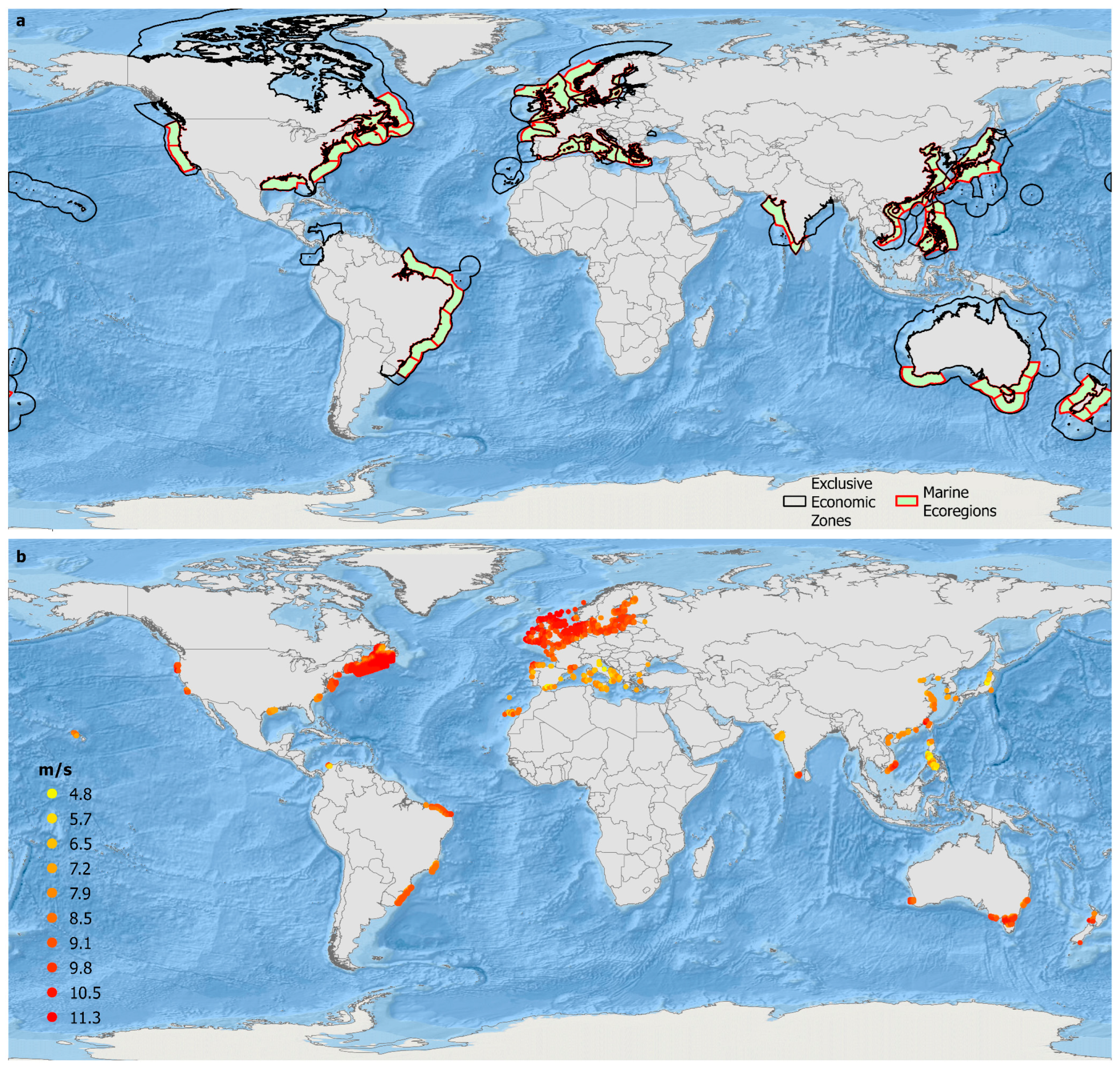
Existing, planned, and potential wind farm sites from 40 EEZs (Figure 1a) were investigated. The wind farm location data were compiled in a previous study [32] from 12 different sources [33,34,35,36,37,38,39,40,41,42,43,44].

Due to the absence of a global measurement network for continuous offshore wind speed at hub height, ERA5 data available 1993–2022 was used [45] to calculate the energy yield of offshore wind turbines. ERA5 generally demonstrated high quality in model validation studies [9,46,47]. However, wind speed estimated by ERA5 may have limitations related to spatial resolution and near-coastal processes. The grid spacing may smooth fine-scale coastal wind speed gradients. In addition, some atmospheric stability effects are only implicitly represented. Thus, previous studies found biases in coastal regions [48] or at high U values [49]. Nevertheless, its consistent global coverage and demonstrated skill make ERA5 suitable for comparative, percentile-based drought analyses.

For this analysis, the meridional (v) and zonal (u) wind vector components in 10 m (v_10m, u_10m) and 100 m (v_100m, u_100m) were used. These components are available at an hourly temporal resolution and a spatial resolution of 0.25° × 0.25°. Based on the wind vector components, hourly wind speed at 10 m (U_10m) and 100 m (U_100m) was calculated by

$$U=\sqrt{u^2+v^2}.$$

(1)

Next, the U_10m and U_100m values were applied to estimate the wind speed in 150 m (U_150m) by the power law [50]:

$$U_{150\mathrm{m}}=U_{10\mathrm{m}}{\left({\displaystyle \frac{150\mathrm{m}}{10\mathrm{m}}}\right)}^{{\displaystyle \frac{ln\left(\frac{U_{100\mathrm{m}}}{U_{10\mathrm{m}}}\right)}{ln\left(\frac{100\mathrm{m}}{10\mathrm{m}}\right)}}}.$$

(2)

This approach depends on a dynamically calculated power-law exponent derived from U_10m and U_100m for each hour and wind farm site. While ERA5 does not explicitly resolve all stability-related processes, this formulation implicitly captures temporal and spatial variability in atmospheric stability through time-varying wind shear.

Figure 1b presents the global distribution of mean U_150m (${\overline{U}}_{150\mathrm{m}}$) in 1993–2022 at the identified offshore wind farm sites. The highest ${\overline{U}}_{150\mathrm{m}}$ values are found in the North Sea in north-western Europe and on the northern coast of the USA and Canada. In these regions, ${\overline{U}}_{150\mathrm{m}}$ values of 10 m/s are frequently exceeded. The ${\overline{U}}_{150\mathrm{m}}$ values are significantly lower in the Mediterranean region in Europe and in some Asian regions. The offshore wind farm sites in Brazilian and Australian EEZs often have ${\overline{U}}_{150\mathrm{m}}$ values of around 8 m/s.

2.2. Capacity Factor Calculation

A generic power curve (PC(U)) for offshore wind turbines is used to calculate EEZ-wide CF based on U. For the BASELINE scenario, the IEA 15 MW wind turbine [51] was selected. It features a hub height of 150 m, a rated power (RP) of 15 MW, and a rotor diameter of 240 m.

Using PC(U), the wind farm related CF (CF_wf) was calculated by the following equation:

$${CF}_{\mathrm{w}\mathrm{f}}={\displaystyle \frac{PC\left(U\right)}{RP}}{EF}_{wakes}{EF}_{downtimes}.$$

(3)

Spatial aggregation of CF is performed prior to drought identification. Thus, for each country, hourly CF values for the EEZs were calculated by averaging all CF_wf values related to wind farms within each EEZ, yielding hourly CF time series. Subsequently, daily and monthly averages of CF were also determined by temporal aggregation. Temporal aggregation refers to the calculation of daily and monthly mean CF by averaging consecutive hourly CF values.

Reductions in CF resulting from wake effects and downtimes are highly variable and depend on a range of site-specific factors. Wake effects are primarily influenced by turbine spacing, park layout, and turbine size, while downtimes are mainly determined by maintenance practices and site accessibility. In accordance with [52,53] and given the lack of detailed information regarding these characteristics for many current and especially future wind farms, a general efficiency factor (EF) of 90% was assumed for wake effects (EF_wakes) and an additional EF of 90% for downtimes (EF_downtimes).

These values are not intended to represent site-specific conditions, but to provide a consistent baseline for a global sensitivity assessment (see Section 2.4). The efficiency factors, therefore, serve as a simplified representation of wake effects and downtimes, which may vary with wind speed and operational conditions. As wind energy droughts are identified using percentile-based capacity factor thresholds, the analysis focuses on relative exceedance behavior, making the results more sensitive to systematic scenario differences than to the exact absolute efficiency values assumed.

2.3. Wind Energy Droughts Calculation

A wind energy drought event is defined as any continuous sequence of time steps (hours, days, or months) during which CF remains below a defined threshold [13,54]. A drought event starts when CF first falls below the threshold and ends immediately when CF exceeds the threshold for a single time step. No minimum event duration is imposed. Consequently, even single-hour, single-day, or single-month shortfalls are classified as individual drought events at the respective temporal resolution. Drought events occurring at the beginning or end of the time series are fully included in the analysis.

A distinction was made between moderate and extreme drought events:

• moderate ED (ED_mod) was defined using the 20th percentile of CF (P20(CF)) as threshold,
• extreme ED (ED_ex) was defined using the fifth percentile of CF (P5(CF)) as a threshold.

Percentile-based thresholds were chosen to allow for a relative, region-independent identification of wind energy droughts across heterogeneous wind regimes.

The threshold value P20(CF) was selected based on its use in previous research [54,55], as it effectively captures moderate wind energy droughts. Values below this percentile indicate more extreme, and thus rarer, wind energy drought occurrences. In meteorological studies, the 5th percentile is commonly employed to delineate extreme events [56]. Accordingly, this study designates P5(CF) as the threshold for defining extreme wind energy droughts.

Each value of the CF time series is evaluated to see if P20(CF) or P5(CF) is exceeded by [13,15]

$${ED}_{\mathrm{m}\mathrm{o}\mathrm{d}}(t)=\left\{\begin{array}{c}0,CF\left(t\right)\ge P20\left(CF\right)\\ 1,CF\left(t\right)<P20\left(CF\right)\end{array}\right.$$

(4)

and

$${ED}_{\mathrm{e}\mathrm{x}}(t)=\left\{\begin{array}{c}0,CF\left(t\right)\ge P5\left(CF\right)\\ 1,CF\left(t\right)<P5\left(CF\right)\end{array}\right.,$$

(5)

with t the time unit hour, month, or day.

The end of a wind energy drought is marked by ED(t) in the time series, attaining a value of 0. The duration of ED (T) was then calculated. In addition, the average number of hours, days or months per year classified as wind energy droughts (N), as well as the mean number of wind energy drought events per year (NED), was determined. Under the BASELINE scenario, the N values are predefined and identical across all EEZs, as wind energy droughts are based on percentiles. In contrast, the T and NED values may vary across EEZs under the BASELINE scenario.

2.4. Impact of Mitigation Measures

Five scenarios were compared to the BASELINE scenario. These scenarios collectively represent key supply-side strategies to influence offshore wind energy droughts directly at the offshore wind farm level.

Table 1. Evaluated scenarios including wind turbine type, hub height, efficiency factors (EF) for wake effects and downtimes, spatial scale (exclusive economic zone (EEZ), and marine ecoregion (ME)).

Scenario	Turbine	Hub Height	Wake Effects EF	Downtimes EF	Scale	Description of Scenario
BASELINE	IEA 15 MW	150 m	90%	90%	EEZ	baseline
LESS	IEA 15 MW	150 m	95%	95%	EEZ	less wake effects and downtimes
MORE	IEA 15 MW	150 m	85%	85%	EEZ	more wake effects and downtimes
OLD	NREL 5 MW	90 m	90%	90%	EEZ	old wind turbine technology
NEW	IEA 22 MW	170 m	90%	90%	EEZ	new wind turbine technology
REGIONAL	IEA 15 MW	150 m	90%	90%	ME	siting at the marine ecoregion level

summarizes the properties modified in each scenario. The “OLD” scenario assumes the use of the NREL 5 MW wind turbine [51], which was among the dominant types in the global wind turbine fleet until a few years ago [31]. The “NEW” scenario considers the IEA 22 MW turbine [57] as the future dominant type.

The “LESS” and “MORE” scenarios represent either decreases or increases in the reduction for wake effects and downtimes. They constitute a sensitivity analysis of wake and downtime efficiency factors, allowing the robustness of drought frequency and duration metrics to be assessed with respect to variations in these parameters.

Grid-related curtailment also affects CF, but it is not considered in these scenarios, as curtailment typically occurs during periods of wind energy surpluses rather than deficits. Since wind energy droughts are defined by low power output periods, grid curtailment is irrelevant to this analysis.

A “REGIONAL” scenario was developed to quantify the influence of spatial diversification of wind turbines on wind energy droughts. This scenario uses the same fundamental parameters as the BASELINE scenario, but assessments are conducted at the level of MEs [58] within EEZs. Marine ecoregions are areas defined by similar environmental conditions. They were selected as a subnational aggregation unit as they reflect coherent large-scale atmospheric and oceanographic conditions that are relevant for offshore wind variability. The “REGIONAL” scenario is only applied when an EEZ contains multiple MEs.

The methods used to calculate CF as well as T, NED, and N for these scenarios are consistent with those described for the BASELINE scenario. However, a key difference is that the P20(CF) and P5(CF) thresholds are not recalculated for each scenario but instead are adopted directly from the BASELINE scenario. This enables the comparison of the differences in wind energy drought characteristics of all scenarios to the BASELINE scenario.

3. Results and Discussion

The Results and Discussion section contains four subsections. After characterizing CF variability, wind energy droughts under the BASELINE scenario are examined to establish a reference for regional differences and temporal scales. The subsequent subsections show and discuss how wake effects and downtimes, turbine technology, and spatial diversification act as supply-side mitigation measures and alter the number and duration of moderate as well as extreme wind energy droughts.

The results are illustrated comprehensively for six representative countries (China, the UK, Germany, Brazil, the United States, and India) selected due to their high existing offshore wind capacity or substantial future development potential.

Comprehensive data on offshore mitigation statistics for all 40 analyzed EEZs are provided in the Supplementary Materials.

3.1. Capacity Factor Frequency Distributions

Capacity factor frequency distributions provide the statistical foundation for the subsequent analysis of offshore wind energy droughts. They characterize the shape, spread, and asymmetry of wind power variability across regions and temporal scales, which directly determine the percentile-based thresholds used to identify moderate and extreme drought events. All subsequent assessments of wind energy drought occurrence and mitigation effects, therefore, build on changes in these underlying capacity factor distributions.

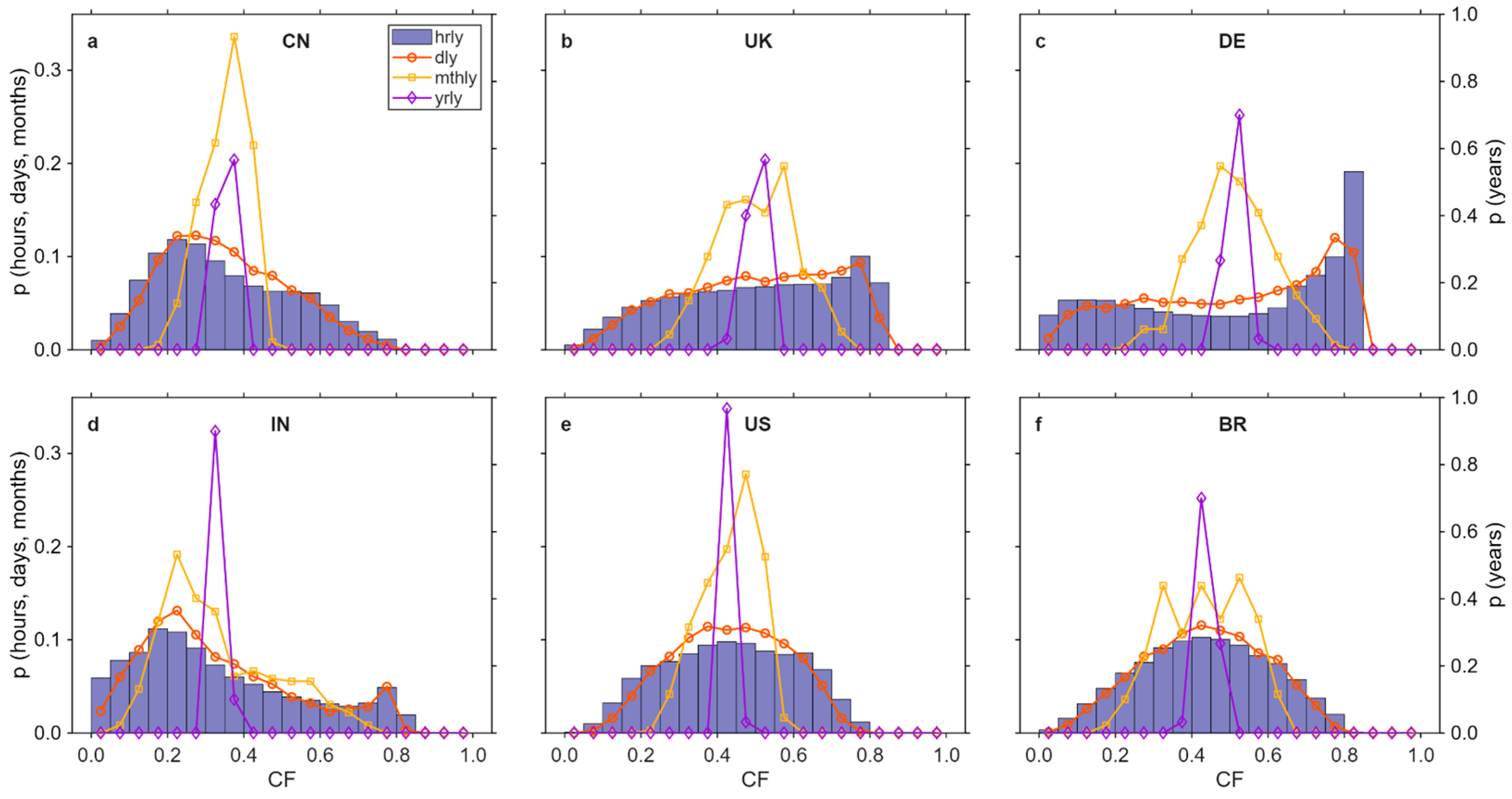
Figure 2 depicts the relative frequency (p) of CF class values across hourly (hrly), daily (dly), monthly (mthly), and yearly (yrly) time scales for EEZs of six chosen countries.

There are substantial differences in the CF distribution not only among EEZs but also across the various time scales analyzed. Generally, the dispersion of CF values increases as the duration of the time scale decreases.

The hourly and daily CF values of China’s EEZ (Figure 2a) are right-skewed, peaking around 0.25. In contrast, the distributions of the monthly and yearly CF values are highly peaked. The most frequent CF class values for monthly and annual CF are around 0.35.

Unlike China, the UK’s hourly and daily CF values exhibit a left-skewed distribution (Figure 2b). The monthly CF values fluctuate considerably, ranging from 0.30 to 0.70, indicating pronounced intra-annual variability. Conversely, the narrow range of annual CF values suggests that inter-annual variability is much less significant.

In Germany’s EEZ, the hourly CF distributions are dominated by the class of 0.81 (Figure 2c). This indicates frequently occurring optimal availability of wind resources, which is subject to limitations caused by wake effects and reduced operational availability. There is also a secondary peak in the hourly CF values below 0.20, while values in the mid-to-high CF range, around 0.50, are rare. Notably, the monthly and annual CF values peak in the range where hourly CF values reach their minimum. This illustrates that the distribution of CF values can vary significantly depending on the temporal resolution.

In the Indian EEZ, the hourly and daily CF distributions are right-skewed (Figure 2d). Unlike the other EEZs, the monthly CF values also display substantial variability and are right-skewed. This underscores the significant intra-annual variability driven by the monsoon [59]. In contrast, the inter-annual variability is low, as shown by the distinctly pronounced peak in the annual CF distribution.

The CF distributions for the US American EEZ are almost symmetric (Figure 2e), indicating that neither extremely low nor extremely high CF values occur at any temporal scale. One possible reason for this is the broad geographic distribution of offshore wind farms within this EEZ.

Similarly, the hourly and daily CF distributions in the Brazilian EEZ are nearly symmetric, like those in the US-American EEZ, with a peak near 0.41 (Figure 2f). The high variability observed in the monthly CF values is pronounced and indicates strong seasonality in the wind resource.

The substantial variability in CF distributions between countries and across the different time scales analyzed is also observed in the other 34 EEZs included in this study. The Supplementary Materials provide a summary of the mean, median, and mode of CF for all EEZs across all time scales. In some small EEZs with limited wind resource, the modal CF value at the hourly and daily scale is 0.00.

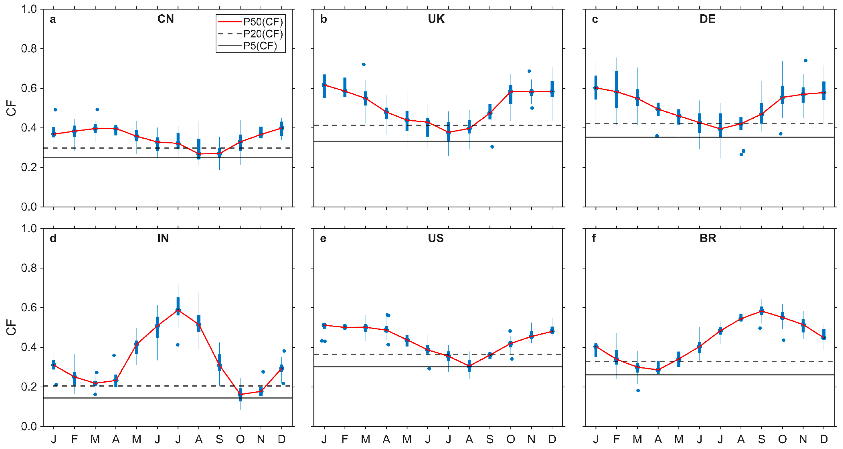
The period of frequent high and low CF values plays a critical role in the predictability and stability of the power supply. Thus, Figure 3 illustrates the annual cycle of monthly CF for 1993–2022. Each of the six EEZs exhibits a distinct seasonal pattern in monthly CF values, though some similarities are apparent among certain EEZs. The mid-latitude EEZs of the Northern Hemisphere, including China (Figure 3a), the UK (Figure 3b), Germany (Figure 3c), and the USA (Figure 3e), consistently have their lowest monthly CF values during the summer months (June, July, August). Their exact timing of the minimum varies by country. India (Figure 3d) records the highest monthly CF values in the summer, while in Brazil (Figure 3f), the peak values occur in September. Another distinguishing feature is the range of monthly CF values. India experiences the most dramatic difference between summer CF values and those during the rest of the year.

The thresholds for moderate and extreme wind energy droughts indicate that monthly wind energy droughts occur more frequently, or even exclusively, during certain months in many countries. For example, in India, no wind energy droughts are observed from May to August, while in Brazil, the wind energy drought-free period lasts from July to December. In contrast, moderate wind energy droughts in Germany are possible almost throughout the entire year.

In addition to seasonal variability, diurnal fluctuations in CF are also a key feature of offshore wind energy generation, affecting hourly wind energy droughts.

3.2. Wind Energy Droughts Under Baseline Scenario

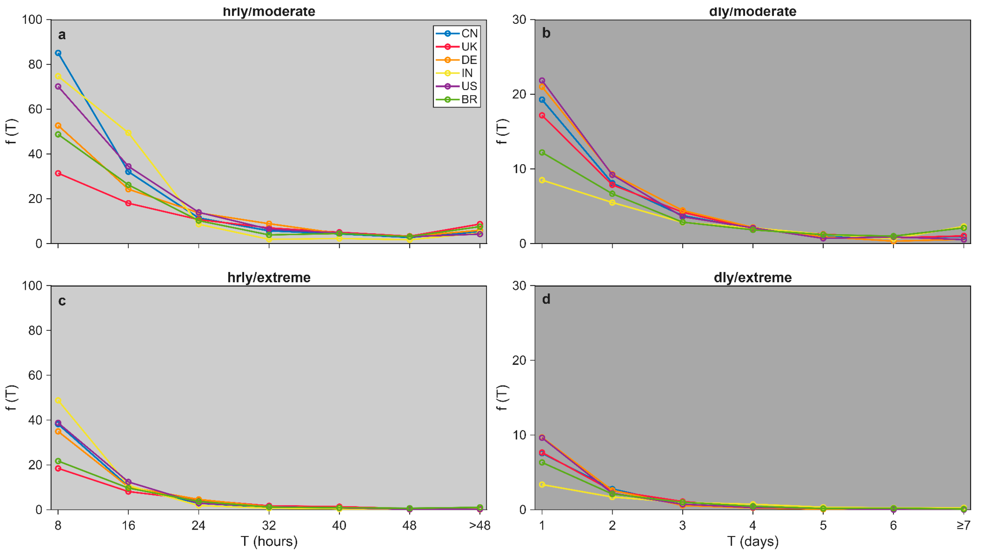
The duration of wind energy drought periods is a key criterion for evaluating their severity. Figure 4 illustrates the (f(T)) for various wind energy drought durations for the BASELINE scenario. A comparison across EEZs reveals both regional differences and overarching patterns. Short-duration wind energy droughts are the most frequent in all regions and across all cases. Specifically, very short droughts (1 day at daily resolution, ≤8 h at hourly resolution) are the most common.

All studied EEZs also experience very long wind energy droughts (>48 h at hourly resolution, ≥7 days at daily resolution). The average number of moderate wind energy droughts per year lasting more than 48 h at hourly resolution ranges from 4.2 in the US to 8.7 in the UK (Figure 4a). The highest value of f(T) for very long and extreme wind energy droughts is observed in Brazil, at 1.0 per year (Figure 4c). Conversely, Germany and Brazil exhibit the lowest frequencies for very long wind energy droughts, with f(T) values of 0.2 per year.

By definition, a wind energy drought at the hourly level ends as soon as CF exceeds the threshold for just one hour. Consequently, a new drought event may begin shortly thereafter if the threshold is again not met. In contrast, analysis at the daily time scale averages out such short-term fluctuations, rendering brief interruptions insignificant for the identification of wind energy droughts. Depending on the specific research objective, this smoothing effect can be either beneficial or limiting.

Consequently, wind energy droughts defined on a daily scale generally have longer durations. Most very long moderate wind energy droughts (lasting 7 days or more) occur in India (2.3 events per year) and Brazil (2.1 events per year) (Figure 4b). In the USA, the frequency is lower, with f(T) = 0.5. Extreme long-duration wind energy droughts are very rare (Figure 4d), occurring most frequently in India, where f(T) reaches 0.3 per year.

Table 2. Mean duration of moderate and extreme wind energy droughts ($\overline{T}$) in the analyzed exclusive economic zones (EEZs) at hourly (hrly), daily (dly), and monthly (mthly) resolution in 1993–2022.

	Hourly		Daily		Monthly
EEZ	Moderate	Extreme	Moderate	Extreme	Moderate	Extreme
Australia	15.0	9.3	1.8	1.4	1.5	1.2
Belgium	10.9	4.8	1.8	1.3	1.5	1.1
Brazil	16.8	11.3	2.6	1.8	2.2	1.6
Canada	17.1	10.0	1.7	1.3	1.9	1.1
Canary Islands	17.2	8.0	2.5	1.6	1.4	1.1
China	12.0	8.1	2.0	1.6	1.8	1.3
Colombia	10.4	2.3	2.7	1.3	1.9	1.2
Croatia	7.0	1.3	1.8	1.4	1.7	1.1
Denmark	17.6	10.0	1.9	1.4	1.6	1.2
Estonia	13.0	6.7	1.9	1.4	1.7	1.1
Finland	14.4	8.2	1.9	1.4	1.6	1.2
France	13.9	7.5	2.1	1.4	1.4	1.2
Germany	15.5	8.4	1.9	1.4	1.8	1.1
Greece	13.2	7.9	1.9	1.4	1.4	1.1
Hawaii	17.5	6.7	2.5	1.4	1.5	1.0
India	12.2	6.9	3.2	2.4	1.5	1.2
Ireland	17.4	9.5	2.0	1.4	1.7	1.1
Italy	15.8	8.7	2.1	1.5	1.6	1.1
Japan	10.7	5.7	2.1	1.5	1.8	1.1
Jersey	10.1	2.3	1.8	1.3	1.6	1.3
Latvia	12.7	6.3	1.8	1.3	1.6	1.1
Lithuania	10.8	5.1	1.8	1.3	1.5	1.2
Madeira	12.2	1.8	2.1	1.4	1.3	1.0
Malta	10.8	1.7	2.2	1.5	2.0	1.1
Netherlands	14.4	7.2	1.8	1.4	1.7	1.1
New Zealand	14.0	7.7	1.9	1.4	1.4	1.1
Norway	15.2	9.0	1.9	1.4	1.8	1.1
Philippines	19.8	7.4	3.7	1.9	1.8	1.3
Poland	12.9	6.1	1.8	1.3	1.4	1.1
Portugal	9.4	4.3	2.0	1.4	1.3	1.3
Romania	7.9	1.6	1.8	1.3	1.6	1.1
Saint Pierre	11.9	5.8	1.6	1.4	1.8	1.1
Republic of Korea	6.8	1.3	1.7	1.2	1.4	1.1
Spain	14.8	8.5	1.9	1.4	1.7	1.1
Sweden	15.4	8.9	2.0	1.5	1.6	1.1
Taiwan	10.0	1.6	2.3	1.3	1.5	1.0
UK	20.8	12.4	2.1	1.5	1.7	1.4
Uruguay	9.0	2.3	1.6	1.2	1.5	1.2
USA	12.8	7.7	1.9	1.4	2.0	1.1
Vietnam	20.3	10.7	3.5	2.0	1.4	1.0

presents the mean T ($\overline{T}$) of wind energy droughts for each combination of temporal resolution and drought intensity across all EEZs. Because the same CF percentiles were applied as thresholds in all EEZs, a relatively short average drought duration corresponds to a relatively high frequency of drought events. For hourly wind energy droughts, the Republic of Korea exhibits the shortest average durations for both moderate ($\overline{T}$ = 6.8 h) and extreme events ($\overline{T}$ = 1.3 h), while the UK experiences the longest durations, with $\overline{T}$ = 20.8 h for moderate and $\overline{T}$ = 12.8 h for extreme droughts. Accordingly, the Republic of Korea has the highest frequency of wind energy droughts, while the UK has the lowest.

At longer temporal resolutions, the spatial pattern shifts: the lowest $\overline{T}$ values for daily wind energy droughts are found in Uruguay, while the highest are observed in the EEZ of the Philippines for moderate droughts ($\overline{T}$ = 3.7 days) and in India for extreme droughts ($\overline{T}$ = 2.4 days).

Due to pronounced monthly variability in CF, Brazil exhibits the highest $\overline{T}$ values at a monthly resolution. The substantial regional differences in $\overline{T}$ highlight the need for strategies that are tailored to local wind energy drought conditions.

3.3. Impact of Wake Effects, Downtimes, and Turbine Technology on Wind Energy Droughts

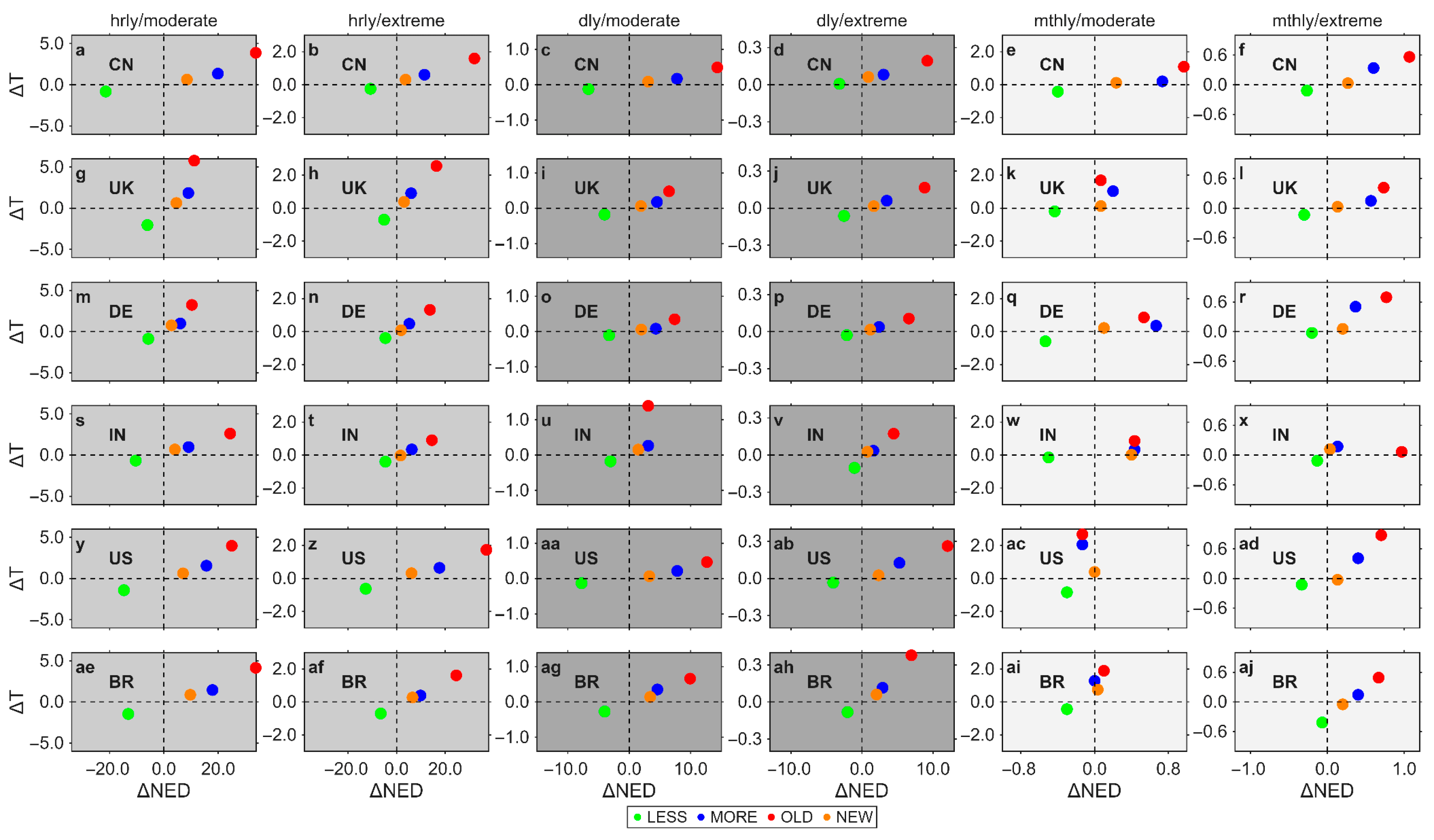
Figure 5 presents Δ$\overline{T}$ and ΔNED for the LESS, MORE, OLD, and NEW scenarios relative to the BASELINE Scenario. Each sub-figure represents a specific combination of temporal resolution, drought intensity, and EEZ under investigation. Within each sub-figure, four quadrants display the changes in NED and $\overline{T}$ with respect to the BASELINE scenario. Moving clockwise, the quadrants correspond to (i) an increase in NED and an increase in $\overline{T}$, (ii) an increase in NED and a decrease in $\overline{T}$, (iii) decrease in NED and decrease in $\overline{T}$ and (iv) decrease in NED and increase in $\overline{T}$. This layout offers a concise visual summary of how changes in wind turbine type and wake effects influence wind energy droughts.

Changes in wind turbine technology, wake effects, and availability have a similar impact on all EEZs. The intensity and time scale of the drought also have no influence on the trend development of NED and $\overline{T}$. However, there are differences in the magnitude of the changes.

The largest impact on both NED and $\overline{T}$ is observed under the OLD scenario, which results in a substantial increase in these metrics. For example, in Brazil, moderate wind energy droughts at the hourly temporal scale exhibit increases of 33.8 per year in NED and 4.1 h in $\overline{T}$ under the OLD scenario. In Germany, the increases are lower, with NED rising by 10.3 per year and $\overline{T}$ by 3.2 h. Current wind turbine fleets more closely resemble the OLD scenario than the BASELINE scenario. Consequently, further development of wind turbine fleets is expected to reduce both NED and $\overline{T}$ associated with wind energy droughts and consequently is an effective mitigation approach.

The differences in wind energy drought characteristics between the OLD, BASELINE, and NEW scenarios reflect the combined effect of increased hub height and modified wind turbine design parameters. The observed mitigation is therefore not driven by hub height alone. In particular, the unfavorable power curve properties of the OLD turbine under low-to-moderate wind speed, associated with its high specific power (401 W/m²), amplify both drought duration and frequency.

The relationship between wind energy drought characteristics and rated power is non-linear, as evidenced by the results of the NEW scenario. Although the NEW turbine features a higher hub height and rated power, both $\mathsf{\Delta }\overline{T}$ and ΔNED remain slightly positive relative to the BASELINE scenario. This can be attributed to two factors: (i) the diminishing increase in wind speed with height at very high hub heights compared to medium hub heights, and (ii) the higher specific power of the NEW turbine (347 W/m²) compared to the BASELINE turbine (332 W/m²), which leads to less favorable power-curve characteristics under low-to-moderate wind speed. Similar behavior has been reported in a previous study [32].

As expected, increased loss due to wake effects and reduced wind turbine availability lead to higher values of both NED and $\overline{T}$. The magnitude of these changes is smaller under the MORE scenario compared to the OLD scenario. For example, in Brazil, moderate wind energy droughts at the hourly temporal scale increase by only 17.9 per year in NED and 1.4 h in $\overline{T}$ under the MORE scenario.

Conversely, the LESS scenario leads to lower NED and $\overline{T}$ values. For the Brazilian example of moderate wind energy droughts on an hourly time scale, ΔNED = −13.1 per year and Δ$\overline{T}$ = −1.5 per year.

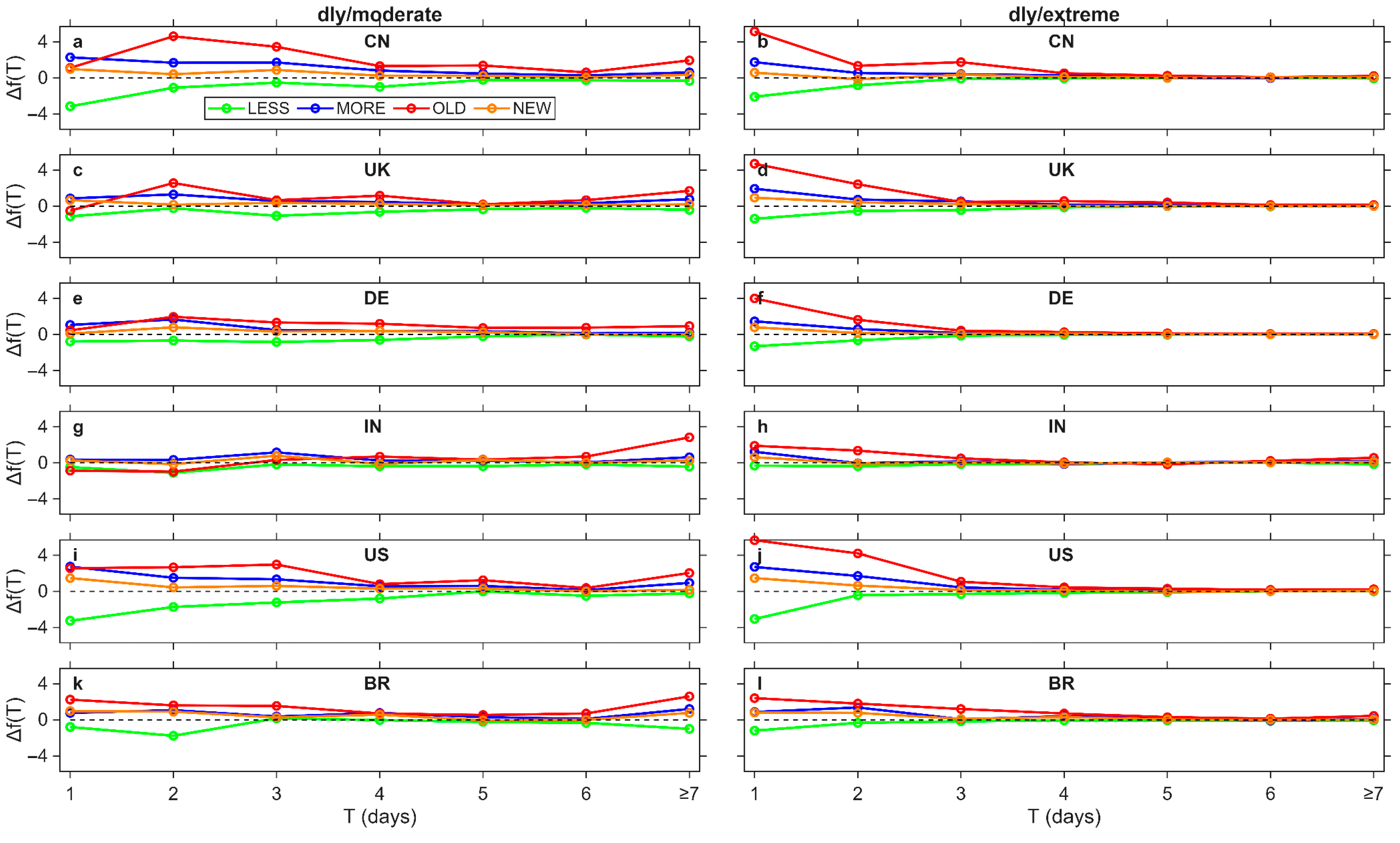
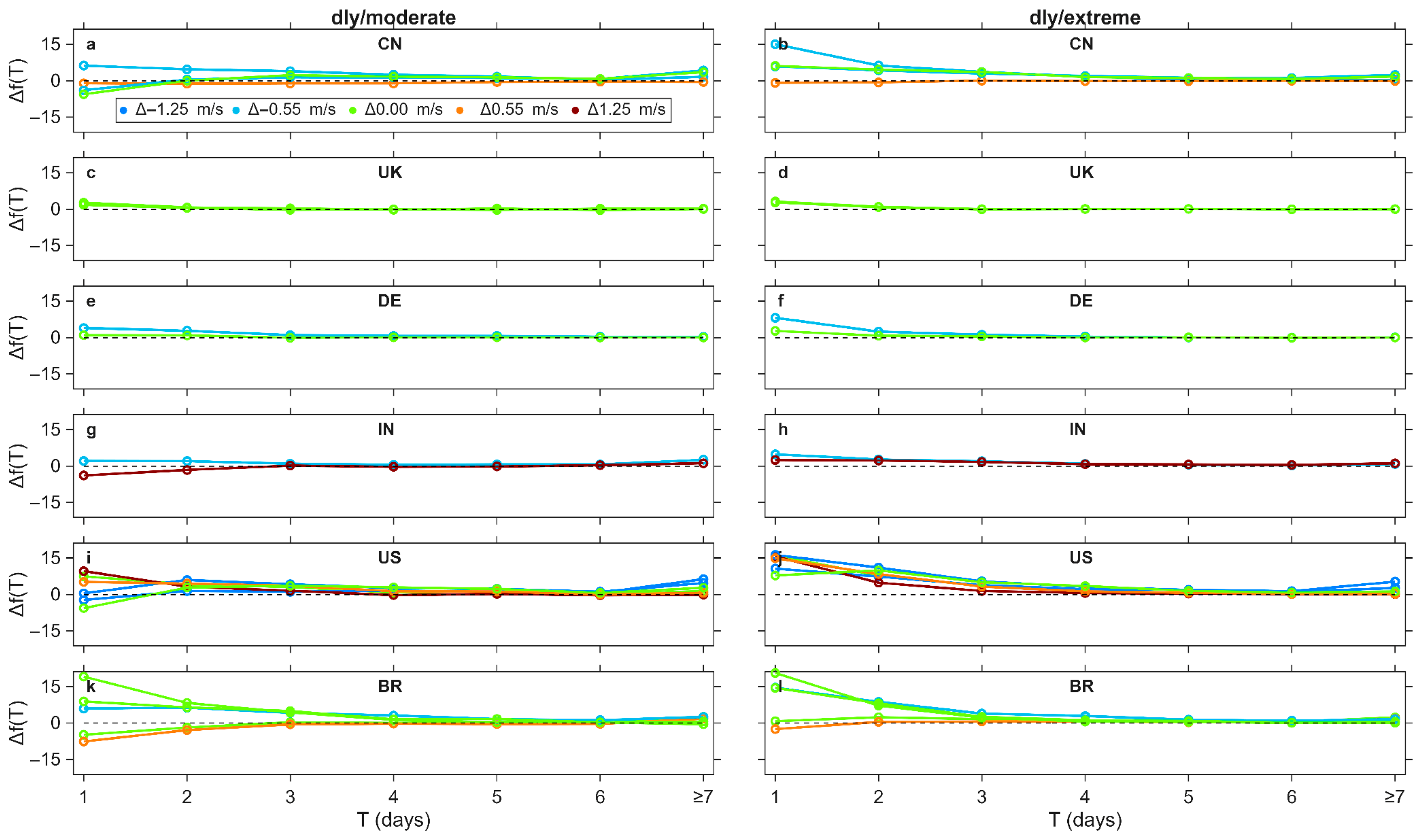
The scenarios have a pronounced impact on the frequency of different wind energy drought duration classes. Figure 6 illustrates the change in frequency of T (Δf(T)) at the daily temporal scale compared to the BASELINE scenario. The magnitude of these changes varies considerably among EEZs. Overall, the findings indicate that the extent of the effects of wind turbine technology, wake effect intensity, and availability on wind energy drought characteristics is highly region-specific.

The most significant change in any wind energy drought class is observed in China, where the number of moderate droughts lasting two days increases by 4.6 per year under the OLD scenario. In India, the OLD scenario results in a substantial rise in very long moderate wind energy droughts (≥7 days), while the frequency of shorter droughts declines. This suggests that, under the OLD scenario, multiple shorter drought events are increasingly merging into prolonged drought periods. In contrast, under the MORE scenario, only the frequency of short-duration droughts increases. In Brazil, the OLD scenario is associated with a similar increase across all duration classes. The lowest Δf(T) value is −3.2 per year for one-day moderate wind energy droughts in the EEZ of the USA under the LESS scenario.

For extreme wind energy droughts, the changes are predominantly confined to shorter-duration events, while long-duration droughts are minimally affected by the different scenarios, likely due to their overall rarity. Overall, estimated changes in extreme droughts should be interpreted with caution, as small sample sizes lead to increased statistical uncertainty.

3.4. Impact of Spatial Diversification on Wind Energy Droughts

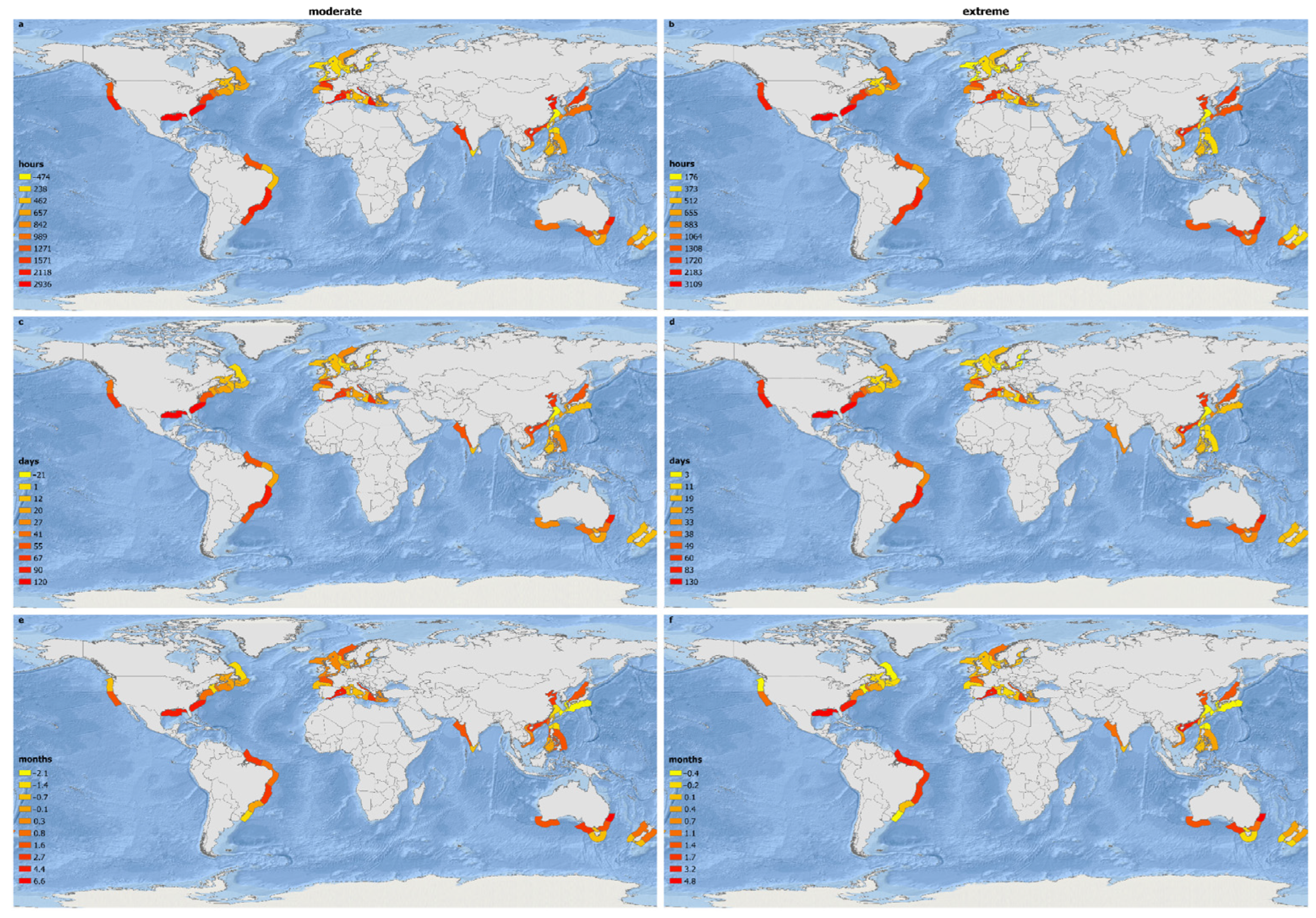
In general, wind energy droughts are much more pronounced in MEs within EEZs than in the EEZs as a whole. Figure 7 presents ΔN for 61 MEs compared to their respective entire EEZs. For moderate wind energy droughts at the hourly time scale, ΔN is positive in 60 out of 61 evaluated MEs.

The highest ΔN value is observed in the “Northern Gulf of Mexico”, with an increase of 2936 h per year. For extreme wind energy droughts, all ΔN values are positive, indicating a consistent increase across all regions. On a daily time scale, there are also hardly any MEs that show negative ΔN values.

These results clearly indicate that, with respect to wind energy droughts, situating individual offshore wind turbines within a single subregion offers no benefit. In contrast, distributing wind turbines across multiple subregions significantly reduces wind energy droughts. Moreover, the magnitude of the differences between subregions and the entire EEZ has a substantially greater influence on wind energy droughts than technological factors such as turbine design, wake effects, and availability.

Spatial diversification also has some disadvantages. These include increased costs for transmission infrastructure, grid connection, and maintenance due to longer distances and more complex logistics. In addition, project development and approval procedures become more difficult and costly when multiple sites located far apart from each other are involved. In addition, spatial diversification may lead to a reduction in mean annual wind energy yields.

The “East China Sea” represents a notable exception to the general benefits of spatial diversification. In this case, ΔN is negative at −474 h per year, indicating fewer wind energy droughts when offshore wind turbines are concentrated within the “East China Sea” compared to aggregation across the entire Chinese EEZ. This negative diversification effect cannot be explained by a mean wind speed that is 0.7 m/s higher than the EEZ-wide average alone, but is instead driven by differences in the temporal persistence of low-wind speed events. While droughts in the “East China Sea” are relatively short-lived, other parts of the Chinese EEZ exhibit more persistent low-wind speed conditions, such that aggregation across the full EEZ increases drought occurrence. This highlights that spatial diversification is only effective when it exploits asynchronous low-wind speed variability across regions. The benefits of spatial diversification are substantially diminished when considering wind energy droughts at the monthly time scale. For moderate monthly wind energy droughts, there are 24 MEs in which the ΔN values are negative, and for extreme monthly droughts, this is the case for 18 EEZs.

The reduction in the effectiveness of spatial diversification at monthly time scales is consistent with the influence of large-scale atmospheric circulation patterns. Persistent blocking events, monsoon systems, or other slowly evolving climate modes often lead to spatially coherent low wind speed conditions over entire EEZs for extended periods. While the present study does not explicitly attribute individual drought events to specific climate modes, it highlights the importance of such large-scale drivers for understanding prolonged offshore wind energy droughts.

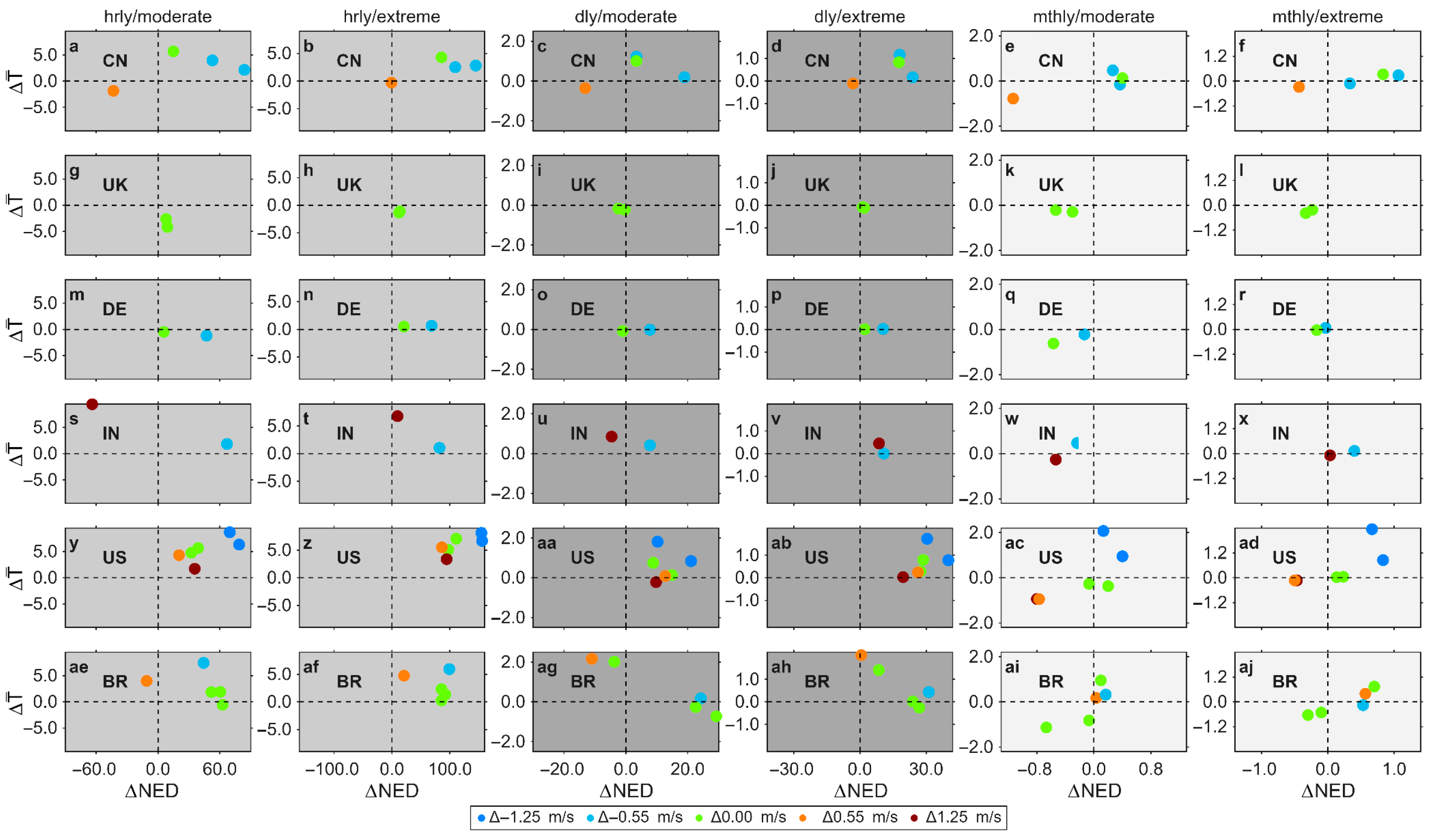
Figure 8 offers a detailed examination of wind energy drought characteristics by presenting Δ$\overline{T}$ and ΔNED for MEs of six EEZs across all combinations of temporal scale and drought intensity. The sub-figures include four quadrants that show the differences in NED and $\overline{T}$ of the MEs with respect to the results of the entire EEZ. The results demonstrate that changes in NED and $\overline{T}$ are largely determined by the specific EEZ, ME, temporal resolution, and drought intensity considered.

For example, in the USA, both $\overline{T}$ and NED are higher for all six MEs than for the EEZ as a whole when considering wind energy droughts on an hourly scale. There are instances where the trends in NED and $\overline{T}$ diverge. Conversely, in the UK’s EEZ, both MEs exhibit higher NED but lower $\overline{T}$ values compared to the overall EEZ.

The figure also displays the difference in ${\overline{U}}_{\mathrm{E}\mathrm{R}\mathrm{A}\mathrm{5,150}\mathrm{m}}$ (${\mathsf{\Delta }\overline{U}}_{\mathrm{E}\mathrm{R}\mathrm{A}\mathrm{5,150}\mathrm{m}}$) for each ME relative to its entire EEZ. At hourly and daily scales, even MEs with positive wind speed differences frequently have positive $\overline{T}$ and NED values. This indicates that spatial diversification, including low and high wind speed regions, can be advantageous compared to only siting wind turbines in a small high wind speed region. However, this relationship does not hold for monthly wind energy droughts.

Figure 9 presents Δf(T) at the daily temporal scale for MEs compared to their respective entire EEZs. The changes in f(T) are often substantial and highly region-specific. For example, in the Brazilian ME “Rio Grande”, the number of one-day moderate wind energy droughts is 19.1 per year, higher than in the EEZ as a whole. However, Δf(T) for one-day moderate droughts in the ME “Northeastern Brazil” is −7.6 per year. Conversely, the frequency of droughts lasting seven days or more increases by 1.0 per year in “Northeastern Brazil”. The smallest differences in f(T) between MEs and their total EEZ occur in the two UK MEs, where values for short-duration droughts are only slightly positive. Overall, the pronounced spatial variability in the impact of wind energy droughts highlights the necessity of considering regional characteristics in wind turbine siting to effectively mitigate wind energy drought risks.

4. Conclusions

The presented global, multi-scale approach to offshore wind energy droughts provides a consistent basis for quantifying the mitigation potential of supply-side interventions. A key quantitative insight is that spatial diversification across multiple sub-regions emerges as the most effective strategy for mitigating offshore wind energy droughts of EEZs. This effect is most pronounced at hourly and daily time scales, while its benefits are substantially reduced at monthly resolution, highlighting clear scale-dependent limitations of spatial diversification. Despite these advantages, spatial diversification must be balanced against potential drawbacks, including increased infrastructure costs, grid expansion requirements, lower mean annual energy yields, and impacts on the marine environment.

Beyond spatial diversification, this study demonstrates that advances in wind turbine technology, as well as reductions in wake losses and downtime, can further mitigate wind energy droughts, although their overall effectiveness is lower than that of spatial diversification.

This analysis further reveals that the statistical properties of the capacity factor and the resulting characterization of wind energy droughts depend strongly on the chosen temporal scale. Results obtained at one temporal resolution cannot be directly transferred to another, as hourly, daily, and monthly droughts are governed by different physical drivers and have fundamentally different implications for offshore wind integration and power system operation. Consequently, the effectiveness of mitigation measures is inherently time-scale dependent.

The results further indicate that at longer time scales, the investigated supply-side mitigation measures must be complemented by system-level solutions to ensure power system adequacy and reliability. In particular, prolonged offshore wind energy droughts at monthly resolution require long-duration energy storage, dispatchable low-carbon backup capacity, or enhanced interregional transmission. Policymakers should therefore distinguish between short-term variability at hourly and daily scales, which can be effectively mitigated through diversified offshore wind turbine siting, and persistent low-wind periods at monthly scales, which require structural investments in system flexibility and adequacy. Further research is warranted to assess how these supply-side mitigation strategies interact with broader system-level and demand-side measures, such as energy storage, sector coupling, hybrid renewable systems, and transmission expansion. In this context, the results of the present study can serve as a complementary input to integrated energy system models and long-term planning studies, thereby supporting more robust and resilient offshore wind deployment strategies.