Energy as a Lingering Barrier: Identifying Persistent Challenges in China’s Carbon Reduction and Pollution Abatement via Explainable Machine Learning

Abstract

Persistent energy system inertia continues to hinder China’s carbon reduction progress despite global decarbonization trends. This study develops an explainable machine learning framework to dissect energy-related emission drivers through 14 secondary indicators spanning energy structure, industrial dynamics, social factors, and economic factors. Leveraging panel data from 260 Chinese cities (2000–2023), we conduct comparative analysis of six ML models and identify XGBoost as optimal for capturing nonlinear emission patterns. SHAP value decomposition and feature importance reveals that total energy consumption and energy consumption intensity remain the dominant contributors to carbon and pollution emissions, while the secondary industry still emerges as a critical driver. Our research establishes an actionable framework to identify drivers of carbon mitigation and pollution reduction, analyze their mechanisms, and support policymakers in optimizing policy implementation amid energy transition.

1. Introduction

Over the past four decades, global energy consumption has more than doubled, with China accounting for over a quarter of this total [1,2]. The persistent dominance of fossil fuels drives significant carbon and pollutant emissions, undermining ecological and human health [3]. Cities, as concentrated hubs of energy use and emissions, are critical arenas for energy transition and clean energy adoption. Their success in reducing emissions directly determines national low-carbon goals, yet the drivers at the urban scale are complex, involving industrial structure, energy consumption, and socio-economic factors [4]. Clarifying these mechanisms—particularly the role of energy transition dynamics—is essential for effective governance.

Regarding the research objects, relevant studies mainly focus on the national level [5,6,7], provincial level [8,9], the Yangtze River Delta region [10], the Beijing–Tianjin–Hebei urban agglomeration [11], the Yangtze River Basin [12], and the Yellow River Basin [13]. Scholarly investigation into the drivers of carbon and pollutant emissions has proliferated, yielding significant insights. Research has consistently identified a core set of contributing factors, including industrial structure [14], energy consumption patterns and intensity [15,16,17], economic growth [18,19,20], and population scale. Methodologically, this body of work has largely relied on two approaches. The first encompasses decomposition analysis techniques, such as Structural Decomposition Analysis (SDA) and Index Decomposition Analysis (IDA), which are valued for isolating the structural and intensity effects of different factors [21]. The second includes efficiency evaluation and econometric models, notably Data Envelopment Analysis (DEA) for performance benchmarking [22,23] and the STIRPAT model for assessing anthropogenic impacts [24,25,26]. However, these traditional methods possess inherent constraints. Decomposition analyses often depend on restrictive linear assumptions or static input–output tables, struggling to capture the complex, non-linear interactions between drivers [27]. Similarly, econometric models like STIRPAT can face convergence issues and diminished explanatory power when handling high-dimensional, multi-factor datasets, limiting their ability to quantify synergistic effects.

The advent of machine learning (ML) has introduced powerful new tools for analyzing complex environmental systems, offering superior capacity to model non-linear relationships and handle large-scale data [28,29,30,31]. Studies have effectively employed algorithms such as Random Forest and Long Short-Term Memory (LSTM) networks for predicting carbon emissions and pollutant concentrations [32,33]. Among these, ensemble models like XGBoost are particularly favored for their robustness and predictive accuracy in factor mining applications [34]. Nevertheless, the “black-box” nature of many advanced ML models historically impeded causal interpretation, creating a gap between prediction and explanation. This is where the rapidly developing field of explainable machine learning (XAI) becomes critical. XAI techniques, including SHAP (SHapley Additive exPlanations) and other post hoc interpretation frameworks, enable researchers to peer inside these complex models. They allow for the quantification of variable importance, the visualization of non-linear effect patterns, and the assessment of interaction effects, thereby revealing the underlying drivers and mechanisms [35].

Despite these advances, significant gaps remain. First, most studies focus on national or regional levels, with limited analysis at the city scale—where energy transition pressures are most acute. Moreover, research often treats carbon and pollutant emissions separately, rather than examining their synergistic mitigation within an energy transition framework. Second, while explainable ML shows promise, its application in China to unravel the complex, nonlinear drivers of urban emission reduction—particularly those tied to clean energy penetration and energy structure optimization—remains underexplored. This study addresses these gaps by applying an explainable ML approach to analyze the integrated drivers of pollution and carbon reduction in Chinese cities, thereby providing a nuanced, data-driven perspective to inform targeted urban energy transition policies.

The structure of this paper is arranged as follows: the introduction section outlines the research background and related literature; the materials and methods section explains the data used and the research ideas; then the experimental results are analyzed; the discussion section further elaborates on the research findings; and finally, the full text is summarized and conclusions are drawn.

2. Materials and Methods

2.1. Data Sources and Variable Descriptions

Based on the availability and completeness of data, this study selected partial data from 260 cities in China from 2000 to 2023. The PM_2.5 concentration data were obtained from the V5.GL.04 estimation results released by the Atmospheric Composition Analysis Group at Washington University in St. Louis. And CO₂ data were sourced from the China Emission Accounts and Datasets (CEDS). Other data were derived from the China Urban and Rural Statistical Yearbook, among other sources. The missing values were filled using the moving average method.

Table 1 presents the descriptive statistical results of the variables involved in the study, covering five categories: independent variables, energy contributors, social contributors, economic contributors and industrial contributors. Among social contributors, population size influences emissions and pollution through domestic energy consumption and infrastructure demands. Urbanization has a phased impact (emissions increase in the initial stage, and in the mature stage, emissions may be reduced due to economies of scale and enhanced environmental awareness). Population density has a two-way effect through spatial efficiency (high density reduces per capita energy consumption but may exacerbate pollution aggregation). Green space, as a core component of the natural ecosystem, directly absorbs CO₂ through photosynthesis of vegetation, playing a “carbon sink” function. At the same time, it reduces the PM_2.5 concentration in the air through leaf adsorption and dust-retention, directly reducing pollutants. In economic contributors, GDP reflects the relationship between economic scale and emissions. GDP per capita reflects the impact of residents’ consumption capacity on consumption-side emissions. The total number of green patent authorizations promotes emission reduction in the production process of enterprises and the low carbonization of industries at the economic level. FDI has a two-way impact on carbon reduction and pollution abatement through technology spillover and industrial transfer. Among industrial contributors, the secondary industry (especially heavy industry) is the core source of carbon emissions and pollution. The primary industry generates emissions and pollution due to agricultural machinery energy consumption, fertilizer use, and straw burning. The tertiary industry, with low energy consumption and emission intensity, helps to reduce the overall emission intensity as its proportion increases. In terms of energy contributors, total energy consumption directly determines the total amount of emissions and pollution. Night-light data indirectly reflects the spatial distribution of energy consumption and emissions. Energy consumption intensity reflects the impact of energy use efficiency on carbon reduction and pollution abatement.

Table 1. Variable Descriptions.

Category	Variables	Abbreviation	Mean	SD	25%	75%
Independent variables	CO2	CO2	36.46	39.78	12.99	44.85
	PM2.5	PM2.5	46.53	15.17	35.32	55.81
Energy contributors	Total energy consumption	TEC	131,417	118,339	50,746	167,771
	Nighttime Light Data	NL	7.48	8.81	1.87	9.36
	Energy Consumption Intensity	ECI	1.04	0.81	0.57	1.28
Social contributors	Population	Pop	497.75	385.09	253	625.5
	Urbanization	Urb	0.51	0.17	0.39	0.62
	Population Density	Pop den	534.43	613.31	209.04	669
	Per capita Green space	PCUGS	11.42	5.09	8.21	14.14
Economic contributors	GDP	GDP	2163	3570	560	2256
	Per capital GDP	GDP per	37,434	30,341	17,475	52,377
	Total Green Patent Authorization	TGPA	238	794	9	125
	Foreign Direct Investment	FDI	903	2116	67.76	783
Industrial contributors	Added Value of the Primary Industry	PI	149	119	67	200
	Added Value of the Secondary Industry	SI	969	1300	262	1089
	Added Value of the Tertiary Industry	TI	1045	2351	195	913

Among the independent variables, the mean of CO₂ emissions is 36.46, with a standard deviation of 39.78, indicating a high degree of data dispersion. The mean of PM_2.5 is 46.53, with relatively less fluctuation compared to CO₂ emissions (SD = 15.17). In terms of social contributors, the mean of the population (Pop) is 497.75, and the mean of the urbanization rate (Urb) is 0.51, representing a medium level of urbanization. Variables such as population density (Pop den) also exhibit their respective data distribution characteristics. Regarding economic contributors, the mean of GDP is 2163.93, but the large standard deviation of 3570.51 indicates significant differences in economic scale among the samples. Variables such as GDP per capita (GDP per) and the total number of green patent authorizations (TGPA) reflect the economic development and innovation investment. For industrial contributors, the means of the added values of the primary, secondary, and tertiary industries (PI, SI, TI) reflect the basic pattern of the industrial structure. The large standard deviations of the added values of the secondary and tertiary industries suggest obvious differences in industrial scale. In the energy factor category, the mean of the total energy consumption (TEC) is 131,417.27, with a standard deviation of over 110,000, highlighting prominent differences in energy consumption. Variables such as night-light data (NL) and energy consumption intensity (ECI) help to depict characteristics related to energy utilization. These statistics provide basic data support for the subsequent exploration of the relationships and action mechanisms among various contributors, presenting the overall distribution and dispersion of the samples across multi-dimensional indicators.

2.2. Carbon Emission and Pollution Emission Intensity Indicator

To characterize the overall performance of urban carbon reduction and pollution abatement, we construct an Index of carbon emission and pollution emission intensity indicator (CPEII), integrating the emission efficiencies of multiple pollutants and greenhouse gases into a single indicator. The calculation formula is presented as Equation (1):

$$R_{\mathrm{I}\mathrm{P}\mathrm{C}}={\sum }_{i=1}^2{E}_i\times q_i$$

(1)

In which $R_{\mathrm{I}\mathrm{P}\mathrm{C}}$ (MT) represents the final index of carbon and pollution intensity, where the higher the value, the stronger the intensity. $E_i$ represents the emission intensity of the i-th pollutant, and $q_i$ represents the weight of the i-th pollutant.

2.3. Machine Learning Methods and Assessment Indicators

2.3.1. XGBoost

XGBoost is a machine learning algorithm based on Gradient Boosting Decision Trees (GBDT) [36]. Its core idea is to form a strong classifier by gradually constructing multiple weak classifiers. In each iteration, the algorithm fits the residuals of the previous model to enhance the overall predictive performance. The Boosting strategy corrects the errors in each iteration, which allows the model to achieve higher predictive accuracy with fewer computational resources when dealing with high-dimensional data and complex tasks, and effectively avoids overfitting. Compared to traditional GBDT algorithms, XGBoost introduces regularization terms, parallel computing, and caching mechanisms, which significantly improve the model’s predictive accuracy, training speed, and resistance to overfitting. These advantages make the XGBoost algorithm widely used in solving regression prediction problems. The objective function of XGBoost is presented as Equation (2):

$$Objective={\sum }_{i=1}^{n}loss\left(y_i,{\widehat{y}}_i\right)+{\sum }_{k=1}^k\Omega \left(f_k\right)$$

(2)

$loss\left(y_i,{\widehat{y}}_i\right)$ is the loss function, which measures the difference between the true value $y_i$ and the predicted value ${\widehat{y}}_i$, and $\Omega \left(f_k\right)$ is the regularization term of the model, used to control model complexity and prevent overfitting.

2.3.2. GBDT

GBDT (Gradient Boosting Decision Tree) is a commonly used machine learning algorithm that builds a strong learner by iteratively training a series of decision trees [37,38]. It is a powerful ensemble algorithm widely applied in both regression and classification tasks. The algorithm starts with a simple base model, usually a basic predictor that provides an initial prediction, such as the average value of target variables for regression tasks. In each subsequent iteration, it focuses on correcting the errors made by the current ensemble model. Specifically, it calculates the negative gradient of the loss function with respect to the existing predictions, which serves as pseudo-residuals to quantify the discrepancies between the actual target values and the model’s outputs. A new decision tree is then trained to fit these pseudo-residuals, aiming to compensate for the prior prediction errors. Once trained, this new tree is integrated into the ensemble model, and the process repeats iteratively. The iteration stops when the number of trees reaches a predefined threshold or the model’s prediction error no longer decreases significantly. The final GBDT model is the sum of the predicted values of all decision trees.

2.3.3. Random Forest

Random Forest is a powerful machine learning algorithm that combines multiple decision trees to improve the accuracy and generalization of predictions [39,40]. It is widely used in various fields due to its ability to handle high-dimensional data and complex relationships.

The key idea behind Random Forest is to build an ensemble of decision trees, where each tree is trained on a random subset of the data and a random subset of the features. This randomization helps to reduce overfitting and increase the diversity of the ensemble.

The prediction of a Random Forest is obtained by averaging the predictions of all the individual decision trees. Mathematically, for a given input x, the prediction of the i-th tree is denoted as f_i(x), and the final prediction of the Random Forest is $f\left(x\right)={\displaystyle \frac{1}{T}}\sum _{i=1}^T{f}_i\left(x\right)$.

Random Forest has several advantages over individual decision trees. It is less prone to overfitting, can handle missing values and categorical features, and provides an estimate of the importance of each feature.

2.3.4. LightGBM

LightGBM is a gradient boosting framework that is designed to be more efficient and scalable than traditional gradient boosting algorithms [41]. It uses a novel histogram-based algorithm to speed up the training process and reduce memory usage. The main idea behind LightGBM is to split the data into small subsets based on the values of the features and then build a decision tree for each subset. The decision trees are grown in a way that minimizes the loss function, which is typically the mean squared error or the cross-entropy loss.

Mathematically, the LightGBM algorithm can be described as follows: Let X be the input data, y be the target variable, and F be the set of features. The algorithm starts by initializing the model with a constant value $f_0\left(x\right)=\overline{y},$ where $\overline{y}$ is the mean of the target variable. Then, for each iteration m = 1, 2,…M, the following steps are performed: (1) Compute the gradients of the loss function with respect to the current model. (2) Group the data points into bins based on the values of the features. (3) Compute the gradients for each bin. (4) Build a decision tree to approximate the gradients of the loss function. (5) Update the model by adding the predictions of the decision tree. The final model is a weighted combination of the decision trees, where the weights are determined by the performance of the trees on the training data.

2.3.5. AdaBoost

AdaBoost (Adaptive Boosting) is a popular machine learning algorithm used for classification and regression tasks [42]. It is based on the idea of boosting, which combines multiple weak learners (simple models) to create a strong learner (a more accurate and robust model). The key idea behind AdaBoost is to iteratively train a sequence of weak learners, each one focusing on the examples that were misclassified by the previous learner. At each iteration, the algorithm assigns weights to the training examples, giving more weight to the misclassified ones. This way, the subsequent weak learners are forced to pay more attention to the difficult examples and improve the overall performance of the ensemble.

The final classifier is a weighted combination of the weak learners, where the weights are determined by their performance on the training data. AdaBoost has several advantages, including its ability to handle noisy data, its high accuracy, and its relatively low computational complexity. However, it can also be sensitive to outliers and may overfit the training data if not properly regularized.

2.3.6. Lasso

Lasso (Least Absolute Shrinkage and Selection Operator) is a regression analysis method that can be used for variable selection and regularization [43]. It is a modification of the ordinary least squares regression method that adds a penalty term to the objective function to encourage the coefficients of the predictor variables to be small. The Lasso regression model can be formulated as Equation (3):

$${\mathrm{m}\mathrm{i}\mathrm{n}}_{\beta }{\displaystyle \frac{1}{2n}}\left|\left|y-X\beta {\left|\right|}_2^2+\lambda \right|\right|{\beta \left|\right|}_1$$

(3)

where y is the response variable, X is the predictor matrix, β is the vector of regression coefficients, n is the number of observations, and λ is the regularization parameter that controls the strength of the penalty. The first term in the objective function is the ordinary least squares loss function, which measures the goodness of fit of the model. The second term is the Lasso penalty term, which shrinks the coefficients towards zero and selects a subset of the predictor variables.

The Lasso penalty has the effect of forcing some of the coefficients to be exactly zero, which results in a sparse model with only a few predictor variables. This can be useful for variable selection, as it allows us to identify the most important predictor variables and remove the unimportant ones. In addition, the Lasso penalty can also improve the generalization performance of the model by reducing overfitting.

2.3.7. Assessment Indicator

This study employs five validated performance evaluation metrics: Mean Absolute Error (MAE) (Equation (4)), Mean Squared Error (MSE) (Equation (5)), Mean Absolute Percentage Error (MAPE) (Equation (7)), Root Mean Square Error (RMSE) (Equation (6)) and the Coefficient of Determination (R²) (Equation (8)) to assess the predictive performance of six machine learning algorithms.

$$\mathrm{M}\mathrm{A}\mathrm{E}={\displaystyle \frac{1}{n}}{\sum }_{i=1}^n\left|y_i-{\widehat{y}}_i\right|$$

(4)

$$\mathrm{M}\mathrm{S}\mathrm{E}={\displaystyle \frac{1}{n}}{\sum }_{i=1}^n\hspace{1em}{\left(y_i-{\widehat{y}}_i\right)}^2$$

(5)

$$\mathrm{R}\mathrm{M}\mathrm{S}\mathrm{E}=\sqrt{\mathrm{M}\mathrm{S}\mathrm{E}}$$

(6)

$$\mathrm{M}\mathrm{A}\mathrm{P}\mathrm{E}={\displaystyle \frac{1}{n}}{\sum }_{i=1}^n\left|{\displaystyle \frac{\left(y_i-{\widehat{y}}_i\right)}{{\widehat{y}}_i}}\right|\ast 100\%$$

(7)

$${\mathrm{R}}^2=1-{\displaystyle \frac{\sum _{i=1}^n{\left(y_i-{\widehat{y}}_i\right)}^2}{\sum _{i=1}^n{\left(y_i-\overline{f}\left(x_i\right)\right)}^2}}$$

(8)

Here, n is the number of samples, $y_i$ is the actual value of the carbon reduction and pollution abatement intensity, ${\widehat{y}}_i$ is the predicted value of the carbon reduction and pollution abatement intensity, and $\overline{f}\left(x_i\right)$ is the average value of the carbon reduction and pollution abatement intensity. The higher the values of Mean Squared Error (MSE) and Mean Absolute Percentage Error (MAPE), the greater the prediction error. The Coefficient of Determination (R²) ranges from 0 to 1, with higher values indicating a better model fit.

2.4. Explainable Methods

2.4.1. SHAP Values Algorism

Although machine learning methods can accurately identify the factors of carbon reduction and pollution abatement, they are essentially “black box” models, making it difficult to intuitively reflect the importance and direction of the impact of each factor on carbon reduction and pollution abatement. The SHAP (SHapley Additive exPlanations) value algorithm, proposed by Lundberg [44], is an effective method for explaining machine learning prediction results. This algorithm is based on the concept of Shapley values in cooperative game theory, considering the contribution degree of influencing contributors, and can quantify the importance and direction of the impact of each factor on carbon reduction and pollution abatement. It can be used to visualize the prediction results of the machine learning prediction model XGBoost.

Assume the set of contributors affecting carbon reduction and pollution abatement is $\{x_1,x_2,\dots ,x_p\}$; S is a subset that does not include the factor xi, |S| is the size of the subset; f(S) is the model output corresponding to the subset S; $f\left(S\cup \left\{x_i\right\}\right)$ is the output result after the factor x_i is added to the subset S. Therefore, the SHAP value calculation formula for the factor x_i is as Equation (9):

$$SHAP\left(x_i\right)={\sum }_{S\subseteq \left\{x_1,x_2,\dots ,x_p\right\}\backslash \left\{x_i\right\}}{\displaystyle \frac{\left|S\right|!\left(p-\left|S\right|-1\right)!}{p!}}\left[f\left(S\cup \left\{x_i\right\}\right)-f\left(S\right)\right]$$

(9)

From this, it can be seen that the SHAP value is essentially the weighted average of the changes in model output results before and after the inclusion of the influencing factor x_i, considering all possible combinations of influencing contributors. This method determines the contribution of the influencing factor xi to carbon reduction and pollution abatement, which is highly consistent with the concept of Shapley values in cooperative game theory. The SHAP value interpretation method can accurately identify the main influencing contributors of the synergistic enhancement of carbon reduction and pollution abatement, which is beneficial for providing more efficient and precise decision-making references.

2.4.2. PDP

In addition to the SHAP value theory, the Partial Dependence Plot (PDP) [45] is also a powerful tool for explaining and visualizing how the predictions of machine learning models change with variations in one or more feature values, capable of revealing linear, monotonic, or more complex relationships between features and model predictions. Unlike the locality of SHAP values, PDP analyzes the impact of the target feature on model output by holding other features constant, thereby providing a global understanding of model predictions. This graphical representation method not only helps identify important features in the model but also reveals potential non-linear relationships between features and prediction outcomes. The calculation formula is presented as Equation (10):

$$\widehat{\varphi }(x_1)\equiv {\displaystyle \frac{1}{n}}{\sum }_{i=1}^n\hspace{1em}f(x_1,x_{i2},\cdots ,x_{ip})$$

(10)

Here, $\widehat{\varphi }\left(x_1\right)$ represents the average change in model predictions when the feature $x_1$ is held constant. In the formula, n is the number of samples in the dataset, $f$ is the model’s prediction function, $x_1$ is the specific feature value we are interested in, and $x_1,x_{i2},\cdots ,x_{ip}$ represent the other feature values of the i-th sample in the dataset, excluding $x_1$. For any given value of $x_1$, we can calculate $\widehat{\varphi }\left(x_1\right)$, which represents the average change in the model’s prediction results when $x_1$ varies. Then, we can visualize $(x_1,\widehat{\varphi }(x_1\left)\right)$ as a Partial Dependence Plot (PDP).

3. Results

3.1. Model Comparison Results

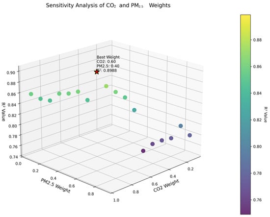
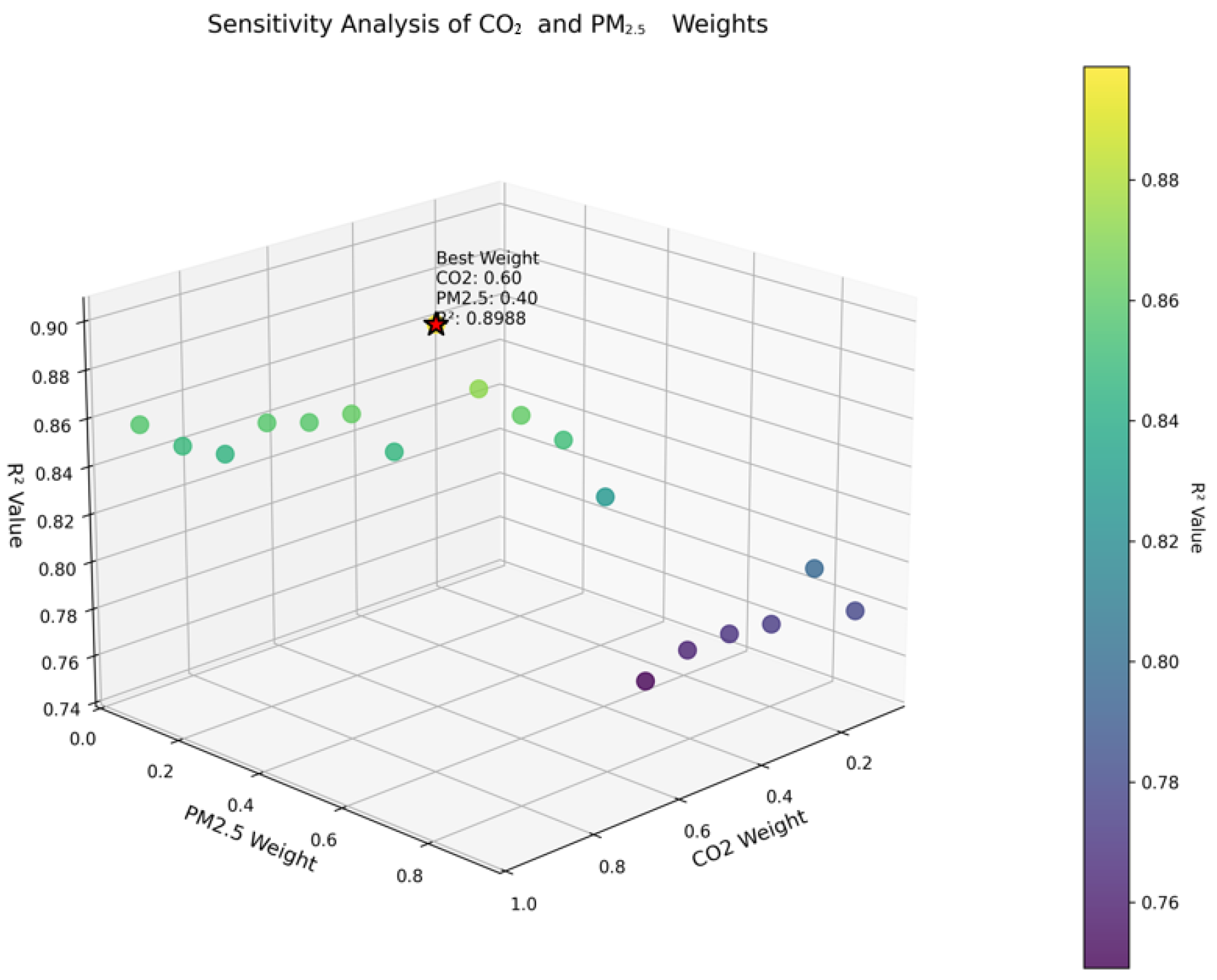
In order to find the best combination weight of PM_2.5 and CO₂ in CPEII, we conducted a sensitivity analysis (Figure 1). Based on multiple parameter adjustments and considering the importance of both contributors, it was found that 0.4 and 0.6 are the optimal parameters for the regression, with 0.4 assigned as the coefficient for PM_2.5 and 0.6 for CO₂.

Figure 1. Sensitivity Analysis (red start means the best point).

In this study, to ensure the effectiveness of model training and the objectivity of evaluation, we first split the collected dataset into a training set and a test set at a ratio of 8:2. Specifically, the training set, accounting for 80% of the dataset, is used for parameter learning and fitting optimization of the model. The test set, which makes up 20% of the dataset, serves as independent validation data to objectively assess the model’s generalization ability on unseen data. To ensure the generalization ability of ML models and avoid overfitting, also minimize potential leakage, stratified 5-fold cross-validation was adopted for the classification task. And grid search was applied to optimize hyperparameters of the target ML models. Based on this data division, we further selected six classic and representative machine-learning models to conduct regression modeling on the pollution-and-carbon-reduction intensity index. All experiments were conducted on a laptop equipped with an Intel Core i5 processor, 16 GB DDR4 RAM, running the Windows 11 64-bit operating system. The core programming environment was Python 3.10.8, with key machine learning (ML) libraries including scikit-learn, pandas and numpy.

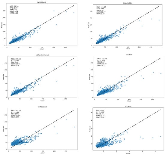
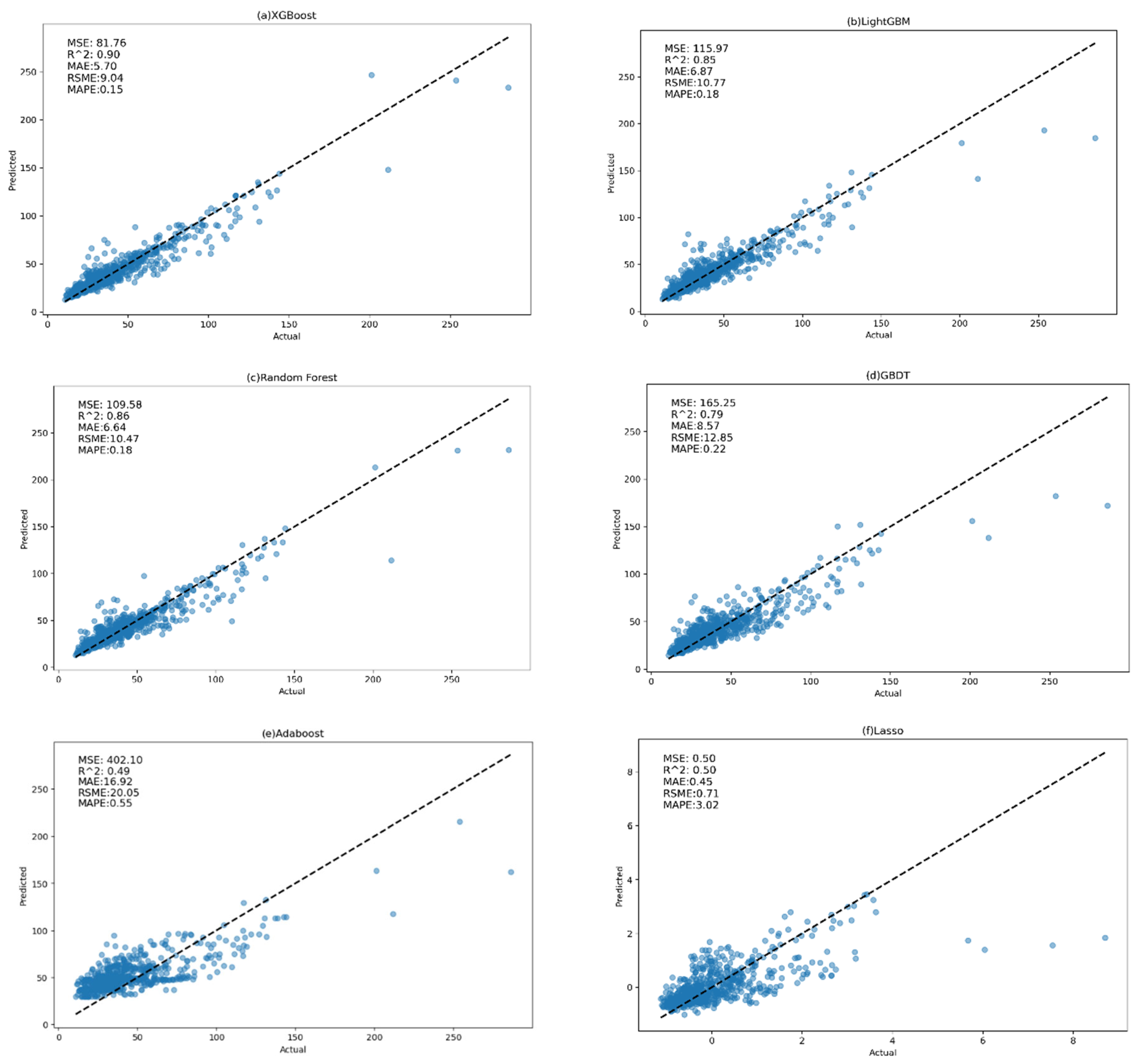
Table 2 presents the comparison results of the models, and Figure 2 illustrates the regression fitting results of the dataset across various models, facilitating an intuitive observation of their performance. In terms of predictive performance, the XGBoost model performed the best, with an MSE of 83.30, an R² coefficient of determination of 0.90, an MAE of 5.75, and an RMSE of 9.13. These metrics all demonstrate XGBoost’s superiority in capturing data patterns and prediction accuracy. Ranking the models based on the R² coefficient, the performance order is XGBoost, RF, LightGBM, GBDT, Lasso (since the algorithm is highly sensitive to data scale, we standardized the data using the z-score method to eliminate the influence of different units), and Adaboost. These findings provide important references for selecting appropriate machine learning models and directions for further research.

Table 2. Model Comparison.

Model	MSE	R2	MAE	RMSE	MAPE
XGBoost	83.30	0.90	5.75	9.13	0.15
GBDT	109.58	0.79	6.64	10.47	0.22
Random Forest	109.58	0.86	6.64	10.47	0.18
LightGBM	115.97	0.85	6.87	10.77	0.18
Adaboost	402.10	0.49	16.92	20.05	0.55
Lasso	0.50	0.50	0.45	0.71	3.02

Figure 2. Model Comparison.

3.2. Analysis of Key Contributors

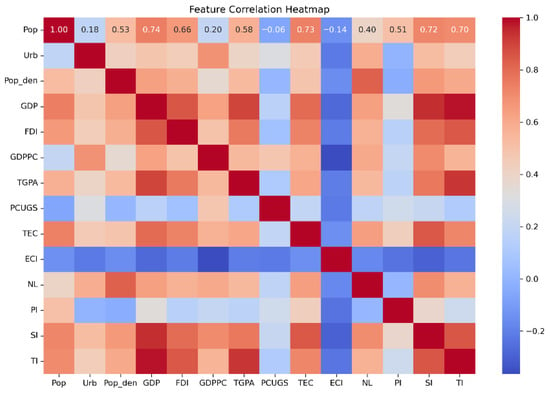
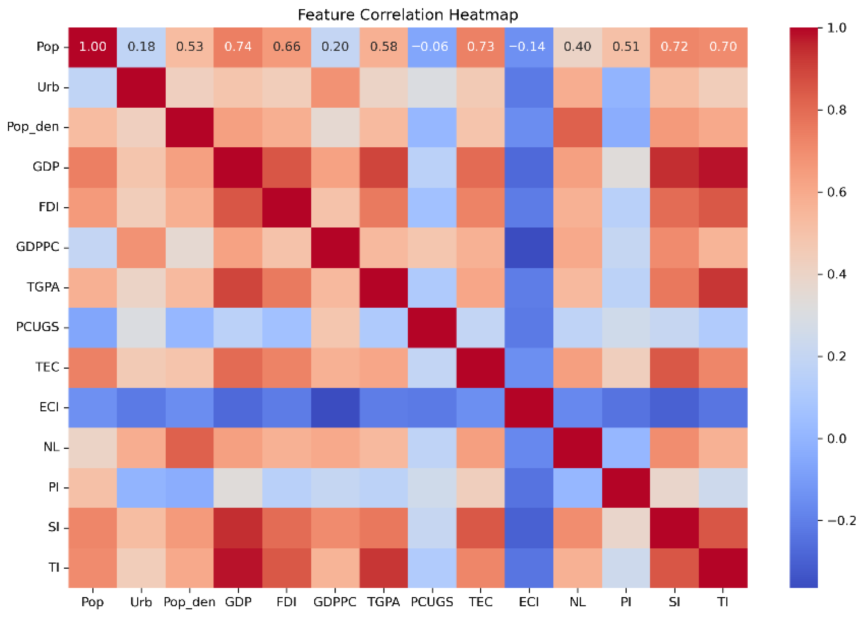
As shown in Figure 3, the heatmap illustrates the Pearson correlation coefficients between the contributors, presenting the correlation matrix of the features involved in the study. The correlation coefficient quantifies the linear relationship between two variables, ranging from −1 (perfect negative correlation) to 1 (perfect positive correlation). The heatmap visually represents these coefficients using color coding, where red indicates positive correlation, blue indicates negative correlation, and the intensity of the color reflects the strength of the correlation. The correlation coefficient between ECI and NL is 0.51, implying that the intensity of nighttime lights is related to energy consumption intensity, which aligns with common understanding, as the intensity of nighttime lights is also an indicator of energy use, with regions having higher nighttime light intensity generally consuming more energy and having a higher level of economic development. Looking at the energy-related contributors, there is a strong correlation with the added value of the secondary industry, which is due to the higher energy consumption associated with the secondary sector. It can be observed that the correlation coefficient between Pop and Pop_den is 0.74, indicating a strong positive correlation between these two features, which is consistent with expectations, as population density, being the number of people per unit area, is typically positively correlated with total population. The correlation coefficient between GDP and TGPA is 0.66, suggesting that regions with higher green patent authorization volumes tend to have higher economic outputs. The correlation coefficient between FDI and GDP is 0.58, indicating that FDI has a positive impact on economic growth.

Figure 3. Feature Correlation Heatmap.

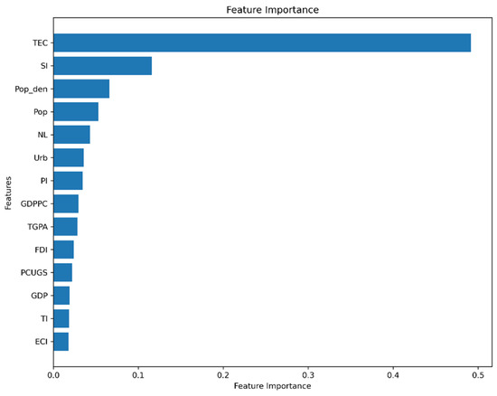
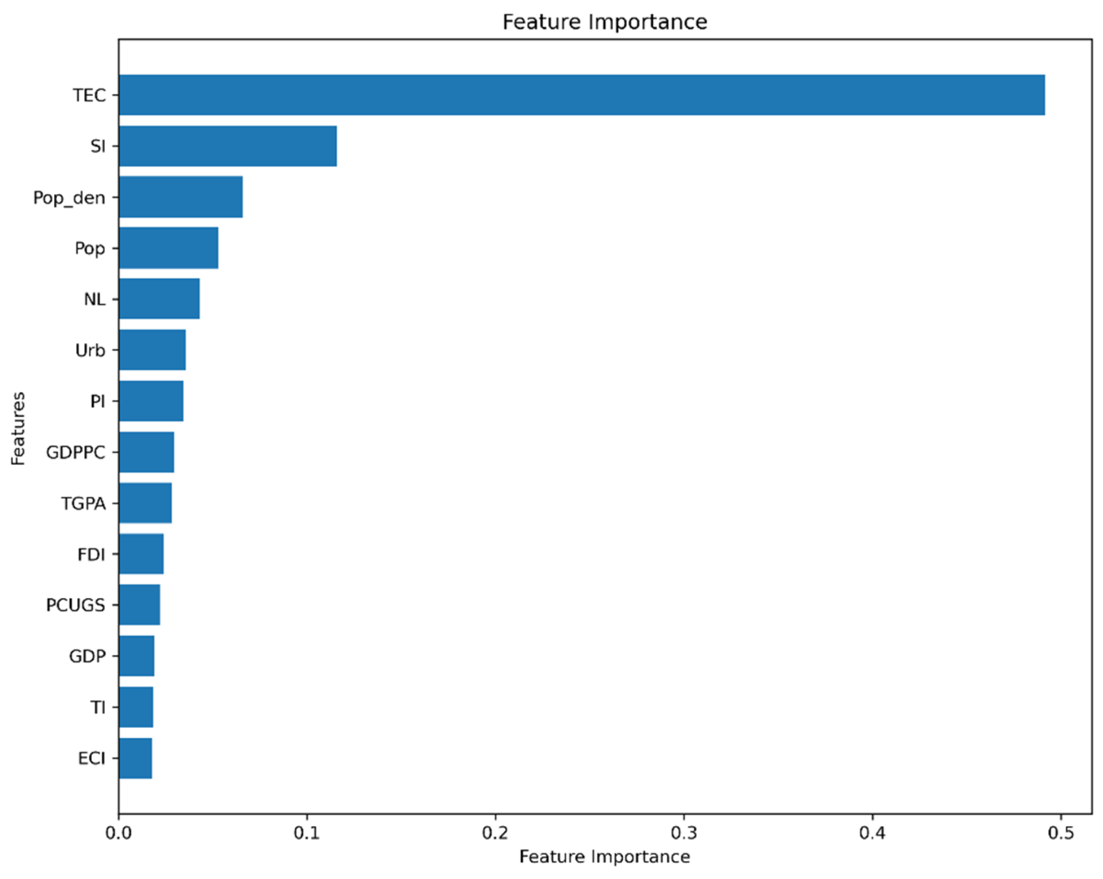
This study analyzes multiple dimensions affecting carbon reduction and pollution abatement. Figure 4 reveals the ranking of feature importance. The research reveals that total energy consumption, the added value of the secondary industry, and population density are the most critical features affecting pollution and carbon emissions, indicating that industrial production and population are the core contributors causing these emissions. Following these are population size, nighttime light intensity, and urbanization rate, which significantly impact pollution and carbon emissions, highlighting the important role of social contributors in the process of carbon reduction and pollution abatement. Subsequently, the added value of the primary industry, per capita GDP, the total number of green patent authorizations, foreign direct investment, and per capita park area also play a role, albeit with relatively lower importance. However, their role in pollution and carbon emissions should not be overlooked, and they can serve as regulatory tools when entering the critical bottleneck phase of carbon reduction and pollution abatement.

Figure 4. Feature importance.

4. Discussion

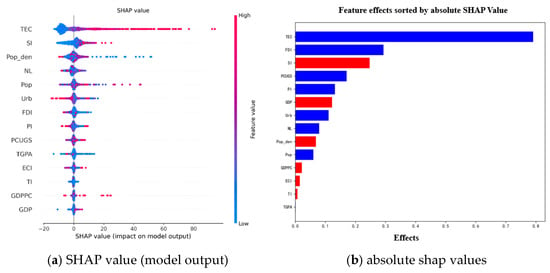
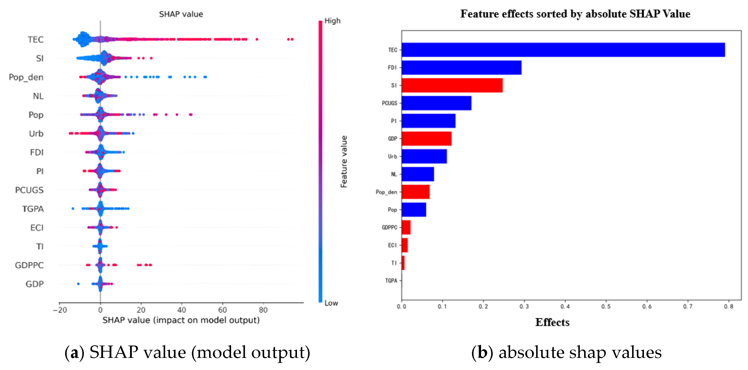
To gain a deeper understanding of the model’s decision-making process, we introduced SHAP values as a supplementary interpretive tool. In Section 3.1, through model comparison, we found that the XGBoost model performed the best, and thus we conducted interpretability analysis based on the XGBoost model. The bees warm plot can display the global distribution of features, ranking features by their average SHAP values while also showing the distribution of feature values and SHAP values. As shown in Figure 5a, the colors indicate whether an instance’s value is positive (red), negative (blue), or in between (purple). The magnitude of the SHAP value represents the impact of the feature on the model’s output, while the color represents the value of the feature. TEC, as the most important feature, has a wide distribution of SHAP values, with high SHAP values mainly concentrated at high TEC values (red), indicating that total energy consumption is the most critical contributor affecting the intensity of carbon emission and pollution emission, and an increase in energy consumption significantly raises the levels of pollution and carbon emissions. The SHAP values for SI are also relatively high and increase with increasing SI values. This may reflect the direct impact of industrial activities on the environment, especially in energy-intensive industries. Additionally, the SHAP values for population density are widely distributed, with high population density (red) associated with higher SHAP values, which may be related to the higher energy consumption and waste generation in densely populated areas. The SHAP values for NL indicate a positive correlation between nighttime light data and the intensity of carbon reduction and pollution abatement. Nighttime light data, often used as a proxy for economic activity and energy consumption, shows a positive correlation with SHAP values, reflecting the relationship between the intensity of economic activity and environmental impact. Although green space area is generally positively correlated with environmental quality, its SHAP values are low, which may be attributed to the limited direct impact of green space area on pollution and carbon emissions. This could be related to the ecological service functions and carbon sequestration capabilities of green spaces, which may not directly reflect in the quantities of pollution and carbon emissions in the short term.

Figure 5. SHAP values.

Figure 5b presents the mean absolute SHAP values for each feature, quantifying their relative importance in driving carbon emission and pollution emission intensity. Table 3 reports the SHAP value signs (positive/negative) and magnitudes, revealing the directional impacts of each factor. Below, we analyze the contributions of energy, social, economic, and industrial factors in detail, with SHAP values indicating that a positive sign corresponds to increased intensity when the feature rises, and vice versa.

Table 3. The SHAP values of the determinants.

Category	Variable	Absolute SHAP Value	Effects	Sign
Social contributors	Population	2.67	0.3228	Positive
	Urbanization Rate	1.15	−0.2152	Negative
	Population Density	2.05	0.0822	Positive
	Per Capita Green Space Area	0.88	−0.1841	Negative
Economic contributors	GDP	0.55	0.0473	Positive
	Per Capita GDP	0.41	0.1044	Positive
	Green Patent Authorization Volume	0.82	0.1166	Positive
	Foreign Direct Investment	1.41	−0.2429	Negative
Industrial contributors	Added Value of the Primary Industry	1.40	−0.1963	Negative
	Added Value of the Secondary Industry	4.34	0.2289	Positive
	Added Value of the Tertiary Industry	0.36	−0.0076	Negative
Energy contributors	Total Energy Consumption	9.79	−0.8346	Negative
	Nighttime Light Data	1.35	−0.1511	Negative
	Energy Consumption Intensity	0.52	−0.0520	Negative

Energy Factors: Total energy consumption, energy intensity, and nighttime light data all exhibit negative effects. However, based on an examination of the SHAP values for individual samples and inferences drawn from Figure 5a, it is possible that some high-energy-consuming samples are often accompanied by structural optimization, such as renewable energy substitution or an increase in the proportion of high value-added industries. Additionally, due to the extensive geographical and temporal scope of this study, there are significant variations in the impacts across different regions and time periods, necessitating more in-depth and detailed research.

Industrial Factors: Secondary industry value-added dominates all factors with the highest mean absolute SHAP value, confirming its central role in emissions. Primary industry value-added shows a negative SHAP, primarily due to its low energy intensity (e.g., agriculture relies more on labor than fossil fuels). Tertiary industry value-added also has a negative impact, differing from primary industry by being service-oriented (e.g., finance, education) with minimal direct energy consumption.

Social Factors: Population exerts the strongest positive influence among social factors, consistent with urban metabolism theory linking population size to aggregate resource consumption and emissions. Urbanization rate follows with a positive but weaker impact, likely due to increased energy demand from expanded infrastructure. Notably, population density shows a negative SHAP value, suggesting that compact urban development may mitigate emissions through agglomeration economies (e.g., reduced transportation costs). Per capita green space area has a marginal positive impact, possibly offset by increased energy use for maintenance in green spaces.

Economic Factors: GDP displays a positive SHAP value, reflecting the scale effect where economic expansion initially drives emissions. In contrast, per capita GDP shows a negative impact, aligning with the Environmental Kuznets Curve hypothesis—wealthier regions may prioritize environmental protection, reducing emissions intensity. Green patent authorization volume has a weak positive SHAP value, which may stem from early-stage green technologies still embedded in high-emission processes (e.g., renewable energy equipment manufacturing). Foreign direct investment (FDI) carries a positive impact, supporting the Pollution Haven Hypothesis where FDI may prioritize cost efficiency over environmental standards in recipient regions.

Collectively, secondary industry and energy consumption intensity are the primary drivers of carbon reduction and pollution abatement intensity, while per capita GDP and primary industry exhibit mitigating effects via structural upgrades. Social factors (population, urbanization) and economic globalization (FDI) play secondary but notable roles. These findings highlight that decarbonization requires simultaneous industrial restructuring, energy efficiency improvements, and equitable distribution of environmental benefits.

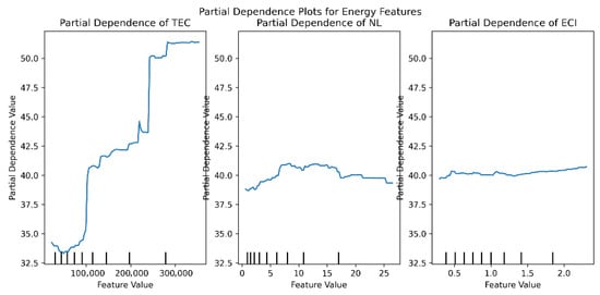
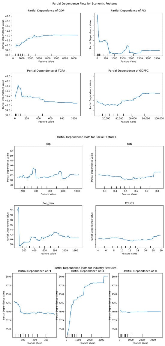
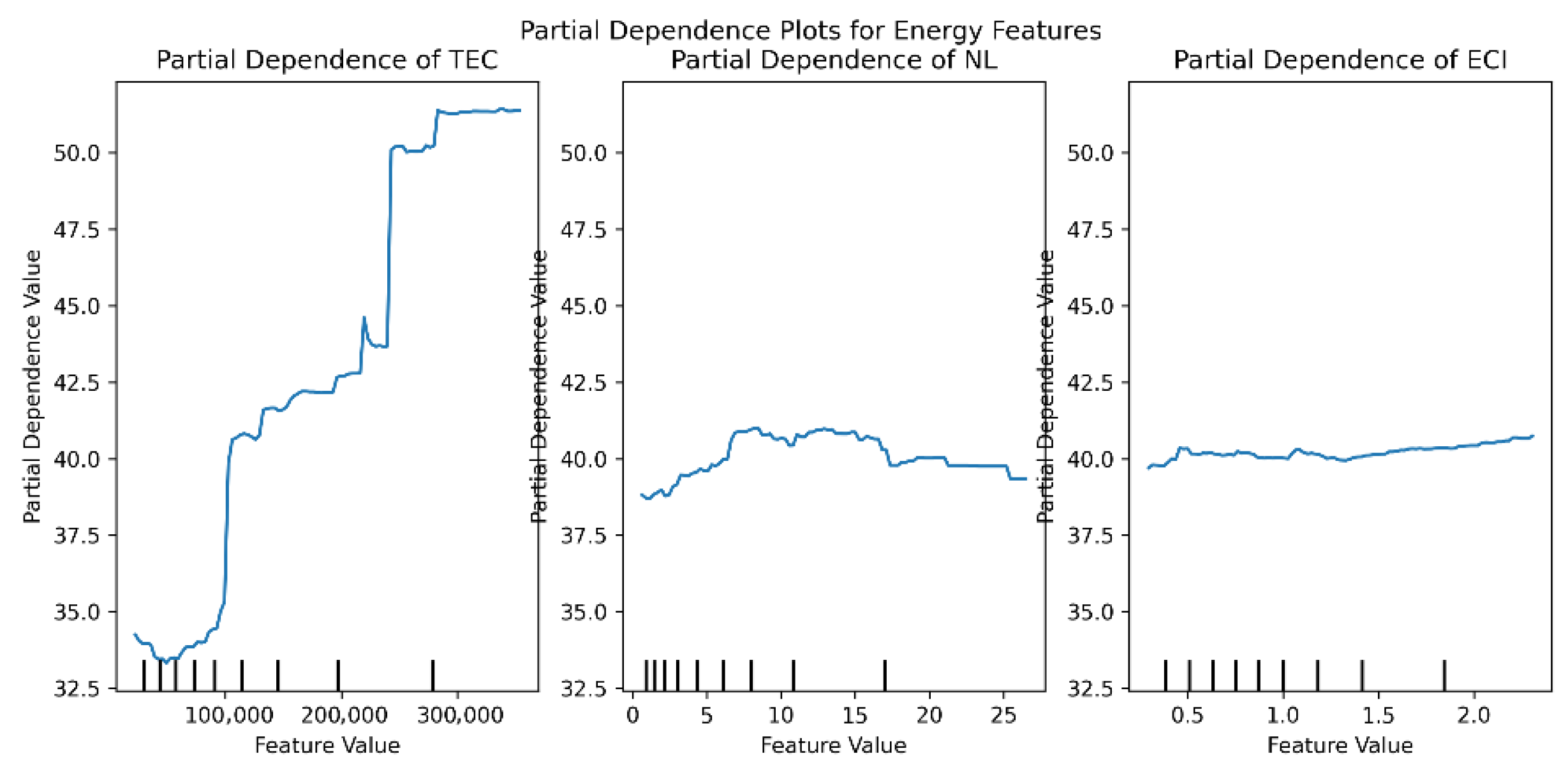
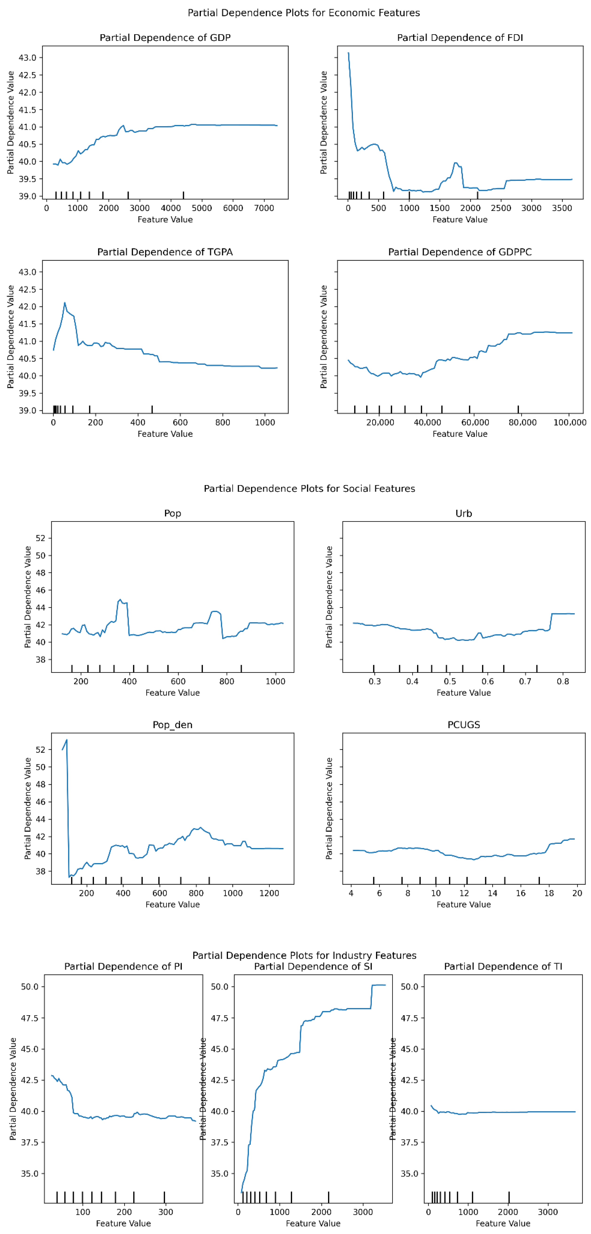
SHAP values provide detailed insights into individual predictions, revealing the specific contributions of each feature to the prediction of a particular instance. In contrast, PDPs offer a macro-level view of the overall impact of features on model predictions. Therefore, in this section, we conduct a visual analysis of different features based on Partial Dependence Plots (PDPs) as a complement to SHAP values. Figure 6 presents the partial dependence results for features from four different perspectives. By analyzing the Partial Dependence Plots (PDPs), this study can gain a deeper understanding of the relationship between the contributors of carbon reduction and pollution abatement and the model’s prediction results.

Figure 6. Partial Dependence plots.

In terms of economic characteristics, GDP growth exhibits a positive correlation with the intensity of carbon reduction and pollution abatement within a certain range. It can be observed that when the GDP eigenvalue is below 3000, its marginal effect on the prediction outcome continues to rise; after exceeding 3000, the marginal effect tends to stabilize—3000 can be regarded as the nonlinear turning point of GDP. This phenomenon aligns with the “diminishing marginal effect” logic of neoclassical growth theory: in the early stages of economic development, GDP expansion has a strong positive driving effect on the target variable; however, as the economic scale expands, diminishing marginal returns on capital weaken the marginal contribution of GDP. This is attributed to the fact that, in the early stages of development, rapid economic expansion is often propelled by high-pollution sectors such as manufacturing. The PDP of FDI exhibits a “sharp initial decline followed by fluctuating stabilization” pattern: when FDI is below 500, its marginal effect on predicted outcomes shows a significant negative decline; beyond 500, the marginal effect stabilizes—thus, 500 serves as the threshold point for FDI. This nonlinear relationship can be explained by the “FDI quality threshold” theory. It may initially exert a negative environmental impact due to the introduction of high-pollution projects, yet as investment deepens, its positive effects on carbon reduction and pollution abatement become more pronounced—likely owing to the advanced technologies and managerial practices introduced by foreign capital. The positive influence of TGPA (presumed to represent green patent quantity) at low values may stem from insufficient emphasis on green innovation during the early phases of economic development, when the intensity of carbon reduction and pollution abatement remains elevated. The stable trend of GDPPC (GDP per capita) indicates that per capita economic development has a limited direct impact on carbon reduction and pollution abatement efforts.

Regarding energy characteristics, the upward trajectory of TEC (Total Energy Consumption) directly reflects the promoting effect of increased energy use on carbon reduction and pollution abatement intensity. Meanwhile, the stable trend of ECI (Energy Consumption Intensity) suggests that optimizations in energy consumption structure may exert an indirect influence on these environmental outcomes.

In industrial dimensions, the trends of PI (Primary Industry share) and TI (Tertiary Industry share) indicate that both the primary and tertiary sectors contribute to enhancing carbon reduction and pollution abatement. Notably, SI (Secondary Industry share) displays a strong positive impact on abatement and reduction intensity, directly underscoring that the secondary industry remains the primary source of pressure for these efforts.

Socially, the positive impacts of Pop (Population Size) and Pop_den (Population Density) may be linked to scale and agglomeration effects arising from population concentration. Conversely, the fluctuating trend of Urb (Urbanization Rate) could reflect the varying environmental implications of urbanization across different developmental stages. The PDP of Urb shows that when the urbanization rate is in the range of 0.3–0.7, the partial dependence value of carbon emission intensity remains stable with a slight decline; it rises significantly after exceeding 0.7—0.7 is the nonlinear turning point of urbanization rate. This aligns with the Environmental Kuznets Curve (EKC) logic of urbanization: in the low urbanization stage (<0.7), population concentration in cities can reduce per-unit carbon emissions through “infrastructure sharing” (e.g., centralized heating); in the high urbanization stage (>0.7), consumption upgrading (e.g., private car ownership, expansion of high-energy-consuming service industries) becomes dominant, instead driving up carbon emission intensity.

These partial dependence plots elucidate the complex interrelationships between diverse features and pollution abatement/carbon reduction intensity, offering critical insights for optimizing strategic interventions in this domain.

5. Conclusions

To explore whether energy-related factors remain the primary barrier to carbon reduction and pollution abatement, this study, through a review of the literature and theories related to carbon reduction and pollution abatement, comprehensively selected four relevant domains: social, economic, industrial, and energy. From these domains, fourteen secondary indicators were chosen to characterize the contributors of carbon reduction and pollution abatement. Based on comparative analyses of multiple machine learning models, and through comparisons using various metrics, it was found that the XGBoost model performed the best. Using SHAP values and PDPs from explainable machine learning, the impacts of various contributors on carbon and pollution emissions was determined, providing suggestions for policymakers. The conclusions of this study are as follows:

(1)

Among the key driving factors, total energy consumption (TEC) exerts a dominant driving effect on urban carbon and pollutant emissions. The core logic lies in the fact that energy serves as a fundamental input supporting economic production and human social activities—whether it is industrial production, infrastructure operation, or residents’ daily living needs, all are highly dependent on energy consumption. Moreover, the large-scale utilization of energy (especially fossil energy) is directly linked to changes in the total emissions of carbon and pollutants. Meanwhile, the increase in the added value of the secondary industry (SI) and the expansion of population scale are also key factors driving the rise in emission intensity: the development of energy-intensive sectors such as heavy industry and manufacturing in the secondary industry directly drives the demand for energy consumption, thereby exacerbating emissions; in contrast, the growth of population scale indirectly drives up emission intensity by expanding residential energy consumption and increasing the demand for supporting infrastructure.

(2)

In terms of the model, the SHAP value analysis of explainable machine learning provides an in-depth understanding of model predictions, revealing which variables have the greatest impact on pollution and carbon emissions. By visualizing the internal workings of the model, a better analysis of the impact of various features on the target can be achieved. In this study, XGBoost achieved the best performance, with an R2 of 0.90, MSE of 83.3, MAE of 5.75, and MAPE of 0.15, demonstrating its good handling capability on non-linear datasets. Furthermore, the use of SHAP value algorithms and PDPs provides a comprehensive and balanced perspective to evaluate and interpret the behavior of the model. Through this integrated approach, we can more accurately identify and interpret the key contributors affecting model predictions, providing a solid foundation for decision-making.

(3)

Here, we present some specific examples of how the “energy barrier” could translate into specific policy levers. Firstly, for high-energy-consuming sub-sectors in the secondary industry such as steel, chemicals, and building materials, industry-specific energy efficiency benchmarks should be established and energy efficiency compliance should be linked with the promotion of green patent technologies. Secondly, a “Low-Carbon Transition Compensation Mechanism for Secondary Industries” should be established: For cities with a high proportion of secondary industries but weak economic foundations (such as resource-based cities in central and western regions), central fiscal transfers should be used to offset short-term economic losses during the “reduction of secondary industries” process, preventing the suppression of livelihood security due to emission reduction efforts.

(4)

Given China’s vast territory, there are significant differences in the development status of various cities and regions. Even within the same city, the development priorities and outcomes may vary greatly from year to year. Therefore, for different contributors, it is necessary to formulate localized policies tailored to the unique conditions of each city. Regional heterogeneity is an important consideration, with notable distinctions between coastal and inland areas, as well as between industry-dominated and service-dominated regions. For example, the service sector in coastal areas is generally more developed, while inland regions rely more on industry to drive growth. Additionally, the climatic conditions between coastal and inland areas differ significantly, which may further influence the effectiveness of policies such as energy transition.

References

- Yang, Y. Energy Globalization of China: Trade, Investment, and Embedded Energy Flows. J. Geogr. Sci. 2022, 32, 377–400. [Google Scholar] [CrossRef] [Scilit]
- IEA. World Energy Outlook 2024—Analysis. Available online: https://www.iea.org/reports/world-energy-outlook-2024 (accessed on 14 May 2025).
- Wolf, M.J.; Emerson, J.W.; Esty, D.C. Environmental Performance Index; Yale Center for Environmental Law & Policy: New Haven, CT, USA, 2022. [Google Scholar]
- Liu, Q.; Yang, Y.; Liu, Y.; Qian, X. Revealing Guangdong’s Bridging Role in Embodied Energy Flows Through International and Domestic Trade. Energies 2025, 18, 5607. [Google Scholar] [CrossRef] [Scilit]
- Guan, D.; Su, X.; Zhang, Q.; Peters, G.P.; Liu, Z.; Lei, Y.; He, K. The socioeconomic drivers of China’s primary PM2.5 emissions. Environ. Res. Lett. 2014, 9, 024010. [Google Scholar] [CrossRef] [Scilit]
- Meng, J.; Yang, H.; Yi, K.; Liu, J.; Guan, D.; Liu, Z.; Mi, Z.; Coffman, D.M.; Wang, X.; Zhong, Q.; et al. The slowdown in global air-pollutant emission growth and contributors. One Earth 2019, 1, 138–148. [Google Scholar] [CrossRef] [Scilit]
- Wei, Y.; Zhu, X.; Li, Y.; Yao, T.; Tao, Y. Influential contributors of national and regional CO2 emission in China based on combined model of DPSIR and PLS-SEM. J. Clean. Prod. 2019, 212, 698–712. [Google Scholar] [CrossRef] [Scilit]
- Ma, Q.; Tariq, M.; Mahmood, H.; Khan, Z. The nexus between digital economy and carbon dioxide emissions in China: The moderating role of investments in research and development. Technol. Soc. 2022, 68, 101910. [Google Scholar] [CrossRef] [Scilit]
- Huang, F.; Zhou, D.; Wang, Q. Decomposition and attribution analysis of the transport sector’s carbon dioxide intensity change in China. Transp. Res. Part A Policy Pract. 2019, 119, 343–358. [Google Scholar] [CrossRef] [Scilit]
- Ma, W.; Zhao, L.; Wang, N. Research on Contributors of Carbon reduction and pollution abatement in Yangtze River Delta Urban Agglomeration. J. Ecol. Rural Environ. 2022, 38, 1273–1281. [Google Scholar] [CrossRef]
- Li, Y.; Dai, J.; Zhao, H. Analysis of collaborative emission reduction of air pollutants and greenhouse gases under carbon neutrality target: A case study of Beijing, China. Clean Technol. Environ. Policy 2023, 26, 3995–4008. [Google Scholar] [CrossRef] [Scilit]
- Li, Y.; Chen, B.; Fang, D. Drivers of energy-related PM2.5 emissions in the Jing-Jin-Ji region between 2002 and 2015. Appl. Energy 2021, 288, 116668. [Google Scholar] [CrossRef] [Scilit]
- Han, D.; Diao, Y.; Wang, X. Spatial Network Correlation Characteristics and Contributors of the Synergistic Governance Efficiency of Carbon reduction and pollution abatement in the Yellow River Basin. Environ. Sci. 2025, 46, 3592–3603. [Google Scholar] [CrossRef] [Scilit]
- Yu, X.; Liang, Z.; Fan, J. Spatial decomposition of city-level CO2 emission changes in Beijing-Tianjin-Hebei. J. Clean. Prod. 2021, 296, 126613. [Google Scholar] [CrossRef] [Scilit]
- Huang, J.; Liu, C.; Chen, S. The convergence characteristics of China’s carbon intensity: Evidence from a dynamic spatial panel approach. Sci. Total Environ. 2019, 668, 685–695. [Google Scholar] [CrossRef] [Scilit] [PubMed]
- Lin, B.; Zhu, J. Energy and carbon intensity in China during the urbanization and industrialization process: A panel VAR approach. J. Clean. Prod. 2017, 168, 780–790. [Google Scholar] [CrossRef] [Scilit]
- Wang, S.; Zhu, X.; Song, D. Drivers of CO2 emissions from power generation in China based on modified structural decomposition analysis. J. Clean. Prod. 2019, 220, 1143–1155. [Google Scholar] [CrossRef] [Scilit]
- Wang, Q.; Chiu, Y.-H.; Chiu, C.-R. Driving factors behind carbon dioxide emissions in China: A modified production-theoretical decomposition analysis. Energy Econ. 2015, 51, 252–260. [Google Scholar] [CrossRef] [Scilit]
- Xu, B.; Lin, B. Regional differences in the CO2 emissions of China’s iron and steel industry: Regional heterogeneity. Energy Policy 2016, 88, 422–434. [Google Scholar] [CrossRef] [Scilit]
- Alimujiang, A.; Jiang, P. Synergy and co-benefits of reducing CO2 and air pollutant emissions by promoting electric vehicles—A case of Shanghai. Energy Sustain. Dev. 2020, 55, 181–189. [Google Scholar] [CrossRef] [Scilit]
- Yang, J.; Cai, W.; Ma, M. Driving forces of China’s CO2 emissions from energy consumption based on Kaya-LMDI methods. Sci. Total Environ. 2020, 711, 134569. [Google Scholar] [CrossRef] [Scilit]
- Zhang, J.; Zeng, W.; Wang, J. Regional low-carbon economy efficiency in China: Analysis based on the Super-SBM model with CO2 emissions. J. Clean. Prod. 2017, 163, 202–211. [Google Scholar] [CrossRef] [Scilit]
- Han, Y.; Long, C.; Geng, Z. Carbon emission analysis and evaluation of industrial departments in China: An improved environmental DEA cross model based on information entropy. J. Environ. Manag. 2018, 205, 298–307. [Google Scholar] [CrossRef] [Scilit] [PubMed]
- Zhang, S.; Zhao, T. Identifying major influencing contributors of CO2 emissions in China: Regional disparities analysis based on STIRPAT model from 1996 to 2015. Atmos. Environ. 2019, 207, 136–147. [Google Scholar] [CrossRef] [Scilit]
- Yang, S.; Cao, D.; Lo, K. Analyzing and optimizing the impact of economic restructuring on Shanghai’s carbon emissions using STIRPAT and NSGA-II. Sustain. Cities Soc. 2018, 40, 44–53. [Google Scholar] [CrossRef] [Scilit]
- Cong, X.; Zhao, M.; Li, L. Analysis of carbon dioxide emissions of buildings in different regions of China based on STIRPAT model. Procedia Eng. 2015, 121, 645–652. [Google Scholar] [CrossRef] [Scilit]
- Zhong, S.; Zhang, K.; Bagheri, M. Machine learning: New ideas and tools in environmental science and engineering. Environ. Sci. Technol. 2021, 55, 12741–12754. [Google Scholar] [CrossRef] [Scilit]
- Brokamp, C.; Jandarov, R.; Rao, M.B.; LeMasters, G.; Ryan, P. Exposure assessment models for elemental components of particulate matter in an urban environment: A comparison of regression and random forest approaches. Atmos. Environ. 2017, 151, 1–11. [Google Scholar] [CrossRef] [Scilit]
- Hu, X.; Belle, J.H.; Meng, X.; Wildani, A.; Waller, L.A.; Strickland, M.J.; Liu, Y. Estimating PM2.5 concentrations in the conterminous United States using the random forest approach. Environ. Sci. Technol. 2017, 51, 6936–6944. [Google Scholar] [CrossRef] [Scilit]
- Wen, Y.; Wu, R.; Zhou, Z. A data-driven method of traffic emissions mapping with land use random forest models. Appl. Energy 2022, 305, 117916. [Google Scholar] [CrossRef] [Scilit]
- Yu, W.; Xia, L.; Cao, Q. A machine learning algorithm to explore the drivers of carbon emissions in Chinese cities. Sci. Rep. 2024, 14, 23609. [Google Scholar] [CrossRef] [Scilit]
- Kumari, S.; Singh, S.K. Machine learning-based time series models for effective CO2 emission prediction in India. Environ. Sci. Pollut. Res. 2023, 30, 116601–116616. [Google Scholar] [CrossRef] [Scilit]
- Zuo, Z.; Guo, H.; Cheng, J. An LSTM-STRIPAT model analysis of China’s 2030 CO2 emissions peak. Carbon Manag. 2020, 11, 577–592. [Google Scholar] [CrossRef] [Scilit]
- Liu, F.; Wang, R.; Fang, M. Mapping green innovation with machine learning: Evidence from China. Technol. Forecast. Soc. Change 2024, 200, 123107. [Google Scholar] [CrossRef] [Scilit]
- Ma, L.; Graham, D.J.; Stettler, M.E.J. Using explainable machine learning to interpret the effects of policies on air pollution: COVID-19 lockdown in London. Environ. Sci. Technol. 2023, 57, 18271–18281. [Google Scholar] [CrossRef] [Scilit] [PubMed]
- Chen, T.; Guestrin, C. Xgboost: A scalable tree boosting system. In Proceedings of the 22nd ACM SIGKDD International Conference on Knowledge Discovery and Data Mining, San Francisco, CA, USA, 13–17 August 2016; pp. 785–794. [Google Scholar] [CrossRef] [Scilit]
- Yang, C.; Liu, L.L.; Huang, F.M.; Huang, L.; Wang, X.M. Machine learning-based landslide susceptibility assessment with optimized ratio of landslide to non-landslide samples. Gondwana Res. 2023, 123, 198–216. [Google Scholar] [CrossRef] [Scilit]
- Zheng, J.; Wang, P.; Shi, H.; Zhuang, C.; Deng, Y.; Yang, X.; Huang, F.; Xiao, R. Quantitative source apportionment and driver identification of soil heavy metals using advanced machine learning techniques. Sci. Total Environ. 2023, 873, 162371. [Google Scholar] [CrossRef] [Scilit]
- Dai, L.; Ge, J.; Wang, L.; Zhang, Q.; Liang, T.; Bolan, N.; Lischeid, G.; Rinklebe, J. Influence of soil properties, topography, and land cover on soil organic carbon and total nitrogen concentration: A case study in Qinghai-Tibet plateau based on random forest regression and structural equation modeling. Sci. Total Environ. 2022, 821, 153440. [Google Scholar] [CrossRef] [Scilit]
- Oukawa, G.Y.; Krecl, P.; Targino, A.C. Fine-scale modeling of the urban heat island: A comparison of multiple linear regression and random forest approaches. Sci. Total Environ. 2022, 815, 152836. [Google Scholar] [CrossRef] [Scilit]
- Ke, G.; Meng, Q.; Finley, T.; Wang, T.; Chen, W.; Ma, W. Lightgbm: A highly efficient gradient boosting decision tree. Adv. Neural Inf. Process. Syst. 2017, 30, 3149–3157. [Google Scholar]
- Schapire, R.E. Explaining adaboost. In Empirical Inference: Festschrift in Honor of Vladimir N. Vapnik; Springer: Berlin/Heidelberg, Germany, 2013; pp. 37–52. [Google Scholar] [CrossRef] [Scilit]
- Ranstam, J.; Cook, A. LASSO regression. J. Br. Surg. 2018, 105, 1348. [Google Scholar] [CrossRef] [Scilit]
- Lundberg, S. A unified approach to interpreting model predictions. arXiv 2017, arXiv:1705.07874. [Google Scholar] [CrossRef] [Scilit]
- Moosbauer, J.; Herbinger, J.; Casalicchio, G. Towards explaining hyperparameter optimization via partial dependence plots. In Proceedings of the 8th ICML Workshop on Automated Machine Learning (AutoML), Online, 23–24 July 2021. [Google Scholar]
Disclaimer/Publisher’s Note: The statements, opinions and data contained in all publications are solely those of the individual author(s) and contributor(s) and not of MDPI and/or the editor(s). MDPI and/or the editor(s) disclaim responsibility for any injury to people or property resulting from any ideas, methods, instructions or products referred to in the content. |
© 2026 by the authors. Licensee MDPI, Basel, Switzerland. This article is an open access article distributed under the terms and conditions of the Creative Commons Attribution (CC BY) license.