Analysis of Influence of Nanoparticle Properties on Nanofluid Thermomagnetic Convection Through Modification of System of Forces

Abstract

The tendency to design compact systems results in limited space for particular components and heat transfer processes, which influences the removal of heat. Therefore, new methods for heat transfer intensification are being designed. Coupling passive and active methods of heat transfer intensification seems to be a promising approach toward removing high-heat-rate values from a system. The main purpose of the investigation presented was numerical analysis of the influence of nanoparticle materials on the heat transfer processes occurring during thermal convection in the Rayleigh–Benard system configuration under a strong magnetic field environment. The combination of the usage of nanoparticles and a strong magnetic field as one of the options will be justified for its suitability in heat transfer processes. Two types of nanofluids were analysed, namely water-silver and water-copper oxide, with a 0.25 [vol.%] particle concentration, in both cases. The numerical approach considered the nanofluid as the two-phase fluid and was realised in Comsol Multiphysics. Due to the magnetic field, new forces appeared in the system. These forces depend on the magnetic field orientations, and in one orientation, they caused the transfer of higher heat rates by copper oxide nanofluid by 15 [%], while the second one saw the attenuation of natural convection. Silver nanoparticles, because of their weaker magnetic character, intensified heat transfer by approximately 10 [%]. Therefore, copper oxide seems to be a better option for industrial applications.

1. Introduction

Nanofluids have continuously attracted interest since their first appearance. Understanding their properties and the development of production technologies increases the search for new areas of application [1]. They can be applied in a wide variety of fields, such as energy engineering, medicine, or the cosmetics industry. Energy engineering, which is within the authors’ scope of interest, is expanding by itself, and at this moment, nanofluids are considered as potential fluids in fields, such as machining, cooling systems, energy storage [2] and heat exchangers [3].

Research considering other modifications of the composition of nanofluids and investigation methods is also being developed, taking into account the growing popularity of hybrid nanofluids (containing two or more types of nanoparticles or base fluids) [4] or analytical and experimental research methods extended by numerical methods and including artificial intelligence algorithms [5]. All presented publications pointed out the significance of nanofluid properties and their influence on the processes occurring in systems; however, they did not discuss in detail the mechanisms of interaction between the fluid and the particles and between the particles.

Another method that could enhance heat transfer is the use of an external energy source, such as a magnetic field. There are a number of studies on the effect of a strong magnetic field on weakly magnetic fluids. Research on the forced flow in a pipe (diameter 0.04 [m]) of weakly magnetic fluid, which was air, with both low [6] and larger [7] Reynolds number values (16, 547, 1369 and 2190), was presented. The temperature difference was 5, 40 and 70 [K], and magnetic induction was in the range of 1–10 [T]. The numerical results indicated that the direction of flow can be modified by introducing an additional magnetic force into the system. Experimental and numerical studies on paramagnetic fluid in an enclosure using a strong magnetic field were also conducted [8]. The laminar−turbulent transition during thermomagnetic convection for the thermomagnetic Rayleigh number (Ra_TM) order of magnitude 10⁷ was studied using thermal plumes.

The possibility of increasing heat transfer processes and changing the flow structure with the help of magnetic fields was proven. The papers mentioned provided insights into the interaction between fluid and magnetic and gravity fields.

A comprehensive review of the natural convection of nanofluids in square enclosures was shown in [9]. Most of the studies cited were based on numerical simulations, and only a few were experimental in nature. It was observed that the presence of a magnetic field reduced heat transfer, except in a few cases, where it was enhanced at certain values. The examined Hartmann number ranged from 0 to 60 and even to 100. The Rayleigh number values were in the range of 10⁴–10⁶. The non-magnetic particles most frequently mentioned were Al₂O₃, CuO, CNT, Cu, and TiO₂. In some of the cases discussed, attention was drawn to forces that act on the flow characteristics or heat transfer processes. However, this was mainly the Lorentz force.

Research on the convective heat transfer of water-based nanofluids with copper oxide nanoparticles within an isosceles triangular geometry with an uneven bottom wall should be mentioned [10]. The non-homogeneous dynamic model represents convective nanofluid flow, and the finite element method was used to solve the system of equations with boundary conditions. The results of the study indicate an increase in heat transfer through the use of nanoparticles and a reduction in their diameter. However, significant reductions in fluid flow, heat transfer processes, and nanoparticle concentration were also observed as the strength of the magnetic field effect increased. The broad analysis did not focus on detailed studies of how the behaviour of the nanofluid components was influenced by the magnetic field.

Despite these developments, there remains a significant research gap concerning the fundamental mechanism of weakly magnetic nanofluids under strong magnetic fields. Most of the existing literature focusses on materials with strong magnetic properties, neglecting substances that, although common in the environment, have weak magnetic properties. This study fills this gap by applying a two-phase flow model that takes into account interactions between the magnetic field and individual components of the nanofluids studied. The combination of different magnetic properties of the base fluid (water—diamagnetic) and nanoparticles (Ag—diamagnetic, CuO—paramagnetic) makes it possible to analyse a complex phenomenon.

This work focusses mainly on the numerical analysis of the effect of the type of nanoparticles on the phenomena present in environments with different strong magnetic field orientations in the system, consisting of a cube with differentially heated top and bottom walls. Attention is paid to the heat transfer and origins of changes in the flow structure as a result of the existence of the gravity and magnetic forces acting both on the fluid and nanoparticles. The novelty comes from evaluation of the influence of magnetic force on the processes analysed, which was quantified separately for base fluid and nanoparticles. To the knowledge of the authors, this approach has been reported in the literature, together with a comparison with the experiment, only by our research group [11].

2. Numerical Model

The computational domain was a cubic system with thermally active horizontal walls and adiabatic side walls placed under the influence of a strong magnetic field. Thermal convection was achieved by a temperature difference of 8 [K] between the horizontal walls, where the bottom wall was heated (at a temperature equal to 299 [K]) and the top wall was cooled (at a temperature equal to 291 [K]) as in the Rayleigh−Benard configuration.

The influence of the magnetic environment on the convection phenomenon studied was through the different orientations of the magnetic field and the different magnetic properties of the nanofluid components and their interaction.

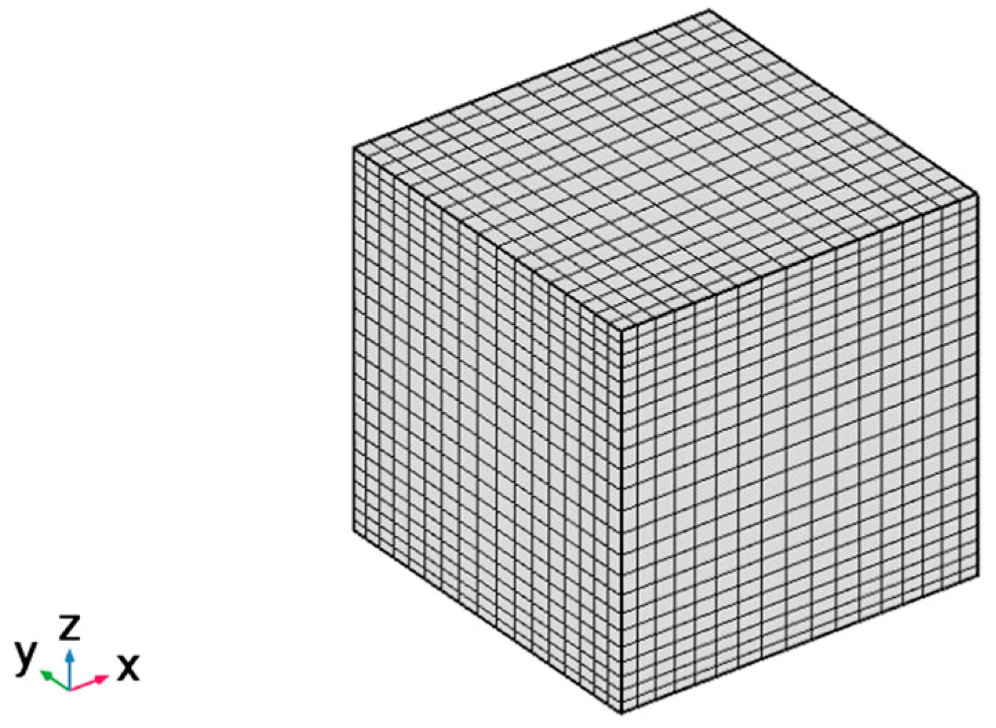
The numerical model was constructed in Comsol Multiphysics. The computational domain shown in Figure 1 was divided into 25 × 25 × 35 quadrilateral elements in the x, y, and z directions, respectively. It should be mentioned that the size of the cube was 32 × 10⁻³ [m]. The mesh was refined in the vicinity of the wall to properly represent the boundary layer. The first node was located at 5 × 10⁻⁵ [m] from the wall. The mesh met the requirements of the independence of the solution. The variable time step was applied with an upper limit set to 0.5 [s] to be equal to the frequency of the available data acquisition system. The convergence criterion for mass, momentum, and energy was set at the level of 10⁻⁶. The quality measures of the grids with various analysed elements are presented in

Table 1. Quality measures of the thermomagnetic convection model grids.

Number of Grid Elements	45,625	15,215	6864	Experiment
skewness	0.8829	0.8335	0.8090	−
volume versus length	0.4653	0.4333	0.4328	−
growth rate	0.5669	0.4383	0.3836	−
average value of the number Nu	12.357	12.235	11.618	12.23 ± 0.62

, while the selected grid is presented in Figure 1.

The initial conditions were set as follows: zero velocity and pressure distribution for the carrier and dispersed phases; the initial temperature inside the domain was the arithmetic mean of the heated and cooled horizontal walls. The boundary conditions were set as follows: the side walls were adiabatic, while the horizontal walls were at constant temperature (the temperature of the cooled wall was 291 [K], and the heated wall was tuned to the set temperature difference) and zero velocity on all walls of the computational domain.

2.1. Mass, Momentum and Energy Equations

The Euler−Euler two-phase model of nanofluid was considered. The mass and momentum balance equations for each phase [12] were defined:

• The mass balance for the carrier and dispersed phases was formulated as follows:

$$\nabla ·\left(\right(1-f){\rho }_c\mathbf{u}+f{\rho }_d\mathbf{v})=0$$

(1)

$$\nabla ·\left(f{\rho }_d\mathbf{v}\right)=0$$

(2)

• The momentum balance for the carrier and dispersed phases was formulated as follows:

$${\rho }_c{\displaystyle \frac{\mathsf{\partial }\mathbf{u}}{\partial t}}+{\rho }_c\left(\mathbf{u}·\nabla \right)\mathbf{u}=-\nabla ·\left(p\mathbf{I}\right)+\nabla ·{\mathsf{\tau }}_c+{\mathbf{F}}_{g,c}+{\mathbf{F}}_{m,c}+{\mathbf{F}}_{d,c}/\left(1-f\right)$$

(3)

$${\rho }_d{\displaystyle \frac{\partial \mathbf{v}}{\partial t}}+{\rho }_d\left(\mathbf{v}·\nabla \right)\mathbf{v}=-\nabla ·\left(p\mathbf{I}\right)+\nabla ·{\mathsf{\tau }}_d+{\mathbf{F}}_{g,d}+{\mathbf{F}}_{m,d}+{\mathbf{F}}_{d,d}/f$$

(4)

Body forces were defined as follows:

$${\mathbf{F}}_{g,c}={\rho }_{c,0}·{\beta }_{c,0}·\left(T-T_0\right)\mathbf{g}$$

(5)

$${\mathbf{F}}_{g,d}=\left[{\rho }_{c,0}·{\beta }_{c,0}·\left(T-T_0\right)-{\rho }_d\right]\mathbf{g}·f$$

(6)

$${\mathbf{F}}_{m,c}=-{\displaystyle \frac{{\chi }_{m,c}·{\rho }_{c,0}·{\beta }_{c,0}·\left(T-T_0\right)}{2{\mu }_0}}\nabla {\mathbf{B}}^2$$

(7)

$${\mathbf{F}}_{m,d}=-{\displaystyle \frac{{{\chi }_{m,d}·{\rho }_d-\chi }_{m,c}·{\rho }_{c,0}·{\beta }_{c,0}·\left(T-T_0\right)}{2{\mu }_0}}\nabla {\mathbf{B}}^2·f$$

(8)

$${\mathbf{F}}_{d,c}=-{\mathbf{F}}_{d,d}=\epsilon \left(\mathbf{v}-\mathbf{u}\right)$$

(9)

where t is time [s]; p is pressure [Pa]; f is the volume fraction of the dispersed phase [−]; u, v are the vectors of the carrier and dispersed phases velocity [m/s]; τ is the viscous stress tensors of the particular phase, [N/m²]; ρ is the density of particular phase density [kg/m³]; g is the gravitational acceleration [m/s²]; β is the thermal expansion coefficient of the particular phase [1/K]; T is the temperature [K]; T₀ is the reference temperature, equal to the average value of the temperature of the hot and cold walls [K]; χ_m is mass magnetic susceptibility (χ_m = χ/ρ) [m³/kg]; μ₀ is the magnetic permeability of the vacuum, 4π × 10⁻⁷, [H/m] = [N/A²]; $\nabla {\mathbf{B}}^2$ is the gradient of magnetic induction square [T²/m]; F_g and F_m are the volumetric forces (gravitational and magnetic vectors [N/m³]); index c represents a carrier phase (fluid), while index d is dispersed phase (the nanoparticles); and the symbol “0” indicates that the property represents the state at the reference temperature when there is no carrier phase (fluid) movement.

Equation (9) describes the interphase volumetric force, where F_d is the interphase body force [N/m³], and ε is the friction coefficient between the coexisting phases [kg/(m³s)].

Taking into account the domination of the base fluid, the thermal equilibrium between the nanofluid components was assumed.

The energy balance was modelled with the use of a single-phase model. In this case, for the thermal properties introduced in Equation (10), the weighted average values represent the carrier phase and the dispersed phase refers to the density (ρ), specific heat (c_p) and thermal conductivity (k):

$$\rho {\displaystyle \frac{\partial T}{\partial t}}+\rho ·c_p\left(\mathbf{u}·\nabla T\right)=\nabla ·\left(k\nabla T\right)$$

(10)

2.2. Magnetic Field Representation

The steady magnetic field can be described by the Maxwell equations:

$$\nabla \times \mathbf{H}=\mathbf{J}$$

(11)

$$\mathbf{B}=\nabla \times \mathbf{A}$$

(12)

where H is the magnetic field strength vector [A/m], B is the magnetic induction vector, $\mathbf{B}={\mu }_m\mathbf{H}$ [T], J is an electric current density vector, A is a magnetic field potential vector [Wb/m], μ_m is the magnetic permeability of the medium [H/m].

Equations (11) and (12) can be reduced to Amper’s law:

$$\nabla \times \left({{\mu }_m}^{-1}\nabla \times \mathbf{A}\right)=\mathbf{J}$$

(13)

It can be solved when the electrical current density is known.

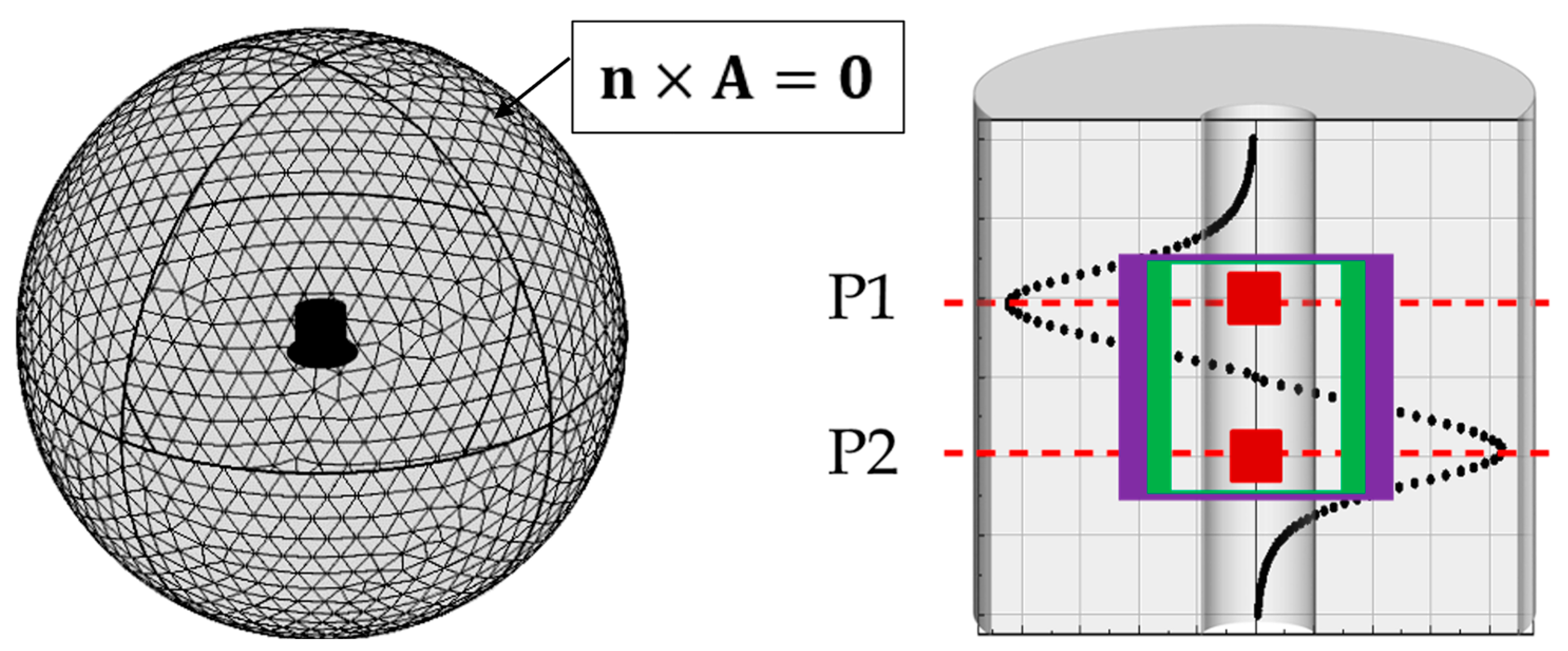
The calculation space considered consists of a shell of 4 [m] diameter, which covers the electrical solenoid (Figure 2). The boundary condition was represented by the decay of the magnetic field.

To calculate the vector of potential A, the finite element method was used, and then the magnetic induction distribution could be calculated.

In the reference cases without magnetic field influence, no induction or magnetic force was added to the system (magnetic induction B was equal to 0). Analysis of the influence of magnetic conditions was performed by applying the square of the magnetic induction at half of the height of the enclosure. In the first variant, called Position 1 (P1), the magnetic induction square was −680 [T²/m], and in the second variant (named P2), 680 [T²/m], which corresponded to 9 [T] of magnetic induction. A magnetic field decay sphere was implemented around the magnet, as presented in Figure 2 (left side), together with the boundary condition.

The magnetic field model was prepared in the multi-turn coil Comsol software module, which enabled the generation of a magnetic field based on the geometry details provided. The documentation of the real magnet, on the basis of which the presented model was prepared, did not define all the needed geometric parameters. The dimensions of two coils approximated by cylinders were given (the inner and outer diameters of the first coil were 0.13 [m] and 0.1984 [m], respectively (marked with a green rectangle), and the second coil’s were 0.208 [m] and 0.2814 [m], respectively (marked with a purple rectangle); the height of the coils was 0.2193 [m]). The remaining parameters, such as electrical current, number of turns, and wire dimensions, were arbitrarily selected so that the condition of 10 [T] magnetic induction was met in the centre of the magnet, and its distribution was consistent with the documentation provided. The diameter of the modelled wire was 0.001 [m], the cross−sectional area was 1 × 10⁻⁶ [m²], and the number of turns was 500. The other known geometric parameters were consistent with the magnet documentation.

The computational domain was located at the position corresponding to the maximum value of the square of the magnetic induction gradient (see Figure 2, right side).

The influences of the magnetic conditions on the convective phenomena were related to the computational domain position P1 or P2 and the magnetic properties of the substances.

2.3. Analysed Fluids

Water (as a reference case) and two types of nanofluids, which were typified by different solid particle materials, were used as working fluids in the phenomena studied. In both cases, the carrier phase was water, and the dispersed phase was a solid phase of 50 [nm]. In one case, it was in the form of silver nanoparticles (Ag), and in the other case, copper oxide (CuO) nanoparticles. The concentration of nanoparticles in both cases was 0.25 [vol.%], so the fluid names Ag0.25 and CuO_0.25 were used.

The properties of the selected substances play a key role in terms of the efficiency of heat transfer processes. The thermal properties of solid materials contribute to the thermal properties of the global fluid. The numerical values of the properties considered for the nanofluid components and their average values are listed in

Table 2. Properties of the working fluids.

Property at 20 °C	Water	Silver	Copper Oxide	Ag0.25	CuO_0.25
density [kg/m3]	998	10,500	6500	1022	1012
thermal expansion coefficient [1/K]	18.50 · 10−5	−	−	20.54 · 10−5	20.53 · 10−5
specific heat [J/(kg·K)]	4183	235	540	4172	4173
dynamic viscosity [kg/(m·s)]	10.60 · 10−4	−	−	10.11 · 10−4	10.10 · 10−4
thermal conductivity [W/(m·K)]	0.598	429	18	0.603	0.602
magnetic susceptibility [−]	−8.80 · 10−6	−2.38 · 10−5	2.44 · 10−4	−8.92 · 10−6	−7.03 · 10−6

.

Magnetic susceptibility describes the ability of a substance to be magnetised in the magnetic field. The paramagnetics are attracted toward the maximal value of magnetic induction, while the diamagnetics are repelled, and, therefore, the opposite effects of a magnetic field can be expected for them. The water is diamagnetic, as is the silver, while the copper oxide is paramagnetic.

3. Data Reduction

Simulations were performed for at least 1500 [s]. All further results were calculated as average values over 600 [s]. A widely used metric for the efficiency of convective heat transfer is the Nusselt number, which was calculated as the ratio of the average value of top or bottom horizontal walls’ heat rate (Q_{conv_ave} [W]) and the heat rate during the conduction process (Q_cond [W]). It can be written as follows:

$$\overline{\mathrm{N}\mathrm{u}}={\displaystyle \frac{Q_{conv\_ave}}{Q_{cond}}}={\displaystyle \frac{\frac{1}{2}\left[{\int }_{S_{\mathrm{c}\mathrm{o}\mathrm{l}\mathrm{d}}}{\left.\mathbf{q}·\mathbf{n}\right|}_{\mathrm{c}\mathrm{o}\mathrm{n}\mathrm{v},\mathrm{c}\mathrm{o}\mathrm{l}\mathrm{d}}d{S}_{\mathrm{c}\mathrm{o}\mathrm{l}\mathrm{d}}+{\int }_{S_{\mathrm{h}\mathrm{o}\mathrm{t}}}{\left.\mathbf{q}·\mathbf{n}\right|}_{\mathrm{c}\mathrm{o}\mathrm{n}\mathrm{v},\mathrm{h}\mathrm{o}\mathrm{t}}d{S}_{\mathrm{h}\mathrm{o}\mathrm{t}}\right]}{Q_{cond}}}$$

(14)

where n is the normal vector to the surface [−]; q is the heat flux density, [W/m²]; S_cold and S_hot are the cooled and heated wall areas, respectively, [m²] (both equal to 0.001024 [m²]).

The heat flux perpendicular to the heated and cooled surfaces was calculated on the basis of the temperature distribution obtained at each time point. The conducted heat flux was determined using Fourier’s law.

To investigate the contribution of the magnetic field, the results related to heat transfer processes were presented as the ratio of the Nusselt number (Nu) to its value obtained without the magnetic field influence (Nu_0T).

To describe the combined effect of thermal and magnetic conditions, the thermomagnetic Rayleigh number (Ra_TM) was introduced and defined as follows:

$${\mathrm{R}\mathrm{a}}_{\mathrm{T}\mathrm{M}}={\mathrm{R}\mathrm{a}}_{\mathrm{T}}\left[1-{\displaystyle \frac{{\chi }_m}{{\mu }_{0}g}}{B}_z{\displaystyle \frac{\partial B_z}{\partial z}}\right]$$

(15)

where Ra_T indicates the thermal Rayleigh number represented by the following equation:

$${\mathrm{R}\mathrm{a}}_{\mathrm{T}}={\displaystyle \frac{g\beta {\varrho }^2{c}_p}{\mu k}}{d}^3\mathsf{\Delta }T$$

(16)

g is the magnitude of gravitational acceleration [m/s²]; β is the thermal expansion coefficient [1/K]; ρ is the density [kg/m³]; c_p is the specific heat [J/(kg·K)]; μ is the dynamic viscosity [kg/(m·s)]; k is the thermal conductivity [W/(m·K)]; d is the characteristic dimension [m]; ΔT is the temperature difference [K]; χ_m is the mass magnetic susceptibility [m³/kg]; B_z is the magnitude axial component of the magnetic induction vector B [T]; μ₀ is the magnetic permeability of vacuum [H/m].

The value of the Ra_TM number depends on the thermal and magnetic conditions. At position P1 of the computational domain in the magnetic field, the magnetic component in Equation (15) takes a negative value. The higher the value of magnetic induction at P1, the more negative the magnetic part becomes, and, therefore, Ra_TM is lower than Ra_T. Similarly, in position P2 of the computational domain in the magnetic field, the values of the magnetic component are positive and increase with increasing magnetic induction values.

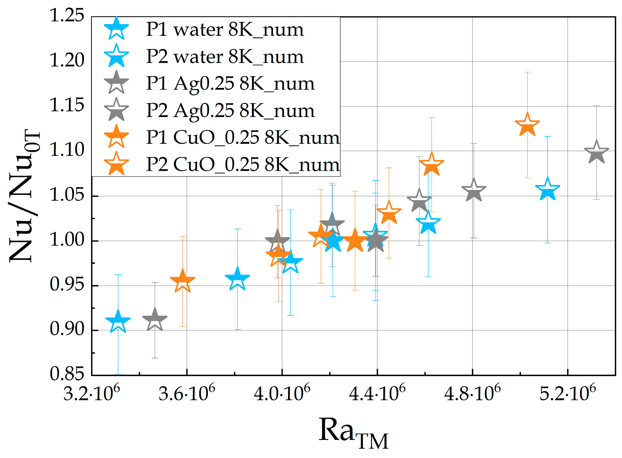
Figure 3 shows the results of the Nusselt number ratio versus the thermomagnetic Rayleigh number (Ra_TM) for water, Ag0.25 and CuO_0.25 nanofluids. The averaged Nusselt numbers were referenced each time to the value without a magnetic field. The uncertainty of the average Nusselt number was the standard deviation, while for the Nusselt number ratio, the uncertainty was determined using the law of propagation of uncertainty and added to Figure 3.

The thermomagnetic Rayleigh number (Ra_TM) values cover a wide range, as both positions P1 and P2 in the magnetic field are considered. The results are represented by the star symbol, water in blue, for nanofluids with silver in grey, and copper oxide in orange. Symbols filled with colour only in the upper half show results for position P1, while those filled in the lower half show results for position P2. Fully filled symbols are obtained without the influence of a magnetic field (0 [T] case).

It can be seen that the results of numerical analysis exhibit a clear trend: at position P1, the values of the Nu/Nu_0T ratio for each fluid decrease with increasing magnetic induction and are lower than 1. However, at position P2, they increase and take higher values than 1. The magnetic part causes a decrease in Ra_T at position P1 and an increase at position P2. The relationship appears to be close to linear, with the Nu/Nu_0T values being the lowest for water and the highest for the copper oxide nanofluid.

These results could be explained only through (1) the magnetic properties and (2) the effect of the magnetic field (direction of action) on the individual components of the nanofluids, in each position, because of the introduction into the system of new forces.

Understanding of System of Forces

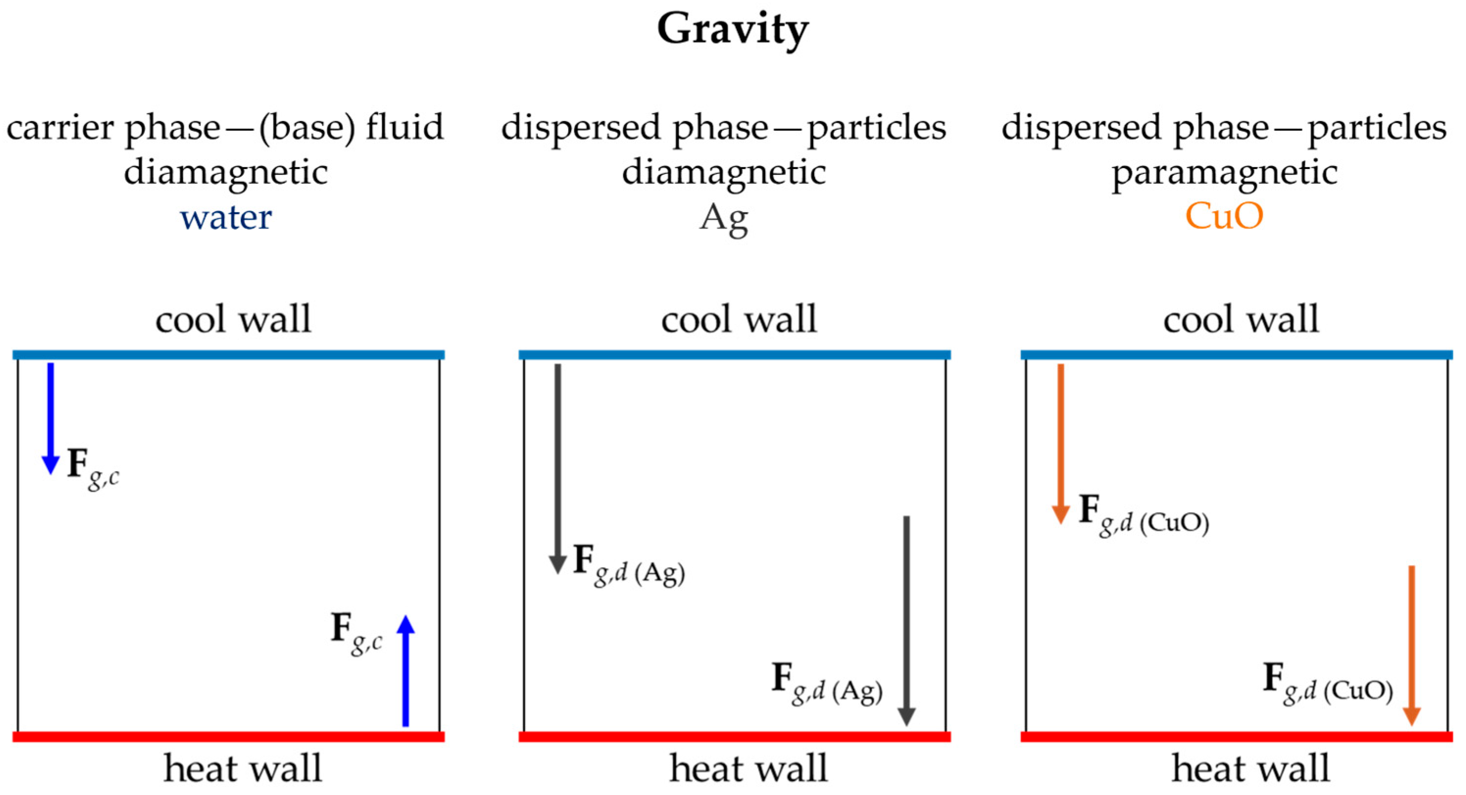
The gravitational buoyancy force that occurs during thermal convection, acting on water (diamagnetic fluid), silver (diamagnetic nanoparticles), and copper oxide (paramagnetic nanoparticles), is schematically presented in Figure 4.

The first column on the left represents the orientation and direction of the gravitational buoyancy force acting on the water. It can be said that the temperature difference causes a difference in fluid density near the heated and cooled walls, which is why the warmer fluid lifts upward, while the colder fluid falls downward. Therefore, the unit force of gravitational buoyancy depends on the set temperature difference but also on the properties of the substance under investigation. The middle column shows the orientation and direction of the unit gravitational force acting on Ag nanoparticles, marked in grey. This force is directed downward, both near the heated and the cooled walls. In the third column (on the right), the unit gravitational force acting on CuO nanoparticles is represented by orange. This force is also directed downwards.

From the point of view of the value of gravitational force, the most important factors are physical properties, in particular the density of the substance under investigation. Therefore, the gravitational force acting on Ag nanoparticles is greater than the force acting on CuO nanoparticles (as shown in the diagram (in Figure 4) by the length of the arrows symbolising the force).

When considering the magnetic buoyancy force, it is necessary to distinguish which position is being analysed. In positions P1 and P2, the orientation and value of the force will depend on the properties of the substance being analysed (including its magnetic properties). CuO particles have the highest absolute magnetic susceptibility value (it is an order of magnitude higher than that of the diamagnetic substances mentioned here). The second key factor that influences the direction and value of this force is the magnetic field parameter, i.e., gradB_z², which takes negative values in position P1 and positive values in position P2.

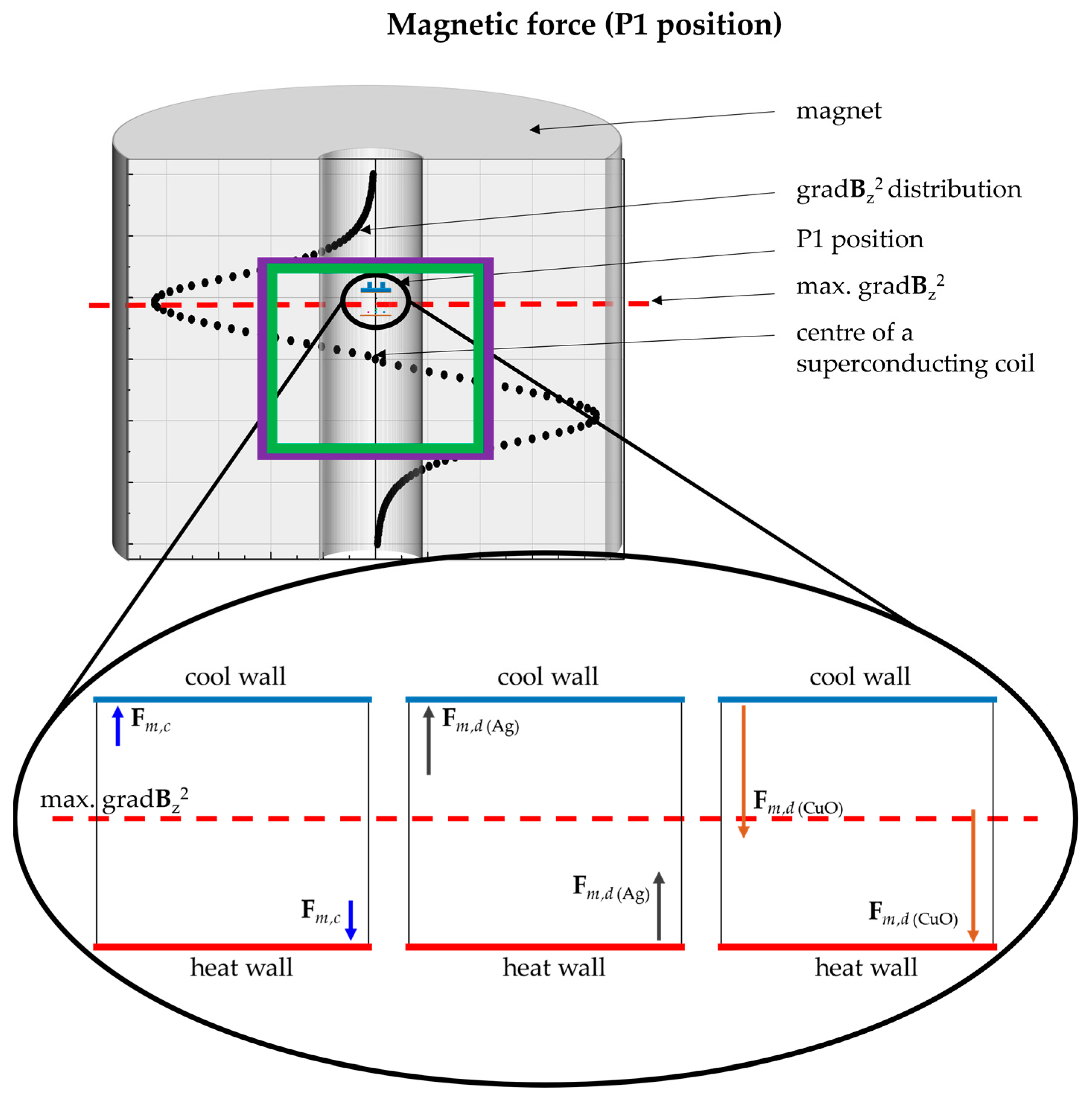
Figure 5 shows the unit magnetic buoyancy force acting on water (left side), Ag nanoparticles (centre), and CuO nanoparticles (right side) at position P1.

In general, diamagnetic substances are repelled from a strong magnetic field, which in Figure 5 is represented by the centre of the coil and the highest value of magnetic induction. In the case of a diamagnetic fluid, taking into account the definition of unit magnetic buoyancy force (Equation (7)), an important parameter that changes the direction of the acting force is the temperature difference. The action of the force near the upper, cooled wall has a positive sign and is directed upward. Then, near the bottom wall, it is directed downwards.

The Ag nanoparticles, which are also diamagnetic, are repelled by a magnetic field. The influence of the medium in which they are located has been taken into account in the formulation of the magnetic buoyancy force acting on the nanoparticles (Equation (8)). However, it should be noted that this influence is marginally small (of the order of 10⁻⁹). Therefore, the factors that actually determine the value and direction of the force are the properties of the particles (density, magnetic susceptibility) and the magnetic field parameter (gradB_z²). In the case of Ag nanoparticles in P1, the force acting on them is directed upward, near both horizontal walls. The magnetic buoyancy force acting on CuO nanoparticles is negative, i.e., directed downwards, both near the cooled and heated walls.

When analysing thermomagnetic convection in position P1, the diagrams in Figure 4 and Figure 5 should be taken into account, because they show the complete system of the forces. The unit forces of gravitational and magnetic buoyancy acting on water are opposite to each other, which may weaken thermal convection. When the system of forces acting on Ag nanoparticles is analysed, it can also be observed that the unit forces of gravitational and magnetic buoyancy are opposite to each other. Therefore, the upward magnetic force will weaken the gravitational force acting on them. In turn, the unit forces of gravitational and magnetic buoyancy acting on CuO nanoparticles are directed in the same direction, i.e., downward. Therefore, the direction and orientation of the unit resultant force will be consistent with them, and the value will be the sum of these components. Such a system of forces may intensify the upward movement and weaken the downward movement.

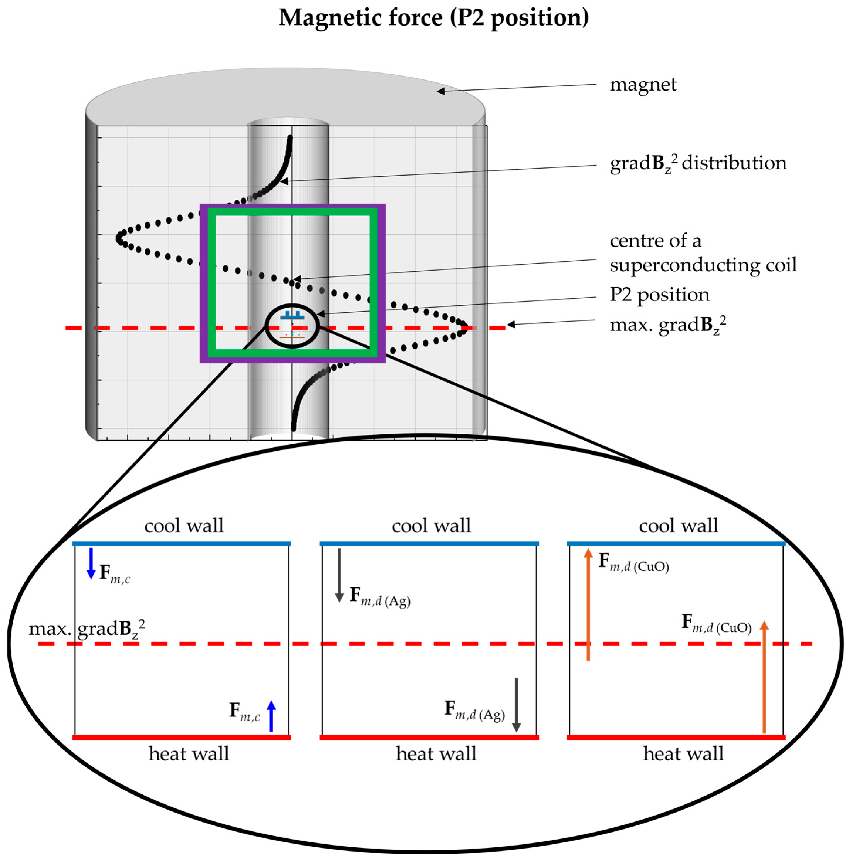
Figure 6 presents a schematic diagram of the unit magnetic force acting on the components of the nanofluids, occurring at position P2. Considering the magnetic properties and orientation of the magnetic field, it can be concluded that the magnetic buoyancy force acting on water near the cooled wall is directed downward and, near the heated wall, upward. The magnetic buoyancy force acting on Ag nanoparticles is directed downward, and the force acting on CuO nanoparticles is directed upward.

Analysing the distribution of forces during thermomagnetic convection at position P2 (diagrams in Figure 4 and Figure 6), it can be concluded that the forces acting on the water are directed in the same direction, so an intensification of thermal convection can be expected. The relationship between gravitational and magnetic forces relating to diamagnetic particles (Ag) is similar. Forces act in the same direction and orientation, so the net resultant force is directed downward. The effect may be an acceleration of downward movement and a deceleration of upward movement. For CuO particles, a different situation can be observed, namely that the magnetic force is directed upwards, so it has the opposite direction to the gravitational force, and it is noteworthy that its value is greater than that of the gravitational force. Therefore, under the right conditions, it is possible to counteract the effect of gravitational force on CuO particles. The presence of CuO particles may slightly intensify the upward movement and slightly slow the downward movement.

The final result of the interaction of forces on individual components will depend on the thermal and magnetic conditions set during the investigations and on the proportion of nanoparticles. The magnetic susceptibility of the analysed substances is relatively low, as they are weakly magnetic materials. However, as analysis has shown, it is not only the values of the forces that are important but also their direction and orientation, as well as their mutual relationship.

The net values of the forces that act on the individual phases of nanofluids, obtained from the numerical analysis, are summarised in

Table 3. Net force values obtained in theoretical and numerical analysis, unit N/m³.

	0 [T]	P1 9 [T]	P2 9 [T]
water	|10.1|	|7.7|	|12.7|
Ag0.25
carrier phase	|10.6|	|8.2|	|13.1|
dispersed phase	−257	−242	−276
CuO_0.25
carrier phase	|10.2|	|8.4|	|12.8|
dispersed phase	−159	−346	+27

for comparison purposes. The table presents data obtained for water and nanofluids containing 0.25 [vol.%] of Ag and CuO nanoparticles, without the influence of a magnetic field (0 [T]) and under the influence of a magnetic induction of 9 [T] at both studied positions of the computational domain.

To simplify the comparison of forces, they are presented as follows: the values in column ‘0 T’ correspond to the net force of gravitational buoyancy near one of the thermally active walls, while the values in the columns containing ‘9 [T]’ are the sum of the unit forces of gravitational and magnetic buoyancy near one of the thermally active walls. The ‘−’ sign next to the unit force values of the nanoparticles indicates a downward force, and ‘+’ indicates an upward force. All unit force values are expressed in N/m³.

The unit values of the forces presented in Table 3 differ slightly but are of the same order of magnitude and have similar values. More importantly, they show the same trend in value changes:

• For diamagnetic fluid (water or base fluid) at position P1, the force values decreased, and at position P2, they increased under the influence of a magnetic induction value of 9 [T];
• For diamagnetic silver nanoparticles in the upper position (P1), the net force is less negative, and in the lower position (P2), it is more negative than without the influence of the magnetic field (0 [T]);
• For paramagnetic copper oxide nanoparticles in the upper position (P1), the net force values have the highest negative value, while in the lower position (P2), they are positive, i.e., they are directed upward.

4. Global Insights

The visualisation of numerical results was prepared for water and both nanofluids: Ag0.25 and CuO_0.25 for a temperature difference of 8 [K]. Numerical calculations were performed for magnetic induction values of 0, 4, 6 and 9 [T] at positions P1 and P2 of the computational domain. To present the influence of the magnetic field, the results were selected without the magnetic field (0 [T]) and the results obtained under the action of a strong magnetic field (magnetic induction of 9 [T]) at positions P1 and P2 of the computational domain.

The results are presented in the same way for all fluids: 0 [T] (natural convection), P1 9 [T] (upper position with 9 [T] of magnetic induction), and P2 9 [T] (lower position with 9 [T] of magnetic induction).

The distributions of the following parameters were presented: temperature, velocity magnitude resulting for carrier phase with velocity vector fields of both phases (white arrows for the carrier phase—water/base fluid and black ones for the dispersed phase—nanoparticles, Ag or CuO, respectively), and vector fields of net resultant forces acting separately on the carrier phase (fluid) and separately on the dispersed phase (particles), in the corresponding colours (described above).

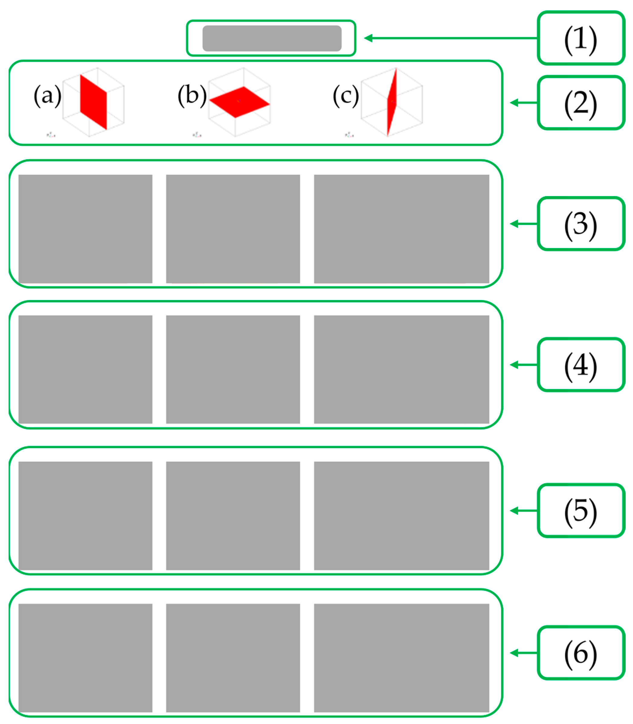
All figures have the same layout as shown in Figure 7 and contain the following:

(1)

An abbreviated title describing the fluid, temperature difference, magnetic induction value and position of the computational domain (P1 or P2, for magnetic induction equal to 9 [T]);

(2)

Schematically presented planes for which the results are presented in a given column;

(3)

Temperature distribution, together with a colour scale, in three planes;

(4)

Magnitude and vector field of velocity (white vectors, carrier phase, black—dispersed phase) with a colour scale, in three planes;

(5)

Magnitude and vector field of the net resultant force acting on the fluid (white arrows), with a colour scale, in three planes;

(6)

Magnitude and vector field of the net resultant force acting on nanoparticles (black arrows), together with a colour scale, in three planes (not applicable to water).

For results presented without the magnetic field (0 [T]), the net resultant force F_net should be understood as the gravitational buoyancy force, in the case of water, or as the gravitational buoyancy force with the interphase interaction force in the case of nanofluids. For results in a magnetic field, the resultant force is the gravitational and magnetic buoyancy forces for water, and the gravitational, magnetic and interaction forces for nanofluids can be expressed by the following equation:

$$F_{\mathrm{n}\mathrm{e}\mathrm{t}}=\left\{\begin{array}{c}{\mathbf{F}}_{g,c} \mathrm{for} \mathrm{water} \left(0\left[\mathrm{T}\right]\right)\\ {\mathbf{F}}_{g,c}+{\mathbf{F}}_{g,d}+{\mathbf{F}}_{d,c} \mathrm{for} \mathrm{nanofluids} (0 [\mathrm{T}\left]\right)\\ {\mathbf{F}}_{g,c}+{\mathbf{F}}_{m,c} \mathrm{for} \mathrm{water} \left(9\left[\mathrm{T}\right]\right)\\ {\mathbf{F}}_{g,c}+{\mathbf{F}}_{g,d}+{\mathbf{F}}_{d,c}+{\mathbf{F}}_{m,c}+{\mathbf{F}}_{m,d} \mathrm{for} \mathrm{nanofluids} (9 [\mathrm{T}\left]\right)\end{array}\right.$$

(17)

The distributions of individual parameters presented are not instantaneous values but are averaged over a period of 600 s. The selected parameter distributions are presented in three selected cross-sections to emphasise the three-dimensionality and complexity of the studied phenomena. These cross-sections are as follows: (a) a vertical plane halfway along the length of the horizontal walls, (b) a horizontal plane halfway up the cube, and (c) a diagonal plane passing through two opposite corners of the cube (schematic miniatures have been added to each result panel).

4.1. Water

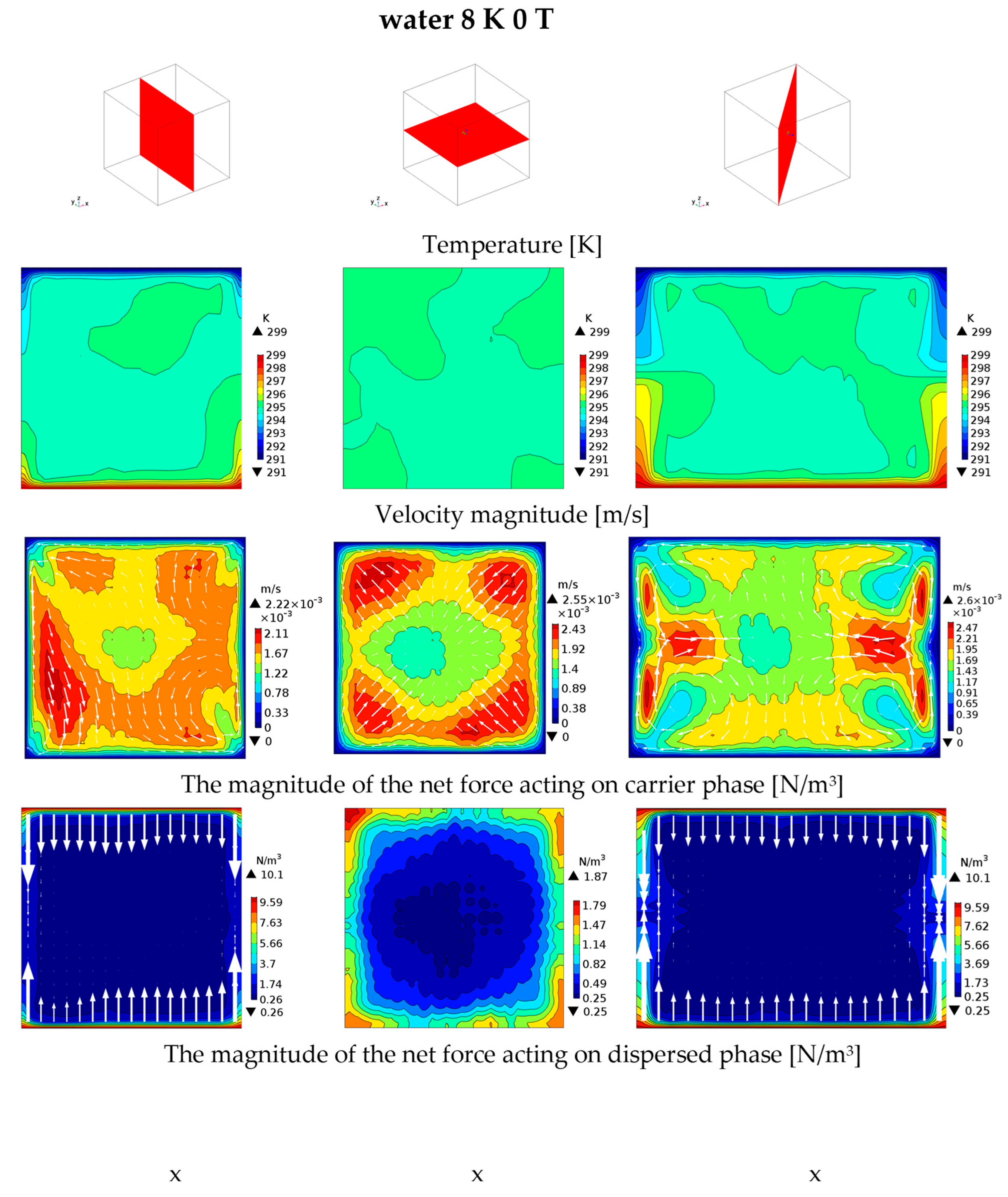
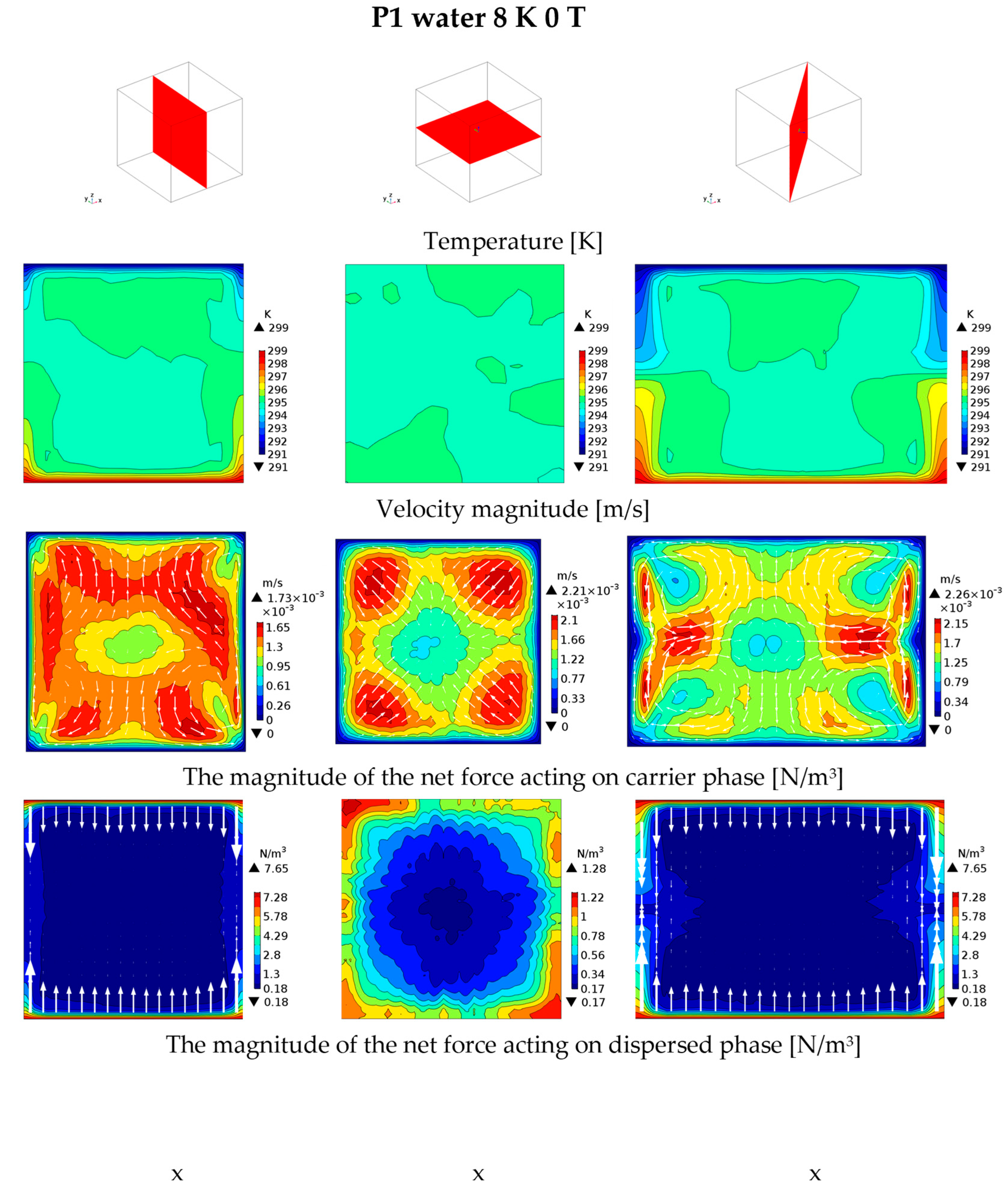
Figure 8, Figure 9 and Figure 10 show the results of numerical calculations obtained for water without a magnetic field (0 [T]) and for a magnetic induction of 9 [T] at positions P1 and P2, respectively.

In the middle zone of the enclosure, the temperature value is close to the average temperature value between the temperature values of both horizontal walls, as shown in the vertical and diagonal cross-sections. In the horizontal cross-section, located at half the height of the computational domain, the temperature distribution indicates a uniform value close to 295 [K].

The highest velocity values are located near the side walls, with the velocity vectors on the left side pointing mainly downward, while on the right side, there are two vortices, a larger one near the lower-right corner and a smaller one in the upper-right corner. In the horizontal cross-section, the fluid moves towards the centre of the cube. In the diagonal plane, a clear division into upper and lower parts can be seen. Convective motion does not cover the entire volume but occurs separately in the upper and lower parts of the cube.

Four vortex structures are also visible near the four corners, suggesting the presence of two toruses, with the slowest movement zone located in the central part of this cross-section. The symmetry of the flow can also be observed. Such a velocity field is a result of the buoyancy force, which originates from the temperature difference generated by the heated wall.

The highest values of the net resultant force are found in the close vicinity of the thermally active walls and are directed towards the centre of the enclosure. This is visible in both the vertical and diagonal cross-sections. The range of net force values is the same in both planes. Almost throughout the entire volume, the net force value is small and uniform. In the horizontal cross-section, the net force values are significantly lower, up to 2 [%] of the maximum force value compared to the other cross-sections. The highest value is located near the corners.

At position P1, under the influence of a magnetic field (magnetic induction 9 [T], Figure 9), the temperature distribution is similar to that without the influence of the field (Figure 8). The highest and lowest temperature values are located near the thermally active horizontal walls, while in the remaining area, the temperature values are uniform and close to the average. This is visible at positions P1 and P2 (Figure 10). However, a subtle difference can be observed, namely that the uniform temperature value at position P1 is lower (294 [K]) and higher (296 [K]) in position P2 compared to the absence of magnetic field influence (0 [T]). This is visible in each of the presented cross-sections. These small changes are the result of the magnetic field interaction and not temporary changes in the flow structure, as the presented values are averaged over time.

The velocity field is characterised by a larger area of high velocity values in the vertical cross-section, especially in the upper zone of the enclosure (Figure 9). Four vortices are also visible near all corners of the cross-section, resembling the structure in Figure 8.

In the horizontal cross-section, a similarity in the velocity distribution to the case without a magnetic field can be observed, with four zones of increased values of velocity and greater symmetry. The fluid moves towards the centre of the cube, which is a zone with lower velocity values. In the diagonal cross-section, there is also a similarity to the flow without a magnetic field (0 [T]). Maximum velocity values were slightly reduced from 2.6 × 10⁻³ [m/s] (0 [T] in the diagonal cross-section) to 2.3 × 10⁻³ [m/s] (also in the diagonal cross-section). In all cross-sections, greater flow symmetry and a reduction in the maximum velocity were observed as a result of the strong magnetic field in position P1.

The distribution of the net resultant force acting on the fluid also resembles that obtained without a magnetic field but is more symmetrical, especially in the vertical cross-section (Figure 9). The magnetic field stabilised the natural convection in the enclosure and caused the net force to be symmetric. The net force values are lower in the magnetic field (9 [T]) in position P1, as the maximum value is 7.65 [N/m³]. Without the influence of the magnetic field, this value was 10.1 [N/m³].

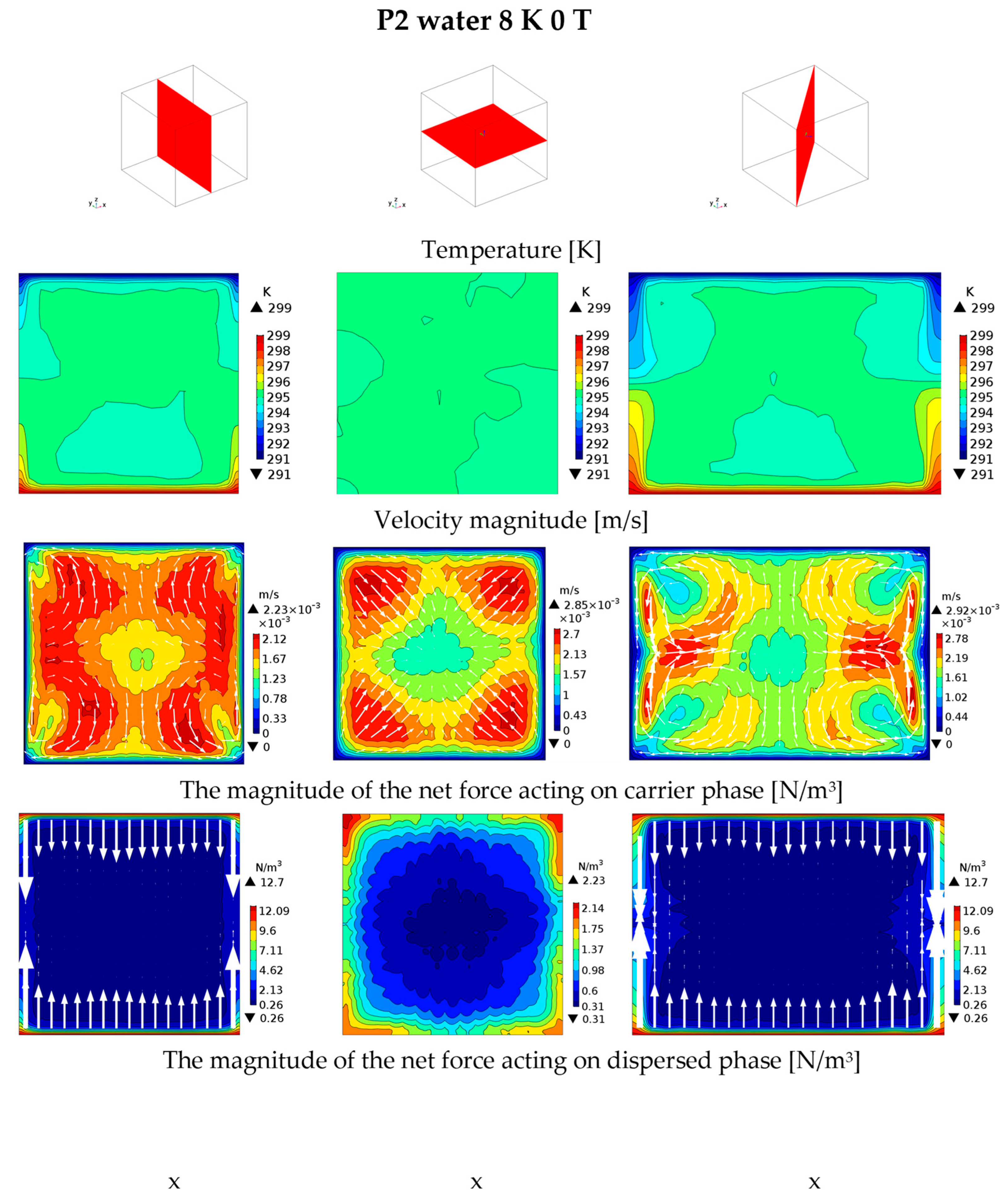
The results for water at position P2 under the action of magnetic induction with a value of 9 [T] are presented in Figure 10. The temperature distributions are similar to those of cases 0 [T] and 9 [T], P1, with warm and cold fluid zones located near the horizontal walls, but the temperature value in the central zone of the enclosure is higher, about 295.5–296 [K]. The fluid motion has a structure similar to that without a magnetic field. The structure and direction of the fluid are symmetrical and have not been modified by the magnetic field. An increase in the areas with the highest velocity values can be observed, and the maximum velocity value increased to 2.9 × 10⁻³ [m/s] after applying a strong magnetic field in position P2.

The distribution of the net resultant force acting on the fluid is symmetric in each of the cross-sections presented. Net force values are greater than in the case without the application of a magnetic field and for position P1 after the application of a magnetic induction of 9 [T]. In this case, the magnetic force enhanced natural convection through strengthening the gravitational force. The maximum net force value at position P2 was 12.7 [N/m³]. The magnetic field contributed to the homogenisation of the flow structure and force distribution, regardless of the position of the computational domain.

In position P1, the values of the net force acting on the fluid and the velocities are lower. On the contrary, at position P2, the trend reverses, with higher values of net force and velocity.

4.2. Silver Nanofluid

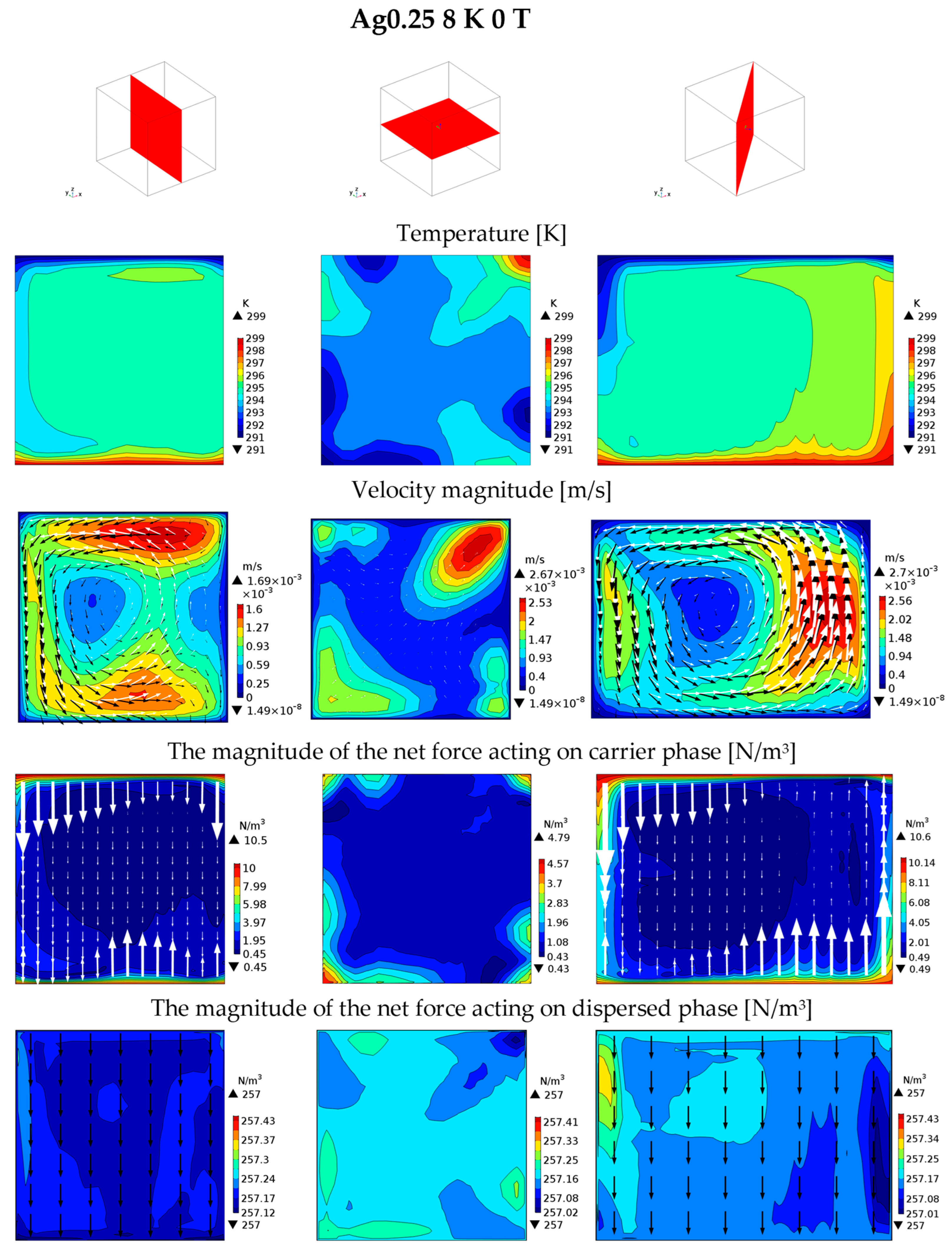
The results for Ag0.25 nanofluid are presented in Figure 11, Figure 12 and Figure 13, respectively, without a magnetic field (0 [T]) and for a magnetic induction of 9 [T] in positions P1 and P2. The temperature distribution for Ag0.25 is more complex, with a stream of cold fluid near the left wall. In the diagonal cross-section, the contours with the highest values are on the right and the lowest on the left. Compared to water (0 [T]), the fluid in the central zone of the enclosure has a lower temperature. There is one large vortex structure moving counterclockwise in both vertical and diagonal cross-sections, which is the dominant direction of movement in the analysed system.

The horizontal cross-section shows an area of higher velocity values (red colour in the upper-right corner) and a large area where the values of velocity are low or close to zero. The velocity vectors are invisible, which is caused by the fluid moving perpendicular to this plane. Considering the velocity distribution in all the cross-sections presented, the highest velocity values are achieved by the fluid moving upward (white vectors) and the nanoparticles moving downward (black vectors). In certain areas, differences can be seen in the movement of the fluid and nanoparticles. Near the horizontal walls, the vectors representing the nanoparticles deflect more downward than the vectors representing the fluid. This is the result of a gravitational force acting on the particles and orienting them downward. The nanoparticles are influenced by the movement of fluid but also “pulled down” by the gravitational force. The fluid velocity values in the vertical cross-section are the lowest (also lower than the water velocity, 0 [T], Figure 8). On the contrary, in the horizontal and diagonal cross-sections, the maximum fluid velocity values are similar and equal to approximately 2.7 × 10⁻³ [m/s].

The velocity distribution is the result of gravitational forces acting on both components of the nanofluid. Their opposite directions at various locations in the enclosure caused differences in the velocity distribution. The distribution of the net resultant force acting on the fluid reflects the temperature distribution. The net force is directed vertically (upward or downward), which is why no vectors are visible in the horizontal cross-section. An increase in the net force acting on the fluid can be observed, compared to water tested without a magnetic field, from 10.1 to 10.5 [N/m³] in the vertical cross-section and similarly in the diagonal cross-section. The lowest net force value is visible in the horizontal cross-section but with the largest increase in its maximum value from 1.9 (for water (0 [T])) to 4.9 [N/m³]. The distribution of the net resultant force acting on the nanoparticles is uniform, with values ranging from 257 to 257.5 [N/m³]. Therefore, it can be said that this is approximately a constant value. The net force acting on the particles is many-times greater than the net force acting on the fluid, but the concentration of nanoparticles is relatively small. The net resultant force acting on the nanoparticles is directed downward, which is the effect of the gravitational force and the interfacial interaction force (which has a small value). This increases the velocity with which the nanoparticles move downward.

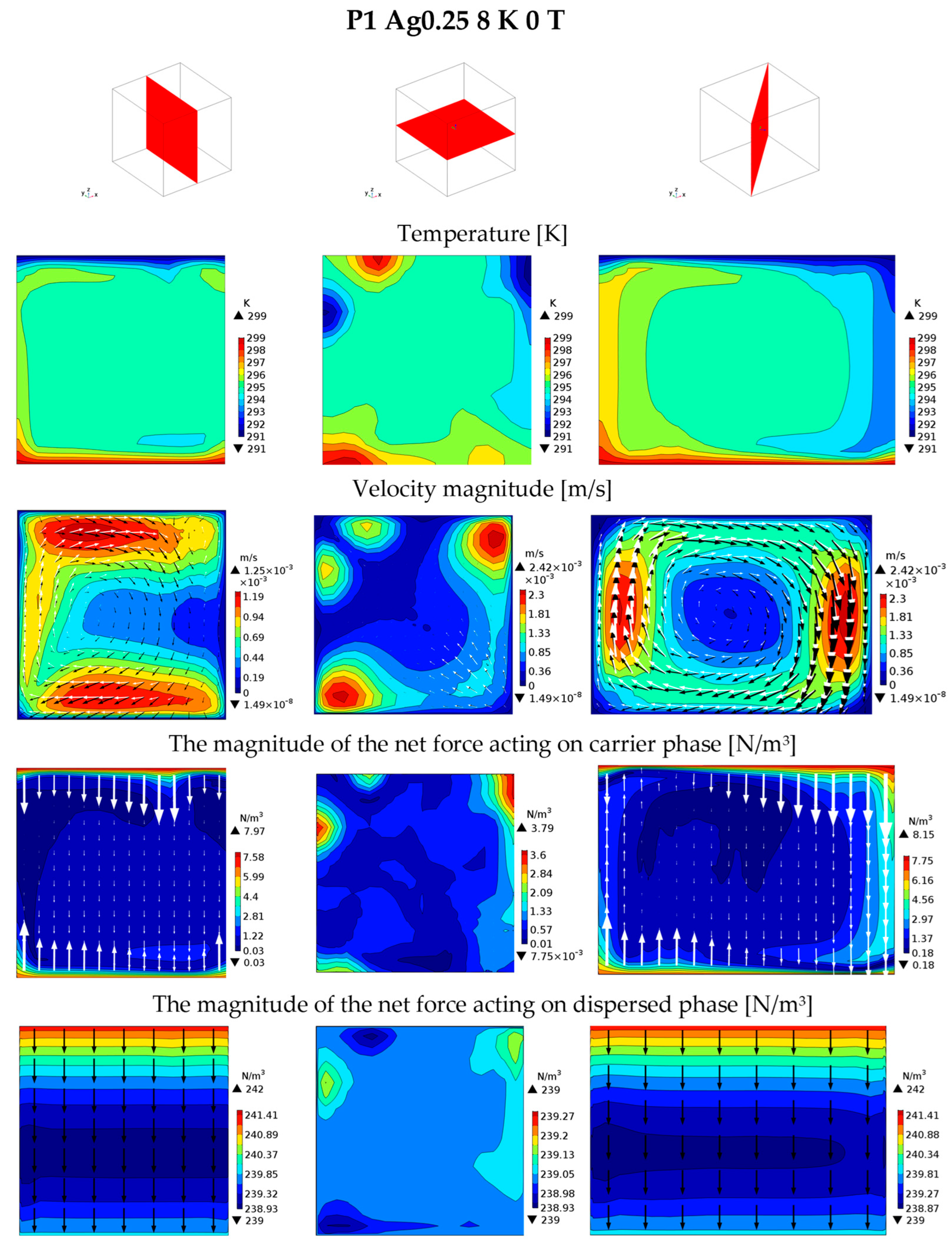
The results of numerical calculations for the Ag0.25 nanofluid under the action of magnetic induction with a value of 9 [T] in position P1 are presented in Figure 12. The highest and lowest temperature values are located near the heated and cooled walls, respectively, and are visible in the temperature distributions in the vertical and diagonal cross-sections. A change in the position of the warm and cold fluid streams can be observed compared to the distribution without a magnetic field (Ag0.25, 0 [T]).

The velocity vectors of both phases, visible in the velocity distributions, indicate a change in the main direction of movement to clockwise. Single, large vortex structures are visible in the vertical and diagonal cross-sections. The reason was the appearance of magnetic forces acting on both components of nanofluid, but the biggest impact was observed in fluid behaviour, changing the direction of movement. The zones of the highest velocity values are located near the horizontal walls in the vertical cross-section and near the horizontal walls in the diagonal cross-section. In this case, too, it can be seen that the velocity values of the nanoparticles increased during downward movement (black vectors) and that of the fluid during upward movement (white vectors). During horizontal movement, the velocity vectors for the dispersed phase (black) deviate downward. It was caused by the combined gravitational and magnetic forces acting on them in the same direction. The velocity values in position P1 are lower than in the case without a magnetic field. The maximum velocity value in the vertical cross-section decreased from 1.7 × 10⁻³ to 1.25 × 10⁻³ [m/s] and in the horizontal and diagonal cross-sections from 2.7 × 10⁻³ to 2.4 × 10⁻³ [m/s]. However, the velocity values of the nanofluid are higher than those of water in a similar position under the influence of a magnetic field (P1, water, 9 [T], Figure 9), which were approximately 2.3 × 10⁻³ [m/s] at maximum.

The distribution of the net force acting on the fluid has not changed significantly. However, in the diagonal plane, the highest net force values are in line with the direction of movement caused by the magnetic field. The application of the magnetic field also reduced the net force acting on the fluid. The maximum values of the net force acting on the fluid were reduced after applying the magnetic field from 10.6 to 8.2 [N/m³]. In turn, the distribution of the force acting on the nanoparticles differs significantly in a magnetic field from that in the case without its application (0 [T]). A horizontal distribution of its values is visible, which results from the distribution of the magnetic induction gradient square (gradB_z²) (Figure 2, right side). The net resultant force ranges from 239 to 242 [N/m³], and, therefore, these values are lower than without the influence of the magnetic field (0 [T]).

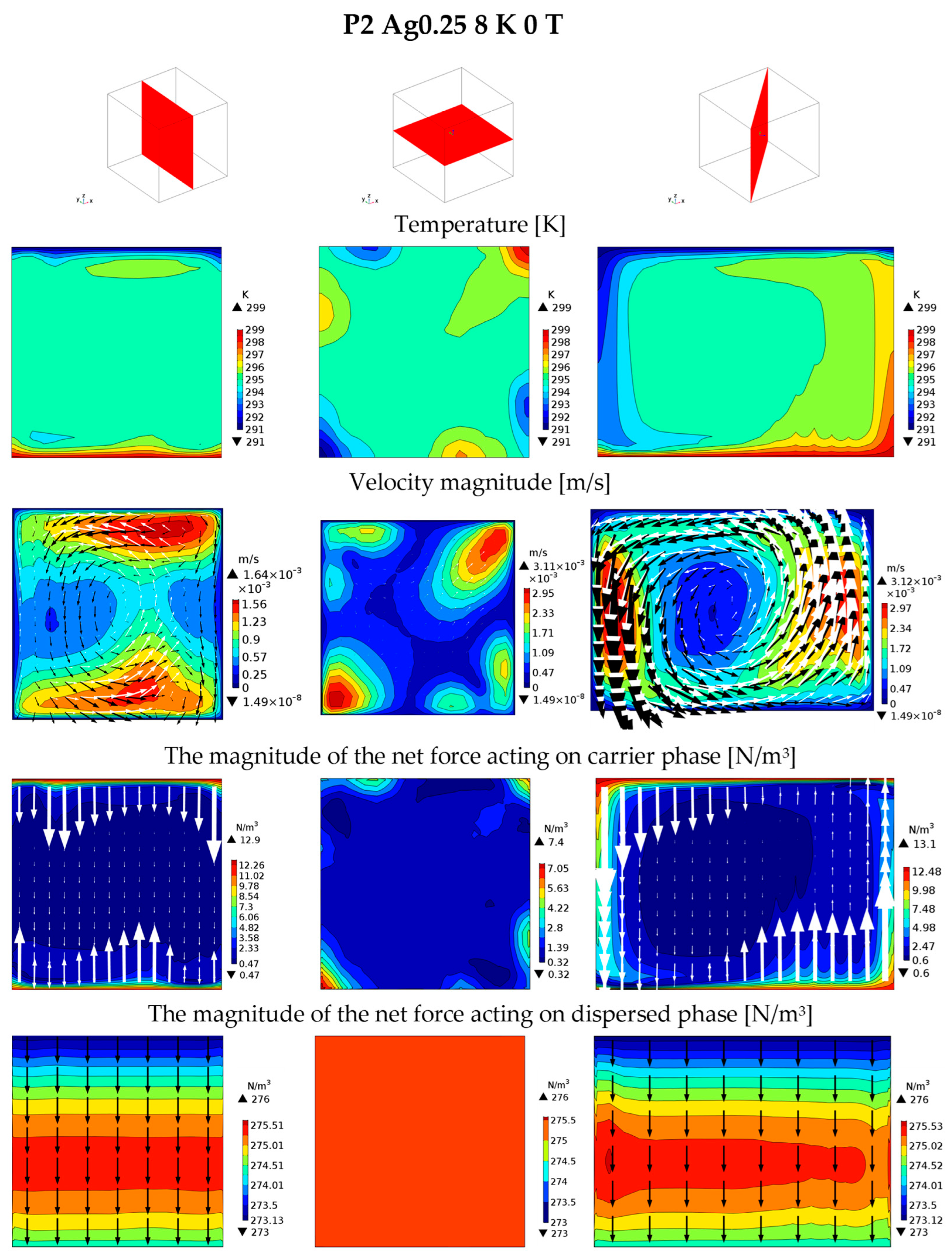
The results of the numerical calculations for Ag0.25 nanofluid under the action of a magnetic induction of 9 [T], in position P2, are presented in Figure 13. The temperature distribution is similar to that obtained for 0 [T], but the temperature distribution in the centre of the domain is more uniform and its value is higher, approx. 295 [K].

The velocity distribution is also very similar to that without the magnetic field. The same direction and counterclockwise rotation of the fluid are visible. The zones of higher fluid velocity (white vectors) and nanoparticles (black vectors) are even more clearly visible. The higher velocity of the nanoparticles was found on the left-hand side, which is consistent with the stronger net force acting on them. The net force acting in the fluid is very similar on both sides of the enclosure; therefore, the fluid velocity vectors were almost equal in magnitude in these regions. In the horizontal cross-section, six areas with higher fluid velocity values can be distinguished. They suggest the presence of more than one vortex structure in the system, with the main and dominant one being the one shown in the diagonal cross-section with the highest velocity values. The velocity vectors are not visible in the horizontal cross-section because the motion is perpendicular to it (as it would be without the magnetic field). The maximum velocity increased as a result of the magnetic field interaction from 2.7 × 10⁻³ to 3.1 × 10⁻³ [m/s] in the diagonal and horizontal cross-sections, while in the vertical cross-section, the velocity values are similar to those without its application. The maximum velocity values for Ag0.25 nanofluid are higher than for the analogous position for water, with less variation in velocity in individual cross-sections for water.

The distribution of the net resultant force acting on the fluid is similar to that in the absence of a magnetic field in each cross-section and resembles the temperature distribution. The highest net force values occur in the upper-left and lower-right corners of the diagonal cross-section. The maximum force value increased from 10.6 to 13.1 [N/m³] after applying a magnetic field with a magnetic induction of 9 [T]. The distribution of the resultant net force acting on the nanoparticles, similar to the P1 position, is characterised by a horizontal distribution of values. However, in position P2, the highest net force value is located near the middle of the enclosure height, which is consistent with the maximum value of gradB_z², which is positive in position P2. The values of the net resultant force acting on Ag nanoparticles range from 273 to 276 N/m³ and are greater than the force value without the application of a magnetic field (0 [T]).

4.3. Copper Oxide Nanofluid

The visualisation of the numerical results obtained for CuO_0.25, respectively, without a magnetic field (0 [T]) and for a magnetic induction of 9 T at positions P1 and P2 of the calculation domain, is presented in Figure 14, Figure 15 and Figure 16.

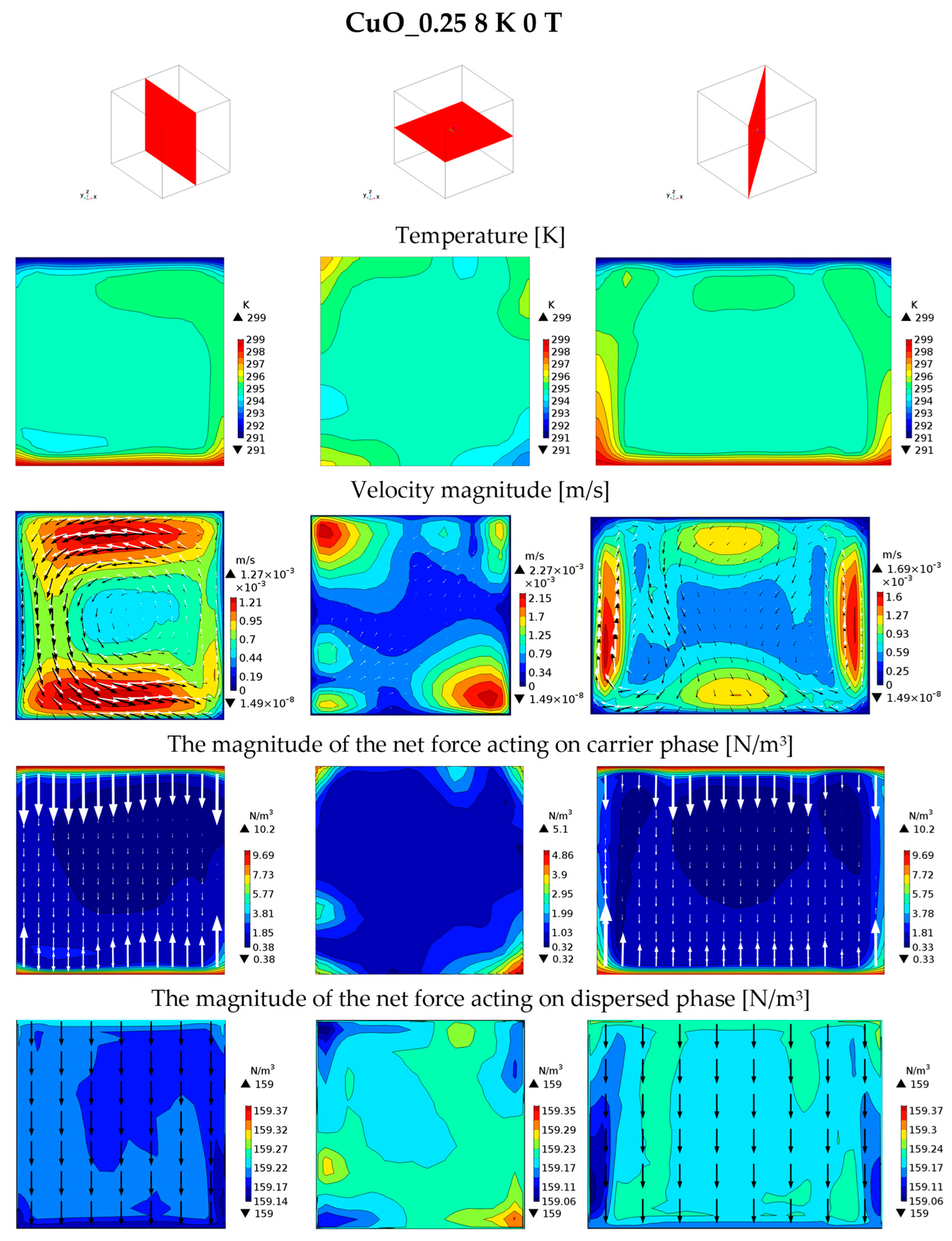
The temperature distribution is more similar to that presented for water (0 [T], Figure 8) than for Ag0.25 nanofluid (0 [T], Figure 11). The highest and lowest temperature values are located near the thermally active walls (heated and cooled), which is visible in the vertical and diagonal cross-sections. However, the temperature distribution in the central zone of the enclosure is more uniform.

The velocity distribution in the vertical cross-section is not similar to that for water (0 [T]); it is more similar to the distribution presented for Ag0.25 nanofluid (0 [T]), as there is a single vortex covering the entire visible space. The fluid moves clockwise. In contrast, in the diagonal cross-section, the velocity distribution indicates a complex flow structure with two vortices. Such a structure, governed by the gravitational forces acting on the nanoparticles and fluid, indicated weak natural convection. In the horizontal cross-section, two zones with maximum velocity values and four zones with higher velocity values are visible. The maximum velocity value of 2.8 × 10⁻³ [m/s] is higher than that obtained for water (0 [T]) and similar to the velocity value recorded in the flow of Ag0.25 nanofluid (0 [T]).

The distribution of the net resultant force acting on the fluid is related to the temperature distribution, with the maximum force values occurring near the horizontal, thermally active walls. The maximum value of net force is 10.2 [N/m³], which is close to the value obtained for water (10.1 [N/m³]) and less than the maximum value obtained for Ag0.25 nanofluid (10.6 [N/m³]). The value of the net resultant force acting on CuO nanoparticles ranges from 159 to 159.4 [N/m³], which can be considered a constant value. The net force acting on the CuO nanoparticles is directed downward (toward the heated wall), as in the case of the Ag nanoparticles, but its value is lower than that (for the Ag nanoparticles, this value was close to 257 [N/m³]). This is due to the difference in properties because the density of Ag is greater than that of CuO.

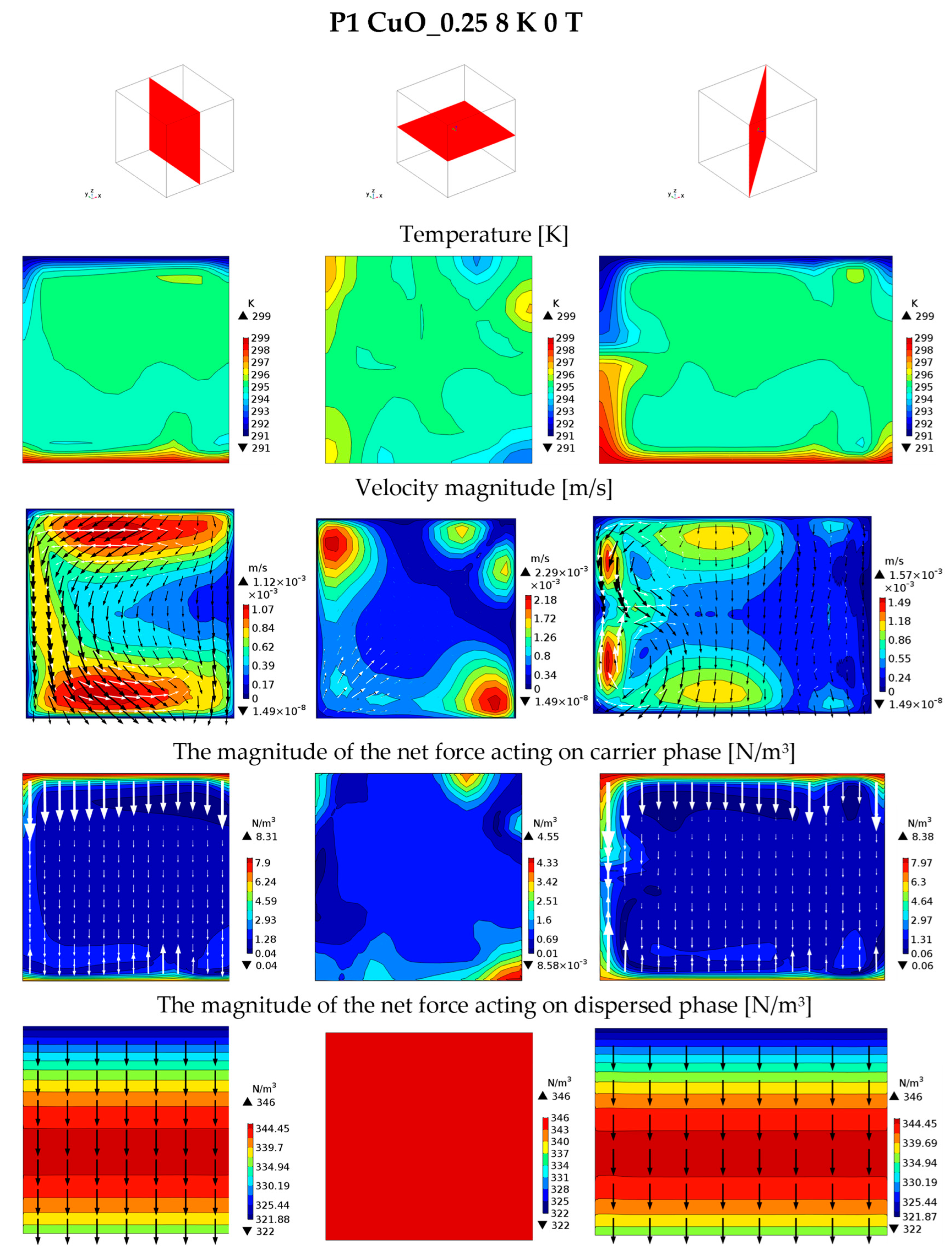
Figure 15 shows the results for the CuO_0.25 nanofluid after applying a magnetic field with a magnetic induction of 9 [T] at position P1. The temperature distribution resembles that obtained without the influence of the magnetic field (0 [T]). However, the temperature value in the central zone of the enclosure is higher compared to the case without a magnetic field. Additionally, in the diagonal cross-section, there is no symmetry in the temperature values, as without the application of a magnetic field.

In the vertical cross-section, the same direction of fluid movement can be observed, as well as two zones with higher velocity values, located in the same areas as without the influence of the magnetic field; however, the velocity value was slightly reduced. The horizontal cross-section shows a small area occupied by white vectors (carrier phase), indicating horizontal fluid movement. The black vectors (dispersed phase) are not visible, suggesting vertical movement of the nanoparticles, which is governed mostly by gravitational forces. On the left side, a complex flow structure is visible. Halfway up the wall, there is a horizontal movement of the carrier phase, and a small vortex is also visible in the lower-left part of the cross-section. The maximum velocity values are similar to those without a magnetic field. This may only indicate the reorganising effect of the magnetic field on the flow for this type of nanofluid in position P1 (diamagnetic fluid—paramagnetic nanoparticles).

The distribution of the net resultant force on the fluid reflects the temperature distribution in individual cross-sections. However, it can be seen that higher net force values are visible in the upper part of the domain, near the cooled wall, directed downwards. The maximum value of the net force acting on the fluid decreased from 10.2 to 8.4 [N/m³] as a result of the magnetic field at position P1. Thus, the magnetic field in this position of the domain has a slowing effect on the phenomenon of convection, which is also confirmed by the smaller velocity values. The maximum values of the net force acting on the fluid are similar to those obtained for Ag0.25 (Figure 12) and are slightly higher than the values obtained for water (water 9 [T], Figure 9) at the analogous position P1. The distribution of the net resultant force acting on the nanoparticles is characterised by a horizontal arrangement of contours, in accordance with the gradB_z² distribution (Figure 2, right side), with the maximum value located approximately halfway up the computational domain.

The effect of the magnetic field is different from that for Ag nanoparticles (P1 Ag0.25 9 [T]), which are diamagnetic. On CuO nanoparticles, which are paramagnetic, the magnetic field acts attractively, i.e., the net force is directed towards the highest magnetic induction value. The resultant force on the nanoparticles increased, and it is twice as high as in the case without a magnetic field.

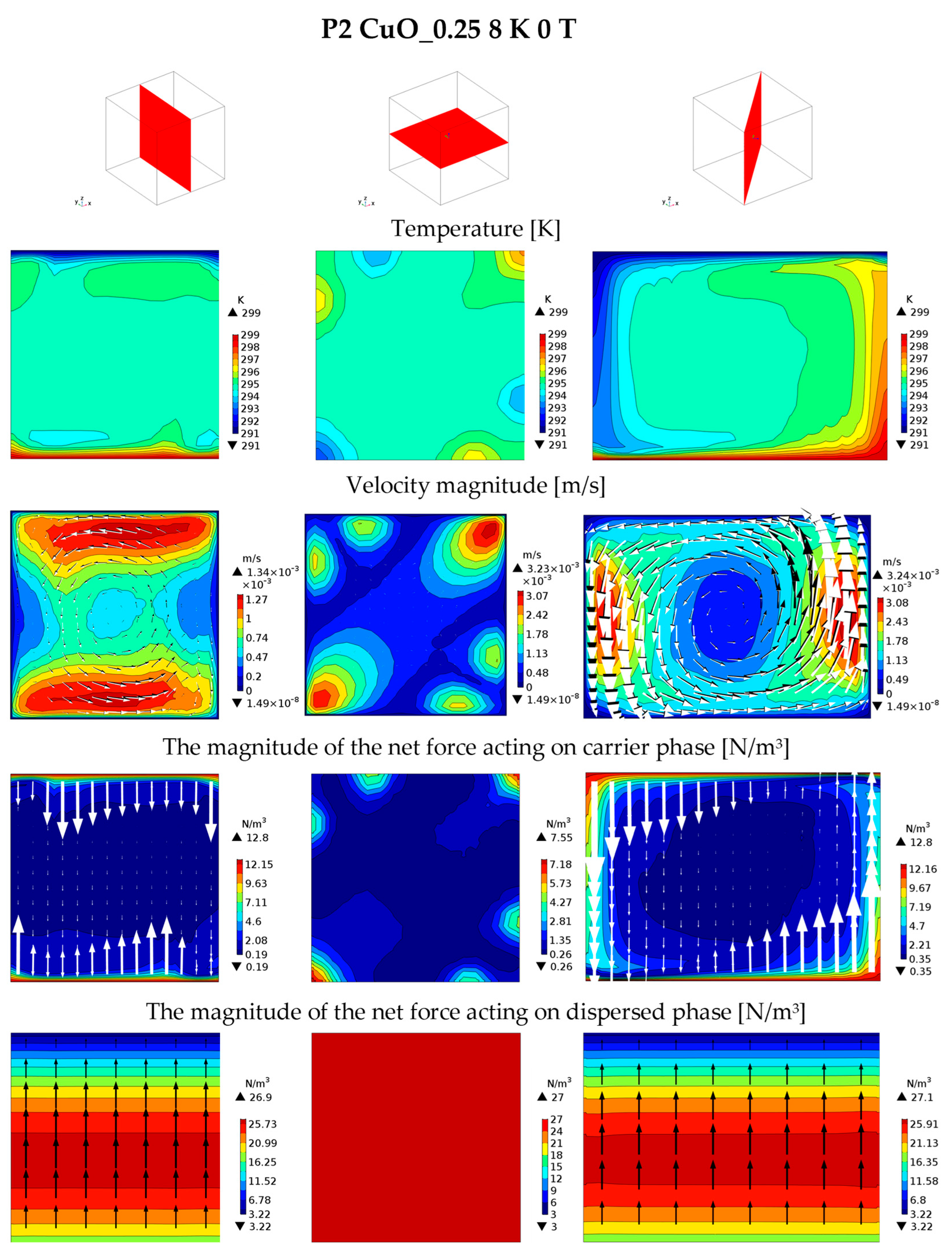
The temperature distribution obtained for CuO_0.25 at position P2 under the action of a magnetic induction of 9 T in the vertical cross-section resembles that obtained without a magnetic field (0 [T], Figure 16). However, the horizontal and diagonal cross-sections show a temperature distribution different from that obtained without the influence of magnetic induction. In the horizontal cross-section, six areas with temperatures different from the average value can be observed. They are symmetrical along the diagonal. This suggests a counterclockwise movement in the diagonal cross-section.

The diagonal cross-section shows a large vortex structure covering almost the entire space presented. The fluid moves in a counterclockwise direction. The velocity vectors representing the base fluid (white) are longer than those representing the nanoparticles (black vectors), both when the flow is directed upward and downward. It is due to a summation of the gravitational and magnetic forces acting on the fluid. In addition, the vectors representing CuO nanoparticles do not deviate downward when the direction of movement is horizontal but, rather, deviate slightly upward, which was caused by the magnetic force acting on them.

This phenomenon has not been observed in other cases, even without the application of a magnetic field. The reason for this relationship between phase velocities and the deviation of the dispersed phase vectors, which is different from what has been observed so far, is the application of a strong magnetic field. The maximum velocity values occur in the horizontal and diagonal planes and are identified with the dominant vortex structure in the system. The maximum velocity of 3.24 × 10⁻³ [m/s] is the highest velocity value among all the presented cases.

The distribution of the net value of the resultant force acting on the fluid, as in previous cases, reflects the temperature distribution. The net force vectors are vertical and, therefore, not visible in the horizontal cross-section (middle column). The maximum value of the net force acting on the fluid, for a nanofluid containing 0.25% by volume of CuO particles, increased as a result of the action of a magnetic field with a magnetic induction of 9 [T] at position P2 to 12.8 [N/m³], compared to the value of 10.2 [N/m³] obtained without the application of a magnetic field.

The distribution of the net resultant force acting on nanoparticles in the magnetic field at position P2 initially resembles that obtained for the upper position (P1, 9 [T]). A horizontal distribution of its values is visible, analogous to the gradB_z² distribution, with the highest value visible near the middle of the computational domain. However, this is where the similarities end. The value of the net resultant force is the smallest of all the values presented (in the case of Ag, in both positions of the computational domain, and on CuO at position P1) and amounts to approximately 27 [N/m³].

The most interesting effect of the magnetic field can also be observed: the net magnetic force acting on CuO nanoparticles (paramagnetic particles) acts in the direction of the highest magnetic induction values, i.e., for position P2, it is directed upward. It determined the direction of the net resultant force. This is the only case where the magnetic force changed the direction of the net resultant force acting on the nanoparticles. This is the reason for the different phase velocity relationship than before.

It has been demonstrated that the effect of a magnetic field on CuO particles is significantly greater than that of Ag particles, even though both types of particles are present in the same concentration in the nanofluids. This effect is explained by their different physical properties, in particular their magnetic susceptibility, which has a consequence on the values of the force. For CuO, the magnetic susceptibility value is an order of magnitude higher and is positive.

5. Flow Dynamics

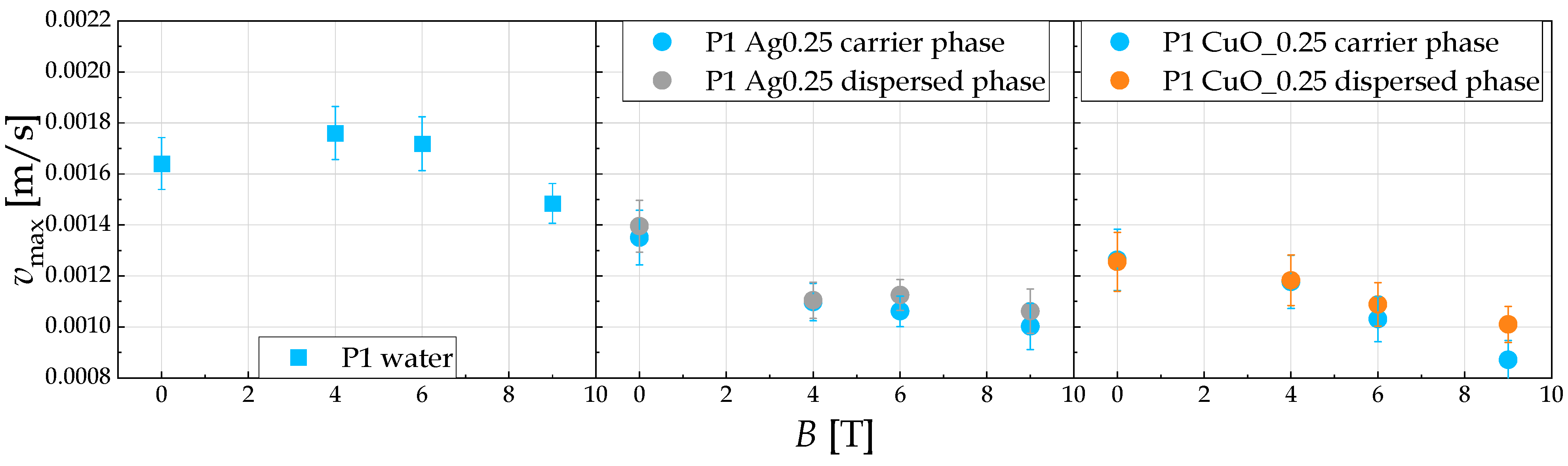
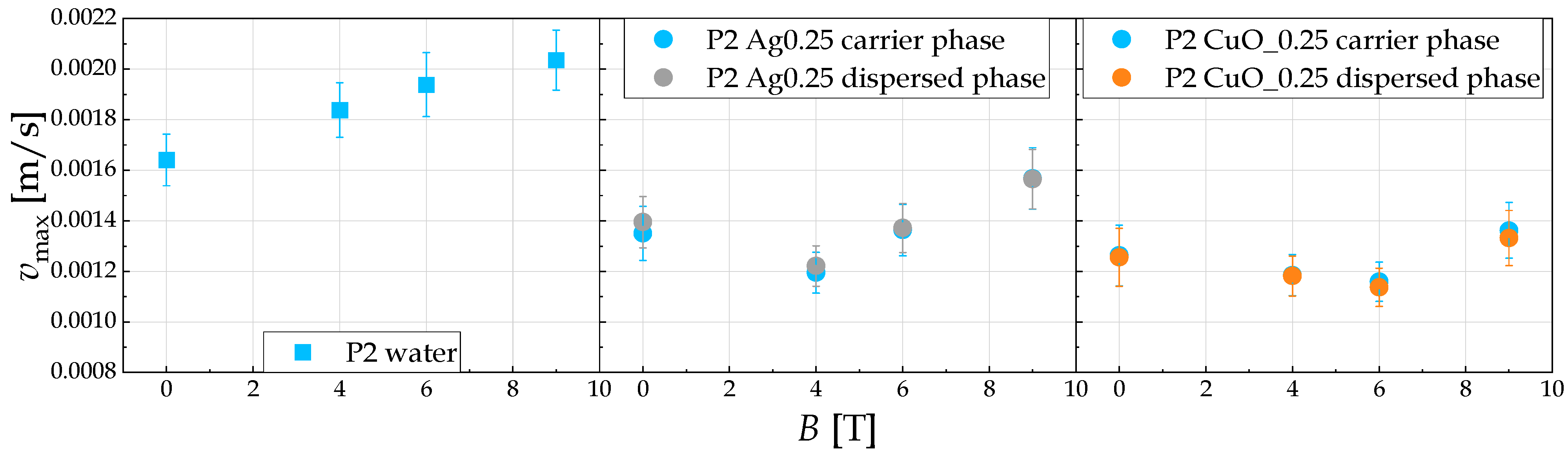
The numerical results obtained allowed us to determine the maximum velocity values that occur in the cases analysed, which are presented in Figure 17. In position P1, the maximum velocity value for water increases at 4 [T], then decreases, and at 9 [T], it is lower than without the influence of the magnetic field (0 [T]). For Ag0.25 nanofluid, the velocity values of the nanoparticles (grey) are higher than for the base fluid (blue), but both values decrease with increasing magnetic induction. A similar trend can be observed for the CuO_0.25 nanofluid, with the velocity values of the fluid (blue) and nanoparticles (orange) being very similar for magnetic inductions of 0 and 4 [T]. The maximum velocity values without the application of a magnetic field are lower for nanofluids than those of water, with the lowest value determined for the CuO nanofluid.

The velocity values for position P2 are shown in Figure 18. For water, an upward trend is visible: the higher the magnetic induction value, the higher the fluid velocity. Ag nanoparticles in Ag0.25 nanofluid (grey) have a very similar velocity value to the base fluid throughout the entire magnetic induction range, and at higher magnetic induction values, the values are almost identical. The velocity value at 4 [T] decreases, whereas at higher magnetic induction values, it increases to values higher than without a magnetic field. On the contrary, for the CuO nanofluid, the velocity values of both phases are almost the same for low magnetic induction values (0 and 4 [T]), while for 6 and 9 [T], the fluid velocity value is higher than that of the nanoparticles. The uncertainty in the calculations was expressed as the standard deviation of the velocity from the maximum value in the entire volume and averaged over time (600 [s]) and shown in Figure 17 and Figure 18 as error bars.

6. Heat Transfer

When the effects of the magnetic field on the two nanofluids are compared, it can be said that in the case of the Ag0.25 fluid, the effect is more subtle, although it is noticeable. At the same time, in the case of the CuO_0.25 nanofluid, the effect is well visible, and there is a complete rearrangement of the flow structure. For both Ag0.25 and CuO_0.25, the most obvious effect is seen in terms of velocity at position P2. This is also evident in the results of heat transfer processes as an increase in the Nu/Nu_0T ratio.

After a deep analysis of the heat transfer numerical results, correlations describing the variability in the Nusselt number were proposed. Nusselt number correlations take into account parameters such as the previously defined thermomagnetic Rayleigh number (Ra_TM), the nanoparticle concentration (φ) and their magnetic susceptibility (χ_d). The following are the proposed equations:

• For water:

$${\mathrm{N}\mathrm{u}}_k=0.27·{{\mathrm{R}\mathrm{a}}_{\mathrm{T}\mathrm{M}}}^{0.25}$$

(18)

• For nanofluids:

$${\mathrm{N}\mathrm{u}}_k={{\mathrm{R}\mathrm{a}}_{\mathrm{T}\mathrm{M}}}^{0.25}·f^{0.28}·{\left|{\chi }_d\right|}^{-0.025}$$

(19)

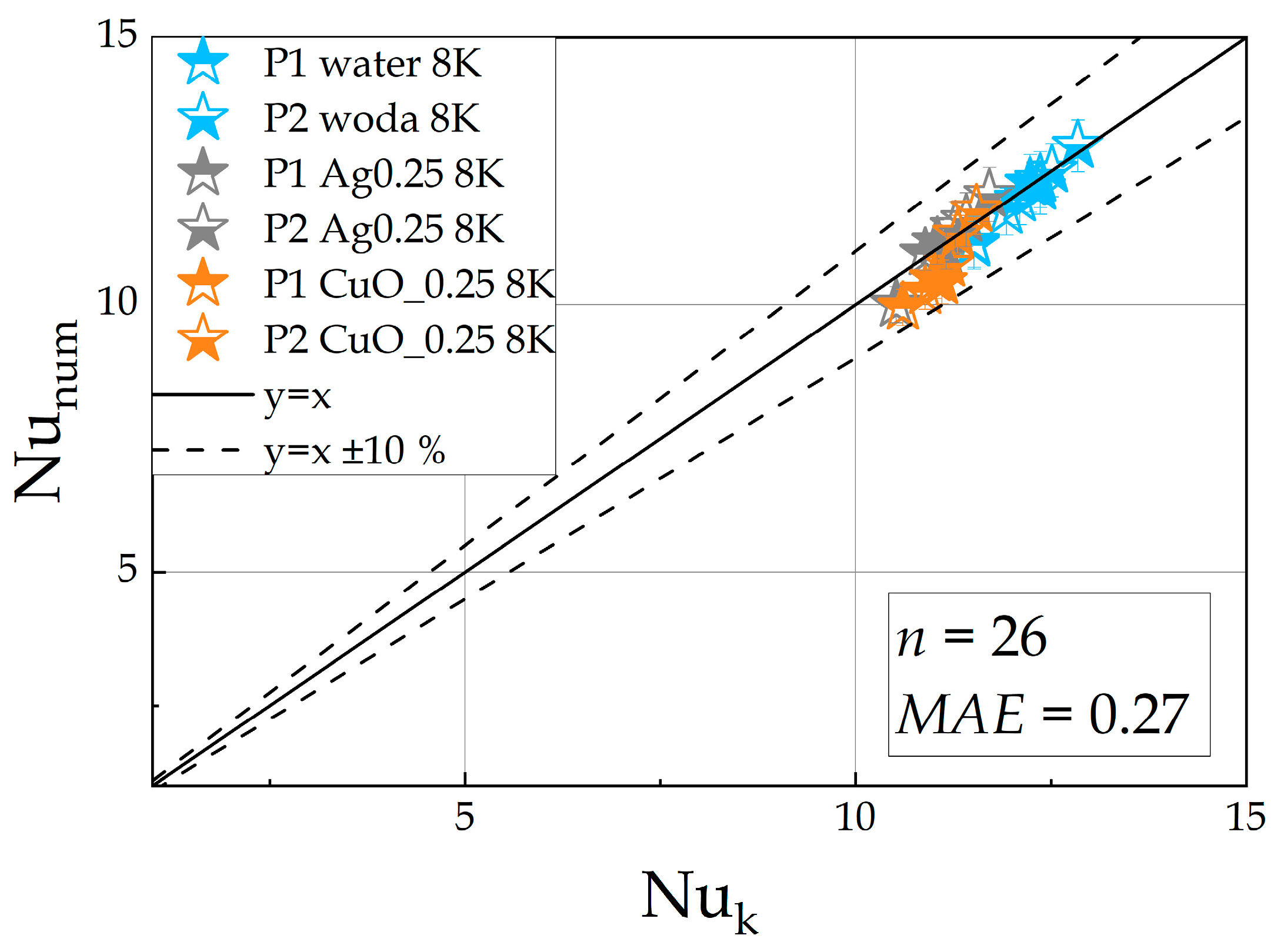
Figure 19 presents the numerically obtained Nusselt number values (Nu_num) compared to the Nusselt number values (Nu_k) calculated from Equations (18) and (19). The range of variation (±10 [%]) is also marked with dashed lines. The values obtained for positions P1 and P2 are in good agreement.

The Mean Absolute Error (MAE) was calculated to quantify the deviation of the proposed correlation of the Nusselt number from the numerical results, which were the reference data, accordingly:

$$MAE= {\displaystyle \frac{1}{n}}{\sum }_{i=1}^n\left|{\mathrm{N}\mathrm{u}}_k-{\mathrm{N}\mathrm{u}}_{num}\right|$$

(20)

The updated Figure 19 includes a statistical summary box reflecting the number of data points (equal to 26) and the MAE value (equal to 0.27) and quantifies the average magnitude of the errors in the units of the Nusselt number. These values allow for a direct assessment of the performance of the model.

Additionally, the Mean Absolute Percentage Error (MAPE) was included to provide a clearer view of the relative accuracy. The calculated value was 2.54 [%], which demonstrates the high relative accuracy of the model. To ensure statistical correlation, a Shapiro–Wilk normality test [13] was performed on the residuals. The resulting p−Value of 0.094 confirms (see

Table 4. The results of the Shapiro–Wilk test.

DF	Statistic	p-Value	Decision at Level (5%)
26	0.93349	0.09388	Cannot reject normality

) that the errors follow a normal distribution (the hypothesis of normality cannot be rejected), indicating the absence of systematic bias in the proposed model.

The number of datapoints and MAE has been added to the plot. The correlation was determined for the following parameter ranges: Ra_TM from 3.2 × 10⁶ to 5.4 × 10⁶, magnetic induction in the range of 0 to 9 [T], and a concentration of silver and copper oxide nanoparticles of 0.25 [vol.%]. Magnetic susceptibility was constant for both investigated nanofluids. The much lower value of magnetic susceptibility does not interfere with natural convection heat transfer intensity; a much higher value significantly reduces or enhances natural convection (depending on the position in the magnetic field).

7. Summary

The main goal of the presented research was to quantitively verify whether a strong magnetic field would be able to enhance or attenuate heat transfer processes in the case of thermal convection. Therefore, the thermomagnetic convection of weakly magnetic nanofluid was under investigation. The studies included a number of parameters, such as magnetic conditions, nanoparticle material, and nanofluid components’ magnetic characteristics of the components of nanofluids. Combining all considered aspects led to a complex system that provided knowledge of heat transfer processes, but deeper analyses of the flow structure and forces’ system allowed for their clarification.

It should be emphasised once again that the thermophysical properties of the analysed nanofluids are extremely important, and in the case of thermomagnetic convection, the magnetic properties are the most important among them. In position P1, the interaction of forces indicates a decrease in heat transfer for a diamagnetic fluid. For all fluids analysed, convection attenuation was observed at this position, with the highest attenuation achieved for water and Ag0.25, which shows that the addition of CuO nanoparticles had a slight enhancing effect. At position P2, theoretical analysis indicated that the most expected effect of the magnetic field would be an intensification of heat transfer (expressed by a higher Nusselt number). For all fluids analysed, an enhancement in convection was obtained in this position. However, it should be noted that the results obtained for Ag0.25 (10 [%]) are higher than those for water (6 [%]), and the results for CuO are the highest (13 [%]). This shows that the addition of both types of nanoparticles had a positive effect, but CuO had the highest effect.

Based on the presented research, a clear difference in the effect of the magnetic field on individual fluids (distilled water, nanofluid containing Ag nanoparticles and nanofluid with CuO nanoparticles) was demonstrated in the analysis of forces acting in the system, heat transfer analysis and flow structure, which results from the different magnetic properties of their components. This confirms the conclusion that the flow of nanofluids in a magnetic field should be treated as a multiphase flow, and that the presence of nanoparticles is crucial and cannot be ignored (e.g., by averaging the properties of the base fluid and nanoparticles).

These insights have great potential for engineering applications, especially in the design of advanced magnetic cooling systems for high-performance electronic devices or energy converters, where traditional gravity-driven convection is insufficient. The research provides practical guidance on magnetic field configuration: Position P2 (where the magnetic force is consistent with gravitational one and supports the buoyancy flow) should be used in compact heat exchangers to actively increase heat dissipation. On the contrary, position P1 can be intentionally used in processes that require controlled heat transfer attenuation or flow stability. Furthermore, the results suggest that in the systems requiring maximum thermal performance, such as focused cooling in microelectronics, paramagnetic nanoparticles (such as CuO) should be preferred over diamagnetic ones (such as Ag) to maximise the effect of external magnetic field intensification.

Based on the results, it was possible to formulate the Nusselt number correlation for water-based nanofluids Ag0.25 and CuO_0.25. The correlation is restricted to the ranges of parameters: thermomagnetic Rayleigh number, magnetic induction, and concentration of the particles.

It should be mentioned that the correlation integrates the thermomagnetic Rayleigh number, the nanoparticle concentration, and their magnetic susceptibility. In the literature, there are no reports discussing this problem. It is a first attempt toward a compact description of complex phenomena and their quantitative contribution to the overall effect of heat transfer. The agreement between the Nusselt value data and the proposed expression is within a ±10 [%] range. The correlation can be applied in the prediction of the thermal effect of magnetic field presence, for the verification of numerical models and extension of the analyses.

References

1. Cardoso, B.D.; Souza, A.; Nobrega, G.; Afonso, I.S.; Neves, L.B.; Faria, C.; Ribeiro, J.; Lima, R.A. Progress in Nanofluid Technology: From Conventional to Green Nanofluids for Biomedical, Heat Transfer, and Machining Applications. Nanomaterials 2025, 15, 1242. [Google Scholar] [CrossRef] [PubMed]
2. Razzaq, I.; Xinhua, W.; Rasool, G.; Sun, T.; Shflot, A.S.; Malik, M.Y.; Abbas, K.; Ali, S.; Ali, A. Nanofluids for Advanced Applications: A Comprehensive Review on Preparation Methods, Properties, and Environmental Impact. ACS Omega 2025, 10, 5251–5282. [Google Scholar] [CrossRef] [PubMed]
3. Porgar, S.; Huminic, G.; Huminic, A.; Najibolashrafi, R.; Salehfekr, S. Application of Nanofluids in Heat Exchangers—A State-of-the-Art Review. Int. J. Thermofluids 2024, 24, 100945. [Google Scholar] [CrossRef]
4. Malik, M.F.; Aljethi, R.A.; Shah, S.A.A.; Yasmeen, S. Hybrid Nanofluid Flow and Heat Transfer in Inclined Porous Cylinders: A Coupled ANN and Numerical Investigation of MHD and Radiation Effects. Symmetry 2025, 17, 1998. [Google Scholar] [CrossRef]
5. Sahin, F.; Genc, O.; Gökcek, M.; Çolak, A.B. From Experimental Data to Predictions: Artificial Intelligence Supported New Mathematical Approaches for Estimating Thermal Conductivity, Viscosity and Zeta Potential in Fe3O4-Water Magnetic Nanofluids. Powder Technol. 2023, 430, 118974. [Google Scholar] [CrossRef]
6. Pleskacz, L.; Fornalik-Wajs, E.; Roszko, A.; Naukowe, Z.; Rzeszowskiej, P.; Roszko, A. Velocity and Temperature Maldistribution Due to the Magnetic Field Influence. Zesz. Nauk. Politech. Rzesz. 2014, 86, 425–432. [Google Scholar] [CrossRef]
7. Pleskacz, L.; Fornalik-Wajs, E. Magnetic Field Impact on the High and Low Reynolds Number Flows. J. Phys. Conf. Ser. 2014, 530, 012062. [Google Scholar] [CrossRef]
8. Kraszewska, A.; Donizak, J. An Analysis of a Laminar-Turbulent Transition and Thermal Plumes Behavior in a Paramagnetic Fluid Subjected to an External Magnetic Field. Energies 2021, 14, 7972. [Google Scholar] [CrossRef]
9. Giwa, S.O.; Sharifpur, M.; Ahmadi, M.H.; Meyer, J.P. A Review of Magnetic Field Influence on Natural Convection Heat Transfer Performance of Nanofluids in Square Cavities. J. Therm. Anal. Calorim. 2021, 145, 2581–2623. [Google Scholar] [CrossRef]
10. Uddin, M.J.; Al-Balushi, J.; Mahatabuddin, S.; Rahman, M.M. Convective Heat Transport for Copper Oxide-Water Nanofluid in an Isosceles Triangular Cavity with a Rippled Base Wall in the Presence of Magnetic Field. Int. J. Thermofluids 2022, 16, 100195. [Google Scholar] [CrossRef]
11. Fornalik-Wajs, E.; Roszko, A.; Donizak, J. Nanofluid Flow Driven by Thermal and Magnetic Forces—Experimental and Numerical Studies. Energy 2020, 201, 117658. [Google Scholar] [CrossRef]
12. Steward, H.B.; Wendorff, B. Two-Phase Flow: Model and Methods. J. Comput. Phys. 1984, 56, 263–409. [Google Scholar] [CrossRef]
13. Shapiro, S.S.; Wilk, M.B. An Analysis of Variance Test for Normality (Complete Samples). Biometrika 1965, 52, 591–661. [Google Scholar] [CrossRef]
Figure 1. Mesh of the computational domain (15,215 elements).
Energies 19 00879 g001
Figure 2. Magnetic coil in the centre of calculation domain with magnetic field decay boundary condition (left) and positions P1 and P2 of the experimental enclosure (red squares) related to the distribution of gradB2 (black dotted line) with schematic locations of magnetic coils (green inner and purple outer frames) (right).
Energies 19 00879 g002
Figure 3. The ratio of Nu/Nu0T in both positions in the magnetic field (a fully coloured symbol indicates a state without a magnetic field).
Energies 19 00879 g003
Figure 4. Diagram showing the direction of gravitational force on individual components of nanofluids.
Energies 19 00879 g004
Figure 5. Diagram showing the direction of magnetic force acting on the individual components of nanofluids in position P1 of the computational domain.
Energies 19 00879 g005
Figure 6. Diagram showing the direction of magnetic force acting on the individual components of nanofluids in position P2 of the computational domain.
Energies 19 00879 g006
Figure 7. Layout of elements in figures that present numerical results.
Energies 19 00879 g007
Figure 8. Distribution of temperature, velocity and net force on the carrier phase (fluid) and on the dispersed phase (nanoparticles) in a selected cross-section for water at a temperature difference of 8 [K], with no magnetic field (0 [T]), white vectors represent the velocity of fluid and the net force acting on the fluid in the vertical and diagonal cross-sections. In the horizontal cross-section, located at half the height of the computational domain, the temperature distribution indicates a uniform value close to 295 [K].
Energies 19 00879 g008
Figure 9. Distribution of temperature, velocity and net force on the carrier phase (fluid) and on the dispersed phase (nanoparticles) in a selected cross-section for water at a temperature difference of 8 [K], with magnetic field (9 [T]) in position P1, white vectors represent the velocity of fluid and the net force acting on the fluid.
Energies 19 00879 g009
Figure 10. Distribution of temperature, velocity and net force on the carrier phase (fluid) and on the dispersed phase (nanoparticles) in a selected cross-section for water at a temperature difference of 8 [K], with magnetic field (9 [T]) in position P2, white vectors represent the velocity of fluid and the net force acting on the fluid.
Energies 19 00879 g010
Figure 11. Distribution of temperature, velocity and net force on the carrier phase (fluid) and on the dispersed phase (nanoparticles) in a selected cross-section for Ag0.25 at a temperature difference of 8 [K], without magnetic field (0 [T]), white vectors represent the velocity of fluid and the net force acting on the fluid, while black vectors act on the nanoparticles.
Energies 19 00879 g011
Figure 12. Distribution of temperature, velocity and net force on the carrier phase (fluid) and on the dispersed phase (nanoparticles) in a selected cross-section for Ag0.25 at a temperature difference of 8 [K], with magnetic field (9 [T]) at position P1, white vectors represent the velocity of fluid and the net force acting on the fluid, while black vectors act on the nanoparticles.
Energies 19 00879 g012
Figure 13. Distribution of temperature, velocity and net force on the carrier phase (fluid) and on the dispersed phase (nanoparticles) in a selected cross-section for Ag0.25 at a temperature difference of 8 [K], with magnetic field (9 [T]) at position P2, white vectors represent the velocity of fluid and the net force acting on the fluid, while black vectors act on the nanoparticles.
Energies 19 00879 g013
Figure 14. Distribution of temperature, velocity and net force on the carrier phase (fluid) and on the dispersed phase (nanoparticles) in a selected cross-section for CuO_0.25 at a temperature difference of 8 [K], without magnetic field (0 [T]), white vectors represent the velocity of fluid and the net force acting on the fluid, while black vectors act on the nanoparticles.
Energies 19 00879 g014
Figure 15. Distribution of temperature, velocity and net force on the carrier phase (fluid) and on the dispersed phase (nanoparticles) in a selected cross-section for CuO_0.25 at a temperature difference of 8 [K], with magnetic field (9 [T]) at position P1, white vectors represent the velocity of fluid and the net force acting on the fluid, while black vectors act on the nanoparticles.
Energies 19 00879 g015
Figure 16. Distribution of temperature, velocity and net force on the carrier phase (fluid) and on the dispersed phase (nanoparticles) in a selected cross-section for CuO_0.25 at a temperature difference of 8 [K], with magnetic field (9 [T]) at position P2, white vectors represent the velocity of fluid and the net force acting on the fluid, while black vectors act on the nanoparticles.
Energies 19 00879 g016
Figure 17. Maximum velocity values for water, Ag0.25, and CuO_0.25 with magnetic induction value at position P1 of the computational domain.
Energies 19 00879 g017
Figure 18. Maximum velocity values for water, Ag0.25, and CuO_0.25 with magnetic induction value in position P2 of the computational domain.
Energies 19 00879 g018
Figure 19. Agreement between the Nusselt number values obtained numerically and calculated from the correlations (18) and (19).
Energies 19 00879 g019