Design and Economic Evaluation of the Increase to 95% CO₂ Removal in Power Generation and Gas Discharge of a Steel Plant

Abstract

Greenhouse gas emissions represent one of the most significant environmental challenges of the 21st century, with CO₂ the major contributor, particularly in the steelmaking sector. To mitigate these emissions, carbon-capture, utilization, and storage technologies (CCUS) are considered the most mature technology, as they capture the CO₂ from the blast furnace gas stream and utilize it in chemical production. Since monoethanolamine (MEA) remains the benchmark solvent used in post-combustion capture, this study focused on the process optimization and techno-economic evaluation of an MEA-based CO₂ capture system to achieve 95% CO₂ capture efficiency, which has still not been considered in detail in the literature. The optimization aims to achieve higher capture efficiency while minimizing the regeneration energy demand by investigating key parameters, including the absorber height, lean loading, regenerator height, regenerator pressure, and lean solvent inlet temperature. The results indicate that the absorber packed height and lean loading are the most influential parameters in increasing the capture efficiency from 90% to 95%, with optimal values of 20 m and 0.20 mol CO₂/mol MEA, with an optimum value of 15 m for the regenerator height. Despite the capture target higher than 90%, the thermal energy requirement increased only marginally, from approximately 3.75 of the 90% CO₂ removal system to 3.80 GJ/tCO₂. A techno-economic assessment was then integrated to translate the process improvements into economic terms, considering the calculations of CAPEX and OPEX of the process, and a business plan was created to assess the effect and the application of the carbon tax on inflation.

1. Introduction

One of the most significant environmental challenges of the 21st century is the increase in GreenHouse Gas (GHG) emissions. The presence of greenhouse gases is necessary to balance energy on the earth, as they absorb the outgoing infrared radiation and ensure that the earth is at a habitable average temperature. In their absence, the average temperature of the surface of the Earth would be about 33 °C colder, making the planet inhospitable to life. Nevertheless, anthropogenic activities such as deforestation; industrial manufacturing such as power generation, cement production, and steel manufacturing; urbanization; and especially burning of fossil fuels have significantly raised the concentrations of atmospheric GHGs above their natural fluctuation and affected the carbon cycle balance, causing the greenhouse effect [1].

Among these gases, carbon dioxide (CO₂) is the most dominant, contributing about 73–76% of the global GHG emissions in CO₂ equivalent terms, and it remains the primary target for climate mitigation efforts [2]. The steel industry is classified as a hard-to-abate sector and alone emitted approximately 2.6 Gt of CO₂ in 2020 [3], equivalent to 7–9% [3] of global energy-related CO₂ emissions, with blast furnace–basic oxygen furnace (BF-BOF) systems representing the most carbon-intensive pathway.

Among all the mitigation options in this sector, carbon-capture, utilization, and storage (CCUS) is considered the most mature and directly relevant technology for the current industrial plants, as it can be integrated with existing BF-BOF facilities without requiring a complete overhaul of infrastructure [4]. Within CCUS technologies, solvent-based post-combustion capture has emerged as the most practical near-term method for flue gas treatment [5].

A wide range of alternative solvents, including advanced amines [6], ammonia-based systems, and novel physical or hybrid solvents [7], have been proposed to address the limitations of conventional amines. However, monoethanolamine (MEA) remains the mostly employed solvent for industrial CO₂ capture due to its ability to capture CO₂ at low partial pressures, extensive operational experience, well-established thermodynamic and kinetic models, and the availability of validated cost data at an industrial scale. Despite drawbacks such as solvent degradation in the oxidizing environment of flue gas, corrosion, and a relatively high regeneration energy demand, MEA continues to serve as the reference technology for evaluating emerging solvents, particularly in retrofit applications within energy-intensive industries, such as steelmaking [6].

Numerous studies have investigated the application of carbon-capture, utilization, and storage (CCUS) technologies in steel production processes, including solvent-based post-combustion capture, hybrid capture configurations, and membrane-based systems integrated with blast furnace–basic oxygen furnace (BF–BOF) routes [4,8,9,10,11,12,13]. These investigations approach the subject from diverse and often complementary perspectives. Comprehensive reviews in terms of economic cost, efficiency, and volume of CO₂ captured have examined the technical integration of the carbon-capture technologies within BF–BOF steelmaking and have identified key challenges and opportunities for large-scale implementation [4,5]. Systematic techno-economic assessments have evaluated the feasibility of CCS in hard-to-abate industrial sectors, such as iron and steel production, highlighting the roles of capture efficiency, energy penalties, and carbon pricing in project viability [10,11]. Additional research has addressed alternative capture technologies, including polymeric membrane separation for blast furnace gas treatment [8], and the development of novel absorbents tailored for CO₂ capture from steelmaking off-gases [9].

Previous techno-economic assessments of CCUS integration in steelmaking [10,11,14,15,16,17] have provided insights into the feasibility of MEA-based post-combustion capture systems integrated with BF–BOF routes. However, these studies typically consider capture efficiencies close to 90%, which may no longer be sufficient to achieve deep decarbonization in the steelmaking sector. Consequently, the combined impact of pushing capture efficiencies beyond conventional targets and systematically optimizing key operating parameters remains insufficiently explored, particularly in the context of existing steel plants since the recent European climate policies, including the progressive tightening of the EU Emissions Trading System (EU ETS) and long-term Net Zero objectives [2], and is driving the need for substantially higher CO₂ abatement levels in existing industrial plants.

As a result, higher capture levels, particularly those targeting 95% CO₂ removal and their associated energy and economic implications, are becoming of interest for future industrial deployment, but there are few studies on them. Therefore, this study simulates and optimizes a 95% CO₂ capture efficiency and conducts a comparative business plan analysis for both 90% and 95% CO₂ removal scenarios.

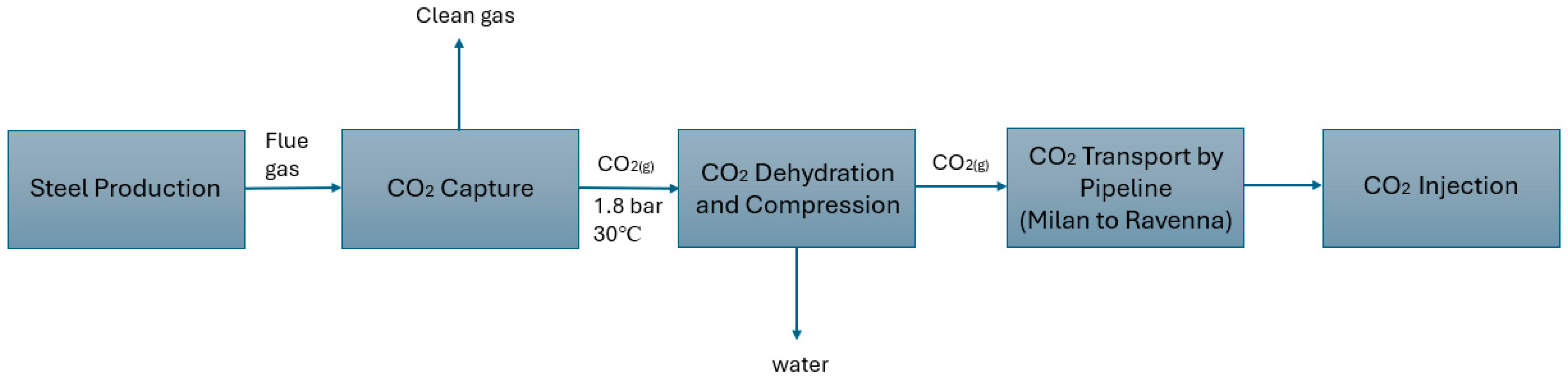
This process is simulated by using the Aspen Plus^® software (Bedford, MA 01730, USA) for representing the absorber+regeneration system. Furthermore, a techno-economic evaluation was integrated to enable an assessment of the economic feasibility of achieving high-capture performance in the steel plant applications and in storage in a saline aquifer, according to the block flow scheme reported in Figure 1.

2. Materials and Methods

2.1. Process Scheme

The design of the CO₂ capture process was carried out using Aspen Plus^® V11 as the simulation environment to model an absorption-regeneration system using a 30 wt.% aqueous monoethanolamine (MEA) solution to treat a blast furnace gas (BFG) stream from an integrated steel plant that could be incorporated with CCUS technology. The captured CO₂ is assumed to be transported to a geological storage site in the Adriatic Sea near Ravenna, where a national-scale carbon-capture and storage (CCS) hub is under development [17]. As the industrial facility under consideration is assumed to be located within the Milan metropolitan area, CO₂ is already present at the urban node of the regional transport network, eliminating the need for intermediate transport modes such as rail. The entire transfer from the steel plant to the injection site is therefore carried out via a dedicated long-distance pipeline, estimated to span approximately 300 km. This configuration constitutes a realistic infrastructure pathway for emitters in Lombardy, the highest industrialized region in Italy, given the absence of suitable local storage formations and the consequent necessity for cross-regional CO₂ transport.

The gaseous stream to be treated is characterized by a flow rate equal to 740.08 t/h, T = 305.15 K, P = 1.05 bar, composition = 21.59 mol% CO₂, 46.51 mol% N₂, 4.2 mol% H₂O [18], and with no MEA in that feed stream.

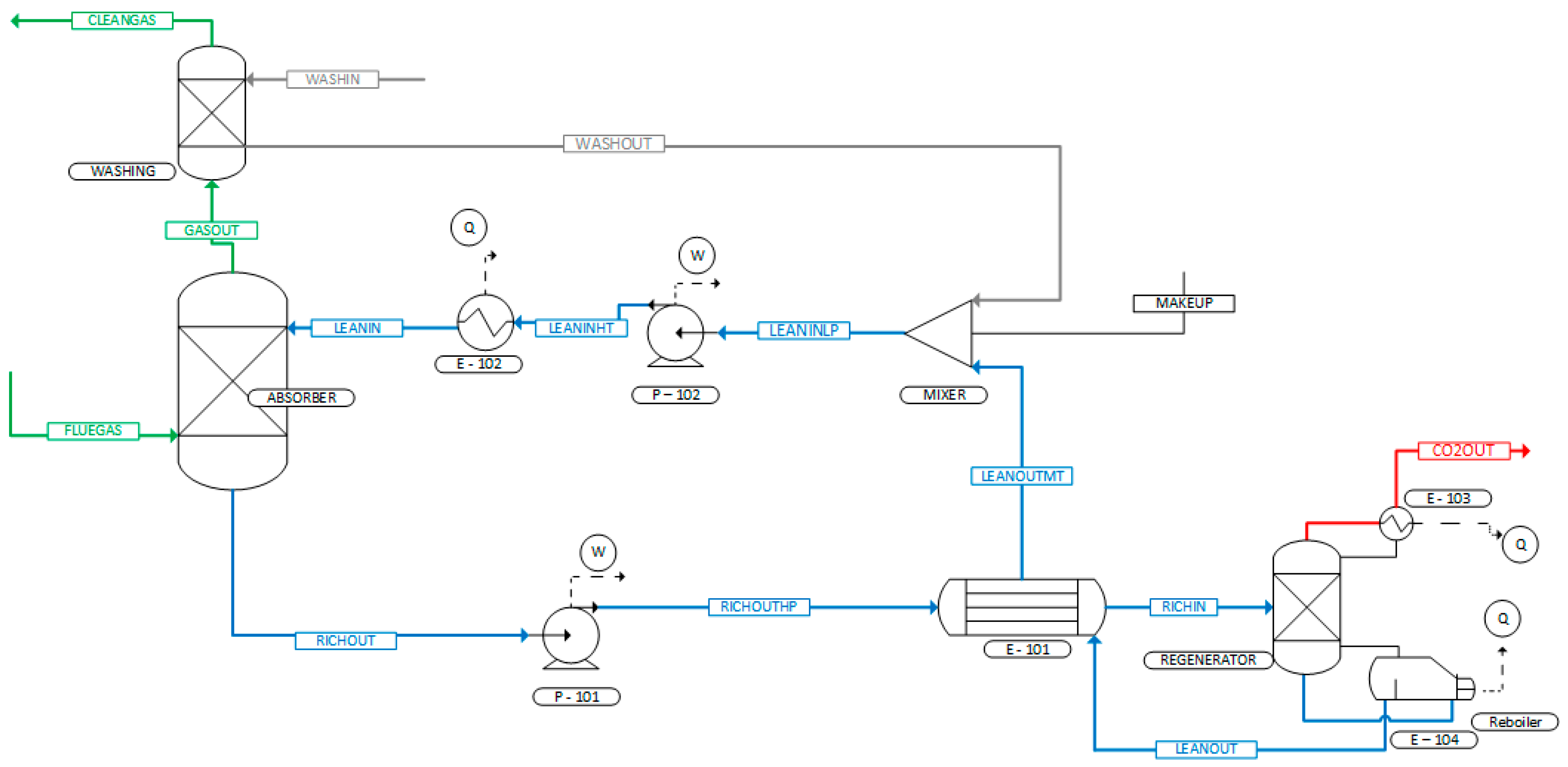
The ENRTL-RK model was selected as a thermodynamic property for the MEA-CO₂-H₂O system, where the Electrolyte- Non-Random Two-Liquid (NRTL) model [19,20,21,22] represented the non-ideal liquid phase behavior arising from chemical reactions and including the presence of charged species (H₃O⁺, OH⁻, CO₃⁻², MEACOO⁻, MEAH⁺, and HCO₃⁻), and the Perturbed-Chain Statistical Associating Fluid Theory (PC-SAFT) equation of state [23,24,25,26,27,28] was employed to model the vapor phase with improved accuracy for the systems containing polar compounds, as well as giving a realistic picture of how chain hydrocarbon molecules behave in a solution. The ENRTL–RK combined with PC-SAFT formulation has been applied and validated for reactive amine-based CO₂ capture systems as indicated by AspenTech™, offering a reliable description of vapor–liquid equilibrium, speciation, and thermophysical properties over a wide range of operating conditions. Figure 2 illustrates the process flow diagram of a steel plant for an MEA-based capture system to achieve 95% CO₂ removal. Both the absorber and the regenerator were modeled as rate-based units, with the integration of thermodynamics, chemical kinetics, and the transport phenomena, which all represent the system in a close approximation to reality. Other equipment, including a process–process heat exchanger, condenser, pumps, and washing section, was incorporated into the system for thermal integration and to minimize the MEA loss through evaporation.

The base case was adopted from the work of Schiattarella and Moioli [28]; however, the total flow rate of the lean solvent was adjusted to achieve the target CO₂ removal level, serving as the starting point for the designing the optimized process for 95% CO₂ removal. This process begins with the chemical absorption of the CO₂ in the BFG stream by the lean MEA solution introduced at the top of the absorber counter, currently resulting in a rich solvent stream. The rich solvent stream is then pumped to a heat exchanger to raise its temperature and facilitate the desorption process. The regenerated lean solvent stream is then cooled and recycled back to the absorber, while the main CO₂ product stream is obtained from the top through a thermal decomposition reaction driven by the reboiler heat duty in the regeneration column.

A water-wash section is installed at the top of the absorber to minimize the solvent losses and prevent amine carryover into the cleaned gas. This wash section is designed as a packed column in which the demineralized water is used to capture the entrained MEA droplets and ensure the treated flue gas meets the environmental discharge limits while maintaining the overall solvent economy by maximizing the solvent recovery, thereby reducing the solvent makeup cost.

In the present simulation, the washing water is introduced at a temperature of 298.15 K and with a pure-water composition, consistent with common industrial practice for amine-based CO₂ capture systems.

2.2. Parameter Selection and Optimization Approach

The optimization process aimed to determine the operating and design conditions that achieve the required 95% CO₂ capture efficiency while minimizing the total energy required for the regeneration process.

The first stage of this process focused on the absorber, as its dimensions and operating conditions strongly influence CO₂ capture efficiency, solvent circulation rate, and overall energy consumption.

Seven absorber heights were tested (10, 12, 16, 18, 20, and 22 m), each simulated across a range of lean loadings between 0.11 and 0.27 mol CO₂/mol MEA, in detail:

• from 0.11 to 0.23 [mol CO₂/mol MEA] for packing heights of 22 and 20 [m]
• from 0.11 to 0.21 [mol CO₂/mol MEA] for packing heights of 18 and 16 [m]
• from 0.11 to 0.17 [mol CO₂/mol MEA] for a packing height of 12 [m]
• for only 0.11 [mol CO₂/mol MEA] for a packing height of 10 [m].

The 14 m was skipped because the simulation was conducted by considering 10, 16, and 22 m, which means every 6 m of height, then focused on 18 and 20 m to better define the optimal one, but 12 m was only for better understanding the results at shorter heights.

The column diameter was determined for each absorber height and operating conditions based on hydraulic constraints, considering gas and liquid flow rates, packing characteristics, and flooding limits. For this reason, the diameter was not treated as an independent optimization variable but rather as an internally consistent design outcome of the rate-based model.

Once the optimal absorber packing height and lean loading were adjusted, the second stage targeted the regenerator since it is the major energy consumer in the process. The regenerator packing height varied from 6 to 20 m, and the optimal height was determined by balancing the stripper performance and energy consumption.

After that, the regenerator operating pressure was adjusted over the range of 0.6 to 2.5 bar, since regenerator pressure affects the equilibrium temperature and the CO₂ partial pressure, ending by varying the lean solvent inlet temperature from 30 to 50 °C.

2.3. Cost Estimation

2.3.1. CO₂ Removal

The economic evaluation quantifies how optimized operating conditions affect the capital and operating costs of the MEA-based CO₂ capture process. The methodology is based on recent CCUS techno-economic studies of Moioli et al. [14] related to the application of a CCS or a CCU section in a WtE plant, with adaptations reflecting the characteristics of an integrated steel plant in Lombardy.

The cost estimation considered 7900 annual operating hours, and all costs are expressed in US dollars. This assessment included all the major units in this process: absorber, regeneration column, condenser, reboiler, process–process heat exchanger, lean–rich heat exchanger, and pumps, and these units were dimensioned using the optimized simulation outputs.

The capital cost estimation was performed according to the method of Guthrie (1974), Ulrich (1984), and Navarrete (1995), which includes the purchased cost and bare module equipment cost.

The purchased cost of a given piece of equipment is calculated based on the previously purchased cost of the same unit, as expressed in Equation (1). The cost of each equipment item was updated using the Chemical Engineering Plant Cost Index (CEPCI).

$$C_2=C_1 \left({\displaystyle \frac{{Index}_2}{{Index}_1}}\right)$$

(1)

where $C_1$ is the known equipment cost at the reference year, $C_2$ is the adjusted cost for the concerned year, and ${Index}_1$ and ${Index}_2$ are the cost indices associated with the respective years. By applying the most recent available CEPCI values at the time of the assessment (June 2024), the equipment cost is updated for the current economic evaluation.

While the Bare Module Cost represents the sum of direct and indirect costs [29] to convert the basic purchase cost of the equipment into a more realistic estimate:

$$C_{BM}= C_P^0{F}_{BM}= C_P^0 (B_1+ B_2{F}_P{F}_M)$$

(2)

where $C_P^0$ is the purchased cost for base conditions, equipment made of the most common material (carbon steel), and operating at near-ambient pressures, $F_{BM}$ is the bare module cost factor, $F_P$ is the pressure factor, $F_M$ is the material factor, and $B_1$ and $B_2$ are coefficients associated with the specific equipment category.

Given the corrosive nature of amine solvents and the fact that the stripper and associated equipment operate at pressures above atmospheric, stainless steel is typically used as the material of construction. Its high resistance to chemical attack and its ability to withstand elevated pressures ensure the reliable and safe operation of CO₂ capture units.

The costs of the purchased equipment were estimated using the following formula:

$${log}_{10}\left(C_P^0\right)= K_1+K_2{log}_{10}\left(A\right)+K_3{\left[{log}_{10}\left(A\right)\right]}^2$$

(3)

where $A$ is the relevant size parameter (e.g., area, volume), and $K_1$, $K_2$, and $K_3$ are correlation constants specified for each equipment type and the economic evaluation year.

To apply these correlations, the necessary cost constants, material factors, and pressure-correction parameters are reported in

Table 1. Constants for bare module and material factors.

Equipment Type	Equipment Description	B1	B2	Construction Material	FM
Absorption Tower		2.25	1.82	SS	3.10
Regeneration Tower		2.25	1.82	SS	3.10
Condenser	Floating Head	1.63	1.66	SS	2.70
Reboiler	Kettle Reboiler	1.63	1.66	SS	2.70
E-102	Flat Plate	0.96	1.21	SS	2.70
E-103	Flat Plate	0.96	1.21	SS	2.70
P-101	Centrifugal	1.89	1.35	SS	2.30
P-102	Centrifugal	1.89	1.35	SS	2.30

,

Table 2. Constants for purchased cost [14].

Equipment Type	K1	K2	K3
Absorption Tower	3.4974	0.4485	0.1074
Absorber Packing	2.4493	0.9744	0.0055
Regeneration Tower	3.4974	0.4485	0.1074
Regenerator Packing	2.4493	0.9744	0.0055
Condenser	4.8306	−0.8509	0.3187
Reboiler	4.4646	−0.5277	0.3955
E-102	4.6656	−0.1557	0.1547
E-103	4.6656	−0.1557	0.1547
P-101	3.3892	0.0536	0.1538
P-102	3.3892	0.0536	0.1538

and

Table 3. Pressure factors [14].

Equipment Type	Equipment Description	C1	C2	C3	P [barg]
Reboiler	Kettle Reboiler	0.03881	−0.11272	0.08183	4.49

corresponding to the equipment classes relevant to this CO₂ capture process. These values allow direct computation of the purchased cost, bare module cost, and the overall total module cost.

The total module cost (C_TM) was determined by adding a 15% contingency allowance to the sum of all bare module costs. Additionally, a further 3% of C_TM was included to cover permitting and authorization expenses, which include environmental evaluations and regulatory approvals necessary for the installation of a CO₂ capture system at this industrial steel facility in Lombardy.

Operating costs (cost of manufacturing, COM) include labor, utilities, and raw materials costs, and these were calculated according to the procedure adapted from Turton et al. [29], with adjustments introduced to reflect the specific operating conditions and utility costs typical of steelmaking plants in the Milan region. The cost of the solvent was 6.02 $/L [30] while the demi-water was based on the value of Moioli et al. [31].

2.3.2. CO₂ Sequestration in Saline Aquifer

To estimate the economic impact of the downstream stages illustrated in Figure 2, this study utilizes the cost correlations and methodological framework established by Stolaroff et al. [32] for dehydration and compression, for transport by pipelines and for sequestration in saline aquifers.

The literature provides reference values for CO₂ transport under various conditions. For instance, Geo et al. [33] reported transport costs of approximately 13 $/tCO₂ for a long-distance (600 km) rail scenario, including additional charges for loading operations. Roussanaly et al. [15] identified transport costs ranging from 4 to 11 €/tCO₂ for pipeline routes between 50 and 200 km, with about 1 €/tCO₂ attributed to terminal handling. Building on these analyses, Stolaroff et al. [32] included an additional 2 $/tCO₂ to account for the rail transport cost. Reported upper-bound values for extended pipeline corridors reach approximately 24 $/tCO₂.

2.4. Business Plan

A techno-economic business plan was developed to assess the financial feasibility of installing a post-combustion MEA-based CO₂ capture unit at the Lombardy steel plant, along with geologic injection of the captured CO₂ into the Ravenna saline aquifer.

The business analysis combines capital expenditure (CAPEX) and operational expenditure (OPEX) from Section 2.3 to evaluate overall project profitability under selected policy and market assumptions.

Economic performance is assessed using net present value (NPV), calculated with a weighted average cost of capital (WACC) consistent with recent industrial energy investment analyses. A WACC of 8.3% is assumed, following the methodology already applied in other Italian industrial decarbonization studies [34].

The calculation model includes the following annual cost and revenue components:

• investment cost of the capture plant, distributed over the project lifetime
• operating costs of the CO₂ capture plant
• mass flow rate of CO₂ removed from the BF gas
• electricity consumption of the CO₂ capture and compression systems, based on the average industrial power cost in Northern Italy
• transport and injection cost of CO₂ into the Ravenna saline aquifer
• the value (or absence) of the EU ETS carbon price, depending on the scenario considered.

For geological storage, the economic impact of CO₂ sequestration was considered a negative overall revenue. This cost was estimated using the literature values for CO₂ injection into saline aquifers, as detailed in Section 2.3.1.

Accordingly, the total annual revenues of the project were defined as the sum of two main contributions:

i.

The economic balance associated with CO₂ sequestration, which is negative due to transport and injection costs.

ii.

The financial benefit arising from avoided CO₂ emissions through the allocation of EU ETS certificates. That term is inherently positive, as it reflects the reduction in CO₂ emissions released into the atmosphere.

The financial assessment was carried out considering the applicable Italian fiscal framework for industrial facilities located in Lombardy. In particular, the Regional Tax on Productive Activities (Imposta Regionale sulle Attività Produttive, IRAP), equal to 3.9%, and the Corporate Income Tax (Imposta sui Redditi delle Società, IRES), equal to 24%, were applied consistently across all scenarios.

The business plan model calculates the main economic indicators required to evaluate project profitability, including the NPV, while accounting for inflation effects, operating costs, and the impact of ETS-related revenues associated with avoided CO₂ emissions. A range of ETS carbon price levels was considered, spanning from 20 to 100 USD per tonne of CO₂, with values escalated annually according to the assumed inflation rate. In scenarios where the CO₂ sequestration option resulted in a negative NPV, the corresponding breakeven carbon price was also determined in order to identify the minimum ETS value required to achieve economic viability.

To explore the influence of policy conditions on project feasibility, the following scenarios were examined:

• Carbon tax (ETS price applied), without CO₂ storage.
• Absence of carbon tax (ETS price equal to zero), without CO₂ storage.
• Carbon tax applied, with CO₂ transported via pipeline and injected into the Ravenna storage site.
• Absence of carbon tax, with CO₂ injection into the Ravenna saline aquifer.

The influence of inflation was also considered.

This combined scenario-based and sensitivity-based assessment provides a comprehensive view of the potential financial outcomes of integrating CO₂ capture and geological storage at a steel plant under both favorable and constrained policy conditions.

3. Results

3.1. Process Optimization

3.1.1. Optimization of the Absorber Height and Lean Loading

The optimization was conducted following a sequential approach based on process sensitivity and physical relevance. The absorber height was optimized first together with the lean loading, as it directly determines the extent of gas–liquid contact, and they largely determine the achievable CO₂ capture efficiency for a given solvent circulation rate.

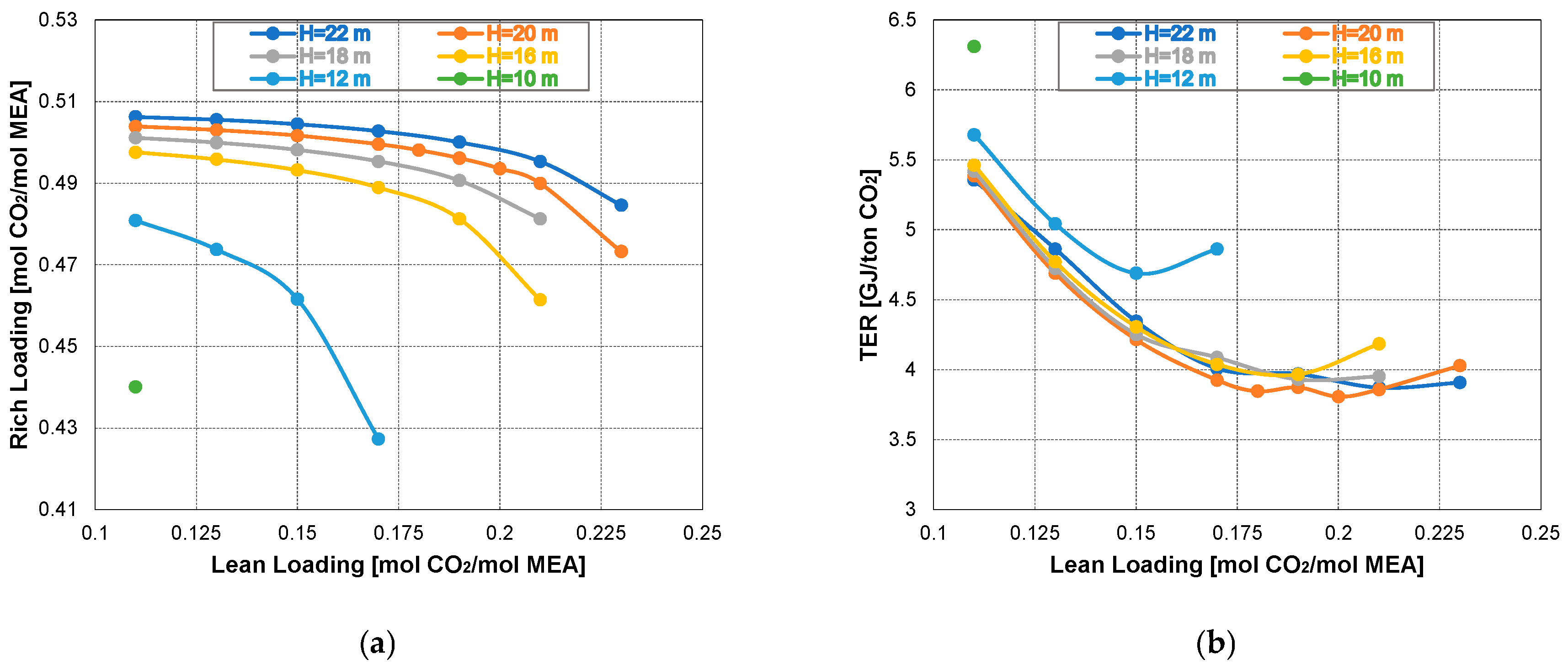
Figure 3a illustrates how the rich loading varies as a function of lean loading of MEA for different absorber heights. The results highlight the critical role of the column height in determining the CO₂ absorption capacity. For taller absorbers (20–22 m), rich loading values consistently remained above 0.50 mol CO₂/mol MEA, which indicates that these configurations provide sufficient contact area and residence time for effective CO₂ transfer from the gas phase to the solvent. By contrast, shorter absorbers (10–12 m) exhibited significantly reduced performance, which is restricted to the insufficient height of the column and contact area.

The thermal energy requirement (TER) is the major indicator for the reboiler duty performance. All curves exhibit a characteristic U-shaped profile, in which TER decreased at higher lean loading from (0.10–0.20 mol CO₂/mol MEA). The minimum TER values, around 3.8–4 GJ/ton CO₂, are achieved at taller absorber heights of 20–22 m, ensuring that taller columns promote more efficient CO₂ mass transfer and richer solvent loading, thereby lowering the specific reboiler duty. These TER obtained values are consistent with values reported in the literature for CO₂ capture from blast furnace gas (BFG), which depends on the process configuration, capture rate, and integration with water-gas shift units or heat recovery systems [17,35].

Beyond a lean loading of 0.20 mol CO₂/mol MEA, the TER starts to increase again across all the absorber heights. This is attributed to reduced absorption efficiency at high lean loading, which forces higher solvent circulation rates and increased regeneration energy to achieve the same CO₂ capture target.

Overall, from these analyses, the optimal values for both the lean loading and the absorber packing heights can be set as α = 0.20 mol CO₂/mol MEA and H_abs = 20 m, while the obtained TER is equal to 3.8 GJ/ton CO₂. These values are different from the optimal values obtained for 90% CO₂ removal by Schiattarella and Moioli [28], confirming that each process must be designed for the specific target of CO₂ to be removed to optimize its performance.

3.1.2. Optimization of the Regenerator Height

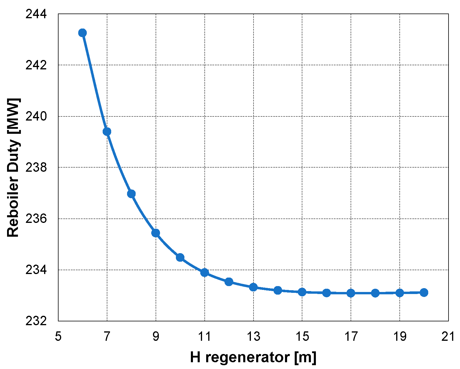
The regenerator represents the dominant contributor to the overall energy penalty and determines the quantity of the regenerated lean solvent. Since the reboiler duty accounts for the majority of the process steam demand, Figure 4 illustrates the effect of varying the regenerator packing height with its duty. The results reveal a steep decreasing trend in reboiler energy consumption as the regenerator height increases from 6 to 12 m. Specifically, at very short heights (6–9 m), the reboiler duty is significantly higher, which can be attributed to the limited packing area that reduces the effective contact between the rising vapor and descending solvent, leading to a decrease in the stripping efficiency as well as requiring a larger amount of steam in the reboiler to achieve the same level of CO₂ desorption. Beyond approximately 14 m, the curve progressively flattens, suggesting that further increases in packing height yield diminishing returns. The height of 15 m was selected as the optimal value, as the reboiler duty has nearly reached its minimum, while any further increase would require higher capital investment due to additional column materials, installation costs, and potentially larger footprints, without delivering proportional energy savings.

3.1.3. Optimization of the Regenerator Pressure

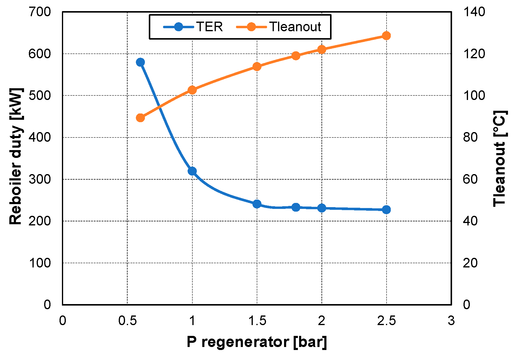
After identifying the absorber height, lean loading, and regenerator height optimal values, the regenerator pressure must be investigated, as it determines the equilibrium temperature of the stripper and the driving force for CO₂ release. As shown in Figure 5, the regenerator pressure varied from 0.6 to 2.5 bar while monitoring the thermal energy requirement and the lean solvent outlet temperature.

On the right-hand Y-axis, the lean solvent outlet temperature rises steadily with the pressure to nearly 130 °C at 2.5 bar; this behavior reflects the increase in the boiling temperature of the solvent mixture. These higher temperatures can improve stripping efficiency, but they also risk MEA thermal degradation above ~120 °C [36]. This issue has been studied in the literature. The conventional stripper temperature is considered to be 120 °C, as reported in Braakhuis et al. [37], who studied the formation of the degradation compounds during the thermal degradation of the MEA solvent.

On the left-hand Y-axis, TER is extremely high at very low pressure, then declines steeply as the stripper pressure increases, allowing the CO₂ partial pressure rise and leading to the easier release of the gas from the solvent.

Taking both trends into account, the optimal pressure of 1.8 bar was chosen in order to have a minimum TER while maintaining the lean-out temperature below the critical degradation threshold.

3.1.4. Optimization of the Lean Solvent Inlet Temperature

The influence of lean solvent inlet temperature on CO₂ absorber performance was assessed by varying the temperature from 30 to 50 °C. The results indicate that inlet temperature exerts only a minor effect on the system’s overall energy requirement. An inlet temperature of 35 °C was selected, as it provides a modest improvement in regeneration duty without incurring operational penalties.

3.1.5. Comparison with the Previous Literature

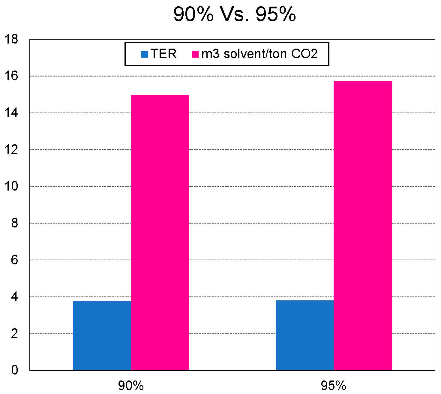
Figure 6 and

Table 4. TER and solvent flow rate comparison of the considered cases.

	90% CO2 Removal	95% CO2 Removal
TER [GJ/tCO2]	3.75	3.78
Solvent flow rate [m3/tCO2]	14.96	16

present a comparison of the thermal energy requirement (TER) and the specific lean solvent circulation rate for the optimized 90% and 95% CO₂ capture scenarios. Increasing the capture efficiency from 90% to 95% results in a marginal increase in TER, from 3.75 to 3.78 GJ per ton of CO₂, demonstrating that higher capture efficiencies can be achieved without a significant energy penalty when the process is optimized.

However, increasing the capture efficiency results in a higher specific solvent circulation rate, rising from approximately 15.0 to 16.0 m³ of solvent per ton of CO₂ captured. This outcome aligns with solvent-based absorption theory, which states that deeper CO₂ removal requires higher solvent circulation to compensate for the reduced mass-transfer driving force at low CO₂ partial pressures.

When compared with previous MEA-based CO₂ capture studies applied to industrial systems, such as the work of Schiattarella et al. [28], which focused on a 90% capture target, the present results demonstrate that a 95% capture efficiency can be reached while maintaining a comparable energy demand. This highlights the effectiveness of the proposed optimization strategy and confirms that MEA-based capture remains a technically viable option even at higher removal efficiencies. The corresponding optimized operating parameters for the 95% capture efficiency are reported in

Table 5. Optimized parameters for the 95% CO₂ removal section.

Parameter	Unit	Optimized Value
Absorber packed height	[m]	20
Lean loading	[-]	0.20
Regenerator packed height	[m]	15
Regenerator pressure	[bar]	1.8
Lean solvent temperature	[°C]	35
TER	[GJ/ton CO2]	3.78

.

3.1.6. Mass Reflux Ratio Behavior in the Regenerator

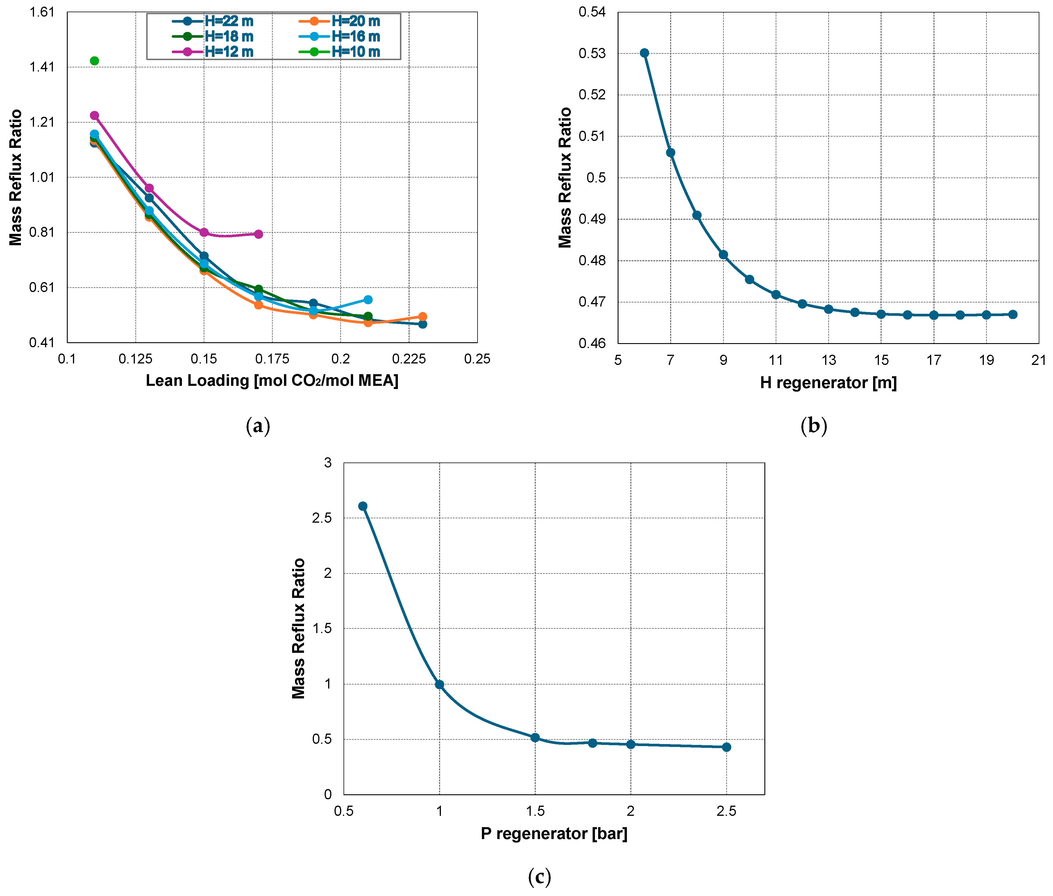
The mass reflux ratio was examined to analyze the regenerator’s behavior under varying operating conditions, as it quantifies the liquid reflux returning from the condenser relative to the vapor flow produced in the reboiler.

Although the mass reflux ratio (MRR) is calculated in the regenerator, it is influenced by the CO₂ loading in the rich solvent exiting from the absorber.

From the absorber optimization results, it was observed that shorter columns limit mass transfer efficiency, leading to lower rich loading and higher internal reflux.

In contrast, taller columns, specifically the optimal height of 20 m at 0.2 mol CO₂/mol MEA, produce a moderate rich loading, and the regenerator operates at a low reflux ratio, which confirms the suitability of this operating point for minimizing the energy demand.

Figure 7b shows that by increasing the regenerator height, the MRR reduces, leading to a reduction of the circulation requirements beyond 15 m; the MRR shows a constant trend.

This trend confirms that a 15 m height represents an energetically favorable and hydraulically stable design point, providing adequate stripping capacity without unnecessary capital cost. The complete material balance of the optimized 95% CO₂ removal process, including stream temperature, pressure, and compositions, is presented in

Table 6. Material balance of the optimized scheme for 95% CO₂ removal.

Stream	FLUE GAS	WASH IN	CLEAN GAS	MAKE UP	CO2 OUT
T [K]	308.15	298.15	338.79	298.15	303.15
P [bar]	1.05	1.20	1.00	1.01325	1.8
Mass flow [t/h]	740.0777	27.1336	616.172	0.0019	224.175
Mole flow [Kmol/h]	24,569.8	1506.14	24,971.4	3.13
Mole fraction [%mol]					5169.25
MEA	0	0	1.254 × 10−4	100	6.71 × 10−9
H2O	4.20	100	25.96	0	2.39
CO2	21.59	0	1.04	0	97.48
N2	46.51	0	45.78	0	0.06
O2	0.60	0	0.59	0	1.553 × 10−3
CO	23.45	0	23.06	0	0.04
H2	3.65	0	3.59	0	7.43 × 10−3

.

Figure 7c shows that the optimal regenerator pressure provides the trade-off between low MRR and efficient CO₂ desorption.

3.2. Economic Evaluation

The economic evaluation was carried out using the same methodology as Schiattarella and Moioli [28]. However, in the present work, the cost parameters were updated to reflect current economic conditions. All equipment costs were calculated using CEPCI values of 798.8 for June 2024, while the reference CEPCI values were 394.3 for the year 2001 and 584.6 for the year 2012 [38].

Table 7. Bare module cost for the optimized process for 90% CO₂ capture.

Equipment Type	Capacity	Unit Number	${\mathit{C}}_{\mathit{P}}^0$ of a Single Unit [$]	${\mathit{C}}_{\mathit{P}}^0$ [$]
Absorption Tower	3023.09 [m3]	1	1,875,263.83	1,875,263.83
Absorber Packing	2015.39 [m3]			674,746.43
Regeneration Tower	731.21 [m3]	1	800,230.90	800,230.90
Regenerator Packing	461.81 [m3]			246,158.45
Condenser	2432.42 [m2]	2	319,019.03	638,038.06
Reboiler	5172.03 [m2]	3	1,095,809.79	3,287,429.37
E-102	70,100.46 [m2]	34	1,218,867.41	41,441,492.10
E-103	3288.04 [m2]	2	1,064,034.03	2,128,068.06
P-101	206.81 [kW]	1	43,813.84	43,813.84
P-102	88.10 [kW]	1	23,927.50	23,927.50

,

Table 8. Bare module cost for the optimized process for 95% CO₂ capture.

Equipment Type	Capacity	Unit Number	${\mathit{C}}_{\mathit{P}}^0$ of a Single Unit [$]	${\mathit{C}}_{\mathit{P}}^0$ [$]
Absorption Tower	3386.91 [m3]	1	2,007,584.84	2,007,584.84
Absorber Packing	2322.45 [m3]			734,670.83
Regeneration Tower	1077.32 [m3]	1	1,009,714.07	1,009,714.07
Regenerator Packing	673.32 [m3]			349,509.82
Condenser	2557.77 [m2]	2	328,783.97	657,567.95
Reboiler	5172.03 [m2]	3	1,137,503.75	3,412,511.25
E-102	76,253.69 [m2]	37	1,218,559.61	45,086,705.47
E-103	3947.40 [m2]	2	1,187,353.18	2,374,706.35
P-101	231.28 [kW]	1	47,773.12	47,773.12
P-102	97.97 [kW]	1	25,663.32	25,663.32

,

Table 9. Operating labor cost for the optimized process for 90% and 95% CO₂ removal.

Operating Labor, COL	Unit	Value
		90% CO2 Capture	95% CO2 Capture
Total Equipment for Handling Fluids	[-]	43	46
Total Equipment for Handling Solids	[-]	0	0
Number of Operators for One Shift	[op/shift]	5	5
Plant Operability	[h/y]	7900	7900
Time for Shift	[h/shift]	8	8
Weekly Shifts	[shift/week]	5	5
Working Weeks	[weeks/y]	48	48
Shifts for the Year Required in a Plant (tot)	[shift/y]	987.5	987.5
Yearly Shifts of Each Operator	[shift/y]	240	240
Rounded Number of Required Operators for the Same Unit at Different Times	[n/y unit]	5	5
Total Number of Required Operators for the Plant	[n/y unit]	25	25
Average Yearly Operator Wage	[€/y]	40,000	40,000
$ Value	[$/€]	0.8641	0.8641
Average Yearly Operator Wage	[$/y]	34,564	34,564

,

Table 10. Utility expenses for 90% CO₂ capture.

Utility Type	Cost [$/GJ]	Used [GJ/y]	Total Cost [M$/y]
Electrical substation	16.8	8386.98	1.41 × 10−1
Steam from boilers, low pressure (5 barg, 160 °C)	14.05	6,230,200.81	87.53
Cooling tower water (30 °C to 40–45 °C)	0.354	3,953,725.64	1.40
Total			89.0748
Total (adjusted with CEPCI 06/2024)			121.7123

,

Table 11. Utility expenses for 95% CO₂ capture.

Utility Type	Cost [$/GJ]	Used [GJ/y]	Total Cost [M$/y]
Electrical substation	16.8	9364.11	1.57 × 10−1
Steam from boilers, low pressure (5 barg, 160 °C)	14.05	6,630,274.08	93.16
Cooling tower water (30 °C to 40–45 °C)	0.354	4,524,794.94	1.60
Total			94.9144
Total (adjusted with CEPCI 06/2024)			129.6915

,

Table 12. Raw material cost for 90% CO₂ capture.

Raw Material Type	Cost	Used Per Year	Cost [M$/y]
Demi water	0.0018 [$/kL]	642,510.30 [kl/y]	1.16 × 10−3
Amine make-up (for losses due to volatility)	5.95 [$/kg]	15,743.32 [kg/y]	9.37 × 10−2
Amine make-up (for degradation)	5.95 [$/kg]	1927.09 [t/y]	11.47
Total			11.5603

,

Table 13. Raw material cost for 95% CO₂ capture.

Raw Material Type	Cost	Used Per Year	Cost [M$/y]
Demi water	0.0018 [$/kL]	579,002.27 [kl/y]	1.04 × 10−3
Amine make-up (for losses due to volatility)	5.95 [$/kg]	15,112.36 [kg/y]	8.99 × 10−2
Amine make-up (for degradation)	5.95 [$/kg]	2032.41 [t/y]	12.09
Total			12.1830

,

Table 14. Initial solvent cost.

Type of Expenses	Unit	Value
		90% CO2 Capture	95% CO2 Capture
Initial fill circulating solvent	[kg]	2,468,952.50	2,746,625.00
Amine unit cost	[$/L]	6.02	6.02
Water unit cost	[$/kg]	0.0018	0.0018
Solvent unit cost	[$/kg]	1.7861	1.7861
Cost for solvent	[$]	4,409,898.33	4,905,860.69
Cost for corrosion inhibitor	[$]	5,291,878	5,887,033
Number of trucks	[-]	124	138

and

Table 15. Total plant cost.

Plant Total Cost	Unit	Value
		90% CO2 Capture	95% CO2 Capture
Plant life	[y]	25	25
Fixed capital investment (FCI)	[M$]	419.28	460.73
Fixed capital investment	[M$/y]	16.77	18.43
Cost of manufacturing (COM)	[M$/y]	178.32	190.80
Total cost during the entire period	[M$/y]	195.09	209.23
Cost of removed CO2	[$/tCO2]	117.44	119.42
FCI per ton of removed CO2	[$/tCO2]	10.10	10.52
COM per ton of removed CO2	[$/tCO2]	107.34	108.90

present the economic analysis results for both scenarios, detailing the bare module cost, operating labor cost, utility, and raw materials expenses, ending with the total cost for both plants.

The amine make-up cost for degradation in Table 12 (12.09 M$/y) is significantly higher than that for volatility (0.089 M$/y), highlighting the critical role of temperature control in MEA-based CO₂ capture systems. In this study, a regenerator pressure of 1.8 bar was chosen to maintain the lean solvent outlet temperature below the thresholds for accelerating the MEA degradation. Therefore, the selected pressure–temperature operating point represents a compromise between minimizing energy consumption and limiting solvent degradation, supporting both economic viability and long-term operational stability of the capture system.

The fixed capital investment (FCI) increased from 419.28 M$ to 460.73 M$, reflecting the additional required capacity for both absorber and regenerator to achieve higher removal efficiency as well as the total number of operated units. By considering 25 years, the FCI per year can be estimated to be equal to 18.43 M$/y.

Similarly, the annual cost of manufacturing (COM) increased from 178.32 M$/y to 190.80 M$/y due to the steam demand for regenerating the solvent at a higher capacity. The cost of removed CO₂ increased slightly from 117.44 $/tCO₂ to 119.42 $/tCO_2, as expected, because the higher CO₂ removal makes the process more difficult as a result of the low driving force for CO₂ absorption at the top of the absorption column, while the FCI per ton of removed CO₂ has a slight difference in both cases.

Most of this cost is related to COM, which shifts from 107.34 $/tCO₂ to 108.90 $/tCO₂, indicating that even though the higher removal efficiency requires an additional investment and energy consumption, the cost per ton of CO₂ removed remains modest, demonstrating the economic feasibility of moving from 90% to 95% CO₂ capture in large-scale steel plant applications.

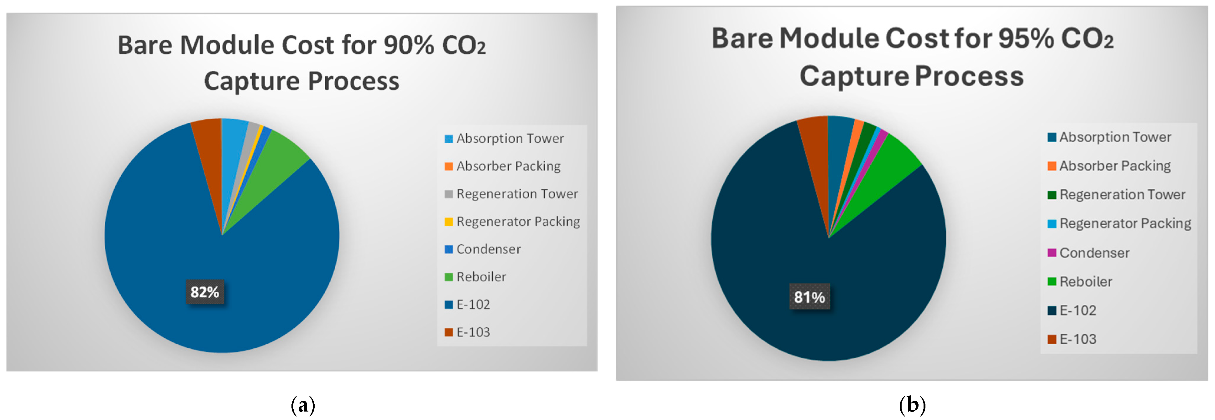
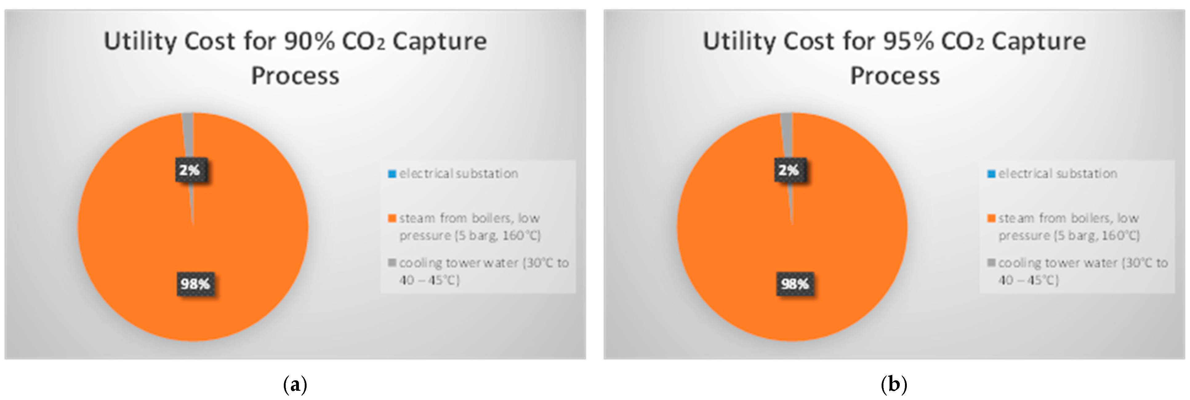
Figure 8 illustrates the bare module cost for the 90% and 95% CO₂ removal to better clarify the key economic parameters, while Figure 9 shows the utility cost for both scenarios, and the fact that the low-pressure steam required for solvent regeneration dominated the utility costs, while electricity and cooling water contributions remain marginal with a similar overall cost structure.

Cash Flow Analysis

The economic performance of the optimized CO₂ capture system was assessed by developing a multi-year cash-flow model for the steel plant. Two financial scenarios were evaluated:

• Base case without inflation.
• Scenario including annual inflation of operating expenses and revenues.

Carbon tax effects were not included at this stage, but an indicative carbon tax value corresponding to the breakeven NPV (NPV = 0) was estimated to identify the minimum carbon price required to make the project economically neutral.

The resulting cash-flow tables for all years of operation are reported below in

Table 16. Cash flow of the CO₂ capture process without inflation, carbon tax not considered, and with an injection in a saline aquifer for 90% CO₂ removal (E+ = ×10^).

Year	2024	2025		2026	2027	2028	2029	2030	2031		2032
Years of operation	0	1		2	3	4	5	6	7		8
Year of discounting	1	2		3	4	5	6	7	8		9
Revenues	0	−1.39E+08		−1.39E+08	−1.39E+08	−1.39E+08	−1.39E+08	−1.39E+08	−1.39E+08		−1.39E+08
CAPEX of CO2 capture	3.46E+08	0		0	0	0	0	0	0		0
OPEX of CO2 capture	0	1.78E+08		1.78E+08	1.78E+08	1.78E+08	1.78E+08	1.78E+08	1.78E+08		1.78E+08
EBITDA	0	−3.18E+08		−3.18E+08	−3.18E+08	−3.18E+08	−3.18E+08	−3.18E+08	−3.18E+08		−3.18E+08
Depreciation	0	2.13E+07		2.13E+07	2.13E+07	2.13E+07	2.13E+07	2.13E+07	2.13E+07		2.13E+07
EBIT	0	−3.39E+08		−3.39E+08	−3.39E+08	−3.39E+08	−3.39E+08	−3.39E+08	−3.39E+08		−3.39E+08
IRAP	0	−1.32E+07		−1.32E+07	−1.32E+07	−1.32E+07	−1.32E+07	−1.32E+07	−1.32E+07		−1.32E+07
IRES	0	−8.14E+07		−8.14E+07	−8.14E+07	−8.14E+07	−8.14E+07	−8.14E+07	−8.14E+07		−8.14E+07
NOPAT	0	−2.44E+08		−2.44E+08	−2.44E+08	−2.44E+08	−2.44E+08	−2.44E+08	−2.44E+08		−2.44E+08
Cash from operations	0	−2.23E+08		−2.23E+08	−2.23E+08	−2.23E+08	−2.23E+08	−2.23E+08	−2.23E+08		−2.23E+08
Net Cash Flow	−3.46E+08	−2.23E+08		−2.23E+08	−2.23E+08	−2.23E+08	−2.23E+08	−2.23E+08	−2.23E+08		−2.23E+08
2033	2034	2035	2036	2037	2038	2039	2040	2041	2042	2043	2044
9	10	11	12	13	14	15	16	17	18	19	20
10	11	12	13	14	15	16	17	18	19	20	21
−1.39E+08	−1.39E+08	−1.39E+08	−1.39E+08	−1.39E+08	−1.39E+08	−1.39E+08	−1.39E+08	−1.39E+08	−1.39E+08	−1.39E+08	−1.39E+08
0	0	0	0	0	0	0	0	0	0	0	0
1.78E+08	1.78E+08	1.78E+08	1.78E+08	1.78E+08	1.78E+08	1.78E+08	1.78E+08	1.78E+08	1.78E+08	1.78E+08	1.78E+08
−3.18E+08	−3.18E+08	−3.18E+08	−3.18E+08	−3.18E+08	−3.18E+08	−3.18E+08	−3.18E+08	−3.18E+08	−3.18E+08	−3.18E+08	−3.18E+08
2.13E+07	2.13E+07	2.13E+07	2.13E+07	2.13E+07	2.13E+07	2.13E+07	8.51E+05	8.51E+05	8.51E+05	8.51E+05	8.51E+05
−3.39E+08	−3.39E+08	−3.39E+08	−3.39E+08	−3.39E+08	−3.39E+08	−3.39E+08	−3.19E+08	−3.19E+08	−3.19E+08	−3.19E+08	−3.19E+08
−1.32E+07	−1.32E+07	−1.32E+07	−1.32E+07	−1.32E+07	−1.32E+07	−1.32E+07	−1.24E+07	−1.24E+07	−1.24E+07	−1.24E+07	−1.24E+07
−8.14E+07	−8.14E+07	−8.14E+07	−8.14E+07	−8.14E+07	−8.14E+07	−8.14E+07	−7.64E+07	−7.64E+07	−7.64E+07	−7.64E+07	−7.64E+07
−2.44E+08	−2.44E+08	−2.44E+08	−2.44E+08	−2.44E+08	−2.44E+08	−2.44E+08	−2.30E+08	−2.30E+08	−2.30E+08	−2.30E+08	−2.30E+08
−2.23E+08	−2.23E+08	−2.23E+08	−2.23E+08	−2.23E+08	−2.23E+08	−2.23E+08	−2.29E+08	−2.29E+08	−2.29E+08	−2.29E+08	−2.29E+08
−2.23E+08	−2.23E+08	−2.23E+08	−2.23E+08	−2.23E+08	−2.23E+08	−2.23E+08	−2.29E+08	−2.29E+08	−2.29E+08	−2.29E+08	−2.29E+08

,

Table 17. Cash flow of the CO₂ capture process with inflation, carbon tax not considered, and with an injection in a saline aquifer for 90% CO₂ removal (E+ = ×10^).

Year	2024	2025	2026		2027	2028	2029	2030	2031		2032
Years of operation	0	1	2		3	4	5	6	7		8
Year of discounting	1	2	3		4	5	6	7	8		9
Revenues	0	−1.46E+08	−1.49E+08		−1.51E+08	−1.53E+08	−1.56E+08	−1.58E+08	−1.60E+08		−1.63E+08
CAPEX of CO2 capture	3.46E+08	0	0		0	0	0	0	0		0
OPEX of CO2 capture	0	1.87E+08	1.90E+08		1.93E+08	1.96E+08	1.99E+08	2.02E+08	2.05E+08		2.08E+08
EBITDA	0	−3.33E+08	−3.39E+08		−3.44E+08	−3.49E+08	−3.55E+08	−3.60E+08	−3.66E+08		−3.71E+08
Depreciation	0	2.13E+07	2.13E+07		2.13E+07	2.13E+07	2.13E+07	2.13E+07	2.13E+07		2.13E+07
EBIT	0	−3.55E+08	−3.60E+08		−3.65E+08	−3.71E+08	−3.76E+08	−3.82E+08	−3.87E+08		−3.92E+08
IRAP	0	−1.38E+07	−1.40E+07		−1.42E+07	−1.45E+07	−1.47E+07	−1.49E+07	−1.51E+07		−1.53E+07
IRES	0	−8.51E+07	−8.64E+07		−8.77E+07	−8.90E+07	−9.03E+07	−9.16E+07	−9.29E+07		−9.42E+07
NOPAT	0	−2.56E+08	−2.60E+08		−2.63E+08	−2.67E+08	−2.71E+08	−2.75E+08	−2.79E+08		−2.83E+08
Cash from operations	0	−2.34E+08	−2.38E+08		−2.42E+08	−2.46E+08	−2.50E+08	−2.54E+08	−2.58E+08		−2.62E+08
Net Cash Flow	−3.46E+08	−2.34E+08	−2.38E+08		−2.42E+08	−2.46E+08	−2.50E+08	−2.54E+08	−2.58E+08		−2.62E+08
2033	2034	2035	2036	2037	2038	2039	2040	2041	2042	2043	2044
9	10	11	12	13	14	15	16	17	18	19	20
10	11	12	13	14	15	16	17	18	19	20	21
−1.65E+08	−1.68E+08	−1.70E+08	−1.72E+08	−1.75E+08	−1.77E+08	−1.79E+08	−1.82E+08	−1.84E+08	−1.86E+08	−1.89E+08	−1.91E+08
0	0	0	0	0	0	0	0	0	0	0	0
2.11E+08	2.14E+08	2.17E+08	2.20E+08	2.23E+08	2.26E+08	2.30E+08	2.33E+08	2.36E+08	2.39E+08	2.42E+08	2.45E+08
−3.76E+08	−3.82E+08	−3.87E+08	−3.93E+08	−3.98E+08	−4.03E+08	−4.09E+08	−4.14E+08	−4.20E+08	−4.25E+08	−4.30E+08	−4.36E+08
2.13E+07	2.13E+07	2.13E+07	2.13E+07	2.13E+07	2.13E+07	2.13E+07	8.51E+05	8.51E+05	8.51E+05	8.51E+05	8.51E+05
−3.98E+08	−4.03E+08	−4.09E+08	−4.14E+08	−4.19E+08	−4.25E+08	−4.30E+08	−4.15E+08	−4.21E+08	−4.26E+08	−4.31E+08	−4.37E+08
−1.55E+07	−1.57E+07	−1.59E+07	−1.61E+07	−1.64E+07	−1.66E+07	−1.68E+07	−1.62E+07	−1.64E+07	−1.66E+07	−1.68E+07	−1.70E+07
−9.55E+07	−9.68E+07	−9.80E+07	−9.93E+07	−1.01E+08	−1.02E+08	−1.03E+08	−9.96E+07	−1.01E+08	−1.02E+08	−1.04E+08	−1.05E+08
−2.87E+08	−2.91E+08	−2.95E+08	−2.98E+08	−3.02E+08	−3.06E+08	−3.10E+08	−2.99E+08	−3.03E+08	−3.07E+08	−3.11E+08	−3.15E+08
−2.65E+08	−2.69E+08	−2.73E+08	−2.77E+08	−2.81E+08	−2.85E+08	−2.89E+08	−2.98E+08	−3.02E+08	−3.06E+08	−3.10E+08	−3.14E+08
−2.65E+08	−2.69E+08	−2.73E+08	−2.77E+08	−2.81E+08	−2.85E+08	−2.89E+08	−2.98E+08	−3.02E+08	−3.06E+08	−3.10E+08	−3.14E+08

,

Table 18. Cash flow of the CO₂ capture processwithout inflation, carbon tax not considered, and with an injection in a saline aquifer for 95% CO₂ removal (E+ = ×10^).

Year	2024		2025	2026	2027	2028	2029	2030		2031	2032
Years of operation	0		1	2	3	4	5	6		7	8
Year of discounting	1		2	3	4	5	6	7		8	9
Revenues	0		−1.47E+08	−1.47E+08	−1.47E+08	−1.47E+08	−1.47E+08	−1.47E+08		−1.47E+08	−1.47E+08
CAPEX of CO2 capture	3.81E+08		0	0	0	0	0	0		0	0
OPEX of CO2 capture	0		1.91E+08	1.91E+08	1.91E+08	1.91E+08	1.91E+08	1.91E+08		1.91E+08	1.91E+08
EBITDA	0		−3.38E+08	−3.38E+08	−3.38E+08	−3.38E+08	−3.38E+08	−3.38E+08		−3.38E+08	−3.38E+08
Depreciation	0		2.34E+07	2.34E+07	2.34E+07	2.34E+07	2.34E+07	2.34E+07		2.34E+07	2.34E+07
EBIT	0		−3.61E+08	−3.61E+08	−3.61E+08	−3.61E+08	−3.61E+08	−3.61E+08		−3.61E+08	−3.61E+08
IRAP	0		−1.41E+07	−1.41E+07	−1.41E+07	−1.41E+07	−1.41E+07	−1.41E+07		−1.41E+07	−1.41E+07
IRES	0		−8.67E+07	−8.67E+07	−8.67E+07	−8.67E+07	−8.67E+07	−8.67E+07		−8.67E+07	−8.67E+07
NOPAT	0		−2.60E+08	−2.60E+08	−2.60E+08	−2.60E+08	−2.60E+08	−2.60E+08		−2.60E+08	−2.60E+08
Cash from operations	0		−2.37E+08	−2.37E+08	−2.37E+08	−2.37E+08	−2.37E+08	−2.37E+08		−2.37E+08	−2.37E+08
Net Cash Flow	−3.81E+08		−2.37E+08	−2.37E+08	−2.37E+08	−2.37E+08	−2.37E+08	−2.37E+08		−2.37E+08	−2.37E+08
2033	2034	2035	2036	2037	2038	2039	2040	2041	2042	2043	2044
9	10	11	12	13	14	15	16	17	18	19	20
10	11	12	13	14	15	16	17	18	19	20	21
−1.47E+08	−1.47E+08	−1.47E+08	−1.47E+08	−1.47E+08	−1.47E+08	−1.47E+08	−1.47E+08	−1.47E+08	−1.47E+08	−1.47E+08	−1.47E+08
0	0	0	0	0	0	0	0	0	0	0	0
1.91E+08	1.91E+08	1.91E+08	1.91E+08	1.91E+08	1.91E+08	1.91E+08	1.91E+08	1.91E+08	1.91E+08	1.91E+08	1.91E+08
−3.38E+08	−3.38E+08	−3.38E+08	−3.38E+08	−3.38E+08	−3.38E+08	−3.38E+08	−3.38E+08	−3.38E+08	−3.38E+08	−3.38E+08	−3.38E+08
2.34E+07	2.34E+07	2.34E+07	2.34E+07	2.34E+07	2.34E+07	2.34E+07	9.38E+05	9.38E+05	9.38E+05	9.38E+05	9.38E+05
−3.61E+08	−3.61E+08	−3.61E+08	−3.61E+08	−3.61E+08	−3.61E+08	−3.61E+08	−3.39E+08	−3.39E+08	−3.39E+08	−3.39E+08	−3.39E+08
−1.41E+07	−1.41E+07	−1.41E+07	−1.41E+07	−1.41E+07	−1.41E+07	−1.41E+07	−1.32E+07	−1.32E+07	−1.32E+07	−1.32E+07	−1.32E+07
−8.67E+07	−8.67E+07	−8.67E+07	−8.67E+07	−8.67E+07	−8.67E+07	−8.67E+07	−8.13E+07	−8.13E+07	−8.13E+07	−8.13E+07	−8.13E+07
−2.60E+08	−2.60E+08	−2.60E+08	−2.60E+08	−2.60E+08	−2.60E+08	−2.60E+08	−2.44E+08	−2.44E+08	−2.44E+08	−2.44E+08	−2.44E+08
−2.37E+08	−2.37E+08	−2.37E+08	−2.37E+08	−2.37E+08	−2.37E+08	−2.37E+08	−2.43E+08	−2.43E+08	−2.43E+08	−2.43E+08	−2.43E+08
−2.37E+08	−2.37E+08	−2.37E+08	−2.37E+08	−2.37E+08	−2.37E+08	−2.37E+08	−2.43E+08	−2.43E+08	−2.43E+08	−2.43E+08	−2.43E+08

and

Table 19. Cash flow of the CO₂ capture process with inflation, carbon tax not considered, and with an injection in a saline aquifer for 95% CO₂ removal (E+ = ×10^).

Year	2024		2025	2026	2027	2028	2029	2030	2031		2032
Years of operation	0		1	2	3	4	5	6	7		8
Year of discounting	1		2	3	4	5	6	7	8		9
Revenues	0		−1.54E+08	−1.57E+08	−1.59E+08	−1.62E+08	−1.64E+08	−1.67E+08	−1.69E+08		−1.72E+08
CAPEX of CO2 capture	3.81E+08		0	0	0	0	0	0	0		0
OPEX of CO2 capture	0		2.00E+08	2.03E+08	2.07E+08	2.10E+08	2.13E+08	2.16E+08	2.20E+08		2.23E+08
EBITDA	0		−3.54E+08	−3.60E+08	−3.66E+08	−3.72E+08	−3.77E+08	−3.83E+08	−3.89E+08		−3.95E+08
Depreciation	0		2.34E+07	2.34E+07	2.34E+07	2.34E+07	2.34E+07	2.34E+07	2.34E+07		2.34E+07
EBIT	0		−3.78E+08	−3.84E+08	−3.89E+08	−3.95E+08	−4.01E+08	−4.06E+08	−4.12E+08		−4.18E+08
IRAP	0		−1.47E+07	−1.50E+07	−1.52E+07	−1.54E+07	−1.56E+07	−1.59E+07	−1.61E+07		−1.63E+07
IRES	0		−9.07E+07	−9.20E+07	−9.34E+07	−9.48E+07	−9.62E+07	−9.76E+07	−9.89E+07		−1.00E+08
NOPAT	0		−2.72E+08	−2.77E+08	−2.81E+08	−2.85E+08	−2.89E+08	−2.93E+08	−2.97E+08		−3.01E+08
Cash from operations	0		−2.49E+08	−2.53E+08	−2.57E+08	−2.61E+08	−2.65E+08	−2.70E+08	−2.74E+08		−2.78E+08
Net Cash Flow	−3.81E+08		−2.49E+08	−2.53E+08	−2.57E+08	−2.61E+08	−2.65E+08	−2.70E+08	−2.74E+08		−2.78E+08
2033	2034	2035	2036	2037	2038	2039	2040	2041	2042	2043	2044
9	10	11	12	13	14	15	16	17	18	19	20
10	11	12	13	14	15	16	17	18	19	20	21
−1.74E+08	−1.77E+08	−1.79E+08	−1.82E+08	−1.84E+08	−1.87E+08	−1.89E+08	−1.92E+08	−1.94E+08	−1.97E+08	−1.99E+08	−2.02E+08
0	0	0	0	0	0	0	0	0	0	0	0
2.26E+08	2.29E+08	2.33E+08	2.36E+08	2.39E+08	2.42E+08	2.46E+08	2.49E+08	2.52E+08	2.55E+08	2.59E+08	2.62E+08
−4.00E+08	−4.06E+08	−4.12E+08	−4.17E+08	−4.23E+08	−4.29E+08	−4.35E+08	−4.40E+08	−4.46E+08	−4.52E+08	−4.58E+08	−4.63E+08
2.34E+07	2.34E+07	2.34E+07	2.34E+07	2.34E+07	2.34E+07	2.34E+07	9.38E+05	9.38E+05	9.38E+05	9.38E+05	9.38E+05
−4.24E+08	−4.29E+08	−4.35E+08	−4.41E+08	−4.47E+08	−4.52E+08	−4.58E+08	−4.41E+08	−4.47E+08	−4.53E+08	−4.59E+08	−4.64E+08
−1.65E+07	−1.67E+07	−1.70E+07	−1.72E+07	−1.74E+07	−1.76E+07	−1.79E+07	−1.72E+07	−1.74E+07	−1.77E+07	−1.79E+07	−1.81E+07
−1.02E+08	−1.03E+08	−1.04E+08	−1.06E+08	−1.07E+08	−1.09E+08	−1.10E+08	−1.06E+08	−1.07E+08	−1.09E+08	−1.10E+08	−1.11E+08
−3.05E+08	−3.10E+08	−3.14E+08	−3.18E+08	−3.22E+08	−3.26E+08	−3.30E+08	−3.18E+08	−3.22E+08	−3.27E+08	−3.31E+08	−3.35E+08
−2.82E+08	−2.86E+08	−2.90E+08	−2.94E+08	−2.99E+08	−3.03E+08	−3.07E+08	−3.17E+08	−3.21E+08	−3.26E+08	−3.30E+08	−3.34E+08
−2.82E+08	−2.86E+08	−2.90E+08	−2.94E+08	−2.99E+08	−3.03E+08	−3.07E+08	−3.17E+08	−3.21E+08	−3.26E+08	−3.30E+08	−3.34E+08

, providing an overview of the financial viability of the system under the considered assumptions, where EBITDA is the Earnings Before Interest Tax Depreciation Amortization, EBIT refers to Earnings Before Interests and Taxes, and NOPAT is the Net Operating Profit After Taxes.

The economic results indicate that the CO₂ geological storage option leads to a negative Net Present Value under the examined conditions. This outcome is primarily associated with the absence of direct revenue from CO₂ storage, as sequestration does not generate a marketable product. Consequently, the only positive contribution to the incremental cash flow arises from the avoided emissions accounted for through the ETS certificate.

Based on the discounted cash flow analysis, the breakeven carbon price corresponding to a zero NPV was determined, representing the ETS value for 90% CO₂ removal equal to 216.93 USD/t_CO2 and an ETS value for 95% CO₂ removal equal to 219.63 USD/t_CO2 without considering inflation.

The present assessment is intended as a comparative techno-economic evaluation, aimed at identifying the most favorable decarbonization strategy from an economic perspective among alternative compliance options. These include the continued purchase of ETS allowances and the implementation of a carbon-capture and storage (CCS) system with injection into a deep saline aquifer in the Adriatic region.

Accordingly, the NPV values reported in this study should not be interpreted as absolute indicators of the overall financial sustainability of the steel plant. Additionally, they do not represent the CCUS implementation.

4. Conclusions

In this work, the post-combustion MEA-based CO₂ capture process applied to a blast furnace gas stream from a steel plant was optimized to achieve a high capture efficiency of 95%. Process simulations were carried out using Aspen Plus^®, focusing on key design and operating variables that strongly influence both the separation performance and the energy demand.

The optimized process configuration was translated into economic terms through a detailed techno-economic assessment, updated using recent CEPCI values, and aligned with European conditions. Compared to a 90% capture scenario, achieving 95% CO₂ removal resulted in moderate increases in CAPEX and OPEX. The resulting cost of removed CO₂ confirms that high capture efficiencies are technically feasible and economically meaningful for the steel sector, particularly under scenarios that include carbon pricing mechanisms.

A dedicated business plan framework was implemented to quantify the economic performance of the proposed CO₂ capture system through the calculation of the Net Present Value (NPV). The analysis explicitly accounts for different policy and market conditions, including the potential application of the EU Emissions Trading System (ETS), as well as the presence of costs or limited revenues associated with CO₂ geological storage. By integrating capital and operating expenditures with policy-driven economic factors, the model enables consistent evaluation of the overall project feasibility.

The results clearly highlight the dominant role of the carbon price in determining the economic viability of the system. The project economics are strongly dependent on the ETS value, which represents the primary positive contribution to the cash flow. Under these conditions, a breakeven ETS price was identified, corresponding to the threshold at which the project NPV becomes zero. This outcome confirms that carbon pricing mechanisms are a critical enabler for the deployment of CO₂ capture and storage solutions in the steel industry. The breakeven carbon prices (>216 USD/tCO₂) exceed the current EU ETS price (65 EUR/tCO₂ in 2024), which should facilitate the deployment of high-efficiency carbon-capture technologies.

This techno-economic evaluation relies on assumptions regarding energy prices, solvent costs, and carbon pricing, all of which are subject to significant uncertainty and regional variability. In addition, solvent degradation was accounted for through make-up costs, though a detailed kinetic modeling of MEA degradation and its long-term impact on process performance was beyond the scope of this study. Future research should therefore investigate the sensitivity of the results to energy market fluctuations, and degradation mechanisms, and extend the analysis to alternative capture technologies, for instance with innovative solvents, and to integration strategies for deep decarbonization of steelmaking processes.

References

1. Calvin, K.; Dasgupta, D.; Krinner, G.; Mukherji, A.; Thorne, P.W.; Trisos, C.; Romero, J.; Aldunce, P.; Barrett, K.; Blanco, G.; et al. IPCC, 2023: Climate Change 2023: Synthesis Report. Contribution of Working Groups I, II and III to the Sixth Assessment Report of the Intergovernmental Panel on Climate Change; Core Writing Team, Lee, H., Romero, J., Eds.; Intergovernmental Panel on Climate Change (IPCC): Geneva, Switzerland, 2023. [Google Scholar] [CrossRef]
2. IEA—International Energy Agency. Available online: https://www.iea.org/reports/global-energy-review-2024 (accessed on 15 December 2025).
3. Jeswani, H.K.; Zapata-Boada, S.; Spallina, V.; Azapagic, A. Towards net-zero in steel production: Process simulation and environmental impacts of carbon capture, storage and utilisation of blast furnace gas. Carbon Capture Sci. Technol. 2025, 15, 100387. [Google Scholar] [CrossRef]
4. Perpiñán, J.; Peña, B.; Bailera, M.; Eveloy, V.; Kannan, P.; Raj, A.; Lisbona, P.; Romeo, L.M. Integration of carbon capture technologies in blast furnace based steel making: A comprehensive and systematic review. Fuel 2023, 336, 127074. [Google Scholar] [CrossRef]
5. Boot-Handford, M.E.; Abanades, J.C.; Anthony, E.J.; Blunt, M.J.; Brandani, S.; Mac Dowell, N.; Fernández, J.R.; Ferrari, M.-C.; Gross, R.; Hallett, J.P.; et al. Carbon capture and storage update. Energy Environ. Sci. 2014, 7, 130–189. [Google Scholar] [CrossRef]
6. Wang, M.; Lawal, A.; Stephenson, P.; Sidders, J.; Ramshaw, C. Post-combustion CO2 capture with chemical absorption: A state-of-the-art review. Chem. Eng. Res. Des. 2011, 89, 1609–1624. [Google Scholar] [CrossRef]
7. Moioli, S.; Ho, M.T.; Wiley, D.E.; Pellegrini, L.A. Thermodynamic modeling of the system of CO2 and potassium taurate solution for simulation of the carbon dioxide capture process. Chem. Eng. Res. Des. 2018, 136, 834–845. [Google Scholar] [CrossRef]
8. Ramírez-Santos, Á.A.; Castel, C.; Favre, E. Utilization of blast furnace flue gas: Opportunities and challenges for polymeric membrane gas separation processes. J. Membr. Sci. 2017, 526, 191–204. [Google Scholar] [CrossRef]
9. Goto, K.; Okabe, H.; Chowdhury, F.A.; Shimizu, S.; Fujioka, Y.; Onoda, M. Development of novel absorbents for CO2 capture from blast furnace gas. Int. J. Greenh. Gas Control 2011, 5, 1214–1219. [Google Scholar] [CrossRef]
10. Hooey, L.; Tobiesen, A.; Johns, J.; Santos, S. Techno-economic Study of an Integrated Steelworks Equipped with Oxygen Blast Furnace and CO2 Capture. Energy Procedia 2013, 37, 7139–7151. [Google Scholar] [CrossRef]
11. Leeson, D.; Mac Dowell, N.; Shah, N.; Petit, C.; Fennell, P.S. A Techno-economic analysis and systematic review of carbon capture and storage (CCS) applied to the iron and steel, cement, oil refining and pulp and paper industries, as well as other high purity sources. Int. J. Greenh. Gas Control 2017, 61, 71–84. [Google Scholar] [CrossRef]
12. Arasto, A.; Tsupari, E.; Kärki, J.; Lilja, J.; Sihvonen, M. Oxygen blast furnace with CO2 capture and storage at an integrated steel mill—Part I: Technical concept analysis. Int. J. Greenh. Gas Control 2014, 30, 140–147. [Google Scholar] [CrossRef]
13. Geweda, A.E.; Zayed, M.E.; Khan, M.Y.; Alquaity, A.B.S. Mitigating CO2 emissions: A review on emerging technologies/strategies for CO2 capture. J. Energy Inst. 2025, 118, 101911. [Google Scholar] [CrossRef]
14. Schiattarella, V.; Moioli, S. Optimized Chemical Absorption Process for CO2 Removal in a Steel Plant. Energies 2025, 18, 5026. [Google Scholar] [CrossRef]
15. Moioli, S.; De Guido, G.; Pellegrini, L.A.; Fasola, E.; Riva, E.R.; Alberti, D.; Carrara, A. Techno-economic assessment of the CO2 value chain with CCUS applied to a waste-to-energy Italian plant. Chem. Eng. Sci. 2024, 287, 119717. [Google Scholar] [CrossRef]
16. Roussanaly, S.; Skaugen, G.; Aasen, A.; Jakobsen, J.; Vesely, L. Techno-economic evaluation of CO2 transport from a lignite-fired IGCC plant in the Czech Republic. Int. J. Greenh. Gas Control 2017, 65, 235–250. [Google Scholar] [CrossRef]
17. Khallaghi, N.; Abbas, S.Z.; Manzolini, G.; De Coninck, E.; Spallina, V. Techno-economic assessment of blast furnace gas pre-combustion decarbonisation integrated with the power generation. Energy Convers. Manag. 2022, 255, 115252. [Google Scholar] [CrossRef]
18. Torvanger, A. Business Models for Negative Emissions From Waste-to-Energy Plants. Front. Clim. 2021, 3, 709891. [Google Scholar] [CrossRef]
19. Chen, C.; Britt, H.; Boston, J.; Evans, L. Local composition model for excess Gibbs energy of electrolyte systems. Part I: Single solvent, single completely dissociated electrolyte systems. AIChE J. 1982, 28, 588–596. [Google Scholar] [CrossRef]
20. Chen, C.; Evans, L. A local composition model for the excess Gibbs energy of aqueous electrolyte systems. AIChE J. 1986, 32, 444–454. [Google Scholar] [CrossRef]
21. Mock, B.; Evans, L.; Chen, C. Thermodynamic Representation of Phase Equilibria of Mixed-Solvent Electrolyte Systems. AIChE J. 1986, 32, 1655–1664. [Google Scholar] [CrossRef]
22. Song, Y.; Chen, C.-C. Symmetric Electrolyte Nonrandom Two-Liquid Activity Coefficient Model. Ind. Eng. Chem. Res. 2009, 48, 7788–7797. [Google Scholar] [CrossRef]
23. Gross, J.; Sadowski, G. Perturbed-Chain SAFT: An Equation of State Based on a Perturbation Theory for Chain Molecules. Ind. Eng. Chem. Res. 2001, 40, 1244–1260. [Google Scholar] [CrossRef]
24. Gross, J.; Sadowski, G. Modeling Polymer Systems Using the Perturbed-Chain Statistical Associating Fluid Theory Equation of State. Ind. Eng. Chem. Res. 2002, 41, 1084–1093. [Google Scholar] [CrossRef]
25. Gross, J.; Sadowski, G. Application of the Perturbed-Chain SAFT Equation of State to Associating Systems. Ind. Eng. Chem. Res. 2002, 41, 5510–5515. [Google Scholar] [CrossRef]
26. Gross, J.; Spuhl, O.; Tumakaka, F.; Sadowski, G. Modeling Copolymer Systems Using the Perturbed-Chain SAFT Equation of State. Ind. Eng. Chem. Res. 2003, 42, 1266–1274. [Google Scholar] [CrossRef]
27. Becker, F.; Buback, M.; Latz, H.; Sadowski, G.; Tumakaka, F. Cloud-point curves of ethylene−(meth)acrylate copolymers in fluid ethene up to high pressures and temperatures—experimental study and PC–SAFT modeling. Fluid Phase Equilibria 2004, 215, 263–282. [Google Scholar] [CrossRef]
28. Kleiner, M.; Tumakaka, F.; Sadowski, G.; Latz, H.; Buback, M. Phase equilibria in polydisperse and associating copolymer solutions: Poly(ethene-co-(meth)acrylic acid)–monomer mixtures. Fluid Phase Equilibria 2006, 241, 113–123. [Google Scholar] [CrossRef]
29. Turton, R.; Bailie, R.C.; Whiting, W.B.; Shaeiwitz, J.A. Analysis, Synthesis and Design of Chemical Processes; Pearson Education: London, UK, 2008; ISBN 978-0-13-245918-1. Available online: https://books.google.it/books?id=kWXhVXztZ8C&printsec=frontcover#v=onepage&q&f=false.
30. “Buy Monoethanolamine MEA 2-Aminoethanol Online UK & Ireland”. Mistral Industrial Chemicals. Available online: https://mistralni.co.uk/products/mea-monoethanolamine (accessed on 16 December 2025).
31. Moioli, S.; Pellegrini, L.A.; Ho, M.T.; Wiley, D.E. A comparison between amino acid based solvent and traditional amine solvent processes for CO2 removal. Chem. Eng. Res. Des. 2019, 146, 509–517. [Google Scholar] [CrossRef]
32. Stolaroff, J.K.; Pang, S.H.; Li, W.; Kirkendall, W.G.; Goldstein, H.M.; Aines, R.D.; Baker, S.E. Transport Cost for Carbon Removal Projects With Biomass and CO2 Storage. Front. Energy Res. 2021, 9, 639943. [Google Scholar] [CrossRef]
33. Gao, L.; Fang, M.; Li, H.; Hetland, J. Cost analysis of CO2 transportation: Case study in China. Energy Procedia 2011, 4, 5974–5981. [Google Scholar] [CrossRef]
34. Lee, J.H.; Lee, D.W.; Kwak, C.; Kang, K.; Lee, J.H. Technoeconomic and Environmental Evaluation of Sodium Bicarbonate Production Using CO2 from Flue Gas of a Coal-Fired Power Plant. Ind. Eng. Chem. Res. 2019, 58, 15533–15541. [Google Scholar] [CrossRef]
35. Ta-Team. “Explainer—Carbon Capture in the Steel Sector; BF-BOF Abatement”. Transition Asia. Available online: https://transitionasia.org/explainer-carbon-capture-in-the-steel-sector/ (accessed on 18 January 2026).
36. Léonard, G.; Toye, D.; Heyen, G. Experimental study and kinetic model of monoethanolamine oxidative and thermal degradation for post-combustion CO2 capture. Int. J. Greenh. Gas Control 2014, 30, 171–178. [Google Scholar] [CrossRef]
37. Braakhuis, L.; Høisæter, K.K.; Knuutila, H.K. Modeling the Formation of Degradation Compounds during Thermal Degradation of MEA. Ind. Eng. Chem. Res. 2022, 61, 2867–2881. [Google Scholar] [CrossRef]
38. Cost Indices–Towering Skills. Available online: https://toweringskills.com/financial-analysis/cost-indices/ (accessed on 15 December 2025).
Figure 1. Block flow diagram of a steel plant for 95% CO2 removal from the steel plant in Milan.
Energies 19 01053 g001
Figure 2. Process flow diagram of the designed 95% CO2 removal section in the considered steel plant.
Energies 19 01053 g002
Figure 3. Influences of the absorber packing height and lean loading on (a) rich loading and (b) TER.
Energies 19 01053 g003
Figure 4. Dependence of the reboiler duty on the regenerator height with Habs = 20 m and α = 0.2 mol CO2/mol MEA.
Energies 19 01053 g004
Figure 5. Effect of regenerator pressure on the reboiler duty and lean-out solvent temperature with Habs = 20 m, α = 0.2 mol CO2/mol MEA, and HREG = 15 m.
Energies 19 01053 g005
Figure 6. TER and m3 solvent/ton CO2 for the two optimum considered cases.
Energies 19 01053 g006
Figure 7. Effect of (a) absorber height and lean loading; (b) regenerator height with Habs = 20 m and α = 0.2 mol CO2/mol MEA; (c) regenerator pressure with Habs = 20 m, α = 0.2 mol CO2/mol MEA, and HREG = 15 m on the mass reflux ratio.
Energies 19 01053 g007
Figure 8. Bare module cost for (a) 90% and (b) 95% CO2 removal.
Energies 19 01053 g008
Figure 9. Utility cost for (a) 90% and (b) 95% CO2 removal with an electrical substation for case a = 1.41×10⁻¹ M$/y, and case b = 1.57×10⁻¹ M$/y.
Energies 19 01053 g009