1. Introduction
Infrared (IR) thermography has become a standard non-destructive tool to screen power-system assets for abnormal temperature patterns (“hotspots”) associated with incipient failures in conductors, solar panels, connectors, and transformer accessories [
1,
2,
3]. While visual color maps are effective for triage, a persistent challenge is quantitatively interpreting temperature rises in terms of underlying material degradation mechanisms, particularly corrosion-induced increases in contact resistance and film formation at bolted or crimped joints [
4]. Bridging this gap is essential to move from qualitative alarms to physics-based maintenance decisions aligned with reliability-centered practices.
Recent work shows how hybrid modeling can tightly couple thermographic measurements with physics-based simulation and AI-based interpretation. Proposed a hybrid FEM–AI framework for monitoring thermal stress in biomedical electronic devices, in which a COMSOL Multiphysics
® thermal model of a ventilator PCB is validated against radiometrically calibrated thermograms acquired with a FLIR P660 camera [
5]. A U-Net architecture is then employed to segment hotspots, and handcrafted diffusion descriptors are fed into an MLP classifier that distinguishes among localized overheating, diffused anomalies, asymmetric propagation, and uniform heating, achieving F1-scores above 0.93 for both segmentation and classification. This line of work demonstrates that combining finite-element temperature fields with AI-driven analysis enables real-time localization and categorization of thermal anomalies, providing a reference architecture for hybrid FEM–AI diagnostics that can be adapted to other safety-critical electronics.
Corrosion processes at metallic interfaces—driven by environmental factors, load, and surface chemistry—alter the effective electrical contact through oxide films, fretting, and loss of clamping force, thereby increasing Joule heating under service currents. In parallel, ambient conditions (temperature, humidity, pollutants) accelerate electrochemical kinetics and time of wetness (ToW), compounding thermal effects that IR cameras readily capture [
6,
7]. However, the radiometric nature of thermography (emissivity, atmospheric transmittance, reflected temperature) introduces biases unless correctly modeled, and the lack of a unified electrochemical–thermal–radiometric framework limits the traceability of the measured temperature rise
to corrosion metrics such as the polarization resistance
or the corrosion current density
[
8].
Recent hybrid modeling efforts combining physics-based simulation and machine learning demonstrate how model–experiment comparisons can reduce bias and quantify uncertainty in thermographic pipelines. In particular, a FEM–AI framework has shown that pairing physically informed fields with data-driven segmentation/classification improves detection fidelity and clarifies the limits of generalization under varying acquisition conditions. While the present study focuses on field inspections of power equipment rather than biomedical devices, it adopts the same spirit of explicit parameter reporting and reproducible processing. It frames the interpretation of
with uncertainty-aware reasoning, consistent with hybrid validation practices [
9].
Infrared thermography (IRT) offers a crucial advantage for monitoring electrical systems and installations by detecting thermal anomalies. These anomalies can often indicate underlying issues such as poor connections, excessive resistance, and, significantly, corrosion. For instance, López-Pérez and Antonino-Daviu highlight IRT’s utility in identifying defects in induction motors and electrical installations, which are often impacted by overheating and corrosion over time [
10]. Similarly, Guo et al. discuss how IRT can detect and evaluate the condition of composite bonding structures in electrical insulation, underscoring its effectiveness in diagnosing potential failure modes [
11].
Moreover, the ability of IRT to visualize “hot spots”, or localized overheating, is essential for proactive maintenance of electrical contacts. Under normal operating conditions, electrical connections should not exhibit significant temperature differences; deviations could signify corrosion or wear, as shown in studies that correlate temperature anomalies with potential failure points in electrical systems [
12,
13].
Finally, to translate thermal severity into operational risk, this study employs a Weibull reliability model with Arrhenius acceleration, which quantifies how increases in
T and
reduce the characteristic life and elevate the probability of failure over inspection intervals. The main contribution is, therefore, a traceable route from field thermographic observations to electrochemical and reliability metrics, enabling (a) quantitative maintenance prioritization; (b) differentiation between mechanical causes (loosening) and chemical causes (corrosion/contamination) through the evolution of
; and (c) an uncertainty and sensitivity analysis that guides camera configuration and diagnostic repeatability [
14]. Real-world case studies illustrate the approach’s applicability to urban substations, showing how measured thermal excess translates into concrete mitigation and planning actions.
2. Theoretical Framework and Mathematical Modeling of Corrosion and Thermally Induced Degradation
This section formalizes the physicochemical mechanisms linking the observed infrared (IR) temperature fields to electrochemical corrosion and contact degradation processes in outdoor power equipment. The goal is to develop quantitative models that explain observed hotspot patterns and predict damage evolution under service conditions [
15]. This study starts from mixed-potential theory to obtain corrosion rates, introduces an Arrhenius-type temperature-acceleration factor, incorporates impedance models for interface characterization, and finally links these to Joule heating and radiative transfer in IR imaging.
Mixed-Potential Theory and Kinetics. The net current density
i at a corroding metal/electrolyte interface obeys the Butler–Volmer relation
where
is the exchange current density,
and
are anodic/cathodic transfer coefficients,
F is Faraday’s constant,
is the overpotential,
R is the gas constant, and
T is absolute temperature. Near the corrosion potential, linearization of Equation (
1) yields the polarization resistance
. The Stern–Geary formulation connects
to the corrosion current density
:
with
and
the Tafel slopes (V/dec). A mass-transfer-limited current may arise for oxygen reduction or other cathodic reactions,
where
n is the number of electrons,
D the diffusion coefficient,
the bulk concentration, and
an effective diffusion boundary-layer thickness.
A practical metric is the corrosion rate (CR) expressed as thickness loss per time,
where
K is a unit constant,
is the equivalent weight of the alloy, and
is density. Equations (
2)–(
4) enable estimating material loss once
or
.
Temperature Acceleration (Arrhenius) and Humidity Effects
Electrochemical kinetics and film growth/dissolution typically follow Arrhenius behavior,
where
is an apparent activation energy. The combined influence of temperature and relative humidity
on surface electrolyte conductivity
and time of wetness
can be represented with the semi-empirical factor
,
This captures the field observation that connectors and metallic enclosures exposed to marine or polluted atmospheres exhibit accelerated degradation under warmer and more humid microclimates [
16].
Electrochemical impedance spectroscopy (EIS) provides frequency-resolved information through equivalent-circuit models. A widely used representation for corroding interfaces is the Randles circuit with a constant-phase element (CPE),
where
is solution/film resistance,
the charge-transfer resistance,
the CPE that generalizes the double-layer capacitance (
), and
a (possibly finite-length) Warburg element capturing diffusion. The low-frequency limit of
yields
when diffusion is negligible; otherwise,
must account for
contributions.
Hot spots in electrical connectors are strongly influenced by the effective resistance
at bolted or crimped joints. Following Holm’s contact theory, for a circular micro-contact of radius
a in a bulk conductor of resistivity
with an insulating/corrosion film of resistivity
and thickness
, an engineering approximation is
Film growth and constriction of
a due to corrosion or fretting increase
, elevating the ohmic heat generation
P,
A lumped thermal network can estimate the steady-state temperature rise in a connector assembly,
where
is the effective thermal resistance (K/W), which depends on geometry and convection/radiation. For a characteristic finned geometry exchanging heat by natural convection (coefficient
h) and radiation (linearized coefficient
),
with
external area,
emissivity, and
the Stefan–Boltzmann constant. Equations (
8)–(
11) quantify how a modest increase in
—caused by corrosion films or loose bolts—can produce the multi-degree hot spots detected by thermography.
The apparent temperature
reported by an IR camera is a nonlinear function of the radiance received at the detector. A common gray-body radiative balance used in industrial thermography is
where
is the atmospheric transmittance in the spectral band,
the object emissivity,
an effective reflected temperature, and
the atmospheric temperature.
is the Planck-band radiance. Camera firmware inverts (
12) to map
onto
. Proper settings of
, distance, humidity, and
reduce bias in the retrieved
T fields [
14,
17].
Uncertainty and Sensitivity Analysis. Let
be the parameter vector in Equations (
10)–(
12). The first-order (Delta-method) variance of the estimated temperature rise
can be approximated by
where
is the covariance of
. For example, if
I and
are independent with standard deviations
and
, then using Equation (
10)
Conversely, when
,
I, and
are available, the effective contact resistance can be inferred from Equation (
10) as
Using first-order propagation with independent inputs, the corresponding standard uncertainty is
A local (dimensionless) sensitivity index of
to parameter
is
These indices rank the drivers (e.g., current, emissivity, thermal resistance) that most affect the detected hotspot temperatures, guiding maintenance actions.
Damage Prognosis: Weibull Life with Arrhenius Acceleration. To translate hotspot observations into risk, this study links
to a characteristic life
through an Arrhenius-accelerated Weibull model,
where
m is the Weibull shape parameter, increasing
typically elevates the local
T, reducing
and increasing the probability of failure
F over inspection intervals. This probabilistic link supports maintenance prioritization based on measured temperature excess.
Model Calibration and Parameter Inference. Given a set of
N measurements
at steady current
I and known environmental settings, this study calibrates the thermal/electrochemical parameters
by minimizing a weighted least-squares cost,
where
derives from Equations (
10)–(
12),
are statistical weights (inverse variances), and the Tikhonov term with
and prior
stabilizes the solution. If EIS data are available, this study augments
J with the complex residuals in Equation (
7), solved jointly to estimate
(hence
) and
via Equation (
2).
In this study, denotes the effective thermal resistance (°C/W) between the hotspot and its local heat sink. When load current was available, was obtained from the steady mapping with , yielding ; measurement tolerances on I and are propagated to . When I was not recorded, was bounded by (i) step-current thermography, fitting the slope of versus (reported as a composite with plausible ranges), or (ii) finite-volume/FEM simulations of the specific connector geometry and materials under unit heat input, with documented mesh, boundary conditions (convection coefficient h, emissivity , ambient ), and solar/wind assumptions, from which was read. For cases without measured current or simulations, a surrogate calibration (a known-power heater on a geometrically similar coupon) provided an order-of-magnitude estimate. For each case, the manuscript reports the chosen route, geometry/material details, and the resulting (or bounds) with uncertainty.
3. Materials and Methods
For each thermogram the inspection record and report the following calibration items to ensure a reproducible transition from
to
in Equation (
10): camera model and firmware version, spectral band, emissivity value
used, camera–target distance
d, atmospheric parameters (temperature, relative humidity), reflected/apparent temperature
and the method for its measurement, and whether apparent temperatures were corrected to true surface temperatures.
Outdoor substations are exposed to solar loading, wind, precipitation, and sky reflections. During acquisition, the inspection records local time, sky conditions, and approximate wind speed. In post processing: (i) prefer shaded views or apply qualitative corrections when sunlit; (ii) avoid low-emissivity specular surfaces or apply emissivity stickers; (iii) use reference ROIs on inert parts for baseline; and (iv) flag frames with strong reflections. A sensitivity analysis
(Section Environmental Sensitivity and Confounding Factors) quantifies how these confounders may shift inferred and risk classification.
This study replaces purely fixed thresholds with an adaptive scheme: Otsu-based segmentation on the red channel (with a confirmatory 90th percentile threshold), followed by a opening and closing. Connected components with area px and aspect ratio in are retained. For reproducibility, this study defines an evaluation protocol on a labeled subset: the study will report false-positive/false-negative rates, precision/recall, and the sensitivity of hotspot localization to threshold choice via perturbations of percentiles.
When thermograms are exported as pseudo-color (RGB) images, the underlying colormap typically assigns the highest temperature intensities to red/yellow/white hues. In this setting, the red channel yields the largest dynamic range near the hot end of the scale and therefore tends to produce a cleaner bimodal histogram for Otsu thresholding. The pipeline treats RGB decomposition as a practical surrogate only when direct radiometric temperature fields are unavailable; when radiometric data are available, the preferred reference is to threshold the corrected temperature field directly. This manuscript therefore reports (and proposes to benchmark) both routes to clarify the incremental value of RGB decomposition relative to thermal data alone.
Determination of (thermal parameter). For each connector geometry, (overall thermal parameter) can be obtained via: (i) step-current thermography with steady-state plateaus; (ii) finite-volume/FEM thermal modeling with measured geometry and materials; or (iii) calibration blocks with known dissipation and boundary conditions. In the current cases, this parameter was not measured on-site; this study therefore refrains from performing a numeric back-out of the absolute and provides qualitative trends. This study presents a protocol for estimating during follow-up inspections.
To validate inferred , , and , the preferred on-site measurements include DC resistance or micro-ohmmetry, clamp-on current/voltage acquisition, and electrochemical impedance spectroscopy (EIS). When available, measured values will be compared with inferred values, and residuals/errors will be analyzed. In the current dataset, such measurements were not systematically recorded; this limitation informs a plan to obtain ground truth in subsequent campaigns.
Although an uncertainty framework (Equations (
13)–(
15)) is presented, its application requires prior distributions/covariances for acquisition parameters. This study proposes a two-stage plan: (i) compute propagated uncertainty
and the resulting uncertainties on inferred
and Weibull characteristic life
using linearized sensitivity indices
and a parameter covariance matrix
; (ii) perform a reduced-factor design of experiments (Taguchi/DOE) to rank influential parameters and focus measurement effort. This study includes a summary table template in Results for per-case reporting.
Thermal images were acquired with a Fluke Ti450 camera and processed with Fluke’s native software (SmartView/Fluke software suite). In Quito, Ecuador (high-altitude, temperate conditions), typical ambient temperatures during inspections were around 18 °C, with moderate relative humidity. The Fluke Ti450 operates in the long-wave infrared band (approximately 7.5–14 µm), and emissivity for oxidized metallic connectors was set to 0.95; a working camera-to-target distance of about 3.0-6.0 m was maintained when feasible. For analysis, this study retained the native radiometric files provided by the software; lossless exports (e.g., radiometric tables/CSV) were used for per-pixel temperature values, while PNG figures are included only for visualization. Radiometric parameters used in temperature recovery included emissivity (), camera-to-target distance d, ambient/reflected temperature , and relative humidity. When a parameter was not recorded on site, this study reports it as “not recorded” to avoid overinterpretation.
Table 1 summarizes the initial acquisition metadata and radiometric parameters used for each case. It reports the camera model, analysis file type, and software, together with the radiometric inputs used for temperature recovery: emissivity
, camera-to-target distance
d, and the ambient and reflected temperatures
and
. These parameters define the baseline configuration for processing and support reproducibility across cases.
This study decomposed the color channels (R, G, B) and computed a hotspot mask using an explicit, reproducible procedure the following:
Threshold selection: Otsu’s method on the red channel (equivalently, a percentile threshold at the 90th percentile produced similar masks in the study’s data).
Morphology: binary opening with a structuring element to remove isolated pixels, followed by closing with a element to fill small gaps.
Component filtering: retain connected components with area pixels and aspect ratio between and 5; discard others as likely noise or reflections.
ROI statistics: for each retained component, report temperature, centroid coordinates, and relative to a user-selected reference region.
Fault decision: flag as “fault” when °C or under the recorded ambient conditions; otherwise “monitor”.
This study treats CNNs/deep learning solely as future extensions; no machine-learning models are included in the current quantitative results.
For each thermographic figure, this study (i) displays the temperature scale with minimum and maximum, (ii) indicates the emissivity used, and (iii) marks regions of interest (ROIs) with basic numerical statistics (max/mean and relative to a reference region).
To effectively detect electrical faults using thermographic imaging, several key materials and technologies are essential. First, high-resolution infrared cameras are required to capture thermal images of electrical components, including transformers, distribution lines, and switches. These cameras operate in the infrared spectrum and can detect temperature changes, which may indicate faults such as overheating caused by excessive resistance or faulty connections. Commonly used cameras for these applications include the FLIR series, which provides both thermal and visible-light imaging, thereby enhancing fault-detection capabilities.
Table 2 reports the assumed a priori parameter variances and the corresponding local sensitivity indices
at the operating point for each case. These values define the uncertainty inputs used in the propagation model and indicate which acquisition parameters (e.g.,
,
,
, and
d) most influence the inferred results.
The second crucial component is software for image processing and analysis. Software platforms often use machine learning techniques, such as convolutional neural networks (CNNs) or other deep learning models, to automatically detect thermal anomalies (e.g., hot spots) and classify potential faults in electrical systems. These platforms enable real-time processing of infrared images, making them suitable for continuous monitoring of electrical networks.
Additionally, deploying sensors and data-acquisition systems to continuously monitor electrical components is critical. These sensors collect real-time data on electrical parameters such as current, voltage, and temperature, which is then fed into a centralized monitoring system. This system uses thermographic data to predict potential faults and relies heavily on Big Data technologies to manage the large volumes of data generated by modern electrical grids.
Image capture represents a fundamental step in visual analysis. Thermal cameras were used to acquire thermal images, while RGB cameras were used to capture reference images. The acquisition process occurred under controlled temperature conditions and within a defined time frame to ensure consistency. The image storage format was carefully selected to strike an optimal balance between image quality and file size. Thermal images were stored as PNG files to preserve maximum resolution and accuracy, given their lossless compression. Furthermore, the images were systematically organized in a repository with appropriately named files, facilitating efficient identification and retrieval.
Captured images and their accompanying metadata, including environmental conditions and camera parameters, were systematically stored within a designated database. Matlab was employed for data management, manipulation, and organization. Each entry in the database is associated with a unique identifier, enabling the synchronization of images with their respective metadata, including date, time, and location.
The RGB images underwent processing that involved decomposing the three color channels—red, green, and blue—using Matlab R2023b. This decomposition enables individual analysis of each channel, thereby identifying specific color patterns in the corresponding spectra. For the thermal images, temperature or intensity values were extracted for each pixel using specialized thermal image processing tools in Matlab. This data was presented on a color scale, facilitating an effective visualization of hot spots and their corresponding thermal intensity.
After decomposing the images into color channels, intensity thresholds were applied to each channel to identify areas of interest. These thresholds were established based on predefined criteria specific to the study’s application, such as temperature thresholds for thermal images and color ranges in RGB images. An image segmentation process was implemented to highlight regions where pixel intensities surpassed the established thresholds. This color matrix analysis greatly aided in pinpointing areas of interest, including objects exhibiting anomalous temperatures or unusual visual patterns.
The analysis of thermal images allowed for the identification of hot spots by segmenting the temperature matrices. An upper temperature threshold was defined to isolate areas with elevated thermal concentrations, which may indicate potential faults or points of interest within the observed system or component. RGB images were similarly analyzed for color distributions, identifying regions with specific color signatures that correlate with visual characteristics associated with elevated temperatures or anomalies. Hot spots were clearly marked in the processed images, indicating regions that exceeded predefined thresholds. This report outlines the identified areas of interest and hot spots, providing clear visualizations of the detected zones. The implementation of automated report generation has ensured consistency and replicability throughout the study.
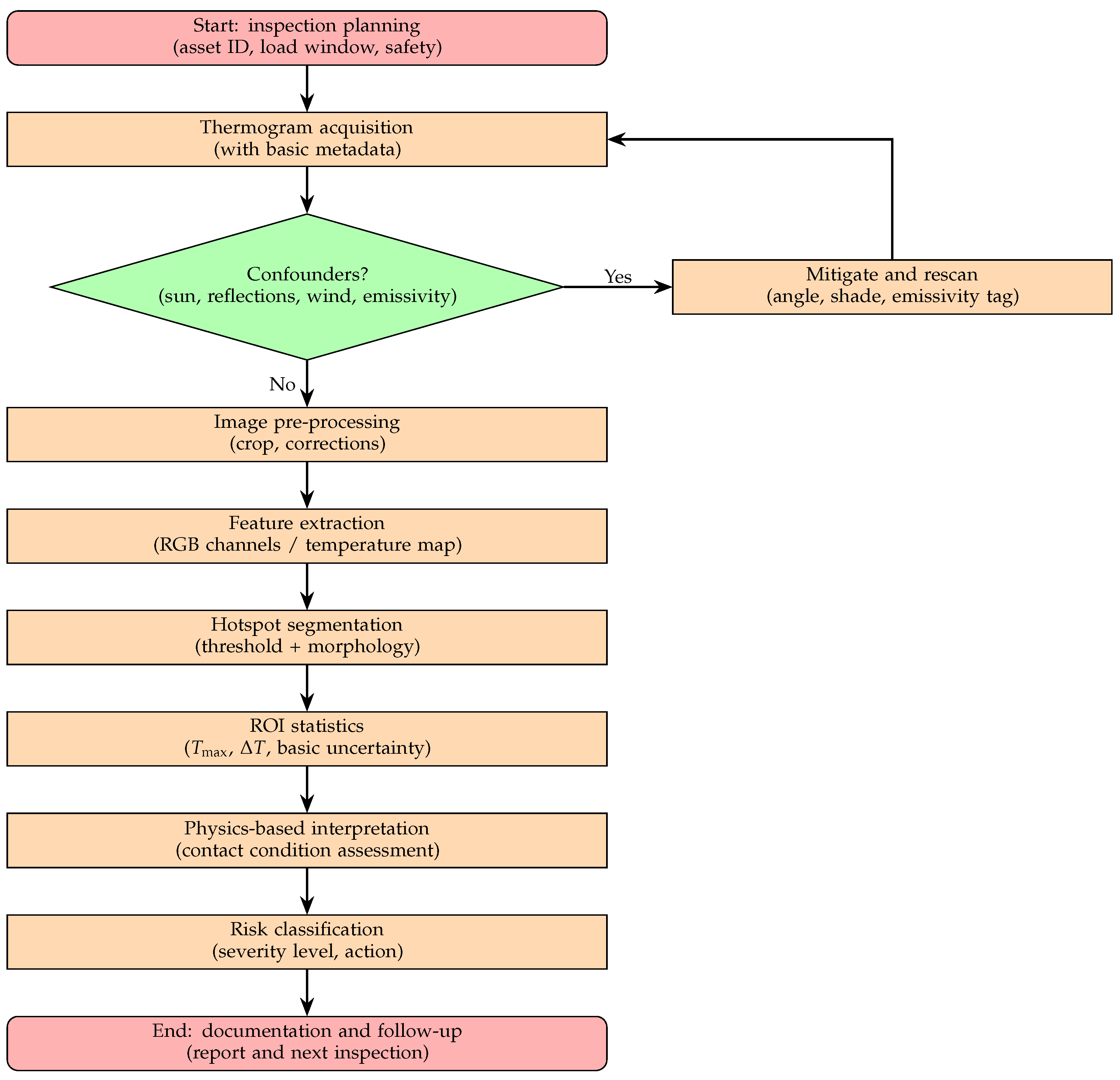
Figure 1 illustrates the high-level workflow adopted in this study, from inspection planning and thermogram acquisition to hotspot segmentation, ROI-based temperature statistics, physics-based interpretation, and final risk classification with recommended maintenance actions.
5. Results
For each case, this study computes (or plans to compute once inputs become available) the propagated temperature uncertainty and the derived uncertainties in and the Weibull parameter . The table below provides the reporting template; entries are marked “not computed” where the required covariances or are pending. In this field dataset, is derived from corrected surface temperatures (not pseudo-color), and larger at comparable load is interpreted as indicative of increased effective contact resistance ; a full quantitative estimate requires geometry/material/load data and is beyond the present scope.
To avoid overstatement, this study provides a statistical framing: for a binary detector tested on n cases with k detections, the point estimate is and a Wilson interval can be reported. For small n, a value of (i.e., ) admits a wide lower bound; e.g., with n moderate yields a substantial uncertainty. This study, therefore, moderates claims and reserves any fleet-level reliability statements for future work with labeled datasets and cross-validation. This study also outlines a power analysis to determine the n required to bound p within at confidence .
Table 4 summarizes, for each case, the propagated temperature uncertainty
, the resulting uncertainty in
, and the corresponding uncertainty in the Weibull characteristic life parameter
, together with the main assumptions for
and the dominant local sensitivity factors
.
This study explicitly states the time sampling schedule: current cases are single-visit inspections without longitudinal tracking. Consequently, the Weibull–Arrhenius prognosis remains a conceptual extension; prognostic claims based on a single snapshot are avoided. For assets under continuous monitoring, trend graphs of and over time will be reported in future work, in line with recent sensor/AI monitoring architectures that emphasize cadence and trend reliability.
Environmental Sensitivity and Confounding Factors
This study assesses how daytime solar heating, sky-reflected radiation, and emissivity variability can bias the temperature difference () and the inferred effective contact resistance (). The qualitative sensitivity matrix below guides risk reclassification when confounders are present.
Table 5 summarizes the qualitative effect of common environmental and radiometric confounders on the measured temperature
T (and therefore on
) and provides practical mitigation actions and rule-of-thumb reclassification guidance for field inspections.
The theoretical sections develop radiometry, contact resistance, electrochemical corrosion, and reliability (Weibull/Arrhenius). Here, this study makes the linkage explicit with one complete numerical example. Consider a hotspot reported at
°C with ambient
°C and emissivity set to
for oxidized metal. A simple emissivity correction (gray-body approximation) gives the true surface temperature in Kelvin as
with
K and
K, leading to
K (
°C). The corresponding
°C. While a full resistance estimate requires geometry and material data, qualitatively, a larger
at a similar load current indicates a higher effective contact resistance
. This study emphasizes that the full reliability parameters (e.g., Weibull shape
or Arrhenius activation energy
) are not fitted here; they are presented as a conceptual roadmap for future datasets with repeated observations and failure-time information.
Implemented in this dataset: radiometric correction, explicit ROI-based , and a thresholding–morphology pipeline yielding transparent hotspot masks. Presented as a roadmap: EIS-based resistance estimation, time-to-failure modeling, and fleet-level reliability scoring.
In the multi-site table below, the column labeled “Reliability” denotes the detection outcome for this illustrative sample. Because all listed cases were positively flagged by the study’s method, the observed detection proportion is ; to avoid a misleading “perfect” claim, this manuscript reports it with a Wilson 95% confidence interval (0.65–1.00). This does not represent asset reliability nor a generalizable performance metric; it only communicates that, within this small sample, the detection criterion was met.
It is also noted that extreme heating may arise from a short circuit or from a partial discharge with decreasing resistance, not only from a growing resistance. The results correspond to different thermographic images of transformer stations, in which the hotspot location is identified via image processing to determine whether it exceeds a suitable temperature threshold.
To eliminate subjective cut-offs, hotspot segmentation is specified as an adaptive procedure tied to this dataset. First, the per-image decision on the red channel uses Otsu’s threshold; when the histogram is low-contrast, a percentile fallback is applied (select pixels with ). Second, a chromatic guard suppresses warm backgrounds by enforcing and , with bounds anchored to the measured RGB samples: across 13 thermograms, clear hot regions exhibit and , whereas non-hot/warm backgrounds cluster around and ; thus, conservative dataset-based thresholds and are adopted. Connected components are filtered by a minimum-area prior estimated from the labeled subset, and each ROI reports max/mean and relative to a shaded reference patch. False-positive/false-negative rates (with precision, recall, F1, and IoU) are computed on the labeled frames, and a one-factor sweep perturbs the decision boundary by and gray levels around the Otsu split (and percentile points around ) to quantify sensitivity (IoU change, ROI centroid drift, and peak-temperature variation in °C). These dataset-anchored rules provide an objective statistical/algorithmic justification and reproducible settings under illumination variability.
Case 1: Substation A-04 Chimbacalle (Quito, Ecuador)
For this case, was not measured on-site. A follow-up will determine it using either step-current thermography or FEM with measured geometry, enabling a quantitative back-out of with uncertainty bounds.
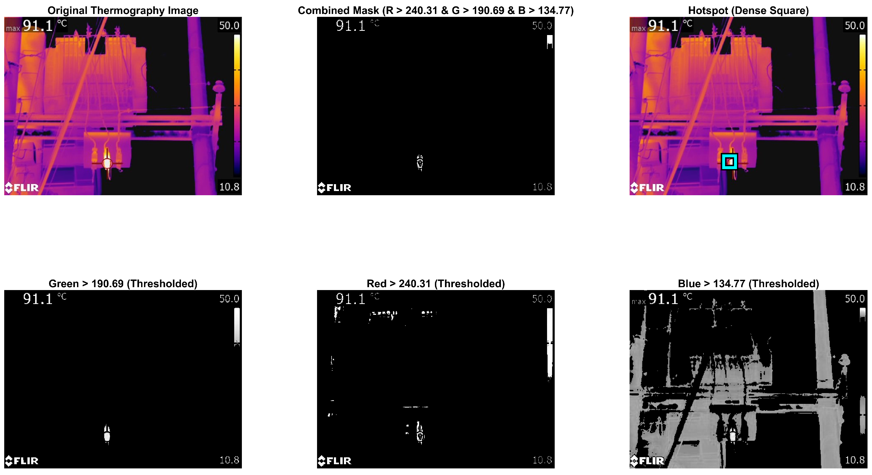
The thermographic image shows the hot spot where the following coordinates are obtained: [X,Y] [90 60] and also the coordinates in [R, G, B] [254 230 204], thus locating the potential failure in the transformer and the affected element, such as the NH fuse; this will favor the maintenance of the equipment, hence ensuring its efficiency and reliability to prevent future damage or power outages.
Processing summary (Case 1). For the radiometric JPEG, the algorithm splits the image into RGB channels and applies fixed, per-channel thresholds in uint8 space: , , . Pixels satisfying all three conditions form the combined mask. To avoid overlay artifacts, non-informative borders are excluded (top/bottom captions, the left logo, and the right color bar), and a 3 × 3 neighbor filter (requires ≥4 neighbors) removes isolated pixels. A sliding square window (∼5% of the larger image side) builds a density map over the cleaned mask; the window centered at the maximum density defines the hotspot region. The first row of thermography_1.png displays, in order, the original frame, the combined mask, and the original with a high-contrast bounding square (black outline with cyan inner stroke) centered on the densest hotspot. The second row shows the thresholded Green, Red, and Blue channels, respectively. All panels are exported at 600 dpi.
Figure 2 shows, in the upper row, the original thermographic image, the combined mask obtained after thresholding, and the hotspot identification overlaid on the original image. In the lower row, the figure presents the decomposed color-channel images (Green, Red, and Blue), after applying the corresponding thresholding step.
Table 6 reports the matrix-structure parameters of the thermographic image used in Case 1 and its derived arrays. These parameters document the data structure of the processed image and support reproducibility of the pipeline.
As a result of the thermographic image through image processing, the following coordinates were obtained in [X Y] [49–60 : 85–90], which will allow finding the hot spot, obtaining precise data, and the exact location of the transformer fault, as shown in
Table 7.
Case 2: Abel Meléndez and Napo Street (Quito, Ecuador)
For this case, was not measured on-site. A follow-up will determine it step-by-step with current thermography or FEM with measured geometry, enabling quantitative back-out of with uncertainty bounds.
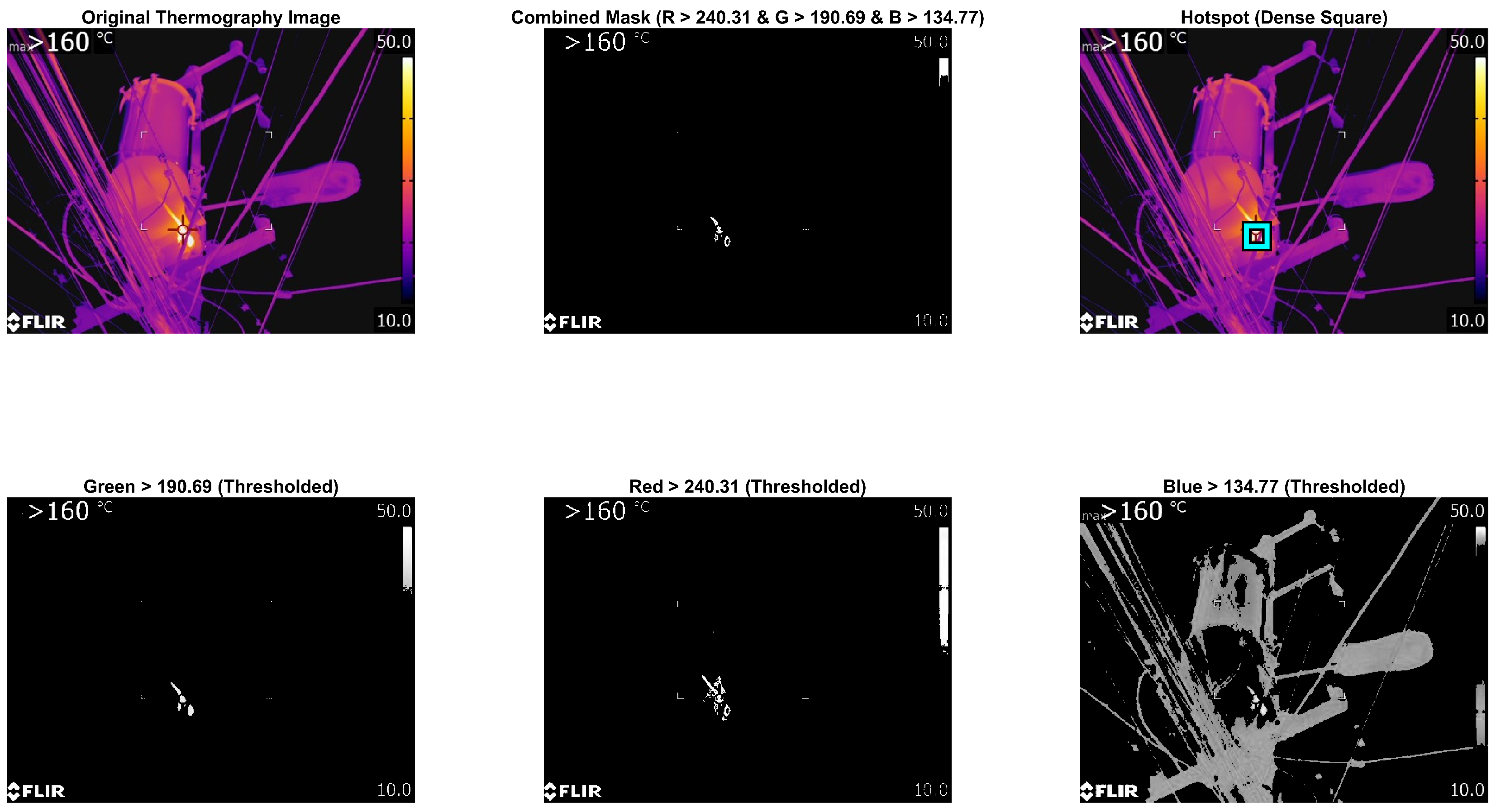
The thermographic camera results show an abnormal temperature of 91.1 degrees Celsius, exceeding the minimum and safety limits and falling outside acceptable operating conditions. By means of the image processing technique, it is possible to appreciate the fault quickly and avoid overloads and potential fires in the transformer; that is why RGB images are obtained to appreciate the fault, and also the following coordinates will be obtained: [X,Y] [244 334] and, in the same way, the coordinates in [R, G, B] [111 22 16]. The matrix mentioned above was generated by the program; therefore, the thermographic image was dimensioned as shown in
Table 3.
Consequently, from the precise data obtained and the coordinates in [X,Y] [244 334] the exact location of the transformer fault will be obtained; therefore, it will allow finding the hot spot, and it will be observed in
Table 4.
Processing summary (Case 2). The same pipeline is applied: RGB channel split; hard thresholds , , ; logical AND to form the combined mask; border exclusion (top/bottom text, left logo, right color bar); 3×3 neighbor cleanup (≥4 neighbors). A sliding square window (∼5% of the larger side, clamped for scale) produces a density map; the peak locates the most concentrated set of 1s in the mask. The first row of thermography_2.png presents the original image, the combined mask, and the hotspot visualization with the high-contrast square. The second row presents the thresholded Green, Red, and Blue channels. All images are rendered at high resolution (600 dpi) to preserve measurement detail.
Figure 3 shows, in the upper row, the original thermographic image, the combined mask obtained after thresholding, and the hotspot identification overlaid on the original image. In the lower row, the figure presents the decomposed color-channel images (Green, Red, and Blue), after applying the corresponding thresholding step.
Table 8 reports the matrix-structure parameters of the thermographic image used in Case 2 and its derived arrays. These parameters document the data structure of the processed image and support reproducibility of the pipeline.
As a result of the thermographic image through image processing, the following coordinates were obtained in [X Y] [329–334 : 238–242], which will allow finding the hot spot, obtaining precise data, and the exact location of the transformer fault, as shown in
Table 9.
Finally,
Table 10 and
Table 11 presents the results obtained using the image-processing technique. Finally, it presents evidence from the study, analyzing faults in the transformers at the primary A-04 Chimbacalle substation.
Overview. The results draw from a field dataset of over 500 thermograms acquired on distribution assets and reported with full radiometric context (camera settings, emissivity, distance, shaded ). Apparent readings are converted to surface temperature, and is computed against a shaded reference ROI. Hotspot masks are obtained with an adaptive pipeline (per-image Otsu threshold with a percentile fallback and chromatic guards), yielding consistent ROIs and statistics (max/mean). To make performance transparent, the section juxtaposes fault-positive cases—where elevated and contact locations indicate degradation—with fault-negative cases under comparable ambient/load conditions where the method rightly refrains from flagging faults.
6. Discussion: Model-Based Interpretation and Implications for Corrosion and Materials Degradation
Relationships based on mixed potential, Stern–Geary, and Randles circuits assume specific interface behaviors. This study operates within ranges where linearizations are valid: moderate overpotentials, currents within the linear EIS regime, and temperatures close to those for which parameterizations were obtained. Deviations (e.g., severe polarization, surface films, or pollutant loads outside calibration) can bias estimates of and ; when such conditions are suspected, the analysis refrains from numerical inference and recommends direct electrochemical characterization.
This study hypothesizes (and prior literature suggests) that tightening under mechanical degradation reduces . To validate this, this study defines an experimental sequence: (i) baseline thermogram and DC resistance/EIS; (ii) torque procedure with calibrated wrench and tolerance logging; (iii) immediate post-torque DC/EIS; (iv) 24–72 h follow-up. The evolution of and across these steps will be reported with measurement tolerances. This was not executed in the current dataset and is listed as a limitation.
The concentrated model of Equation (
10) applies to connectors in which heat generation is dominated by localized contact resistance and the accessible surfaces are radiometrically observable: bolted/clamped lugs, compression terminals, bus joints, and bushing terminals with minimal shrouding. Extension to geometries with distributed heating (e.g., long cable runs, encapsulated joints) or strong internal convection requires either a refined thermal network or FEM calibration.
Generalizability to Different Environments and Equipment Types
The method is designed to be transferable, but its decision quality depends on acquisition conditions and the infrared camera’s temperature rendering. First, different climates (humidity, pollution, salt deposition, and diurnal temperature swings) modify both corrosion kinetics and thermographic confounders (time of wetness, solar loading, and wind cooling). Consequently, the same
threshold can correspond to different degradation stages unless emissivity, reflected temperature, and operating current are controlled or uncertainty-bounded (Equations (
13) and (
16)). Second, different equipment types (transformer bushings, bolted bus joints, compression lugs, clamps, and switchgear contacts) present different heat-sink paths and therefore different
; a calibration (step-current thermography or FEM) is required before comparing
across geometries. Third, the RGB decomposition step is camera- and palette-dependent: pseudo-color exporters may map temperature to RGB using different colormaps, making fixed RGB thresholds non-universal. For this reason, the manuscript treats RGB-channel thresholding as a surrogate to be used only when radiometric temperature fields are unavailable, and it recommends validating the thresholds per camera/export mode using the performance metrics in
Section 4.
To strengthen sensitivity reporting beyond ideal emissivity and capture-distance conditions, the workflow includes (i) repeated captures at two distances within the safe operating window, (ii) a bracket on emissivity (e.g.,
for oxidized metal) to bound temperature bias, and (iii) a “confounder-present” rule that triggers rescan or conservative reclassification (
Table 5). These steps explicitly target generalization across typical field variability.
This study’s approach complements recent hybrid FEM–AI and sensor–AI monitoring work by explicitly exposing the physics-to-image pathway and the measurement assumptions. This study differs in (i) focusing on radiometric transparency (documented camera settings, emissivity, and corrections), and (ii) prioritizing uncertainty and sensitivity reporting before model scoring. This positioning helps bridge thermographic diagnostics with reproducible, bias-aware hybrid models.
This study revisits Holm’s contact theory, corrosion kinetics, and reliability models to interpret observed hotspots. Where concrete data exist (single-visit thermograms and ROI statistics), this study anchors the discussion to the reported and corrected temperatures. Elements that require repeated measurements or dedicated instrumentation (e.g., EIS for , retorquing-and-reinspection studies, or Weibull fits across a fleet) are explicitly framed as future work, not as validated components of the present dataset.
The mathematical framework in
Section 2 explains the empirical thermograms by explicitly linking contact degradation and corrosion kinetics to temperature rise. First, Equations (
8)–(
10) indicate that small increases in
(due to oxide films or loss of clamping force) produce quadratic increases in dissipated power with the operating current. Second, EIS-derived
values feed Equation (
2) to estimate
, which in turn allows computing thickness-loss rates via Equation (
4). Third, the Arrhenius form (
5) rationalizes the observation that assets in warmer microclimates or subject to solar loading deteriorate faster. Finally, uncertainty budget Equations (
13)–(
17) identify the parameters that must be controlled in field surveys (e.g., emissivity and reflected temperature) to maintain decision-grade accuracy.
Case Interpretation: For the reported case studies (Sections on Substation A-04 Chimbacalle and Abel Meléndez), the measured hot spots can be translated into estimates of
using Equation (
10) once
is characterized (by simple step-current tests or finite-volume thermal models). Combining
trends with periodic EIS or DC resistance measurements allows separation of purely mechanical looseness from chemically driven film growth. If
decreases after retorquing, mechanical causes dominate; if not, corrosion/contamination is likely predominant, and cleaning and surface protection are warranted.
Risk and Maintenance Prioritization: The Weibull–Arrhenius model (Equation (
18)) produces a probability-of-failure forecast conditioned on the observed
. Assets with high
(hence low
) should be scheduled for immediate maintenance; those with moderate
qualify for closer monitoring and cleaning; assets with low
can remain on routine inspection cycles. This quantitative triage exceeds qualitative color-thresholding alone and is aligned with reliability-centered maintenance practices [
18].
This study hypothesizes—consistent with prior reports—that re-torquing mechanically degraded connectors reduces , but matched before- and after-electrical data are not available in the present field set. To validate this prospectively (without altering the journal template), the discussion frames a future protocol: (i) acquire a baseline thermogram with shaded , fixed emissivity and distance, and logged load I; (ii) measure four-wire DC resistance (resolution ≤1 m) and, where clearance and safety permit, a short EIS sweep (e.g., 10 kHz–0.5 Hz) to estimate ; (iii) apply re-torque using a calibrated wrench at the manufacturer’s nominal value (tolerance ±4% full-scale), either in a single step or in 10% increments; (iv) allow 5–10 min thermal stabilization at comparable load/ambient; and (v) repeat DC/EIS and thermography under the same settings and again at 24–72 h. The evolution of , four-wire , and (when available) EIS-derived will be reported with instrument tolerances and propagated uncertainty, providing a defensible before/after assessment of tightening effects; until then, this mechanism is treated as a limitation and a target for future validation.