A Hybrid Variational Mode Decomposition, Transformer-For Time Series, and Long Short-Term Memory Framework for Long-Term Battery Capacity Degradation Prediction of Electric Vehicles Using Real-World Charging Data

Abstract

Considering the nonlinear trends, multi-scale variations, and capacity regeneration phenomena exhibited by battery capacity degradation under real-world conditions, accurately predicting its trajectory remains a critical challenge for ensuring the reliability and safety of electric vehicles. To address this, this study proposes a hybrid prediction framework based on Variational Mode Decomposition and a Transformer–Long Short-Term Memory architecture. Specifically, the proposed Variational Mode Decomposition–Transformer for Time Series–Long Short-Term Memory (VMD–TTS–LSTM) framework first decomposes the capacity sequence using Variational Mode Decomposition. The resulting modal components are then aggregated into high-frequency and low-frequency parts based on their frequency centroids, followed by targeted feature analysis for each part. Subsequently, a simplified Transformer encoder (Transformer for Time Series, TTS) is employed to model high-frequency fluctuations, while a Long Short-Term Memory (LSTM) network captures the long-term degradation trends. Evaluated on charging data from 20 commercial electric vehicles under a long-horizon setting of 20 input steps predicting 100 steps ahead, the proposed method achieves a mean absolute error of 0.9247 and a root mean square error of 1.0151, demonstrating improved accuracy and robustness. The results confirm that the proposed frequency-partitioned, heterogeneous modeling strategy provides a practical and effective solution for battery health prediction and energy management in real-world electric vehicle operation.

1. Introduction

With the increasingly severe environmental pollution and energy shortages caused by extensive consumption of fossil fuels, the global energy system is accelerating its transition toward green and low-carbon development [1]. In this context, electric vehicles (EVs) have become an important development direction for road transportation. As the core energy storage component of EVs, lithium-ion batteries directly determine vehicle performance, safety, and service life [2]. However, battery capacity degradation during long-term operation is inevitable and poses critical challenges to EV reliability and lifetime. Therefore, establishing accurate and reliable prediction models for battery pack capacity degradation is of great significance for practical EV applications and sustainable industrial development. Compared with individual cells, battery pack degradation is considerably more complex. This complexity arises from cell-to-cell inconsistencies, different aging rates, and interactions among cells during operation [3]. In addition, battery packs operate under diverse usage patterns, environmental conditions, and charging–discharging behaviors in real-world scenarios [4]. The coupling of these intrinsic and extrinsic factors makes accurate prediction of battery pack capacity degradation particularly challenging. Existing studies on battery capacity degradation prediction can generally be divided into two categories: electrochemical mechanism-based modeling methods and data-driven approaches [5]. Electrochemical models focus on describing internal physicochemical processes and offer strong interpretability, whereas data-driven methods rely on historical operational data and are more suitable for complex real-world battery pack conditions.

Electrochemical mechanism-based modeling constructs mathematical representations of battery aging by linking measurable external signals with internal physicochemical processes. Equivalent Circuit Models (ECMs) are widely used for State-of-Health (SOH) estimation by tracking parameter evolution during aging, due to their simple structure and low computational cost [6,7,8]. However, ECMs show limited accuracy in representing complex degradation behaviors and are sensitive to parameter initialization. To improve estimation performance under dynamic conditions, ECMs are often combined with state estimators such as Extended Kalman Filters (EKFs). Representative studies include coupled electro-thermal aging models [9], multi-scale EKF-based SOC and capacity tracking [10], and dual Kalman filter frameworks for multi-state monitoring [11]. While these methods balance robustness and real-time capability, they require careful model design and parameter tuning. Beyond equivalent circuits, electrochemical models establish relationships between SOH and internal states through charge transfer and reaction kinetics. Existing studies have explored hybrid physical–ECM frameworks [12], parameter optimization of pseudo-two-dimensional (P2D) models [13], and iterative observer-based estimation schemes [14]. Despite their strong interpretability, the complexity of parameter identification and high computational burden limit their applicability in large-scale or real-time scenarios.With advances in data acquisition and computing power, data-driven approaches have gained increasing attention. These methods directly extract degradation patterns from operational data such as voltage, current, temperature, and capacity. Feature extraction strategies include Incremental Capacity Analysis (ICA) under different charging conditions [15,16], differential voltage analysis during charging [17,18], and multidimensional feature construction across multiple operating stages [19], highlighting the application-dependent nature of feature engineering.Regarding modeling techniques, traditional machine learning methods are commonly adopted due to their ease of implementation. Random forest regression [20], support vector regression with feature processing [21,22,23,24], XGBoost [25], and Gaussian process regression for partial charging data [26,27] have all been applied to SOH estimation tasks. More recently, deep learning models have been widely explored for complex time-series modeling. LSTM [28] and GRU [29] architectures are commonly used for capacity prediction, often combined with evolutionary optimization algorithms [30,31] or integrated network designs [32,33]. For higher-dimensional inputs, CNN–LSTM hybrid models have been proposed to jointly capture spatial and temporal characteristics [34], with further hyperparameter optimization using metaheuristic algorithms [35]. To overcome limitations in local feature extraction and feature anisotropy, Transformer-based architectures have also been introduced for multi-step battery capacity prediction, including models with enhanced convolutional structures [36], sparse self-attention and multi-scale feature fusion for long-term SOH forecasting [37], as well as Transformer-based frameworks targeting real-time SOH estimation in battery management systems [38].

Despite these advances, model performance remains highly dependent on feature quality and data availability. The coexistence of regeneration effects, gradual degradation, and measurement noise further challenges conventional recurrent and convolution-based models in capturing long-term degradation trends under non-stationary conditions. To address the highly nonlinear nature of raw capacity data and capacity regeneration phenomena, researchers have introduced modal decomposition techniques to extract representative intrinsic mode functions (IMFs) and residuals from original capacity signals [39]. For instance, Huang et al. [40] incorporated Complete Ensemble Empirical Mode Decomposition with Adaptive Noise (CEEMDAN)-decomposed capacity modes into a feature fusion framework, designing a multi-module integrated bidirectional feedback spatiotemporal attention neural network for multi-step SOH prediction. This approach enhanced time–frequency resolution to some extent and demonstrated spatiotemporal modeling capabilities. However, each prediction requires CEEMDAN decomposition of historical SOH data in practical applications, and the inherent uncertainty of decomposition compromises model stability and timeliness. Liu et al. [41] employed Empirical Mode Decomposition (EMD) to decompose raw data into multiple IMFs and residuals, using LSTM for residual estimation and Gaussian Process Regression (GPR) to fit other IMFs. Aging tests across diverse batteries confirmed reliable results even during early degradation stages. To prevent information leakage during decomposition, Li et al. [42] proposed a similarity-day-extended EMD method. While EMD serves as an effective nonlinear signal processing tool, it suffers from mode mixing when analyzing complex battery degradation patterns. VMD overcomes these limitations by effectively separating distinct IMFs from nonlinear signals [43]. Chen et al. [44] optimized VMD parameters via Particle Swarm Optimization (PSO) for capacity decomposition, eliminating residuals while maximally preserving sequence information, followed by convolutional networks for denoised capacity degradation prediction. Other studies utilize decomposed components as multi-channel inputs for deep models: Chen et al. [45] combined multi-population evolutionary whale-optimized VMD with Transformer architecture, feeding all IMFs into the network. Similarly, Wang et al. [46] input VMD-derived IMFs into attention-enhanced Temporal Convolutional Networks (TCNs). These methods, however, face significantly increasing model complexity with growing IMF quantities.To mitigate this issue, Fu et al. [47] introduced permutation entropy (PE) to quantify the complexity of each IMF, combining those with similar complexity levels to reduce model input dimensionality, then separately modeling and predicting the aggregated components. Similarly, Li et al. [48] categorized IMFs into high-frequency and low-frequency groups based on zero-crossing rates, constructing distinct neural networks for each category to further compress model scale. It should be noted that while zero-crossing rate-based partitioning effectively separates short-term fluctuations from long-term trends in capacity sequences, these rapid fluctuation components typically exhibit poor regularity and present substantial modeling challenges. Although these methods demonstrate strong predictive performance across multiple public datasets, critical considerations remain. Battery pack capacity degradation manifests as a long-term, gradual process where short-term changes are often insufficiently pronounced, necessitating further investigation into optimal prediction horizon selection. Additionally, the physical mechanisms and behavioral significance underlying high-frequency and low-frequency components in capacity sequences remain inadequately understood, constraining improvements in model interpretability. Most importantly, research on battery pack degradation patterns under real-world electric vehicle operating conditions remains underdeveloped, being currently unable to satisfy the dual requirements of accuracy and reliability for practical deployment.

To address the above challenges, this paper proposes a VMD–TTS–LSTM framework for long-horizon capacity degradation prediction of in-service EV battery packs. Unlike existing VMD-based methods that either model all decomposed IMFs or aggregate them using empirical complexity measures, this study introduces a frequency-domain partitioning strategy that separates short-term disturbances from long-term degradation behaviors to support heterogeneous modeling. The proposed framework integrates frequency-domain decomposition with heterogeneous time-series modeling, aiming to improve prediction accuracy and interpretability under real-world operating conditions. The main contributions of this work are summarized as follows:

• A frequency-domain-based partitioning strategy is proposed to decompose nonlinear battery capacity degradation sequences. By applying VMD and aggregating the decomposed modes into high- and low-frequency components, the proposed strategy facilitates more effective feature representation of short-term fluctuations and long-term degradation trends.
• A simplified Transformer-based encoder architecture for time-series prediction, termed Transformer for Time Series (TTS), is introduced. By retaining only the encoder and removing the decoder and autoregressive mechanism, a non-autoregressive multi-step prediction scheme is established, which reduces model complexity and mitigates error accumulation while preserving global temporal modeling capability.
• A frequency-partitioned feature analysis and heterogeneous modeling framework is developed. Different feature correlation screening and modeling strategies are designed for the high- and low-frequency components, and their predictions are jointly integrated to achieve accurate long-horizon capacity forecasting.

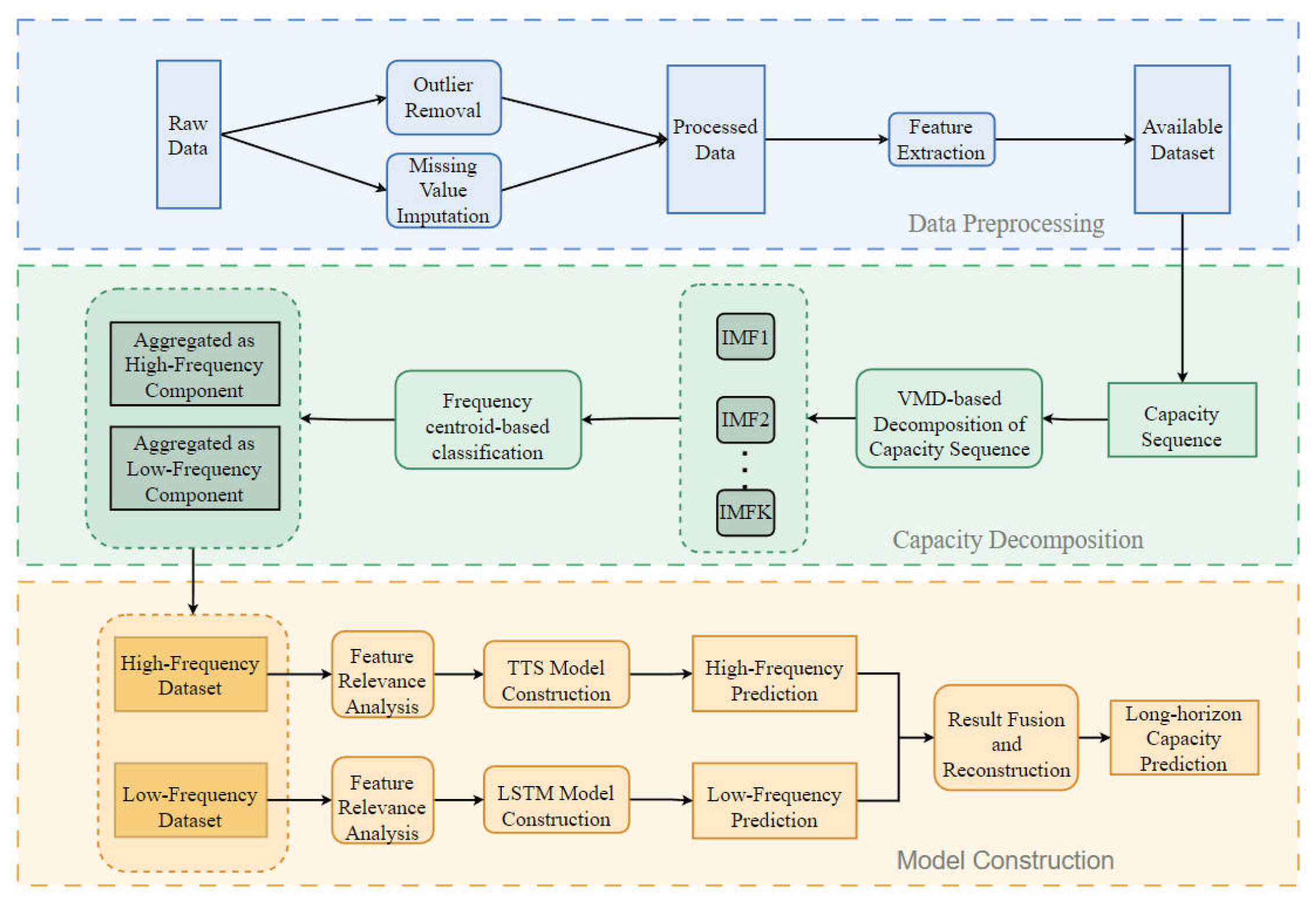
Figure 1 presents an overview of the proposed framework, including data preprocessing, capacity decomposition, feature analysis, and model construction.

The remainder of this paper is organized as follows. Section 2 introduces the commercial EV dataset and the capacity extraction procedure. Section 3 describes feature extraction and component-specific feature analysis. Section 4 presents the proposed models and training strategy. Section 5 reports the experimental setup and comparative results. Section 6 concludes the paper.

2. Data Analysis

2.1. Data Introduction

This study analyzes a power battery charging dataset from 20 commercial electric vehicles (designated #1–#20) provided by Deng et al. [49]. All vehicles are equipped with lithium-ion battery modules rated at 145 Ah. The data acquisition system collects real-time charging parameters through battery management systems (BMS), with transmission handled via Controller Area Network (CAN) buses. Experimental data spans 29 months and includes battery pack voltage, charge/discharge currents, maximum/minimum cell voltages, maximum/minimum cell temperatures, and available energy.

Table 1. Dataset overview of the 20 commercial electric vehicles.

ID	Start	End	Data (k)	Cycles	ID	Start	End	Data (k)	Cycles
1	26 July 2019	15 November 2021	854.6	1542	2	25 July 2019	15 November 2021	841.8	1520
3	26 July 2019	15 November 2021	802.9	1546	4	25 July 2019	15 November 2021	844.5	1463
5	26 July 2019	15 November 2021	832.2	1503	6	25 July 2019	15 November 2021	815.2	1463
7	26 July 2019	15 November 2021	808.8	1481	8	26 July 2019	15 November 2021	798.5	1466
9	23 July 2019	15 November 2021	792.1	1431	10	24 July 2019	15 November 2021	728.9	1309
11	26 July 2019	15 November 2021	809.5	1456	12	22 July 2019	16 November 2021	825.5	1483
13	26 July 2019	15 November 2021	818.4	1425	14	26 July 2019	15 November 2021	793.1	1441
15	25 July 2019	15 November 2021	705.0	1253	16	23 July 2019	15 November 2021	819.6	1534
17	25 July 2019	15 November 2021	767.9	1389	18	26 July 2019	15 November 2021	856.2	1524
19	24 July 2019	15 November 2021	778.7	1424	20	26 July 2019	15 November 2021	807.5	1470

provides the detailed information for each vehicle. The table includes four key columns for each vehicle. The Start and End columns show the data collection period. The Data (k) column represents the number of data points in thousands. The Cycles column indicates the total charging cycles recorded. The specific method for identifying and segmenting individual charging cycles is detailed in Section 2.2.

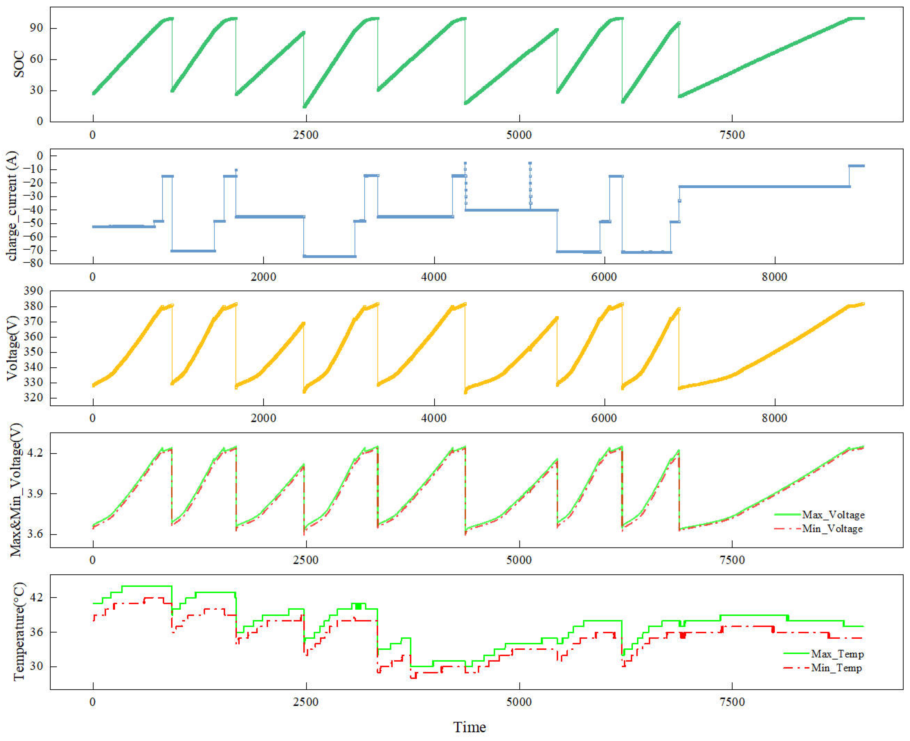
As shown in Figure 2, the first nine extended charging cycles of Battery Pack #1 exhibit characteristic multi-stage constant-current charging behavior. All vehicles in the dataset are commercial electric taxis operating within the same city. This ensures comparable macro-level operating conditions such as climate and charging infrastructure. Nevertheless, clear differences exist among individual vehicles in terms of usage intensity, charging frequency, and operational schedules. These differences lead to heterogeneous capacity degradation behaviors across vehicles. These behaviors cannot be explicitly categorized using predefined labels. The coexistence of similar operating environments and diverse usage patterns provides a suitable testbed. This testbed evaluates the robustness of the proposed model under realistic inter-vehicle variability.

2.2. Labeled Capacity Estimation

Precise extraction of labeled capacity values from raw charging data is essential for establishing an accurate battery capacity degradation prediction model. The labeled capacity of a battery is typically defined as the total charge released from a fully charged state to the cutoff voltage under specified standard test conditions (including discharge rate, ambient temperature, cutoff voltage, etc.). Since battery packs usually exhibit high Coulombic efficiency during operation, the charging capacity during the charging process can also be used as an approximate indicator of the battery pack’s true capacity. As the number of cycles increases, the labeled capacity of the battery pack gradually degrades. When the capacity drops below 80% of the initial rated capacity, it is generally considered to have reached the end-of-life criterion. Therefore, accurately obtaining the labeled capacity of a battery pack is of great significance for lifespan evaluation and degradation modeling. In practical research, many scholars use the Ampere-hour integration method to calculate battery capacity by integrating the current over time during the charging process. However, this method requires high-precision current sampling and a relatively complete charging segment. In real-world applications such as electric vehicles, due to the randomness and uncertainty of charging behavior, battery packs often cannot guarantee each charge as a complete “full charge–discharge” cycle, making it difficult to directly apply traditional methods. To address this issue, this paper adopts the Ampere-hour integration-based capacity estimation formulation proposed in [50], which estimates the effective capacity after each charge under non-standard charging conditions. This method does not require a complete charging process to achieve an approximate estimation of capacity, offering strong practicality and robustness, as defined in Equation (1):

$$C={\displaystyle \frac{-{\int }_{t_1}^{t_2}I\left(t\right)dt}{SO{C}_{t_2}-SO{C}_{t_1}}}$$

(1)

where $t_1$ denotes the charging start time, $t_2$ denotes the charging end time, $I\left(t\right)$ represents the current as a function of time, and $SOC$ is the state of charge of the battery.

In the above formula, the battery capacity is defined as the ratio between the integrated charging current and the corresponding variation in state of charge (SOC). The accuracy of the estimated capacity is therefore highly dependent on the reliability of SOC measurements, and larger SOC intervals during a charging process generally lead to more accurate capacity estimation. In this study, SOC is treated as an auxiliary state variable observed during the charging process and is not used as an independent modeling or prediction target. Instead, SOC information supports capacity estimation by providing a normalized charge progression reference. Considering the non-ideal and irregular nature of real-world electric vehicle charging data, to ensure the reliability of the capacity labels derived from real-world charging data, we implement several data filtering and smoothing steps during the label construction process. First, when the time interval between two consecutive recorded data points exceeds 30 s, the corresponding charging record is regarded as discontinuous and is divided into separate charging processes to avoid integration errors. Second, charging events with an SOC variation smaller than 30 are excluded, as small SOC intervals tend to amplify estimation uncertainty and noise. Even after these filtering steps, the capacity estimated from a single charging event may still exhibit noticeable fluctuations due to charging current variability, operational disturbances, and measurement uncertainty. To further enhance the robustness of the capacity labels, the estimated capacities are averaged over every ten consecutive charging cycles to construct nodal capacity values. This ten-cycle averaging serves as a temporal smoothing strategy at the label construction stage. It suppresses short-term stochastic variations while preserving the underlying long-term degradation trend of the battery pack. The ten-cycle window length is empirically selected as an engineering trade-off between temporal resolution and label stability, reflecting typical real-world EV charging frequency. This averaging preserves the broader degradation trend.

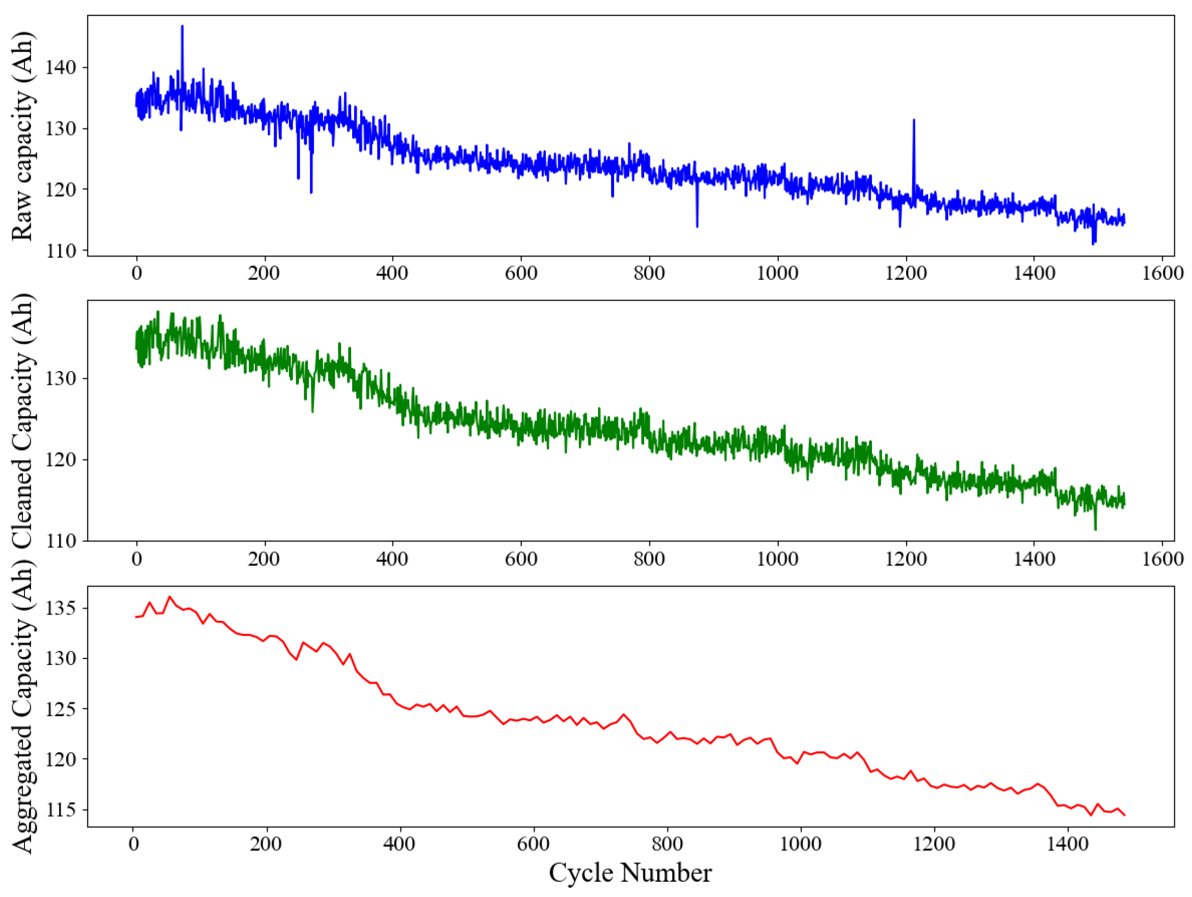
Figure 3 presents the original labeled capacity data of Vehicle #2 calculated using Equation (1). As observed, the sequence exhibits numerous outliers and pronounced fluctuations, indicating the presence of estimation noise and computational errors. To eliminate such disturbances, a $3\sigma$-based outlier detection method under a sliding window was applied, removing anomalous values outside the acceptable range. The middle portion of Figure 3 illustrates the denoised capacity data, which shows significantly reduced fluctuation and improved smoothness. Furthermore, to better characterize the underlying degradation trend, a sliding window averaging was conducted on the cleaned data. The bottom section of Figure 3 displays the resulting smoothed capacity degradation curve, which clearly reveals a long-term downward trend as the number of charging cycles increases.

2.3. Frequency-Based Capacity Decoupling

In commercial electric vehicle battery packs, capacity degradation is not only influenced by the inherent chemical properties of the battery cells but is also closely related to external factors such as operating conditions and usage patterns. To thoroughly investigate the degradation characteristics of the capacity sequence across different frequency components and their potential influencing factors, this study introduces VMD to decouple the capacity sequence in the frequency domain.

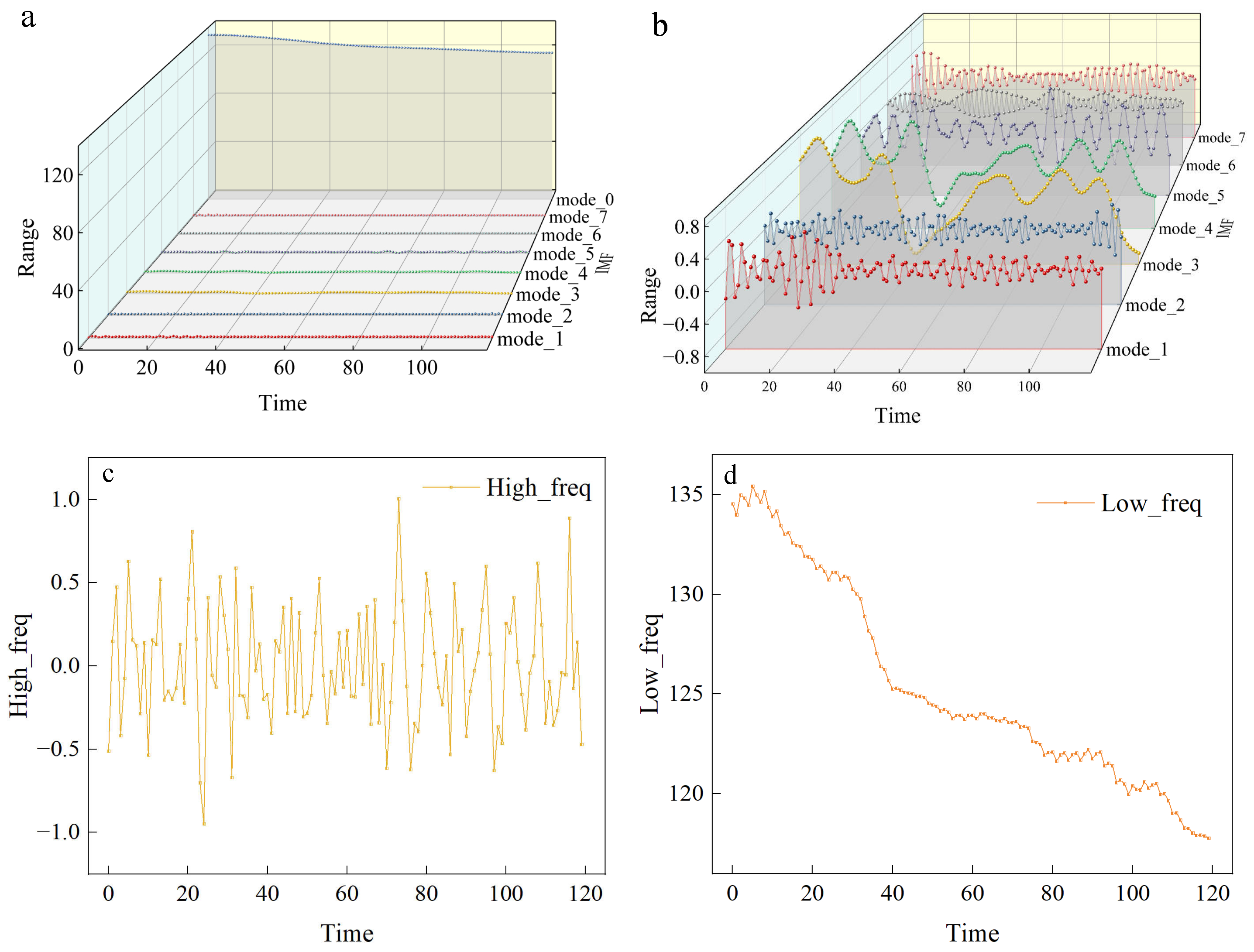
In this study, for the capacity sequence of each electric vehicle, a joint optimization of the number of modes (K) and the penalty factor ($\alpha$) was performed using grid search within the ranges of $K\in [2,8]$ and $\alpha \in [100,2000]$. The optimal parameter combination was determined by minimizing the reconstruction error between the sum of the decomposed IMFs and the original capacity sequence. The IMFs obtained from the decomposition of Vehicle #1 are shown in Figure 4a, where a dominant trend component and multiple fluctuation components of varying degrees can be observed. The trend component, which accounts for the majority of the sequence’s energy, reflects the long-term degradation trend of the battery pack’s capacity. Meanwhile, certain fluctuation components, such as IMF3 and IMF4, exhibit relatively smoother and more regular variation patterns, as shown in Figure 4b. To categorize these components into high- and low-frequency groups, this study calculates the frequency centroid [51] of each IMF. Based on a predefined threshold, the trend component and some mid-to-low-frequency fluctuation components with lower frequency centroids are classified as low-frequency components, while the remaining modes are categorized as high-frequency components. Ultimately, the high-frequency and low-frequency capacity sequences are constructed, as depicted in Figure 4c,d.

3. Feature Engineering

3.1. Feature Extraction

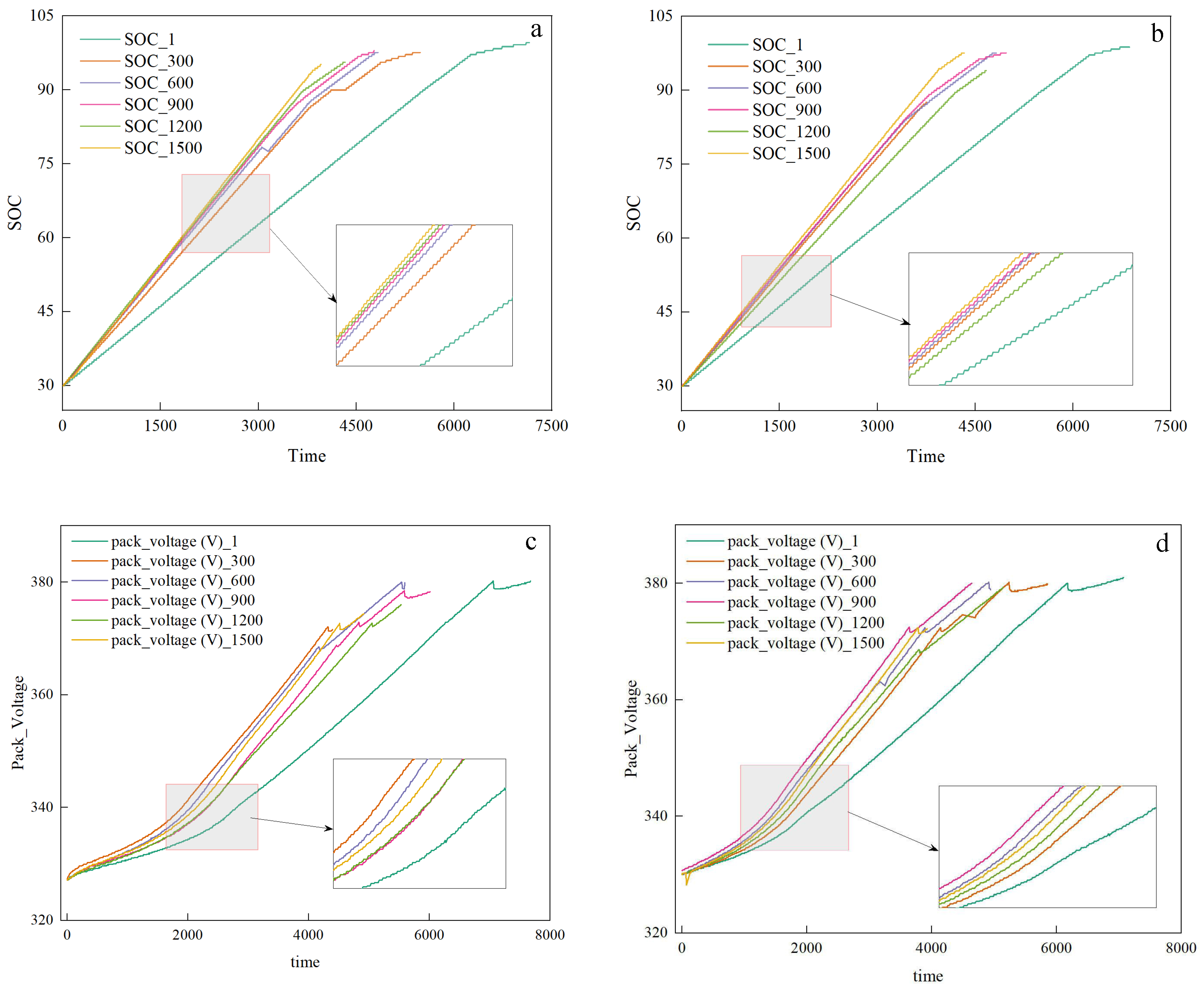
To more accurately characterize the capacity degradation process of battery packs, this study conducts detailed feature extraction for each charging cycle based on collected key operational parameters. Specifically, the extracted features include the maximum, minimum, mean, and standard deviation of each parameter during the charging process, as well as the duration of each charge, charging capacity, and the initial SOC, final SOC, and SOC difference. However, relying solely on these static statistical features may still be insufficient to fully capture the dynamic evolution of battery capacity. As shown in Figure 5, even when the initial SOC remains consistent, the SOC curve exhibits an overall leftward shift with increasing charge cycles, while the voltage curve, after shifting left to a certain extent, begins to fluctuate in the middle range. This indicates nonlinear changes in charging behavior and internal reactions during battery degradation.

To address this, in addition to basic statistical features, this study further introduces dynamic features such as the SOC change rate, voltage change rate, maximum cell voltage change rate, and minimum cell voltage change rate during each charging process to characterize finer dynamic variations. On the other hand, since the capacity label in this study is derived from the average of multiple adjacent charging cycles to reduce noise from capacity fluctuations, the feature construction must align with this approach. Simply averaging features across charging cycles may obscure behavioral differences and fail to fully reflect the impact of charging patterns on capacity degradation. Therefore, this study treats the multiple charging cycles used to construct the capacity label as a single data point and extracts five key features—charging duration, charging capacity, initial SOC, final SOC, and SOC difference—calculating their maximum, minimum, mean, and standard deviation to comprehensively reflect the upper and lower bounds of charging behavior. For other features, the mean values are taken. Ultimately, this study constructs a total of 59 feature variables to serve as potential inputs for the model.

3.2. Correlation Analysis

This study utilizes the Spearman’s rank correlation coefficient to analyze the correlation between extracted features and the high/low frequency components of the capacity sequence. This method operates on sample ranks rather than raw values, effectively mitigating the influence of outliers while demonstrating strong adaptability to nonlinear relationships—making it particularly suitable for real-world data scenarios with noise interference. Compared to Pearson correlation and similar methods, Spearman correlation does not require linear relationships between variables, as it can detect correlations as long as a monotonic trend exists. This characteristic renders it more appropriate for complex, nonlinear battery capacity degradation feature selection tasks [52]. The calculation formula is presented in Equation (2).

$$\rho =1-{\displaystyle \frac{6\sum {(X_i-Y_i)}^2}{n(n^2-1)}}$$

(2)

where n denotes the number of samples, and $X_i$ and $Y_i$ represent the ranks of a pair of observations.

3.3. Feature Selection

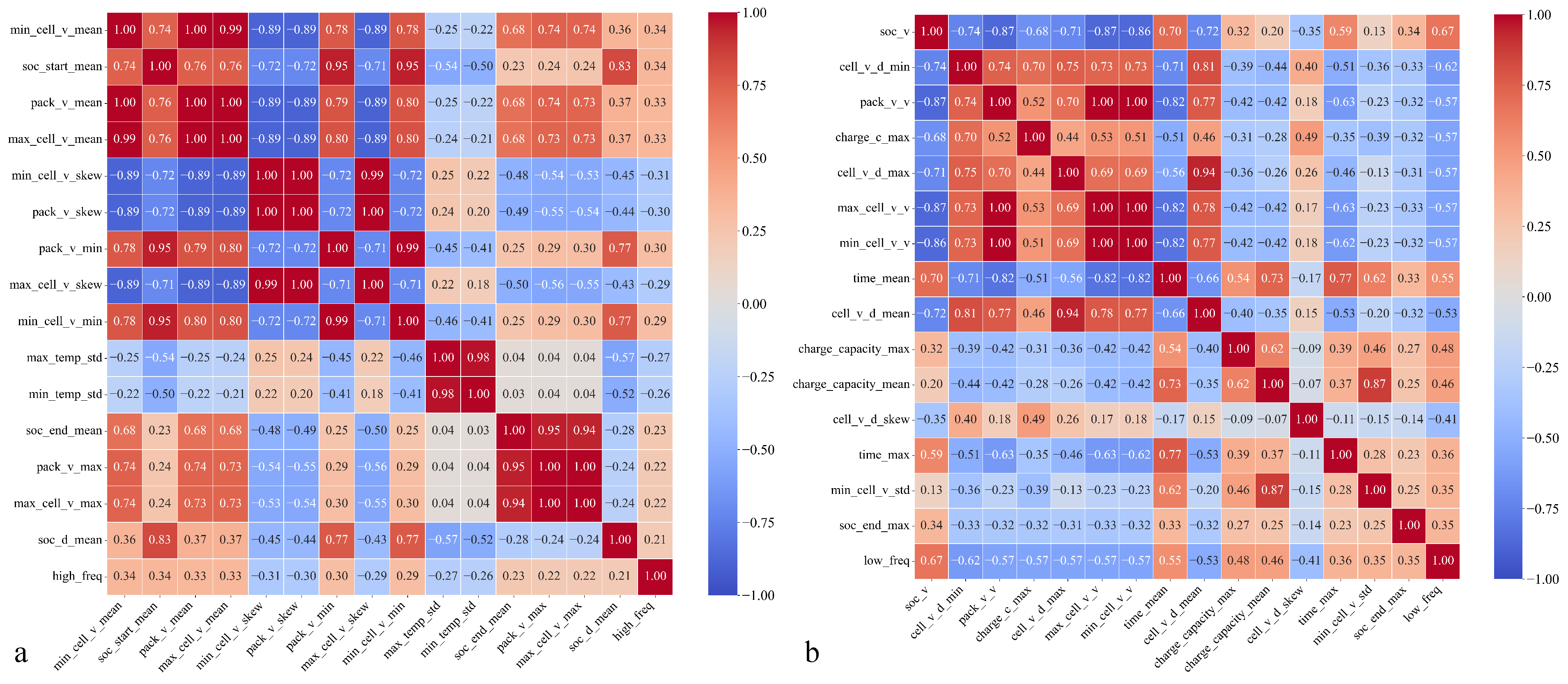
To ensure more accurate and representative correlation analysis between features and capacity while minimizing interference from varying operating environments and conditions across different vehicles, this study calculates Spearman correlation coefficients between features and high/low-frequency capacity components separately for each commercial electric vehicle. The average values across all vehicles are then used as the final evaluation results. A preliminary selection of the top 15 features most correlated with each component is identified as candidate features.

The corresponding high-frequency and low-frequency correlation heatmaps are presented in Figure 6a,b, respectively. From Figure 6a, it can be observed that most features generally exhibit weak correlations with the high-frequency capacity components, showing either low correlation or no clear pattern. This may be attributed to the high-frequency components themselves representing more volatile short-term fluctuations that are susceptible to local anomalies or noise interference. In contrast, Figure 6b reveals that more features demonstrate moderate to strong correlations with the low-frequency capacity components. This aligns well with the fact that low-frequency components reflect the long-term degradation trend of capacity, validating our design approach during the feature extraction phase.

Furthermore, the heatmap reveals that certain feature pairs exhibit perfect correlation ($\rho =1$), such as pack_v_v, max_cell_v_v, and min_cell_v_v, indicating that these features share identical ranking relationships. When such perfectly correlated features are simultaneously used as model inputs, they introduce redundant information and may interfere with effective feature weighting during training, while also increasing computational burden. To address this issue, a correlation-based feature pruning strategy is adopted. Specifically, for each group of perfectly correlated features, only the feature that exhibits the highest correlation with the target capacity sequence is retained, while the remaining features in the same group are removed. In this way, redundant features are eliminated without loss of capacity-relevant information.

The resulting feature sets for high-frequency and low-frequency modeling are summarized in

Table 2. Spearman correlation coefficients of selected features for high-frequency and low-frequency components.

Component	Feature 1	${\mathit{\rho }}_1$	Feature 2	${\mathit{\rho }}_2$
High-frequency	min_cell_v_mean	0.337	soc_start_mean	0.336
	min_cell_v_skew	−0.308	max_temp_std	−0.269
	soc_end_mean	0.226	soc_d_mean	0.210
Low-frequency	soc_v	0.669	cell_v_d_min	−0.618
	pack_v_v	−0.573	charge_c_max	−0.569
	cell_v_d_max	−0.569	time_mean	0.548
	charge_capacity_max	0.481	charge_capacity_mean	0.462
	cell_v_d_skew	−0.413	time_max	0.360
	min_cell_v_std	0.352

. This selection process ensures that each retained feature contributes distinct and relevant information, thereby improving model efficiency and training stability.

4. Methodology

4.1. Overall Framework

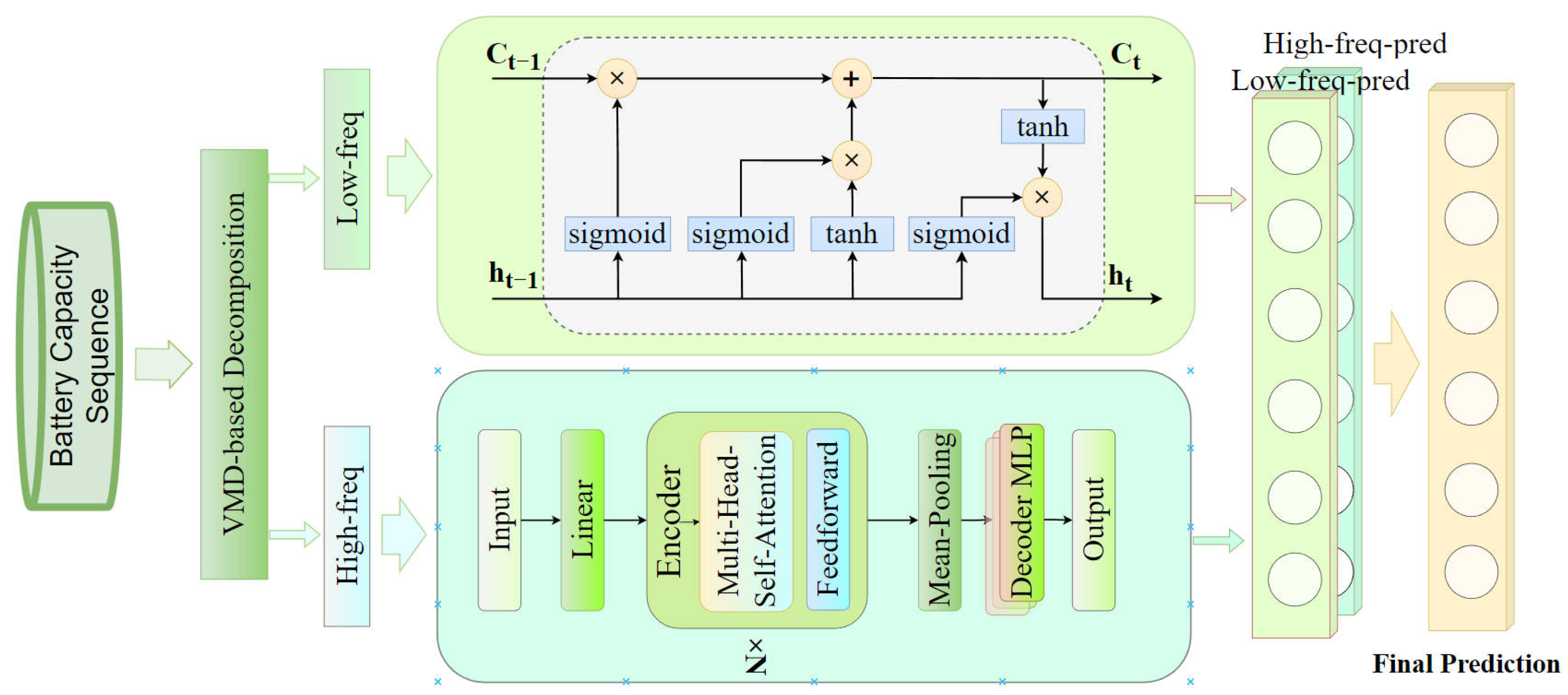
The overall architecture of the hybrid model proposed in this study is illustrated in Figure 7. It consists of two main modules: capacity sequence decomposition and hybrid model prediction. Specifically, the raw capacity sequence is first decomposed into multiple IMFs using VMD. These IMFs are then classified into high-frequency and low-frequency components based on their frequency centroids.

To capture the distinct temporal characteristics across different frequency bands, structurally heterogeneous models are employed: a Transformer for Time Series (TTS) is used to model the high-frequency components, while a Long Short-Term Memory (LSTM) network is applied to the low-frequency components. The final capacity degradation prediction is obtained by integrating the outputs of both models, resulting in a complete and refined estimation of the battery pack’s degradation trajectory.

4.2. Variational Mode Decomposition

The capacity degradation process of battery packs is governed by multiple coupled factors. These include not only intrinsic aging mechanisms but also external and internal interferences such as operating conditions, usage patterns, and cell-to-cell variability. As a result, capacity evolution exhibits both long-term monotonic degradation and short-term irregular fluctuations. Accurately capturing these heterogeneous temporal characteristics is a prerequisite for reliable capacity modeling and long-horizon prediction. To address this requirement, this study adopts VMD to perform multi-scale decomposition of the capacity sequence. Unlike conventional EMD, which relies on recursive sifting and is prone to mode mixing and boundary effects, VMD formulates the decomposition process as a constrained variational optimization problem. This formulation enables the extraction of band-limited intrinsic mode functions with well-defined frequency characteristics. Consequently, VMD provides improved decomposition stability, frequency separability, and robustness when applied to noisy and non-stationary capacity data derived from real-world electric vehicle operation.

The core concept of VMD is to decompose the capacity degradation sequence $x\left(t\right)$ into K intrinsic mode components with limited bandwidth, ensuring each mode exhibits strong spectral compactness in the frequency domain. The fundamental approach involves formulating a variational optimization problem in the frequency domain with the objective of bandwidth minimization, which can be mathematically expressed as follows in Equation (3):

$$\underset{\left\{u_k\right\},\left\{{\omega }_k\right\}}{min}\sum _{k=1}^K{∥{\partial }_t\left[\left(\delta \left(t\right)+{\displaystyle \frac{j}{\pi t}}\right)\ast u_k\left(t\right)\right]e^{-j{\omega }_{k}t}∥}_2^2$$

(3)

The aforementioned optimization problem is subject to the constraints given in Equation (4):

$$\sum _{k=1}^K{u}_k\left(t\right)=x\left(t\right)$$

(4)

where $x\left(t\right)$ denotes the original input signal, $u_k\left(t\right)$ is the k-th decomposed signal, K is the total number of modes, ${\omega }_k$ is the center frequency of the k-th mode, $\delta \left(t\right)$ represents the Dirac delta function, ${\partial }_t$ is the gradient with respect to time t, and j is the imaginary unit.

To solve this constrained variational problem, VMD introduces Lagrangian multipliers and employs the Alternating Direction Method of Multipliers (ADMM) to transform it into an unconstrained optimization problem. The frequency-domain iterative update process consists of three key steps:

• Frequency-domain update of mode components. Each mode component ${\widehat{u}}_k\left(\omega \right)$ is updated in the frequency domain to optimize its compactness around its center frequency, as shown in Equation (5):

  $${\widehat{u}}_k^{n+1}\left(\omega \right)={\displaystyle \frac{\widehat{x}\left(\omega \right)-{\sum }_{i\ne k}{\widehat{u}}_i^n\left(\omega \right)+\frac{{\widehat{\lambda }}^n\left(\omega \right)}{2}}{1+2\alpha {(\omega -{\omega }_k^n)}^2}}$$

  (5)

  where ${\widehat{u}}_k^{n+1}\left(\omega \right)$ is the $(n+1)$-th iteration of the k-th mode in the frequency domain, $\widehat{x}\left(\omega \right)$ is the Fourier transform of the original signal, ${\widehat{u}}_i^n\left(\omega \right)$ is the n-th estimate of the i-th mode ($i\ne k$), ${\widehat{\lambda }}^n\left(\omega \right)$ is the Lagrangian multiplier in the frequency domain, $\omega$ is the angular frequency, ${\omega }_k^n$ is the center frequency of the k-th mode at iteration n, and $\alpha$ is the penalty parameter.
• Update of center frequencies. The center frequencies ${\omega }_k$ are recalculated as the energy-weighted mean frequencies of the mode spectra, which accurately reflects the dominant frequency location of each mode component, according to Equation (6):

  $${\omega }_k^{n+1}={\displaystyle \frac{{\int }_0^{\infty }\omega {\left|{\widehat{u}}_k^{n+1}\left(\omega \right)\right|}^{2}d\omega }{{\int }_0^{\infty }{\left|{\widehat{u}}_k^{n+1}\left(\omega \right)\right|}^{2}d\omega }}$$

  (6)

  where ${\omega }_k^{n+1}$ is the updated center frequency of the k-th mode, and $|{\widehat{u}}_k^{n+1}{\left(\omega \right)|}^2$ represents the spectral energy of the k-th mode at iteration $n+1$.
• Update of Lagrangian multipliers. The multipliers $\widehat{\lambda }\left(\omega \right)$ are adjusted to measure the current reconstruction error between the aggregated modes and the original signal, guiding the decomposition towards the true signal, as defined in Equation (7):

  $${\widehat{\lambda }}^{n+1}\left(\omega \right)={\widehat{\lambda }}^n\left(\omega \right)+\tau \left(\widehat{x}\left(\omega \right)-\sum _{k=1}^K{\widehat{u}}_k^{n+1}\left(\omega \right)\right)$$

  (7)

  where ${\widehat{\lambda }}^{n+1}\left(\omega \right)$ is the updated Lagrange multiplier in the frequency domain, $\tau$ is the dual ascent step size, and K is the total number of modes.

These three steps iterate until mode convergence is achieved, completing the multi-modal decomposition of the capacity sequence. To classify the decomposed modes, we calculate the frequency centroid (see Equation (8)) for each intrinsic mode function (IMF). Modes with frequency centroids ≥0.05 are categorized as high-frequency components, while those with frequency centroids <0.05 are classified as low-frequency components. The respective components within each category are then aggregated through superposition, ultimately yielding the two target constituent signals: the combined high-frequency component and the combined low-frequency component.

$$f_c={\displaystyle \frac{{\sum }_{k=0}^{N/2}{f}_k·\left|X\left(k\right)\right|}{{\sum }_{k=0}^{N/2}\left|X\left(k\right)\right|}}$$

(8)

where $f_c$ denotes the frequency centroid of a signal, $f_k$ is the k-th frequency bin, $\left|X\right(k\left)\right|$ is the amplitude of the k-th bin in the Fourier spectrum, and N is the total number of frequency points.

In this study, the decomposed IMFs are aggregated based on their intrinsic frequency characteristics to distinguish between long-term and short-term components of the capacity sequence. This frequency-domain aggregation provides a compact representation of capacity evolution while preserving its essential temporal structures. The high-frequency components describe short-term variations in the capacity sequence, reflecting rapid changes induced by operating condition fluctuations, measurement uncertainty, and reversible electrochemical effects such as apparent capacity regeneration. These components capture irregular and transient behaviors over short time scales. In contrast, the low-frequency components characterize the smooth and slowly evolving trend of battery capacity over extended time scales. This long-term behavior reflects the cumulative influence of irreversible degradation processes, including active lithium loss, impedance growth, and material degradation, and represents the dominant trajectory of capacity aging.

4.3. TTS–LSTM Hybrid Model

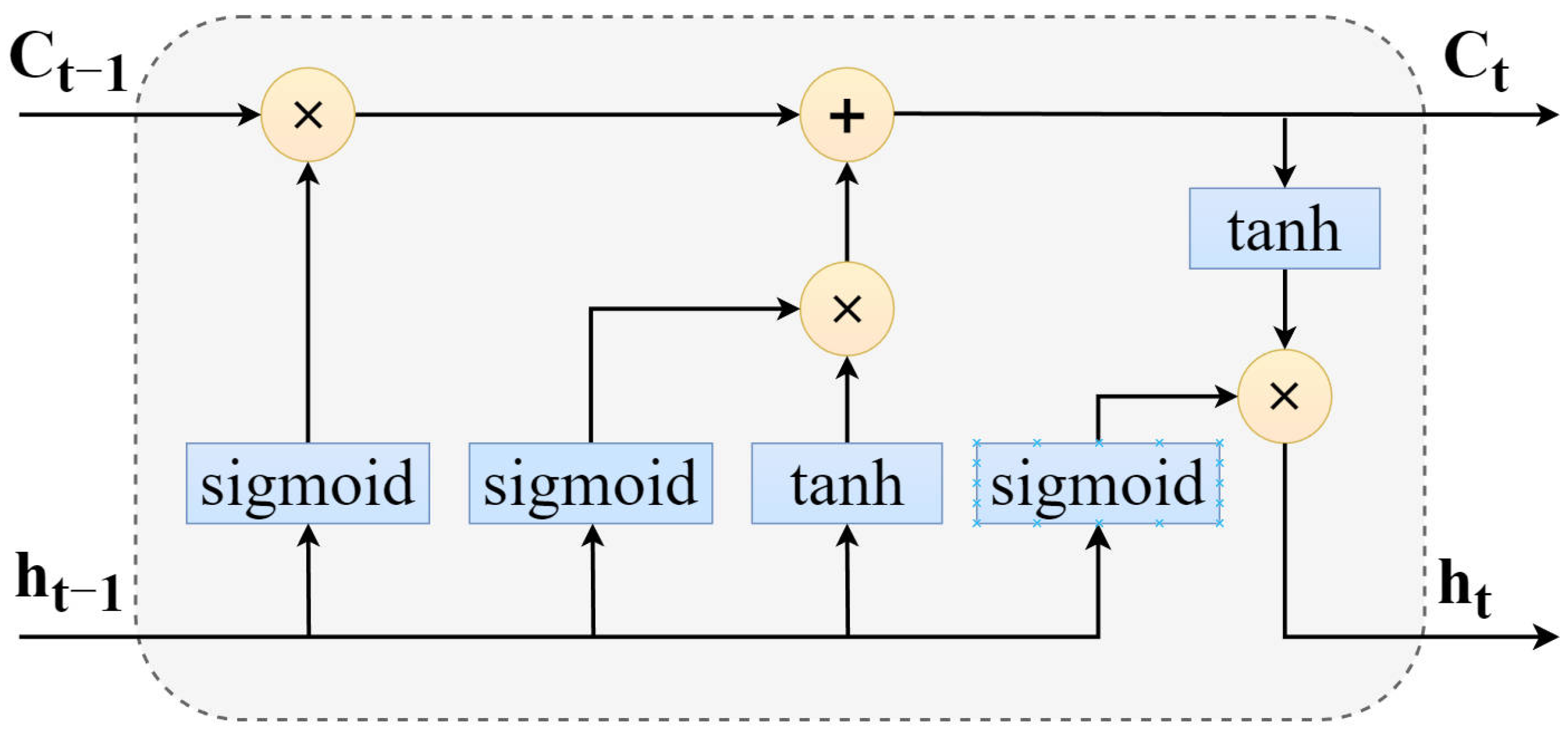
To accurately model the complex battery capacity degradation process that simultaneously exhibits long-term gradual decline trends and short-term fluctuation patterns, this paper proposes a heterogeneous modeling strategy based on high–low frequency decomposition—the TTS–LSTM model. The core idea is to exploit the complementary modeling strengths of different sequence models by assigning them to frequency components with distinct temporal characteristics. Specifically, low-frequency capacity evolution is dominated by smooth and slowly varying trends, whereas high-frequency components mainly reflect short-term fluctuations, operational disturbances, and local irregularities. These two components impose different requirements on temporal modeling. As a classic variant of recurrent neural networks, LSTM employs sophisticated gating mechanisms to dynamically regulate information flow, effectively overcoming the vanishing/exploding gradient problems inherent in traditional RNNs. This architecture demonstrates exceptional capability in capturing and maintaining long-term dependencies, making it particularly suitable for modeling the slowly evolving low-frequency trends of battery capacity. Compared to conventional RNNs, LSTM significantly improves training stability and medium-to-long-term prediction accuracy. The detailed cell structure is illustrated in Figure 8.

However, the inherent sequential processing mechanism and relatively localized receptive field of LSTM constrain its effectiveness in capturing rapidly changing patterns, non-local dependencies, and complex global relationships within sequences. These limitations become more pronounced when modeling high-frequency capacity components, which exhibit irregular variations and short-term dependencies across distant time steps. For such components, an efficient mechanism for global dependency modeling without recursive error accumulation is required.

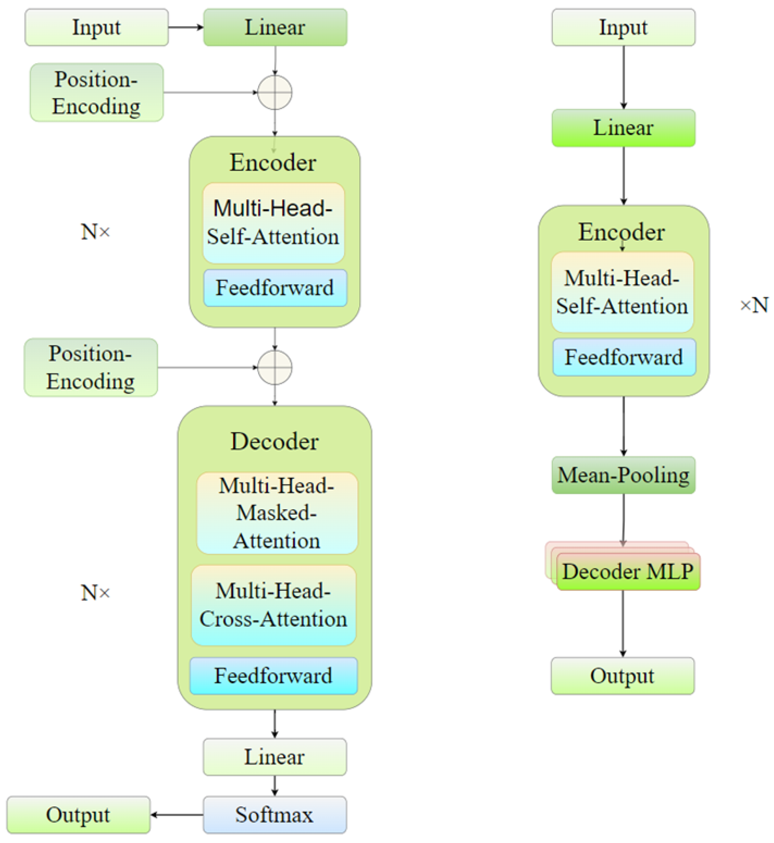
To address this issue, the TTS module is introduced to model the high-frequency components. TTS is derived from the Transformer encoder architecture and is specifically tailored for time series prediction tasks. Its design motivation is to retain the Transformer’s strong global dependency modeling capability while removing structural components that are unnecessary for non-autoregressive capacity degradation prediction.

As illustrated in Figure 9, the left panel displays the standard Transformer structure while the right panel presents the TTS model architecture. Unlike the standard Transformer, TTS employs linear projection to map raw sequences into an embedded space and utilizes stacked multi-head self-attention layers to efficiently capture non-local dependencies across arbitrary time steps and global patterns. The decoder and autoregressive mechanism are removed, and time-dimensional average pooling combined with fully connected layers is adopted for non-autoregressive prediction. These design choices reduce computational complexity, avoid error accumulation in multi-step prediction, and improve robustness under noisy or limited real-world data conditions, while preserving sufficient representational capacity.

5. Experimental Results and Analysis

5.1. Experimental Setup

In real-world electric vehicle applications, battery management systems (BMS) are not primarily concerned with the instantaneous capacity at a single time point, but rather focus on the long-term degradation trend of the battery pack. Moreover, since only current and historical measurements are available in practice, the capacity degradation prediction task addressed in this study is formulated as a multi-feature, multi-step input and multi-step output time series forecasting problem. The corresponding input–output structure is illustrated in Equation (9).

$$D=[\mathrm{Input}\mid \mathrm{Output}]=\left\{\begin{array}{cccccc}{x}_{11}& x_{12}& x_{13}& \cdots & x_{1m}& y_{n+1}\\ x_{21}& x_{22}& x_{23}& \cdots & x_{2m}& y_{n+2}\\ ⋮& ⋮& ⋮& \ddots & ⋮& ⋮\\ x_{n1}& x_{n2}& x_{n3}& \cdots & x_{nm}& y_{n+w}\end{array}\right\}$$

(9)

where y denotes the capacity sequence, $x_i$ represents the i-th input feature, n is the input sequence length, m is the number of features, and w is the prediction horizon.

In this study, data from Vehicles #1 and #2 are reserved as the prediction set, while the remaining vehicles are used for model training, with each vehicle treated as an independent sample. This setup reflects a common real-world prediction task, where a model trained on multiple vehicles forecasts the degradation of an individual, unseen vehicle from the same city but with distinct usage patterns, thereby testing its practical utility. After data preprocessing and cleaning, each vehicle provides between 120 and 140 valid samples. To avoid potential bias caused by unequal sample sizes, the first 120 samples from each vehicle are uniformly selected. During training, the first 20 capacity points are assumed to be known, and the model is tasked with predicting the subsequent 100-step capacity degradation trajectory.

Based on the above setting, model performance is evaluated on high-frequency components, low-frequency components, and the full-frequency capacity sequence. Accordingly, several representative baseline models are selected for comparison. Specifically, LSTM is adopted as classical recurrent models for temporal dependency modeling. Attention-based models, including Transformer and seq2seq, are employed to capture long-range dependencies. Among them, the seq2seq architecture corresponds to the core predictive model used in the original dataset publication [49]. In addition, TCN is introduced as a representative convolution-based time series model. The TCN represents the main temporal modeling component of convolution-based approaches reported in recent battery degradation studies [46]. Under this experimental setting, the proposed framework is systematically evaluated against the above baseline models to verify its predictive performance and modeling effectiveness. In addition, we repeat the experiments 10 times on the high-frequency, low-frequency, and full-frequency components to check the stability of the proposed framework. We also conduct experiments with different input sequence lengths to see how the prediction performance changes with different amounts of historical data.

5.2. Evaluation Criteria

To comprehensively evaluate the model’s predictive performance and its deviation from actual values, this study employs three established metrics: root mean square error (RMSE), mean absolute error (MAE), and mean absolute percentage error (MAPE), with corresponding formulas provided in Equations (10)–(12). The MAE quantifies the average magnitude of absolute errors between predicted and actual values, measuring the mean deviation level of predictions from ground truth—smaller values indicate higher accuracy. The RMSE assigns greater weight to larger errors during calculation, making it more sensitive to outlier errors than MAE and better reflecting the model’s comprehensive precision. The MAPE calculates prediction errors as percentages relative to actual values and averages these percentages, providing an intuitive representation of relative error levels across different measurement scales or magnitudes.

$$\mathrm{MAE}={\displaystyle \frac{1}{n}}\sum _{i=1}^n|{\widehat{y}}_i-y_i|$$

(10)

$$\mathrm{RMSE}=\sqrt{{\displaystyle \frac{1}{n}}{\displaystyle \sum _{i=1}^n}{({\widehat{y}}_i-y_i)}^2}$$

(11)

$$\mathrm{MAPE}={\displaystyle \frac{100\%}{n}}{\displaystyle \sum _{i=1}^n}\left|{\displaystyle \frac{{\widehat{y}}_i-y_i}{y_i}}\right|$$

(12)

In the above equations, n denotes the total number of prediction samples, ${\widehat{y}}_i$ represents the predicted value at the i-th time step, and $y_i$ is the corresponding actual (ground truth) value.

5.3. Feature Set Validation

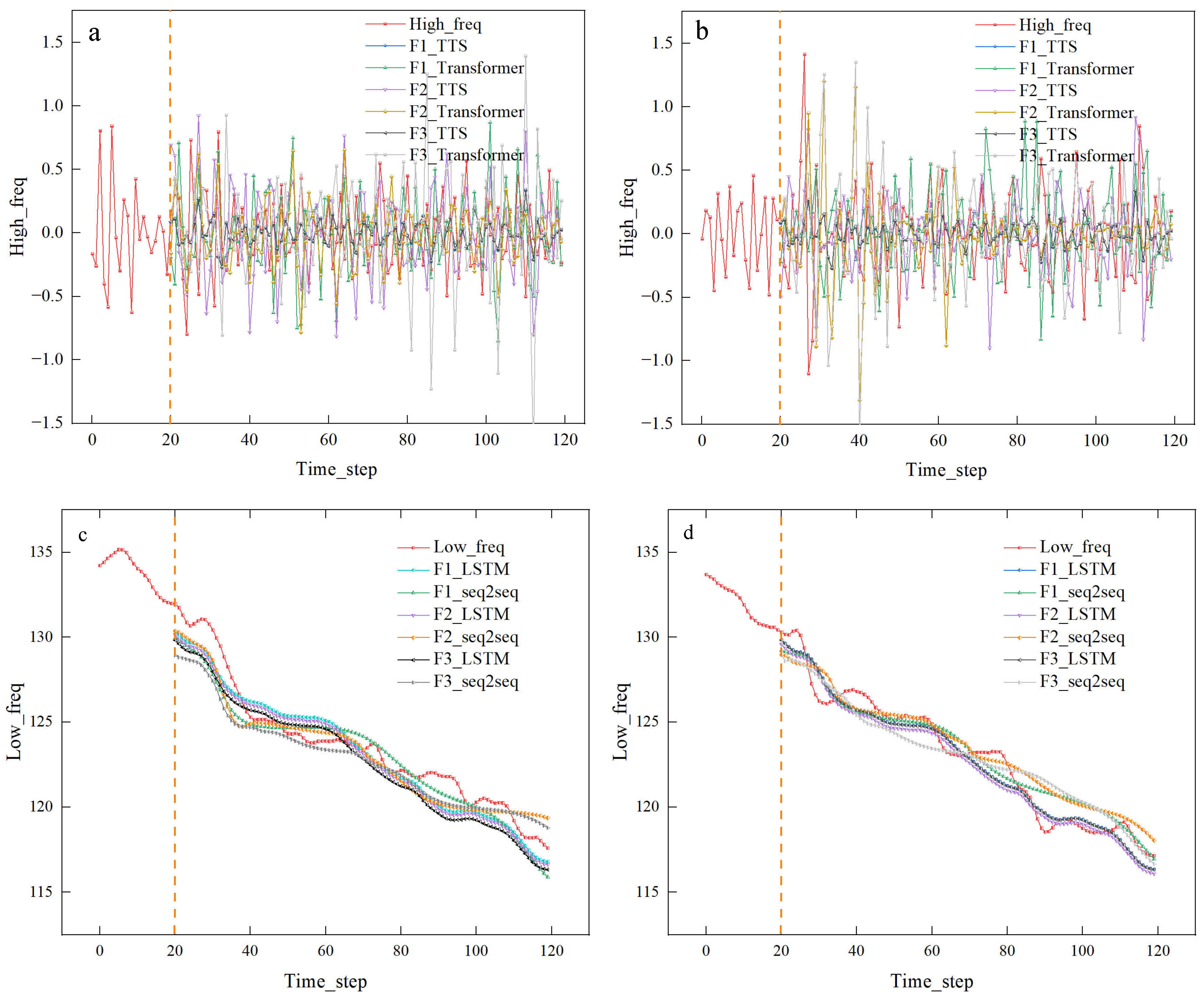
To validate the effectiveness of the proposed feature extraction process, separate models were constructed for the high-frequency and low-frequency components, using three feature sets—F1, F2, and F3—as inputs. Specifically, F1 represents the optimal feature subset determined by the proposed feature selection procedure (as shown in Table 2); F2 consists of the top 15 features ranked by correlation, containing 9 and 3 redundant features compared with F1 in the high- and low-frequency cases, respectively; and F3 comprises all extracted features. The prediction results based on different feature sets are illustrated in Figure 10, while the corresponding evaluation metrics for both frequency components are summarized in

Table 3. Validation results of models with different feature sets.

Feature Set	Component	Model	MAE	RMSE	MAPE (%)
F1	High-frequency	TTS	0.2897	0.3705	1.5680
		Transformer	0.3955	0.4875	20.7804
	Low-frequency	LSTM	0.8119	0.9454	0.0066
		seq2seq	0.8700	1.0650	0.0070
F2	High-frequency	TTS	0.2900	0.3706	1.6542
		Transformer	0.3965	0.5249	9.8293
	Low-frequency	LSTM	0.8954	1.0433	0.0072
		seq2seq	0.9015	1.1907	0.0076
F3	High-frequency	TTS	0.2902	0.3706	1.6226
		Transformer	0.4371	0.5729	4.6737
	Low-frequency	LSTM	0.9186	1.0808	0.0074
		seq2seq	1.0357	1.2915	0.0083

.

The results demonstrate that all three feature sets achieve relatively accurate predictions for both high- and low-frequency components, indicating that the constructed models are capable of effectively capturing the capacity degradation trend. However, F1 consistently achieves the best overall performance, with significantly lower MAE and RMSE values than F2 and F3 across all models. This suggests that the features obtained through the proposed selection process better capture the key patterns of capacity variation, thereby improving the model’s generalization and stability. In contrast, although F2 includes more highly correlated features, the presence of redundant variables may introduce noise or multicollinearity, leading to partial overfitting during training. Similarly, F3 incorporates all features, but the increased dimensionality of the feature space reduces its generalization capability. Overall, the F1 feature set constructed through a well-designed selection strategy exhibits superior prediction accuracy and robustness in both high- and low-frequency modeling, confirming the effectiveness of the proposed feature extraction and selection framework for battery capacity degradation modeling.

5.4. Frequency Division Prediction Results and Analysis

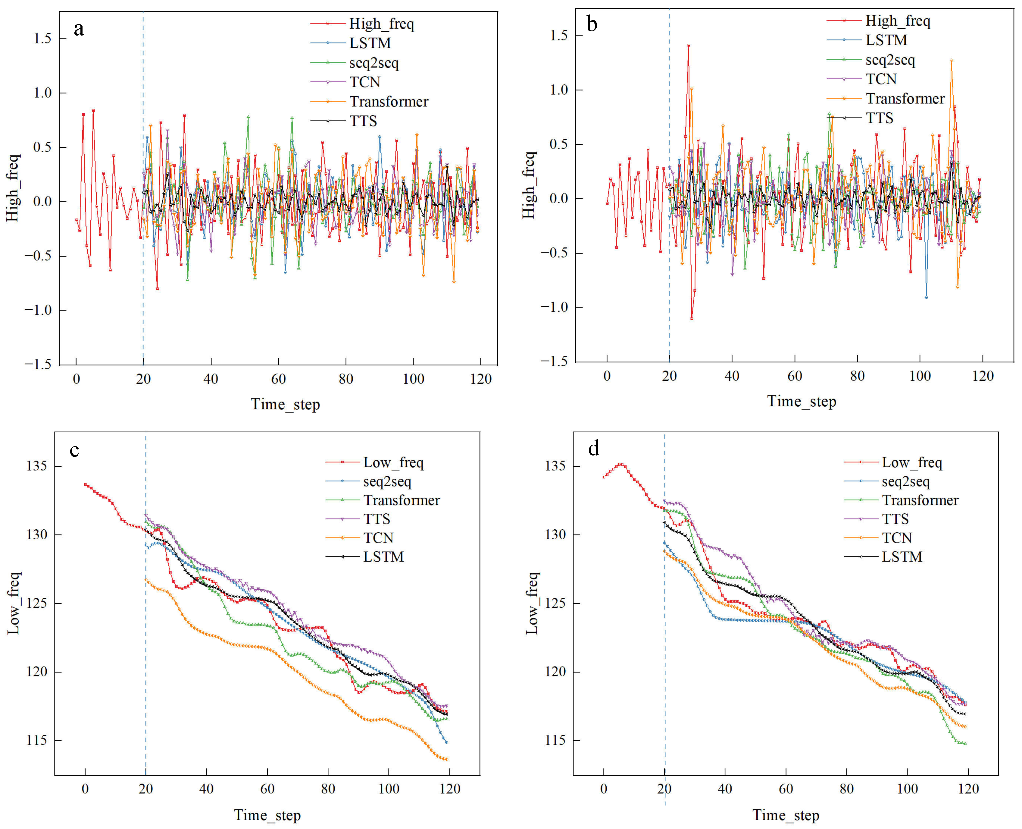
This study decomposes the capacity sequence into high-frequency and low-frequency components for separate modeling. Both components employ identical input–output configurations to ensure design consistency and comparability. Figure 11a,b compare the performance of TTS, LSTM, Seq2Seq, TCN, and standard Transformer models on high-frequency component prediction using features detailed in Table 2. Under the configuration of 20-step input and 100-step output, TTS demonstrates superior convergence and generalization capabilities when handling rapidly fluctuating short-term sequences compared to standard Transformer.

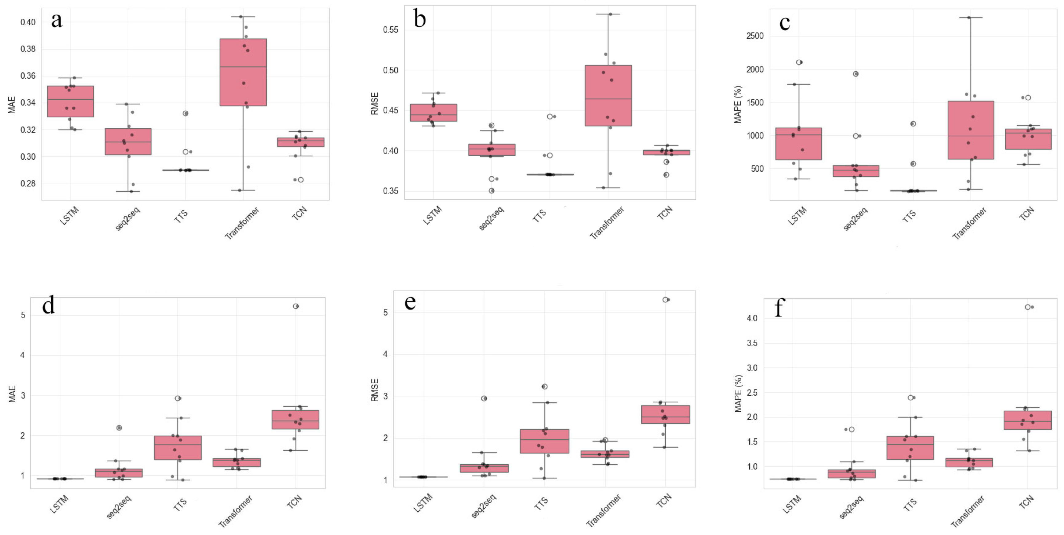
Benefiting from its lightweight design and non-autoregressive prediction mechanism, TTS effectively suppresses noise interference while accurately capturing structural characteristics of high-frequency signals. The statistical results from 10 repeated experiments (

Table 4. Frequency division prediction results for high-frequency and low-frequency components (mean ± std over repeated experiments). The best-performing model under each evaluation metric is highlighted in bold.

Component	Model	MAE	RMSE	MAPE
High-frequency	LSTM	0.3406 ± 0.0135	0.4480 ± 0.0133	10.3179 ± 5.2286
	seq2seq	0.3092 ± 0.0198	0.3985 ± 0.0232	6.1850 ± 4.8419
	TTS	0.2954 ± 0.0129	0.3801 ± 0.0220	3.0718 ± 3.1599
	TCN	0.3084 ± 0.0098	0.3958 ± 0.0099	9.9753 ± 2.7000
	Transformer	0.3550 ± 0.0418	0.4617 ± 0.0638	11.0805 ± 7.2463
Low-frequency	LSTM	0.9186 ± 0.0147	1.0810 ± 0.0139	0.0074 ± 0.0012
	seq2seq	1.1818 ± 0.3605	1.4676 ± 0.5186	0.0095 ± 0.0029
	TTS	1.7579 ± 0.5962	2.0124 ± 0.6325	0.0143 ± 0.0049
	TCN	2.5802 ± 0.9355	2.7300 ± 0.9089	0.0209 ± 0.0076
	Transformer	1.3697 ± 0.1667	1.6377 ± 0.1818	0.0111 ± 0.0014

) show that TTS achieves an average MAE of 0.2954 ± 0.0129, RMSE of 0.3801 ± 0.0220, and MAPE of 3.0718 ± 3.1599, significantly outperforming other models. The error distributions for high-frequency components (Figure 12a–c) further illustrate the stability of TTS, with compact boxes indicating consistent performance across repeated runs. Figure 11c,d present outcomes of TCN, LSTM, Seq2Seq, and Transformer models on low-frequency component prediction. The LSTM model excels in capturing long-term gradual degradation trends, yielding smoother and better-aligned predictions. As quantified in Table 4, LSTM achieves an average MAE of 0.9186 ± 0.0147, RMSE of 1.0810 ± 0.0139, and MAPE of 0.0074 ± 0.0012, demonstrating superior trend modeling capabilities over baseline models. The exceptionally narrow error distributions for LSTM on low-frequency components (Figure 12d–f) confirm its remarkable stability and reproducibility.

The results reveal a complementary relationship between TTS and LSTM: each excels at modeling a distinct part of the signal. TTS performs best on the high-frequency component (MAE: 0.2954), which is dominated by short-term fluctuations and noise. In contrast, LSTM achieves the highest accuracy on the low-frequency component (MAE: 0.9186), which represents the underlying long-term degradation trend. This clear specialization—TTS for fast-varying details and LSTM for slow-varying trends—directly supports our core strategy of building a hybrid model that combines their strengths to capture the full complexity of battery capacity decay.

5.5. Integrated Prediction Results

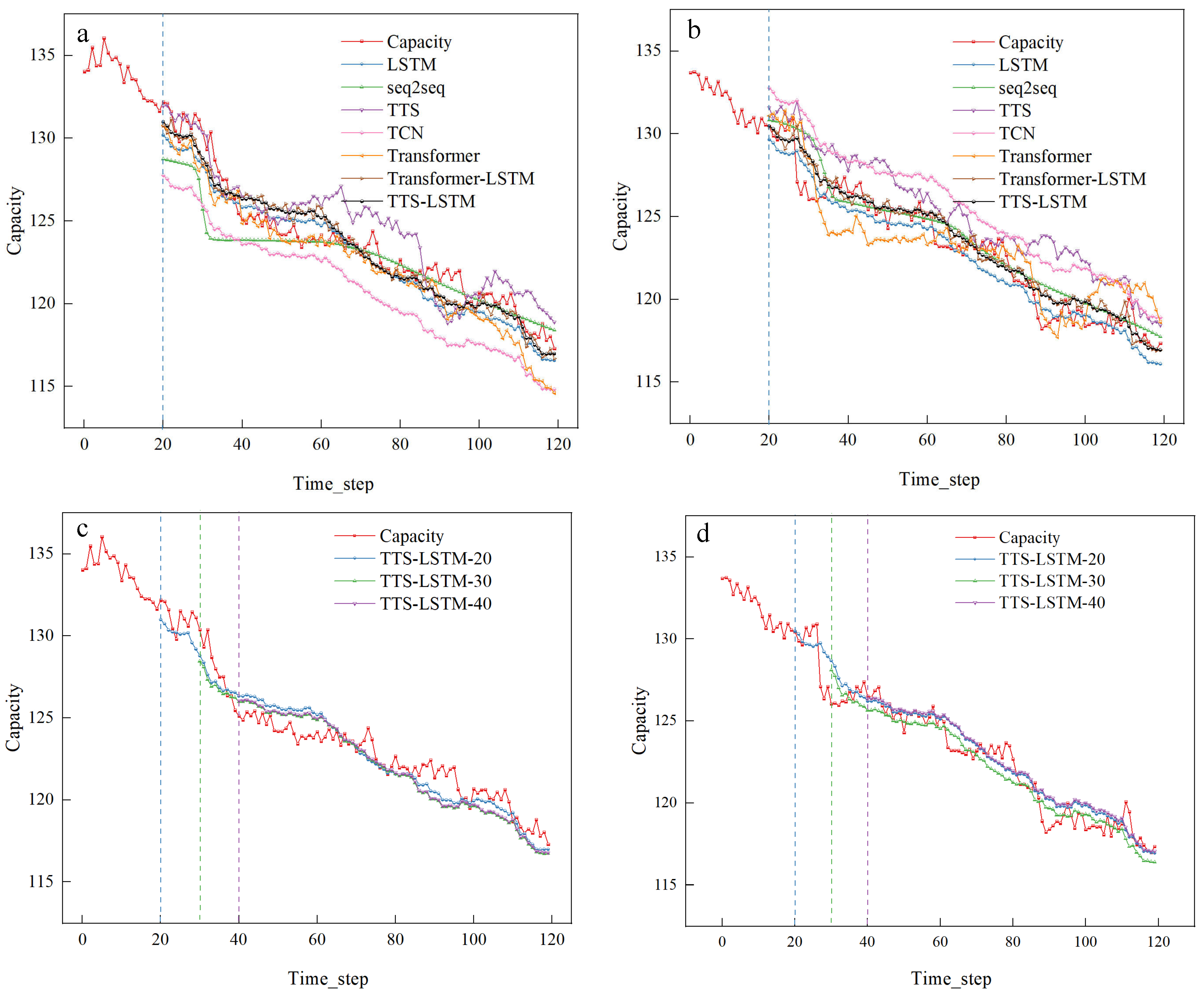
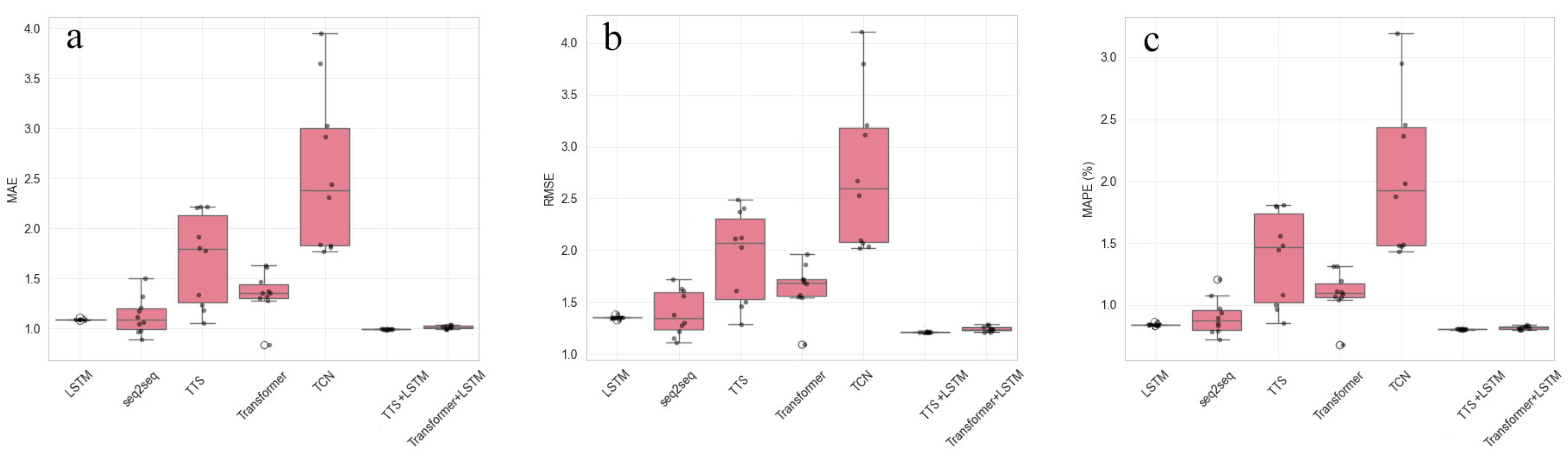
Through the aforementioned comparative experiments, we have validated the applicability of different models in processing capacity signals at varying frequencies: TTS demonstrates superior stability and fitting capability for modeling high-frequency fluctuations, while LSTM excels at capturing low-frequency trend variations, enabling more effective characterization of the long-term degradation process in battery pack capacity. Building upon this foundation, our integrated model adopts these two complementary architectures to construct a heterogeneous framework specifically designed for high- and low-frequency components, fusing their predictions to generate the final capacity degradation prediction curve. For model validation, we compare the integrated model’s predictions against the undivided true capacity sequences while introducing baseline models including the original Transformer, LSTM, TCN, Seq2Seq, and a Transformer–LSTM integrated model—all trained under identical feature selection conditions on undivided data as controls. Figure 13a,b illustrates prediction results for Vehicles #1 and #2. The integrated model, owing to its frequency-decomposed structure aligning with the multi-scale nature of capacity degradation, produces fused results that smoothly track the overall degradation trend while preserving essential local fluctuations, demonstrating enhanced robustness and stability across both samples.

Table 5. Prediction error metrics of the ensemble model vs. baseline models (mean ± std over repeated experiments). The best-performing model under each evaluation metric is highlighted in bold.

Model	MAE	RMSE	MAPE (%)
LSTM	0.9929 ± 0.0115	1.2130 ± 0.0124	0.0080 ± 0.0032
seq2seq	1.1239 ± 0.1731	1.3963 ± 0.2060	0.0091 ± 0.0014
TTS	1.6946 ± 0.4351	1.9384 ± 0.4147	0.0138 ± 0.0035
Transformer	1.3515 ± 0.2076	1.6395 ± 0.2207	0.0110 ± 0.0017
TTS–LSTM	0.9247 ± 0.0055	1.0151 ± 0.0079	0.0074 ± 0.0009
Transformer–LSTM	1.0115 ± 0.0159	1.2436 ± 0.0244	0.0082 ± 0.0001

summarizes average prediction metrics across models based on 10 repeated experiments. TTS–LSTM achieves MAE = 0.9247 ± 0.0055, RMSE = 1.0151 ± 0.0079, and MAPE = 0.0074 ± 0.0009, significantly outperforming undivided models like LSTM (MAE = 0.9929 ± 0.0115, RMSE = 1.2130 ± 0.0124, MAPE = 0.0080 ± 0.0032) and Transformer (MAE = 1.3515 ± 0.2076, RMSE = 1.6395 ± 0.2207, MAPE = 0.0110 ± 0.0017). Compared to LSTM applied directly to raw capacity sequences, TTS–LSTM reduces MAE by 0.0682, RMSE by 0.1979, and MAPE by 0.0006. Against the standard Transformer–LSTM architecture (MAE = 1.0115 ± 0.0159, RMSE = 1.2436 ± 0.0244, MAPE = 0.0082 ± 0.0001), TTS–LSTM further reduces MAE by 0.0868, RMSE by 0.2285, and MAPE by 0.0008. The error distribution analysis in Figure 14 provides further insights into model stability. The box plots for LSTM show exceptionally narrow distributions (MAE: 0.9929 ± 0.0115, RMSE: 1.2130 ± 0.0124), indicating high consistency across repeated runs. In contrast, Transformer and TTS exhibit wider error distributions, particularly in MAPE (TTS: 0.0138 ± 0.0035%, Transformer: 0.0110 ± 0.0017%), suggesting higher variability. Notably, TTS–LSTM demonstrates both competitive performance and good stability, with relatively compact error distributions (MAE: 0.9247 ± 0.0055) that bridge the gap between the stability of LSTM and the modeling capacity of Transformer-based architectures.

These results confirm that both integrated frameworks substantially outperform undivided strategies across all metrics, validating the efficacy of our heterogeneous integration approach based on frequency decoupling and component-specific analysis for improving prediction accuracy. Moreover, TTS–LSTM’s marked advantages over Transformer–LSTM comprehensively demonstrate TTS’s superiority in high-frequency modeling.

5.6. Predictions from Different Starting Points

This section evaluates the proposed integrated model’s performance in predicting future battery pack capacity trajectories from different starting points. Figure 13c,d displays prediction results for Vehicles #1 and #2 using input lengths of 20, 30, and 40 steps to forecast future capacities over 100, 90, and 80 steps, respectively.

Table 6. Prediction results from different starting points.

Input and Output Steps	MAE	RMSE	MAPE (%)
(20, 100)	0.8874	1.0581	0.0069
(30, 90)	0.8470	1.0401	0.0062
(40, 80)	0.8234	1.0126	0.0054

lists the model’s average prediction error metrics under these configurations. The data reveals that with a (20, 100) step configuration, the model achieves MAE = 0.8874 and RMSE = 1.0581. Prediction errors gradually decrease with longer input sequences: Under (30, 90) and (40, 80) configurations, MAE drops to 0.8470 and 0.8234, RMSE reduces to 1.0401 and 1.0126, while MAPE decreases to 0.0062 and 0.0054.

This accuracy improvement fundamentally stems from extended battery usage duration providing richer historical degradation patterns. As operational time accumulates, the model captures more complete aging signatures—including nonlinear decay phases and recovery effects—thereby enhancing prediction reliability. Notably, shorter input sequences offer advantages in real-time responsiveness but sacrifice some aging context. The observed performance trade-off reflects an essential engineering principle: extended service time generates more representative degradation data, enabling models to establish robust capacity trajectory projections. Practical deployment should balance data completeness against system constraints.

6. Conclusions

This study proposes a hybrid VMD–TTS–LSTM framework for long-term battery capacity prediction using real-world electric vehicle charging data. The framework integrates Variational Mode Decomposition with a heterogeneous modeling strategy to effectively decouple and represent the multi-scale degradation characteristics of batteries. Results from ten repeated experiments show that under the configuration of 20-step input and 100-step output, the proposed method achieves a mean absolute error of 0.9247 ± 0.0055 and a root mean square error of 1.0151 ± 0.0079. These findings confirm the model’s robustness and predictive accuracy, demonstrating its superior performance over several established baseline models. The study indicates that reliable long-term capacity estimation can be achieved using routine charging data alone. This outcome offers a practical, data-driven solution for battery health monitoring in electric vehicles. It should be noted that the current validation is based on data from electric taxis operating within the same city. Future work will extend the framework to more diverse operating environments and integrate multi-source information—such as thermal and electrochemical signals—to further enhance its generalization capability and practical applicability. In addition, the sensitivity and optimization of several empirically set parameters in this study warrant further investigation.

References

1. Igliński, B.; Kiełkowska, U.; Pietrzak, M.B.; Skrzatek, M.; Kumar, G.; Piechota, G. The regional energy transformation in the context of renewable energy sources potential. Renew. Energy 2023, 218, 119246. [Google Scholar] [CrossRef]
2. Manfo, T.A. A Comprehensive Analysis of Material Revolution to Evolution in Lithium-ion Battery Technology. Turk. J. Mater. 2023, 8, 1–13. [Google Scholar]
3. He, Z.; Wang, H.; Xiang, J.; Chen, C. Enhancing the Sustainability of Underground Battery Storage: A Robust SOC Estimation Model Against Thermal Variations for Green Energy Systems. J. Geo-Energy Environ. 2025, 1, 88–95. [Google Scholar] [CrossRef]
4. Xiang, J.; He, Z.; Lei, G.; Chen, C. Life Cycle Assessment of Iridium Production: Environmental Impact Analysis Based on Brightway2. J. Geo-Energy Environ. 2025, 1, 70–75. [Google Scholar] [CrossRef]
5. Demirci, O. Review of battery state estimation methods for electric vehicles-part II: SOH estimation. J. Energy Storage 2024, 96, 112703. [Google Scholar] [CrossRef]
6. Rodriguez-Cea, A.I.; Morinigo-Sotelo, D.; Tinaut, F.V. A procedure for evaluating the SOH of Li-ion batteries from data during the constant voltage charge phase and the use of an ECM with internal resistance. J. Energy Storage 2025, 108, 115074. [Google Scholar] [CrossRef]
7. Sihvo, J.; Roinila, T.; Stroe, D.-I. SOH analysis of Li-ion battery based on ECM parameters and broadband impedance measurements. In Proceedings of the IECON 2020 The 46th Annual Conference of the IEEE Industrial Electronics Society, Singapore, 18–21 October 2020; pp. 1923–1928. [Google Scholar]
8. Li, C.; Yang, L.; Li, Q.; Zhang, Q.; Zhou, Z.; Meng, Y.; Zhao, X.; Wang, L.; Zhang, S.; Li, Y.; et al. SOH estimation method for lithium-ion batteries based on an improved equivalent circuit model via electrochemical impedance spectroscopy. J. Energy Storage 2024, 86, 111167. [Google Scholar] [CrossRef]
9. Vennam, G.; Sahoo, A. A dynamic SOH-coupled lithium-ion cell model for state and parameter estimation. IEEE Trans. Energy Convers. 2023, 38, 1186–1196. [Google Scholar] [CrossRef]
10. Hu, C.; Youn, B.D.; Chung, J. A multiscale framework with extended kalman filter for lithium-ion battery SOC and capacity estimation. Appl. Energy 2012, 92, 694–704. [Google Scholar] [CrossRef]
11. Azis, N.A.; Joelianto, E.; Widyotriatmo, A. State of charge (SoC) and state of health (SoH) estimation of lithium-ion battery using dual extended kalman filter based on polynomial battery model. In Proceedings of the 2019 6th International Conference on Instrumentation, Control, and Automation (ICA), Bandung, Indonesia, 31 July–2 August 2019; pp. 88–93. [Google Scholar]
12. Merla, Y.; Wu, B.; Yufit, V.; Martinez-Botas, R.F.; Offer, G.J. An easy-to-parameterise physics-informed battery model and its application towards lithium-ion battery cell design, diagnosis, and degradation. J. Power Sources 2018, 384, 66–79. [Google Scholar] [CrossRef]
13. Kim, J.; Chun, H.; Kim, M.; Han, S.; Lee, J.-W.; Lee, T.-K. Effective and practical parameters of electrochemical li-ion battery models for degradation diagnosis. J. Energy Storage 2021, 42, 103077. [Google Scholar] [CrossRef]
14. Hosseininasab, S.; Lin, C.; Pischinger, S.; Stapelbroek, M.; Vagnoni, G. State-of-health estimation of lithium-ion batteries for electrified vehicles using a reduced-order electrochemical model. J. Energy Storage 2022, 52, 104684. [Google Scholar] [CrossRef]
15. Jiang, B.; Dai, H.; Wei, X. Incremental capacity analysis based adaptive capacity estimation for lithium-ion battery considering charging condition. Appl. Energy 2020, 269, 115074. [Google Scholar] [CrossRef]
16. Sun, H.; Yang, D.; Wang, L.; Wang, K. A method for estimating the aging state of lithium-ion batteries based on a multi-linear integrated model. Int. J. Energy Res. 2022, 46, 24091–24104. [Google Scholar] [CrossRef]
17. Liu, G.; Ouyang, M.; Lu, L.; Li, J.; Han, X. Online estimation of lithium-ion battery remaining discharge capacity through differential voltage analysis. J. Power Sources 2015, 274, 971–989. [Google Scholar] [CrossRef]
18. Zheng, L.; Zhu, J.; Wang, G.; Lu, D.D.-C.; He, T. Differential voltage analysis based state of charge estimation methods for lithium-ion batteries using extended kalman filter and particle filter. Energy 2018, 158, 1028–1037. [Google Scholar] [CrossRef]
19. Li, H.; Chen, C. Lithium-ion battery SOH prediction based on multi-dimensional features and multi-model feature selector. Energy 2025, 331, 136844. [Google Scholar] [CrossRef]
20. Lin, C.; Xu, J.; Shi, M.; Mei, X. Constant current charging time based fast state-of-health estimation for lithium-ion batteries. Energy 2022, 247, 123556. [Google Scholar] [CrossRef]
21. Li, Q.; Li, D.; Zhao, K.; Wang, L.; Wang, K. State of health estimation of lithium-ion battery based on improved ant lion optimization and support vector regression. J. Energy Storage 2022, 50, 104215. [Google Scholar] [CrossRef]
22. Tong, L.; Gong, M.; Chen, Y.; Kuang, R.; Xu, Y.; Zhang, H.; Peng, B.; Yang, F.; Zhang, J.; Li, Y. State of health estimation of lithium-ion battery for electric vehicle based on VMD-DBO-SVR model. J. Electrochem. Soc. 2024, 171, 080504. [Google Scholar] [CrossRef]
23. Guo, Y.; Huang, K.; Yu, X.; Wang, Y. State-of-health estimation for lithium-ion batteries based on historical dependency of charging data and ensemble SVR. Electrochim. Acta 2022, 428, 140940. [Google Scholar] [CrossRef]
24. Yang, D.; Wang, Y.; Pan, R.; Chen, R.; Chen, Z. State-of-health estimation for the lithium-ion battery based on support vector regression. Appl. Energy 2018, 227, 273–283. [Google Scholar] [CrossRef]
25. Yan, N.; Yao, Y.-B.; Jia, Z.-D.; Liu, L.; Dai, C.-T.; Li, Z.-G.; Zhang, Z.-H.; Li, W.; Wang, L.; Wang, P.-F. Online battery health diagnosis for electric vehicles based on DTW-XGBoost. Energy Rep. 2022, 8, 121–128. [Google Scholar] [CrossRef]
26. Deng, Z.; Hu, X.; Li, P.; Lin, X.; Bian, X. Data-driven battery state of health estimation based on random partial charging data. IEEE Trans. Power Electron. 2022, 37, 5021–5031. [Google Scholar] [CrossRef]
27. Xiong, X.; Wang, Y.; Li, K.; Chen, Z. State of health estimation for lithium-ion batteries using gaussian process regression-based data reconstruction method during random charging process. J. Energy Storage 2023, 72, 108390. [Google Scholar] [CrossRef]
28. Li, P.; Zhang, Z.; Xiong, Q.; Ding, B.; Hou, J.; Luo, D.; Rong, Y.; Li, S. State-of-health estimation and remaining useful life prediction for the lithium-ion battery based on a variant long short term memory neural network. J. Power Sources 2020, 459, 228069. [Google Scholar] [CrossRef]
29. Zhang, N.; Li, J.; Ma, Y.; Wu, K. Lithium-Ion batteries state of health estimation based on optimized TCN-GRU-WNN. Energy Rep. 2025, 13, 2502–2515. [Google Scholar] [CrossRef]
30. Peng, S.; Sun, Y.; Liu, D.; Yu, Q.; Kan, J.; Pecht, M. State of health estimation of lithium-ion batteries based on multi-health features extraction and improved long short-term memory neural network. Energy 2023, 282, 128956. [Google Scholar] [CrossRef]
31. Ma, Y.; Shan, C.; Gao, J.; Chen, H. A novel method for state of health estimation of lithium-ion batteries based on improved LSTM and health indicators extraction. Energy 2022, 251, 123973. [Google Scholar] [CrossRef]
32. Zhao, H.; Chen, Z.; Shu, X.; Shen, J.; Lei, Z.; Zhang, Y. State of health estimation for lithium-ion batteries based on hybrid attention and deep learning. Reliab. Eng. Syst. Saf. 2023, 232, 109066. [Google Scholar] [CrossRef]
33. Fan, Y.; Xiao, F.; Li, C.; Yang, G.; Tang, X. A novel deep learning framework for state of health estimation of lithium-ion battery. J. Energy Storage 2020, 32, 101741. [Google Scholar] [CrossRef]
34. Xu, H.; Wu, L.; Xiong, S.; Li, W.; Garg, A.; Gao, L. An improved CNN-LSTM model-based state-of-health estimation approach for lithium-ion batteries. Energy 2023, 276, 127585. [Google Scholar] [CrossRef]
35. Chen, S.; Yu, J.; Cui, L.; Chen, M.; Xiao, M. A Data-Driven Battery SOH Estimation Method with CNN-LSTM Model and SSA Optimizing. In Proceedings of the 2024 36th Chinese Control and Decision Conference (CCDC), Xi’an, China, 25–27 May 2024; pp. 3381–3385. [Google Scholar]
36. Zhang, Y.; Li, Z.; Kong, L.; Xu, H.; Shen, H.; Chen, M. Multi-step state of health prediction of lithium-ion batteries based on multi-feature extraction and improved Transformer. J. Energy Storage 2025, 105, 114538. [Google Scholar] [CrossRef]
37. Zhu, X.; Xu, C.; Song, T.; Huang, Z.; Zhang, Y. Sparse self-attentive transformer with multiscale feature fusion on long-term SOH forecasting. IEEE Trans. Power Electron. 2024, 39, 10399–10408. [Google Scholar] [CrossRef]
38. Coskun, T.; Vishwamith, H.; Isik, M.; Dikmen, I.C. Hardware-Accelerated Transformer Framework for Real-Time Battery SoH Estimation. In Proceedings of the 2025 IEEE High Performance Extreme Computing Conference (HPEC), Waltham, MA, USA, 22–24 September 2025; pp. 1–6. [Google Scholar]
39. Chen, J.C.; Chen, T.L.; Liu, W.J.; Cheng, C.C.; Li, M.G. Combining empirical mode decomposition and deep recurrent neural networks for predictive maintenance of lithium-ion battery. Adv. Eng. Inform. 2021, 50, 101405. [Google Scholar] [CrossRef]
40. Huang, D.; Qin, M.; Liu, D.; Sun, Q.; Hu, S.; Zhang, Y. Multi-step ahead SOH prediction for vehicle batteries based on multimodal feature fusion and spatio-temporal attention neural network. J. Energy Storage 2025, 124, 116837. [Google Scholar] [CrossRef]
41. Liu, K.; Shang, Y.; Ouyang, Q.; Widanage, W.D. A data-driven approach with uncertainty quantification for predicting future capacities and remaining useful life of lithium-ion battery. IEEE Trans. Ind. Electron. 2021, 68, 3170–3180. [Google Scholar] [CrossRef]
42. Li, G.; Tian, T.; Hao, F.; Yuan, Z.; Tang, R.; Liu, X. Day-ahead photovoltaic power forecasting using empirical mode decomposition based on similarity-day extension without information leakage. Arab. J. Sci. Eng. 2024, 49, 6941–6957. [Google Scholar] [CrossRef]
43. Humphrey, W.; Dalke, A.; Schulten, K. VMD: Visual molecular dynamics. J. Mol. Graph. 1996, 14, 33–38. [Google Scholar] [CrossRef]
44. Chen, X.; Deng, Y.; Sun, L.; Yuan, Y.; Wang, X. A novel time series hybrid model for online prediction of electric vehicles battery pack capacity with real charging data. J. Power Sources 2024, 597, 234161. [Google Scholar] [CrossRef]
45. Chen, Y.; Huang, X.; He, Y.; Zhang, S.; Cai, Y. Edge-cloud collaborative estimation lithium-ion battery SOH based on MEWOA-VMD and Transformer. J. Energy Storage 2024, 99, 113388. [Google Scholar] [CrossRef]
46. Wang, G.; Sun, L.; Wang, A.; Jiao, J.; Xie, J. Lithium battery remaining useful life prediction using VMD fusion with attention mechanism and TCN. J. Energy Storage 2024, 93, 112330. [Google Scholar] [CrossRef]
47. Fu, J.; Wu, C.; Wang, J.; Haque, M.M.; Geng, L.; Meng, J. Lithium-ion battery SOH prediction based on VMD-PE and improved DBO optimized temporal convolutional network model. J. Energy Storage 2024, 87, 111392. [Google Scholar] [CrossRef]
48. Li, Y.; Li, L.; Mao, R.; Zhang, Y.; Xu, S.; Zhang, J. Hybrid data-driven approach for predicting the remaining useful life of lithium-ion batteries. IEEE Trans. Transp. Electrif. 2023, 10, 2789–2805. [Google Scholar] [CrossRef]
49. Deng, Z.; Xu, L.; Liu, H.; Hu, X.; Duan, Z.; Xu, Y. Prognostics of battery capacity based on charging data and data-driven methods for on-road vehicles. Appl. Energy 2023, 339, 120954. [Google Scholar] [CrossRef]
50. Vignesh; Che, H.S.; Selvaraj, J.; Tey, K.S.; Lee, J.W.; Shareef, H.; Errouissi, R. State of health (SoH) estimation methods for second life lithium-ion battery—Review and challenges. Appl. Energy 2024, 369, 123542. [Google Scholar]
51. Zheng, J.; Liu, H.; Liu, Q.H. Parameterized centroid frequency-chirp rate distribution for LFM signal analysis and mechanisms of constant delay introduction. IEEE Trans. Signal Process. 2017, 65, 6435–6447. [Google Scholar] [CrossRef]
52. De Winter, J.C.F.; Gosling, S.D.; Potter, J. Comparing the pearson and spearman correlation coefficients across distributions and sample sizes: A tutorial using simulations and empirical data. Psychol. Methods 2016, 21, 273–290. [Google Scholar] [CrossRef] [PubMed]
Figure 1. Overall framework of the proposed VMD–TTS–LSTM-based battery capacity degradation prediction method. The arrows represent the workflow, and the colors are used to distinguish between different modules.
Energies 19 00694 g001
Figure 2. Partial charging curve of Vehicle #1.
Energies 19 00694 g002
Figure 3. Labeled capacity processing for Vehicle #2: The top panel shows the original labeled capacity with significant noise and outliers. The middle panel presents the data after outlier removal using a 3 σ rule under a sliding window. The bottom panel illustrates the smoothed capacity degradation trend after averaging every ten charging cycles.
Energies 19 00694 g003
Figure 4. Decomposition results of battery capacity sequence using VMD: (a) All intrinsic mode functions extracted via VMD for Vehicle #1; (b) decomposed IMFs with trend component removed; (c) Reconstructed low-frequency component for Vehicle #1; (d) reconstructed high-frequency component for Vehicle #1.
Energies 19 00694 g004
Figure 5. SOC and pack voltage variations during multiple charging events of Vehicles #1 and #2: (a) SOC trends of Vehicle #1; (b) SOC trends of Vehicle #2; (c) pack voltage trends of Vehicle #1; (d) pack voltage trends of Vehicle #2.
Energies 19 00694 g005
Figure 6. Results of correlation analysis: (a) High-frequency feature correlation heatmap; (b) low-frequency feature correlation heatmap.
Energies 19 00694 g006
Figure 7. Battery capacity degradation prediction framework based on VMD–TTS–LSTM. The arrows represent the flow of data between the different components, and the colors are used to distinguish between different modules of the model.
Energies 19 00694 g007
Figure 8. LSTM unit structure diagram.
Energies 19 00694 g008
Figure 9. Comparison of Transformer and TTS structure diagrams: (Left) Standard Transformer architecture; (Right) Proposed TTS (Transformer for Time Series) architecture.
Energies 19 00694 g009
Figure 10. Predictions on high-/low-frequency components of Vehicles #1 and #2 using different feature sets. The vertical dashed line indicates the starting point of the prediction horizon. (a) Comparison of prediction performance using different feature sets for Vehicle #1 (high frequency). (b) Comparison of prediction performance using different feature sets for Vehicle #2 (high frequency). (c) Comparison of prediction performance using different feature sets for Vehicle #1 (low frequency). (d) Comparison of prediction performance using different feature sets for Vehicle #2 (low frequency).
Energies 19 00694 g010
Figure 11. Baseline model predictions on high-/low-frequency components of Vehicles #1 and #2. The vertical dashed line indicates the starting point of the prediction horizon. (a) Performance comparison of baseline models on Vehicle #1 (high frequency). (b) Performance comparison of baseline models on Vehicle #2 (high frequency). (c) Performance comparison of baseline models on Vehicle #1 (low frequency). (d) Performance comparison of baseline models on Vehicle #2 (low frequency).
Energies 19 00694 g011
Figure 12. Statistical distribution of prediction errors from 10 repeated experiments. The black dots in the graph represent the results of each repeated experiment, while the circular markers indicate outliers. Top row: High-frequency components; Bottom row: Low-frequency components. From left to right: MAE, RMSE, and MAPE distributions. (a) High-frequency MAE distribution across 10 repeated experiments. (b) High-frequency RMSE distribution across 10 repeated experiments. (c) High-frequency MAPE distribution across 10 repeated experiments. (d) Low-frequency MAE distribution across 10 repeated experiments. (e) Low-frequency RMSE distribution across 10 repeated experiments. (f) Low-frequency MAPE distribution across 10 repeated experiments.
Energies 19 00694 g012
Figure 13. Reconstructed capacity degradation predictions by the hybrid model for Vehicles #1 and #2. The vertical dashed line indicates the starting point of the prediction horizon. (a) Prediction performance comparison between the hybrid model and baseline models on Vehicle #1. (b) Prediction performance comparison between the hybrid model and baseline models on Vehicle #2. (c) Hybrid model predictions for Vehicle #1 with varying forecast start points. (d) Hybrid model predictions for Vehicle #2 with varying forecast start points.
Energies 19 00694 g013
Figure 14. Statistical distribution of prediction errors from 10 repeated experiments on the original full-frequency capacity sequences. The black dots in the graph represent the results of each repeated experiment, while the circular markers indicate outliers. From left to right: MAE, RMSE, and MAPE distributions. The box plots illustrate the stability of each model when trained on undivided data, with LSTM and seq2seq showing relatively compact distributions. (a) Integrated Prediction MAE distribution across 10 repeated experiments. (b) Integrated Prediction RMSE distribution across 10 repeated experiments. (c) Integrated Prediction MAPE distribution across 10 repeated experiments.
Energies 19 00694 g014