Incorporating Renewable Generation Uncertainty Into Multi-Objective Dispatch Optimization

Abstract

This article analyzes an electrical system based on the IEEE-57 bus case, which integrates thermal and wind generation to meet hourly demand. Using the previous day’s wind forecasts as firm market bids, the optimal Pareto frontier for thermal dispatch is calculated, balancing total cost and emissions. The system operator selects a dispatch point based on the desired cost–emissions ratio. To reflect real-world uncertainty, the study incorporates statistical deviations in actual wind production derived from historical data. For each deviation scenario, new optimal thermal dispatch curves are generated. This approach allows for preventive scheduling across the range of expected wind deviations and supports real-time adjustments through mechanisms such as redispatching, intraday markets, or secondary/tertiary regulation.

1. Introduction

Electricity systems used to rely mainly on fossil fuels, supported by hydroelectric and nuclear power, which could be more or less significant depending on the country. However, climate change and other atmospheric effects, which have led to a reasonable increase in environmental awareness and the development of renewable generation technologies, have changed the landscape. Today, there is a significant presence of wind and solar energy in particular, as well as stricter environmental requirements for thermal power plants to participate in production.

Traditionally, the objective was to meet demand at the lowest possible cost to the system or, in the case of an electricity market, to seek economic profit. Gradually, environmental conditions have become increasingly important in determining the optimal generation mix. Emissions of CO₂, NO_x, SO₂, and particulates influence conventional thermal generation. However, the decision to emit less entails higher generation costs, as cleaner fuels and cleaner thermal technologies are more expensive. It seems that cost and emission targets are in conflict, moving in opposite directions, and this fact forces us to analyze what could be the best solution in each case. A good tool for this study is the use of multi-objective optimization techniques and the determination of Pareto fronts that find the optimal production points for the entire range of possible emissions, allowing all possibilities to be analyzed and providing a tool for the generation manager to decide which combination of generation to use.

Recent statistics confirm that, despite rapid renewable deployment, global electricity generation is still dominated by fossil fuels. According to Our World in Data [1], coal and natural gas jointly account for more than half of global electricity production and remain the two largest individual sources worldwide. Statistics reflect that coal and gas provided 34% and 22% of total global electricity generation in 2024, respectively. In Spain, Red Eléctrica de España (the transport system operator) reports that in 2024, wind and solar covered 23.2% and 17.0% of demand at plant terminals, with all renewable technologies jointly supplying 56.8% of annual consumption [2]. This coexistence of a still-large fossil fleet with rapidly growing variable renewables justifies detailed studies of how renewable generation affects economic–environmental dispatch decisions. Wind power is particularly relevant in this context. Aguilar Vargas et al. [3] reviewed the evolution of wind power generation and highlighted both its major contribution to decarbonization and the operational challenges introduced by variability and forecast uncertainty. They emphasised that “Wind power generation has an important role in reducing greenhouse gas emissions, but its variability and uncertainty pose challenges to power system operation”. These challenges motivate advanced operation and planning tools that explicitly incorporate stochastic wind behaviour, which is one of the main contributions of the present paper.

1.1. Evolution of Optimal Power Flow and Economic Dispatch with Emissions

Optimal power dispatch and optimal power flow (OPF) have been fundamental topics in power systems for decades. The classical survey by Happ [4] provides “a comprehensive survey” of optimal power and solution techniques, covering early AC and DC OPF models. More recently, Marzbani and Abdelfatah [5] presented “a comprehensive review” of economic dispatch optimization strategies, showing how problem formulations have evolved from simple cost minimization towards more sophisticated models including transmission constraints, non-smooth cost curves, and various operational limits. This historical evolution provides the background for the AC OPF formulation adopted in this paper.

Environmental and economic criteria have been progressively combined in multi-objective economic–environmental dispatch formulations. Qu et al. [6] surveyed multi-objective evolutionary algorithms (MOEAs) for environmental/economic dispatch problems, noting that “the multi-objective economic/environmental power dispatch (MOEPD) problem has been an important topic in power systems”. Their review confirms that generation cost and emission objectives are inherently conflicting, which naturally leads to Pareto-based solution approaches. Vahidinasab and Jadid [7] considered a similar problem in a market setting, proposing “a multiobjective mathematical programming approach” for joint economic and emission dispatch in competitive energy markets. They showed that tightening emission limits tends to favour cleaner but sometimes more expensive units, a behaviour also observed in this paper when coal output is reduced and combined cycles increase their participation under strict CO₂ caps.

At smaller scales, Rezvani et al. [8] analysed “environmental/economic scheduling of a micro-grid with renewable energy resources” and found that environmental constraints significantly change the optimal scheduling and the relative use of different generators. Their results demonstrate that microgrids with high renewable penetration, when subject to emission targets, may adopt very different operating strategies compared with purely cost-driven operation. These findings are consistent with the shifts observed in the present work, with coal units displaced by combined-cycle plants as emission requirements become more stringent.

1.2. Development of Multi-Objective OPF and Hybrid Systems with Renewables

Within this broader evolution, multi-objective OPF (MO-OPF) has become a standard tool for capturing trade-offs among cost, emissions, and other criteria. Huy et al. [9] proposed a framework of “multiobjective optimal power flow-based renewable energy sources” that improves performance using intelligent algorithms. They showed that incorporating renewable sources into MO-OPF formulations requires advanced heuristics and careful modelling of network constraints. Wang et al. [10] provided a comprehensive review of “AC optimal power flow in power systems with renewable energy integration”, discussing formulations, solution techniques, and case studies. They concluded that AC OPF with renewables often needs to be cast as multi-objective problems to adequately represent economic and environmental goals under network limits. These reviews support the choice made here to use a multi-objective AC OPF framework with explicit renewable integration.

Nyingu et al. [11] presented an overview of “multi-objective optimization of load flow in power systems”, emphasising the growing importance of multi-objective techniques in modern networks with high renewable penetration. Yamaguti et al. [12] developed an “economic/environmental optimal power flow using a multi-objective convex formulation” and demonstrated that their model can efficiently obtain Pareto fronts that represent cost–emission trade-offs. Villacrés and Carrión [13] combined “the $\epsilon$-constraint method and fuzzy satisfaction” to optimize real and reactive power dispatch, illustrating how the $\epsilon$-constraint technique can be used to systematically explore the Pareto front while accommodating decision-maker preferences. The present paper adopts this $\epsilon$-constraint philosophy, using CO₂ emissions as a constraint and cost as the main objective, to map out the cost–emission frontier under different wind conditions.

Multi-objective OPF has also been extended to hybrid systems with renewables and flexible resources. Pandya et al. [14] proposed a “multi-objective optimization framework for optimal power flow problem of hybrid power systems considering security constraints”, explicitly including security limits and renewable generation in their MO-OPF model.

Avvari and Kumar [15] designed “a new hybrid evolutionary algorithm for multi-objective optimal power flow in an integrated WE, PV, and PEV power system”, showing that the presence of wind energy (WE), photovoltaics (PV), and plug-in electric vehicles (PEVs) significantly influences the shape of the Pareto front. Morshed et al. [16] proposed a probabilistic multi-objective OPF for hybrid wind–PV–PEV systems, integrating Monte Carlo simulation with evolutionary algorithms to capture uncertainty in renewable generation and load.

Similarly, Li et al. [17] addressed stochastic wind and solar variability using NSGA-II variants and constraint-handling techniques, demonstrating that evolutionary and hybrid methods remain competitive for large-scale systems. Panda et al. [18] addressed “hybrid power systems with emission minimization” and showed that emission constraints can dramatically change the optimal operation of hybrid systems, especially when high renewable shares are present. In a smart-grid context, Ullah et al. [19] studied “a multi-objective energy optimization in smart grid with high penetration of renewable energy sources” and highlighted the importance of flexibility and demand-side management to handle the variability of renewables. Together, these works confirm that multi-objective formulations are essential for analysing hybrid systems with renewables and emissions, which is precisely the setting of the IEEE57 test system with wind farms examined in this paper.

Barakat et al. [20] focused on “multi-objective optimization of grid-connected PV–wind hybrid system considering reliability, cost, and environmental aspects”, illustrating how reliability can be treated as an additional objective alongside cost and emissions. Biswas et al. [21] addressed “multiobjective economic–environmental power dispatch with stochastic wind–solar–small hydro power”, incorporating multiple renewable sources and showing how stochastic generation affects both expected cost and emissions. Their results demonstrate that stochastic variations often lead to expected costs that are higher than deterministic Pareto estimates, a pattern also observed in the cost distributions derived in this paper.

Preethi et al. [22] introduced an indicator-based evolutionary algorithm (IBEA) to solve multi-objective OPF problems considering real-time uncertainties in wind farms and load demand. Their framework optimizes cost, emissions, voltage deviation, and power losses, applying scenario reduction and fuzzy decision making to identify best-compromise solutions. Although evolutionary algorithms are widely used, these results highlight that different paradigms—convex optimization, $\epsilon$-constraint programming, and probabilistic approaches—can also effectively address similar challenges, reinforcing the flexibility of MO-OPF formulations.

1.3. Broader Sustainability and System-Flexibility Perspectives

Recent work has also extended OPF and dispatch models to include broader sustainability metrics and advanced network architectures. In [23], the authors of the present paper proposed “integrating life cycle sustainability assessment in power flow optimization”, combining traditional power flow constraints with life-cycle environmental indicators. We demonstrated that including indicators beyond CO₂ can noticeably influence optimal operation and technology choices. Liang et al. [24] developed a “high-efficiency economic dispatch of hybrid AC/DC networked microgrids” using steady-state convex models of bidirectional converters. Their results show that advanced converter modelling and network topology can significantly affect an economic dispatch solution in systems with multiple DC and AC subsystems. These directions suggest that extending the present framework to hybrid AC/DC networks and including additional environmental indicators would be a natural and relevant evolution.

Finally, flexibility and reserve requirements become more critical as renewable penetration grows. Krommydas et al. [25] conducted a “flexibility study of the Greek power system using a stochastic programming approach for estimating reserve requirements” and showed that adequate reserves and flexible capacity are essential for reliable operation under renewable uncertainty. Their stochastic programming approach, which explicitly quantifies reserve needs under different scenarios, is conceptually related to the methodology used here, where thousands of wind deviation scenarios are explored to understand how thermal generation must adapt under a fixed emission cap. Future extensions that incorporate explicit reserve modelling, hydropower, and storage—such as batteries, compressed air or hydrogen—would therefore align with current research on flexible, low-carbon power-system operation [9,12,24,26].

To study this influence, a slightly modified IEEE-57 bus system is used as a basis, incorporating wind power technologies, conventional thermal generation, and combined cycle units. Multi-objective economic and environmental optimization models are applied to meet a demand of 1250.8 MW within the framework of optimal generation dispatch. This is important, and the reader should understand that this is not a unitary schedule but, rather, an optimization of the order of merit of all installed power plants based on multi-objective criteria. Wind energy, offering low operating costs and producing no emissions, is accepted in its entirety, and its generation is considered negative demand in the corresponding installation buses of the simulated system.

2. Computation Procedure

To evaluate the sensitivity of the balance between generation costs and CO₂ emissions to the variability of renewable production, a structured computational procedure is proposed. The process begins with the definition of the cost and emission functions associated with conventional generation. Next, deviations from wind forecasts from wind farms are modelled. Finally, a multi-objective optimization problem is formulated and solved, incorporating the constraints and topology of the electricity grid. 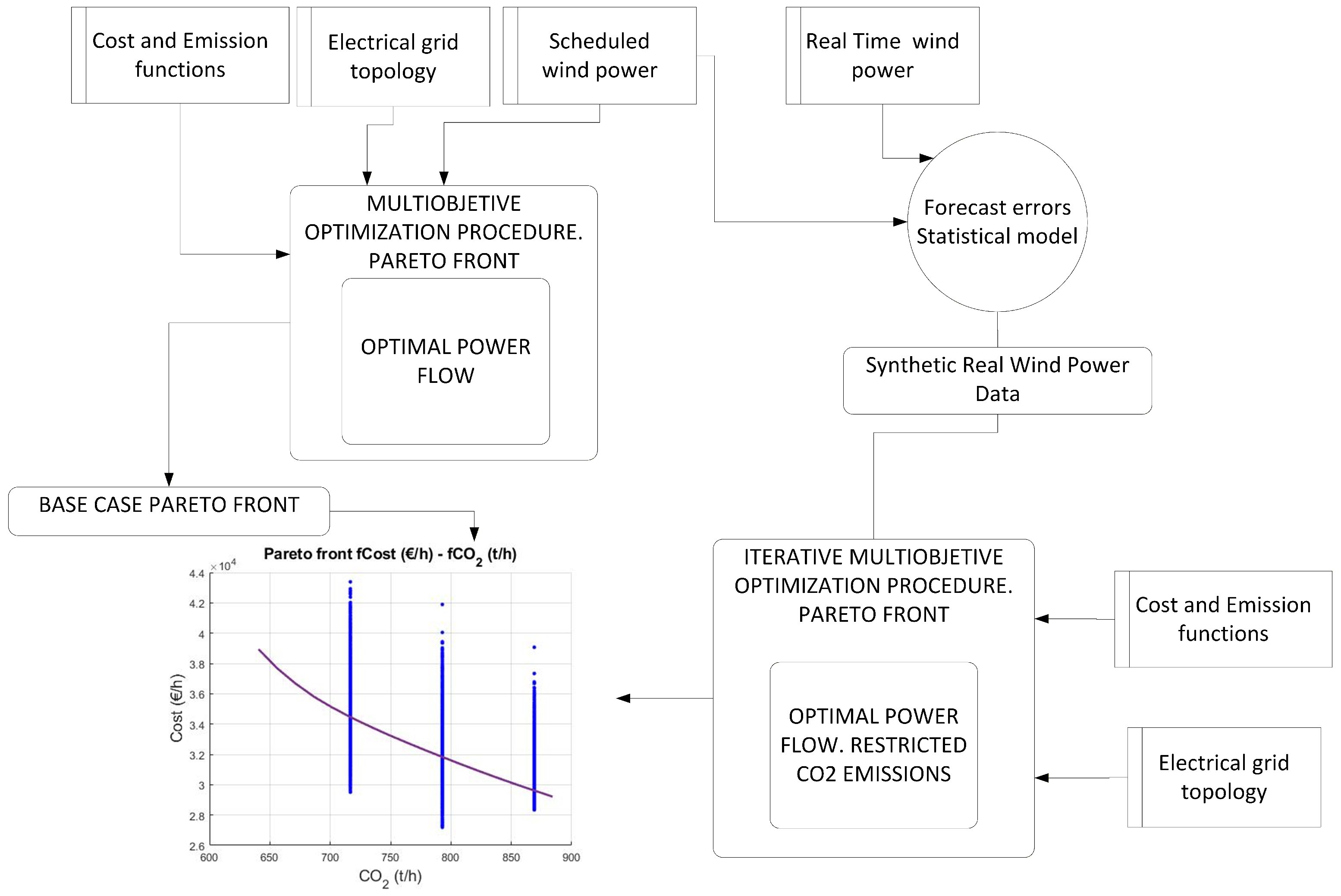Figure 1 illustrates the adopted methodology and serves as a frame of reference for the rest of the article.

A first multi-objective optimization is carried out, confronting the cost and CO₂ emissions functions, with the forecast reference wind production to determine the base Pareto front, which is the front or the set of optimal points that would be found if the wind production fit the forecast. Next, based on this result, a study is carried out on how the optimal generation costs change with the actual deviations of the wind energy production with respect to the forecast but complying with the restriction of not exceeding a certain amount of base-planned emissions. The obtained results show how conventional generation adapts to the variability of the wind resource, id est, the results show the optimal variations for the thermal generation when a renewable source deviates from the forecast production or from the offer.

3. Modelling of Cost and Emission Functions

To apply the multi-objective optimization model, it is necessary to characterize the thermal power plants used in the typical network. The cost and CO₂ emission functions were determined for lignite, domestic and imported bituminous coal, hard coal, and combined cycle plants.

The most direct way to model the behaviour of a thermal group is to adjust the measurements of the evolution of the magnitude to be studied as a function of load, and for this, it is necessary to have several reasonable measurements.

Several objectives could be modelled and studied as functions, such as hourly energy consumption, fuel mass, operating cost, CO₂ emissions, SO₂ emissions, NO_x emissions, and operating cost, by integrating CO₂ emissions into the emission permit price.

3.1. Cost Functions

The data needed to characterize the consumption curves of power plants is difficult to obtain. To carry out this study, a very comprehensive publication by the former Ministry of Industry and Energy (hereinafter MINER) [27] was consulted, which made available to the public the marginal consumption, average consumption, and start-up costs of each of the power plants existing in 1988. The heat-rate curves of thermal units were derived from real operational measurements at different load levels (full, 75%, and 50% load). The report classifies power plants by type. Although the data may seem outdated, the curves are valid for characterizing the behaviour of these power plants and serve to illustrate the methodology attempted to be shown in this article.

For the modelling of combined cycles, a 2 × 1 cycle with a GE 7FA.04 turbine rated at 480 MW at 15 °C was analysed based on data tables from the Bowie plant in Arizona [28].

The hourly energy consumption function ($f_e$) is expressed as a function of the heat-rate consumption ($f_{hr}$), measured in kJ/kWh, and the actual power of the power plant:

$$f_e\left(P\right)\left[{\displaystyle \frac{kJ}{h}}\right]=f_{hr}\left(P\right)\left[{\displaystyle \frac{kJ}{kWh}}\right]·P\left[kW\right]$$

(1)

The fuel consumption is obtained from the energy function and simply divided by the lower heating value (LHV) of the fuel:

$$f_{fuel}\left(P\right)\left[{\displaystyle \frac{kg}{h}}\right]={\displaystyle \frac{f_e\left(P\right)\left[\frac{kJ}{h}\right]}{LHV\left[\frac{kJ}{kg}\right]}}$$

(2)

To move to the operating-cost function ($f_c$), which is mainly represented by the cost of fuel, we must multiply by a factor of $k_c$, which is the cost of one kJ of the corresponding fuel:

$$f_c\left(P\right)\left[{\displaystyle \frac{ϵ}{h}}\right]=f_e\left(P\right)\left[{\displaystyle \frac{kJ}{h}}\right]·k_c\left[{\displaystyle \frac{ϵ}{kJ}}\right]$$

(3)

In general, almost all documents on dispatch or OPF [29,30,31,32] model the cost functions according to quadratic polynomial curves: $f_c=a·P^2+b·P+c$.

In [31], Lamont and Obessis used a model consistent with a cubic setup, without quadratic term, according to the following:

$$f_c=c+b·P+a·P^3$$

(4)

In [32], Gjengedal et al. modelled the cost function as follows:

$$f_c=b·P+a·P^2$$

(5)

In the MINER document [27], in addition to the test data (P, $f_{hr}$), the fitting parameters for each plant’s heat-rate consumption curves are provided, following nonlinear and linear models as follows:

$$f_{hr}={\displaystyle \frac{c}{P}}+b+a·P$$

(6)

$$f_{hr}=e+d·P$$

(7)

In this study, the first of the two models for the heat rate ($f_{hr}$) of all plants is followed, resulting in quadratic polynomial cost curves.

Table 1. Characteristics of the investigated fuels and power plants.

Power Plant	C (%)	S (%)	LHV (kJ/kg)	Fuel Cost (EUR/MWh)	${\mathit{P}}_{\mathit{N}}$ (MW)
Hard Coal	60	1.3	22,000	8	350
National Coal	60	1.3	22,400	8	225
Imported Coal	70	0.6	26,350	8	250
Brown Coal	33	4.5	14,650	4.673	350
Combined Cycle/Natural Gas	74.2	0	50,006.5	26	400

shows the fundamental characteristics of the fuels used by thermal power plants in the simulation. These factors include fuel composition, which is necessary for estimating CO₂ emissions, as well as the lower heating value (LHV), fuel cost, and rated power. The data on the characteristics of the fuels were taken from two theses on the environmental effects of the operation of the Spanish electricity system [33,34].

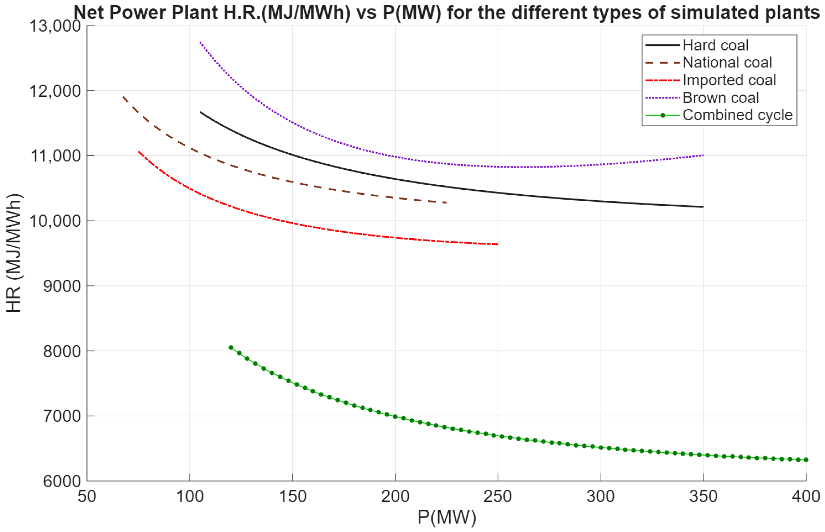
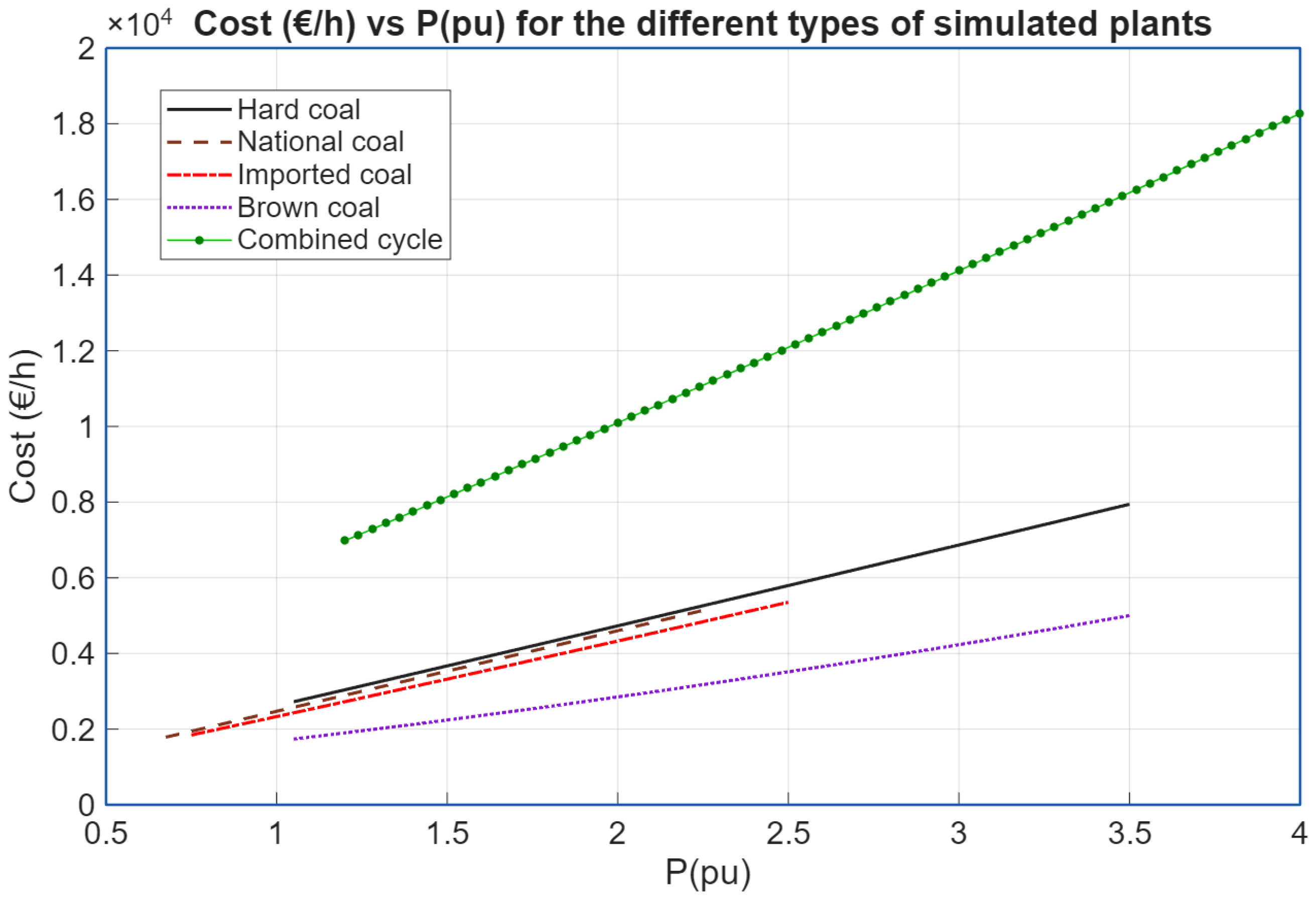
The heat-rate consumption functions of the generation groups classified by fuel type can be seen in Figure 2 and Figure 3, showing the associated cost functions.

3.2. CO₂ Emissions Functions

CO₂ emissions come from fuel, and it can be said that their evolution with power follows the trend of the fuel consumption curve multiplied by the emission factor per unit mass of fuel according to the combustion reaction, that is, if $w_c$ is the content per unit of C in the fuel, deduced from its elemental analysis, and recalling the following combustion reactions:

$$C+O_2\to C{O}_2$$

(8)

and taking into account the atomic masses of the elements and the molecular masses (CO₂: M.W. = 44 g), the following is obtained:

$$f_{C{O}_2}\left(P\right)\left[{\displaystyle \frac{kg}{h}}\right]=f_{fuel}\left(P\right)\left[{\displaystyle \frac{kg}{h}}\right]·w_c·{\displaystyle \frac{44}{12}}$$

(9)

If the carbon retention (unburned; $f_{c\_ash}$) is known per unit relative to the carbon content (C) data from the elemental analysis, the above function becomes

$$f_{C{O}_2}\left(P\right)\left[{\displaystyle \frac{kg}{h}}\right]=f_{fuel}\left(P\right)\left[{\displaystyle \frac{kg}{h}}\right]·w_c·{\displaystyle \frac{44}{12}}·\left(1-f_{c\_ash}\right).$$

(10)

The percentage of unburned carbon retention is usually a very low value, so complete combustion was assumed in the curves used in this article, but it is easy to introduce that factor if that information is available.

4. Multi-Objective Optimization

Multi-objective optimization involves multiple functions, which often conflict with each other. In this context, within the range of possible solutions, if one of the objective functions is to be improved by moving to a better solution, another of the objective functions will be penalized or compromised. This rate of compromise, which relates the improvement in one objective to the penalty in another, is known in technical literature as a “trade-off”.

There are numerous books, articles, and texts in which you can delve deeper and read about operations research, optimization, and methods or solvers for addressing optimization problems. A few sources on optimization and operations research in general include the classic work by Hillier and Liberman [35] and that of Chong and Zak [36]. There is also a wealth of scientific literature in specific books on multi-objective optimization, including those by Miettinen, Deb et al. [37] and Ehrgott [38]. To begin with, you can get a very clear idea of what multi-objective optimization is, the foundations and concepts that define it, and the methods and techniques used to carry it out by reading the summaries by Marler and Arora [39] and López Jaimes et al. [40]. Recently, there has been increased research interest in global optimization methods based on genetic and evolutionary algorithms, and there are also texts with very good introductions to the theory of multi-objective problems; worth mentioning is that by Coello et al. [41] and the thesis by Zitzler [42].

The process of systematic and simultaneous optimization of a set of objective functions is called multi-objective optimization (hereafter, MOO), and the problems to which these techniques are applied are called multi-objective optimization problems (hereafter, MOPs).

4.1. Definition of a Multi-Objective Optimization Problem

It is assumed, without loss of generality, that problems are posed in terms of minimization. A maximization problem is equivalent to a minimization problem, since

$$Maxf\left(x\right)=Min(-f(x\left)\right).$$

(11)

A multi-objective problem can be formulated generically as follows:

$$\begin{array}{c}\hfill minimizef\left(x\right)={\left[f_1\left(x\right),f_2\left(x\right),\cdots \cdots ,f_m\left(x\right)\right]}^T\\ \hfill subjectto{g}_j\left(x\right)\le 0,j=1,2,\cdots \cdots ,p\\ \hfill h_l\left(x\right)=0,l=1,2,\cdots \cdots ,q\\ \hfill forx={\left[x_1,x_2,\cdots \cdots ,x_n\right]}^T\end{array}$$

(12)

where $x\in {\Re }^n$ is a vector of n independent decisions or design variables, the values of which are to be found in the optimization problem; $f\in {\Re }^m$ is a vector of m objective functions, with each of the functions’ ($f_i\left(x\right)$) components called objectives, criteria, or goals; $g_j$ is one of the p inequality constraints to which the problem is subject; and $h_l$ is on one of the q equality constraints to which the problem is subject.

The objective function vector (f:${\Re }^n\to {\Re }^m$)is composed of m objective scalar functions ($f_i:{\Re }^n\to \Re (i=1,2,\dots ,m;m\ge 2)$), and it defines the relationship between the decision or design space (${\Re }^n$) and the space of functions and objectives (${\Re }^m$).

The feasible design space (feasible design space or restricted decision set) is defined as the set (X) of values in the design space or variable that satisfies the constraints. The image set of that set defines the target feasible space (Y). Unlike optimization with a single objective function and a single solution, in multi-criteria optimization, the solution is a set of points that satisfy the concept of optimality. In MOPs, the most widely accepted concept for determining whether a point is optimal or not is Pareto optimality or Pareto dominance. This criterion was initially proposed by Francis Ysidro Edgeworth in 1881 [43] but was formalized and generalized by Vilfredo Pareto in 1896 [44].

In this text, terminology that indicates that one point improves or surpasses another is used to indicate that former is more optimal than the latter, whereas worsening means that it is less optimal.

A solution ($x_1\in \mathit{X}$) is said to dominate (in the Pareto sense) another vector ($x_2\in \mathit{X}$) if it is true that point $x_1$ is no worse than $x_2$ in any of the objective functions and, in at least one of them, it improves upon it.

A vector ($x^{*}$) is said to be strictly Pareto-optimal if and only if

$$\begin{array}{c}\hfill x^{*}\in XisstrictParetooptimal\iff \neg \exists x\in X \mid \\ \hfill f_i\left(x\right)\le f_i\left(x^{*}\right)\forall i\in \{1,2,\cdots \cdots ,m\}\\ \hfill and\\ \hfill \exists i\in \{1,2,\cdots \cdots ,m\}:f_i\left(x\right)<f_i\left(x^{*}\right),\end{array}$$

(13)

that is, a point is strictly Pareto-optimal if there are no other points that improve on it in any function without worsening it in at least one other function.

The images of strict Pareto optima are located at the boundary of the feasible objective space. Some MOO algorithms can also produce points very close to this condition without actually reaching it, and these are also be of interest. Of particular interest are weak Pareto optima, which are those that cannot be improved upon by any other point in all functions at the same time but which can be equalled in some.

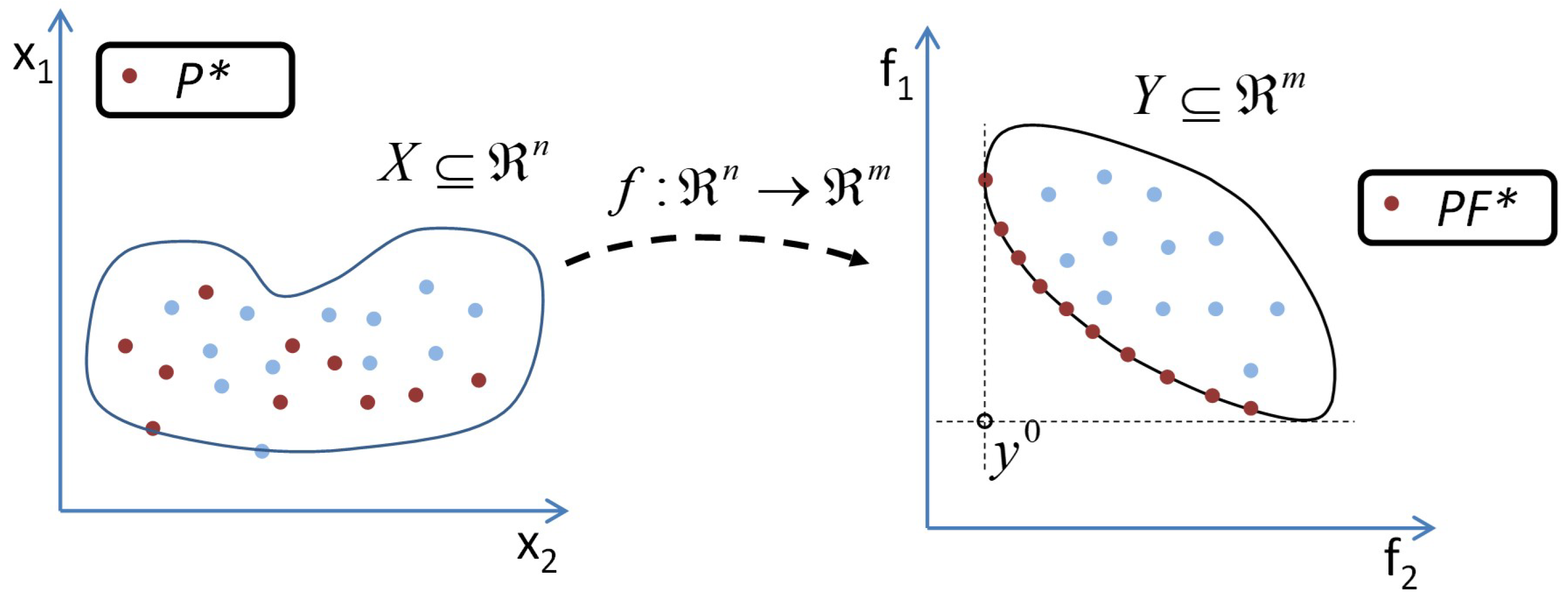
The subset of strictly Pareto-optimal points within the feasible decision space defines the Pareto-optimal set (P*), and the subset of objective values of that set is called the Pareto front (PF*).

The Pareto front lies on the optimal boundary or contour of the feasible objective space, but the set of Pareto optimal solutions does not necessarily do so in its space (see Figure 4).

There are different methods for finding the set of solutions that define the Pareto front. In the studied case, the $\epsilon$-constraint method was used.

4.2. $\epsilon$-Constraint Method

This method basically consists of selecting one objective—the most interesting or significant one—as the objective function to be minimized and treating the rest of the criteria as constraints, sweeping them between their extreme values. It was introduced by Haimes et al. in 1971 and was analysed by detail in Chankong and Haimes in 1983 [45].

From a methodological standpoint, the $\epsilon$-constraint technique is particularly well suited for power-system dispatch problems in which regulatory or policy-driven limits must be explicitly enforced. Unlike weighted-sum approaches, which may fail to recover non-convex regions of the Pareto front and require subjective tuning of weighting coefficients, the $\epsilon$-constraint method allows the system operator to directly impose admissible bounds on secondary objectives, such as emissions or environmental impact indicators. Yamaguti et al. [12] demonstrated that convex multi-objective formulations combined with $\epsilon$-type constraints yield well-structured and interpretable Pareto fronts, facilitating decision making in environmentally constrained OPF problems. Similarly, Villacrés and Carrión [13] showed that hybrid $\epsilon$ constraint-based approaches enhance solution transparency and robustness, especially when integrated with satisfaction or fuzzy decision layers. Recent overview studies, such as that by Nyingu et al. [11], further confirm that $\epsilon$-constraint formulations remain among the most reliable and scalable techniques for multi-objective load flow and dispatch problems in modern power systems.

The multi-objective problem posed under the $\epsilon$-constraint method can be formulated as follows:

$$\begin{array}{c}\hfill minimize{f}_k\left(x\right)\\ \hfill subjectto{f}_i\left(x\right)\le {\epsilon }_i\forall i=1,2,\cdots \cdots ,m,i\ne k\\ \hfill x\in X\end{array}$$

(14)

With this method, all solutions on the Pareto front can be found, whether convex or not.

However, in order to perform a complete and consistent exploration of the contour of interest using the $\epsilon$-constraint method, the problem must be accessible to certain information: the extremes of the objectives to be taken as constraints must be calculated in advance in order to scan the problem by varying the parameters of the constraints between these limit values. In other words, it must be possible to previously calculate the values of $f_{min}^i$ and $f_{max}^i\forall i\ne k$, iteratively obtaining the minimum of the objective function ($f_k$) as the value of ${\epsilon }_i$ is changed progressively from one extreme to the other, increasing it with a suitable step to obtain the desired meshing and distribution.

When the problem is convex and the main objective function is strictly convex, the solutions are strictly Pareto-optimal. However, when strict optimality conditions cannot be guaranteed or proven and if it is necessary to ensure that the obtained solutions are on the Pareto front, there are mathematical tests to discriminate whether the solutions are on the Pareto front or not [36,46].

5. Analysis and Modelling of Wind Energy Production Data

Accurate modelling of wind power and its uncertainty has advanced significantly in recent years. Romo Perea et al. [47] validated “three new measure–correlate–predict models for the long-term prospection of the wind resource”, demonstrating improved techniques for long-term wind resource assessment based on short-term measurements. For operational time scales, Jeon and Taylor [48] used “conditional kernel density estimation for wind power density forecasting” and showed that conditional kernel methods can effectively model the non-Gaussian distributions of wind power under different meteorological conditions. This supports the use of kernel-based distributions in the present paper to model wind forecast errors.

Several studies have combined deep learning with non-parametric density estimation for short-term wind power forecasting and uncertainty analysis. Zhou et al. [49] proposed “wind power prediction based on LSTM networks and nonparametric kernel density estimation”, where long short-term memory (LSTM) networks are used for point forecasts and kernel density estimation is used for probabilistic forecasts. They reported that this hybrid approach captures heavy tails and asymmetries in forecast error distributions more accurately than simple parametric models. Gu et al. [26] presented “short-term forecasting and uncertainty analysis of wind power based on long short-term memory, cloud model and non-parametric kernel density estimation”, again highlighting that non-parametric KDE effectively represents complex uncertainty structures in wind power.

Beyond power itself, Dong et al. [50] introduced “a novel paradigm for multi-step wind speed prediction: a hybrid system based on decomposition and weighted ensemble approach enhanced by Gaussian kernel function”, using Gaussian kernels within an ensemble to better capture the stochastic dynamics of wind speed. These works collectively show that kernel-based statistical models are now a standard tool for representing non-Gaussian wind uncertainty, which justifies the kernel-density approach used in this paper for the generation of synthetic deviations.

Probabilistic scenario generation methods are also central to the integration of wind uncertainty into operational planning. Yoshida et al. [51] described “a stochastic scheduled operation of wind farm based on scenarios of the generated power with copula”, where copula-based dependence modelling is used to generate realistic joint scenarios for wind power across time. Xu et al. [52] presented a “data-driven risk-averse two-stage optimal stochastic scheduling of energy and reserve with correlated wind power” in which correlated wind scenarios are generated from historical data and used in a two-stage stochastic program. Zhang et al. [53] proposed a “stochastic optimization operation of the integrated energy system based on a novel scenario generation method”, again using data-driven scenario techniques to propagate renewable uncertainties through an integrated energy system. The methodology adopted in this paper—fitting kernel distributions to empirical forecast errors and sampling many synthetic deviation scenarios—follows this data-driven, scenario-based tradition.

There are usually mechanisms and markets for buying and selling energy in which the process of selling energy takes place 24 h before consumption. This is the case with the MIBEL electricity market, the joint market for Spain and Portugal. This type of market requires the most accurate estimate possible of wind energy production in order to minimize deviations caused by forecasting errors. In this context, Wang et al. [10] suggested that the integration of renewable energies into such markets requires robust formulations to effectively manage technical and economic uncertainties. Although these deviations can be offset by deviations in demand, this study does not take into account the relationship between deviations in generation and demand.

Statistical Model

Deviations from scheduled production involve many factors, such as predicted and actual wind speeds, wind farm performance, and market bidding strategies. This means that the distribution of the aforementioned prediction errors does not necessarily follow standard statistical distributions, such as the normal distribution. Recent literature, including the work of Zhang et al. [53], highlights that, since these errors are often non-Gaussian, advanced probabilistic modelling is required to ensure grid reliability.

This study aims to examine the influence of wind energy deviations on both the costs associated with certain emission levels and the details of which conventional power plants must bear the burden of such errors.

To determine the influence of wind energy deviations on the results of multi-objective optimization, the employed calculation methodology involved generating a random series of deviations from a preliminary wind power generation offer. Each resulting deviation generates a scenario that defines a Pareto front. This front has an associated probability of occurrence, linked to the inherent probability of the deviation, but is subsequently adjusted to the constraints of the electrical system and CO₂ emissions.

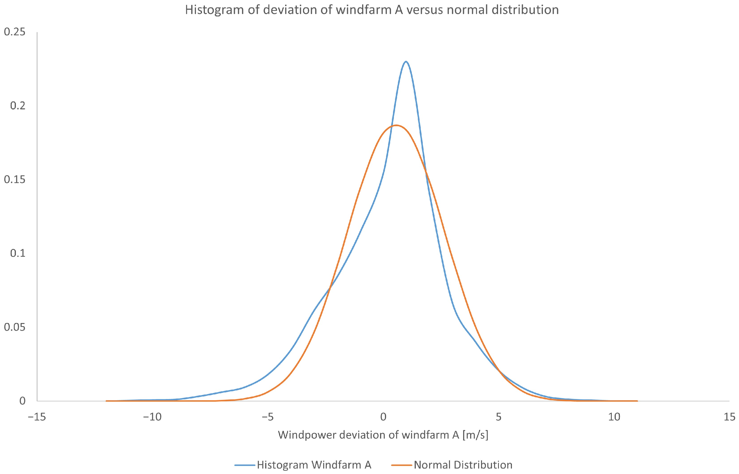
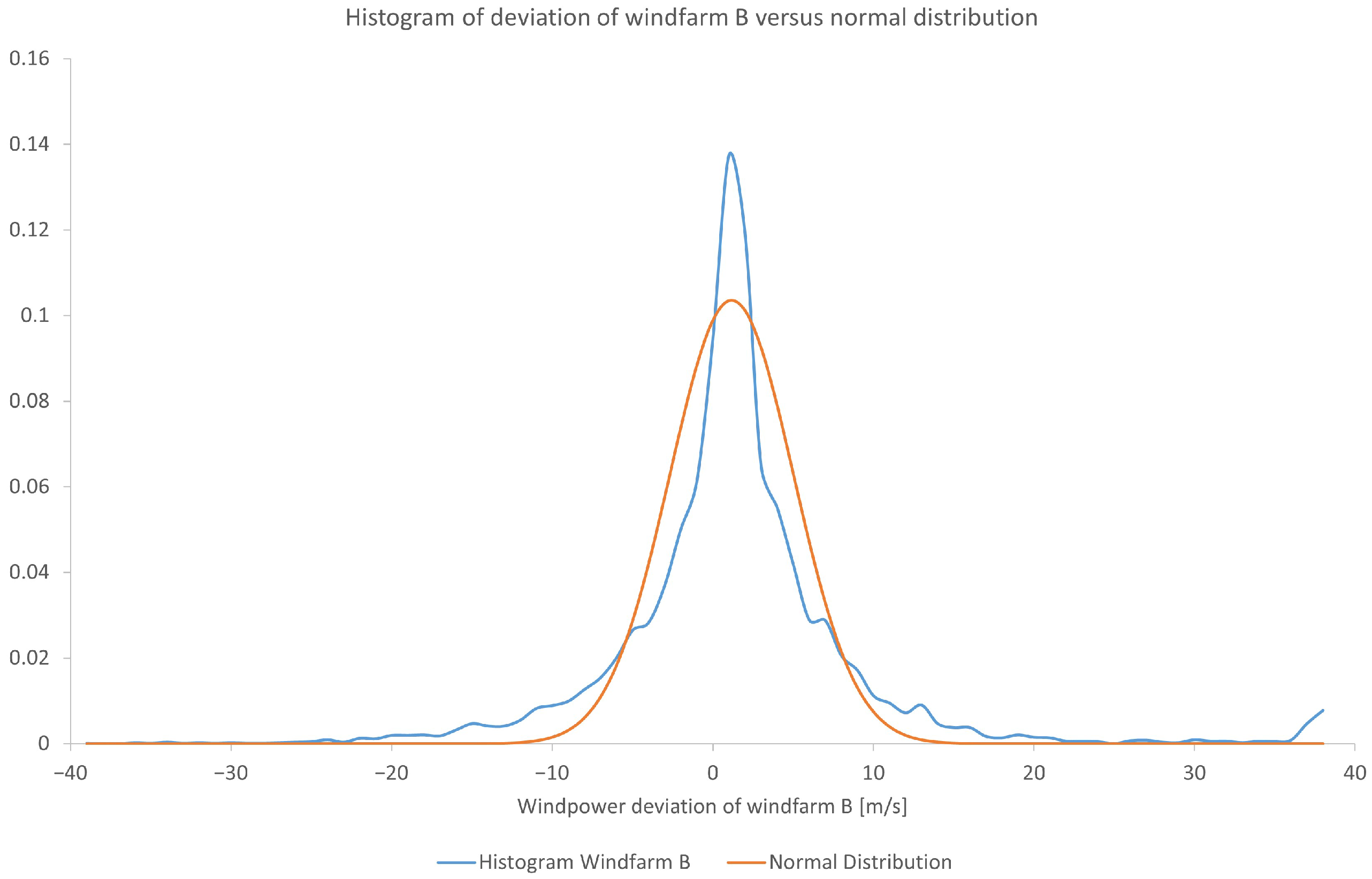
In this study, the analysis was based on actual and planned wind power production data from two operational wind farms: Farm A and Farm B. Farm A has an installed capacity of 13 MW, while Farm B operates at a nominal capacity of 46.6 MW. The dataset includes 9503 hourly records of planned and actual production for Farm A and 8760 records for Farm B. The deviations are considered as ${\epsilon }_{Ah}={\widehat{P}}_{wA,h}-P_{wA,h}$, that is, the difference between programmed and actual wind energy production. The normal distribution that best fits the deviation of histograms is also represented in Figure 5 and Figure 6 to verify its fit. It is observed that the data does not fit very well with this distribution, so alternatives are sought, with the Kernel distribution proving to be the best fit.

As a result of modelling the deviation histograms, the forecasts in Farm A are slightly lower, on average, than the actual generation, and the opposite is true for Farm B.

Table 2. Summary of general prediction error data.

Program Deviation	Nominal Power	Mean Value of Prediction Errors	Statistical Deviation of the Prediction Errors
FarmA	13 MW	−0.277 MW	2.77 MW (19%)
FarmB	46.6 MW	0.92 MW	7.67 MW (16.5%)

shows the mean values and standard deviations for both reference farms.

For the statistical modelling of the deviations and following other researchers, it was decided to use the Kernel statistical distribution, which allows for a better fit to the calculated histograms.

This type of distribution smooths the data histogram. To do this, each sample is associated with a smoothing function, and the probability density function is generated as a weighted sum of the smoothing functions. If n samples are available, the probability density estimate can be expressed as follows:

$$\widehat{pdf}\left(x\right)={\displaystyle \frac{1}{n·h}}·\sum _{i=1}^{n}K·{\displaystyle \frac{x-x_i}{h}}$$

(15)

where h is the bandwidth and $K·{\displaystyle \frac{x-x_i}{h}}$ is the smoothing function, which can range from a square function to a normal, triangular, or Epanechnikov function. The estimation of this distribution was carried out using the Matlab (MATLAB2024b) “fitdist” function.

The electrical system under study is a 57-node network with a demand of 1250.8 MW. Reference Farms A and B are too few and too small to have an influence on the network’s behaviour. Therefore, it was decided to scale the data from both wind farms so that they reached an order of 20% of the total demand to be covered, as well as to generate synthetic data from them that could be used to represent wind farms at different nodes of the network.

Given that there is not a large amount of available data of foreseen and actually produced wind power, a statistical distribution model fitting this behaviour was used in order to facilitate the generation of a matrix of synthetic deviation data as broad as desired. In our case, 2000 wind deviated data were generated for each wind farm, making it possible to study how the solutions of multi-objective optimization, in terms of cost and emissions, vary with respect to the base case when wind errors are introduced.

To obtain synthetic wind generation data for wind farms with different installed capacities, the following procedure was adopted:

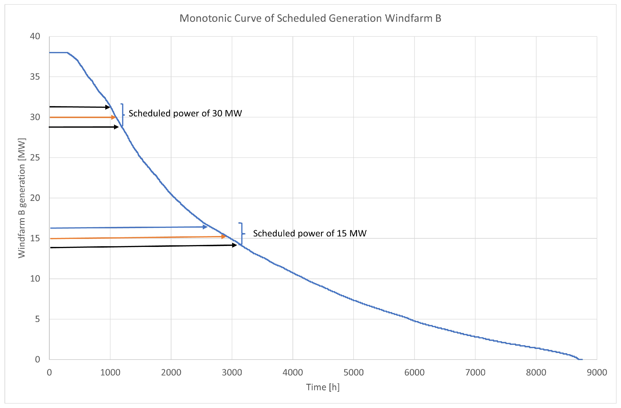
1.

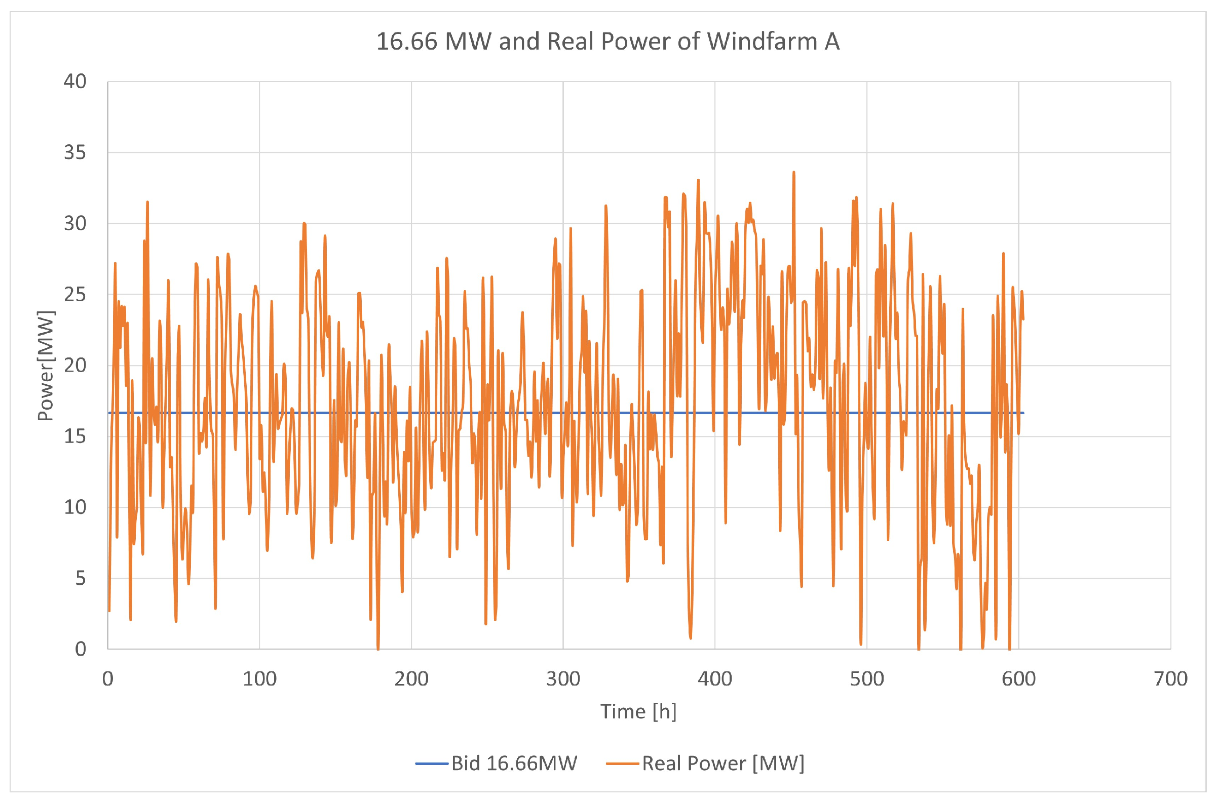
Ordering of the estimated and actual production data in descending order of estimated power (see Figure 7 with an example of Farm B, where two schedule powers were selected, as reference);

2.

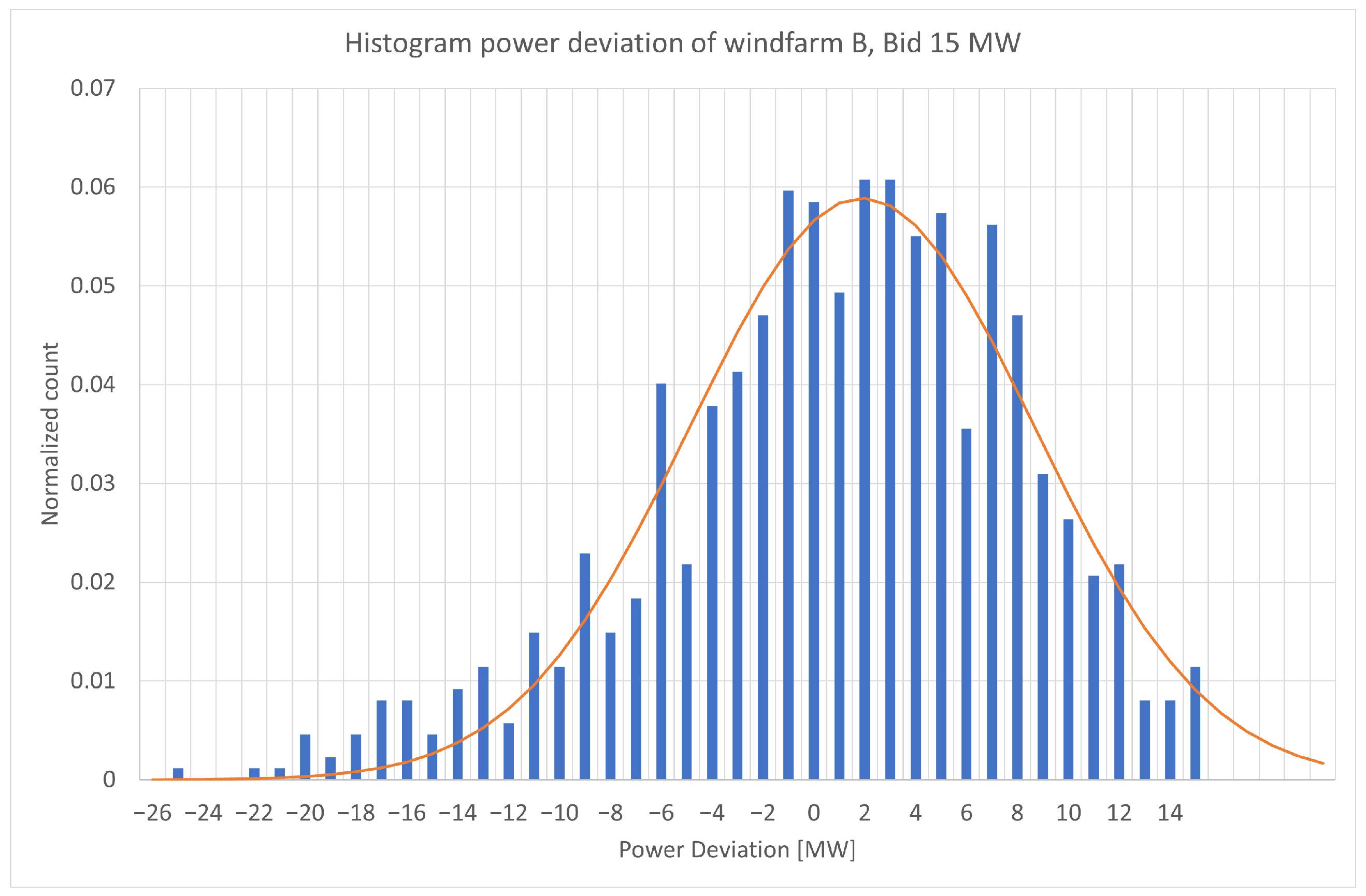
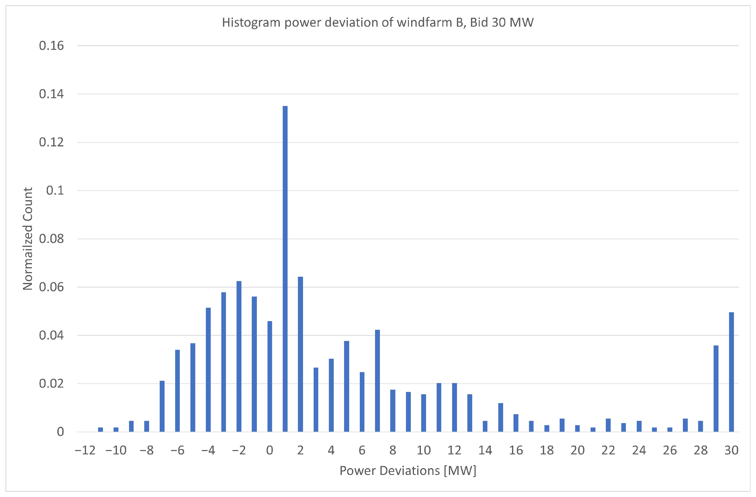
Selection of the estimated power intervals with a width of 1 MW for Farm A and 5 MW for Farm B, along with the actual production associated with the estimated values. The characterisation of the deviations for each offer is calculated by studying the deviations that occurred over time for offers close to the offer made. For example, Figure 7 shows the deviations associated with the offer of $P_{Bid,i}^{WindB}=30\mathrm{MW}$, and $P_{Bid,i}^{WindB}=15\mathrm{MW}$ comprises an interval around the offer. These values are scaled to the capacities of the six generated synthetic wind farms. The central value of the estimated power interval represents the wind farm’s market bid.

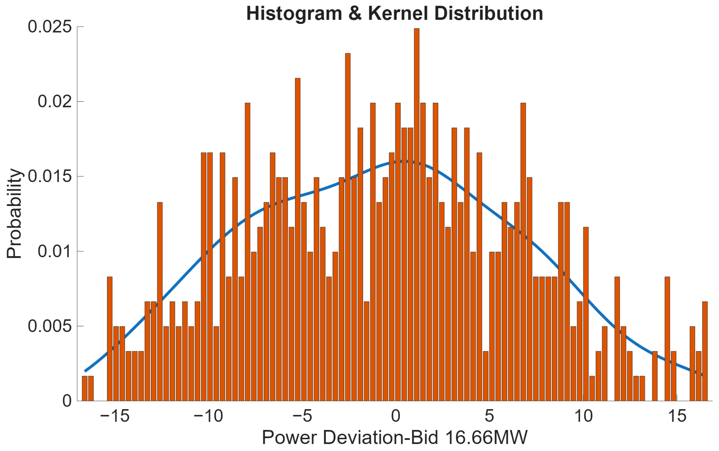
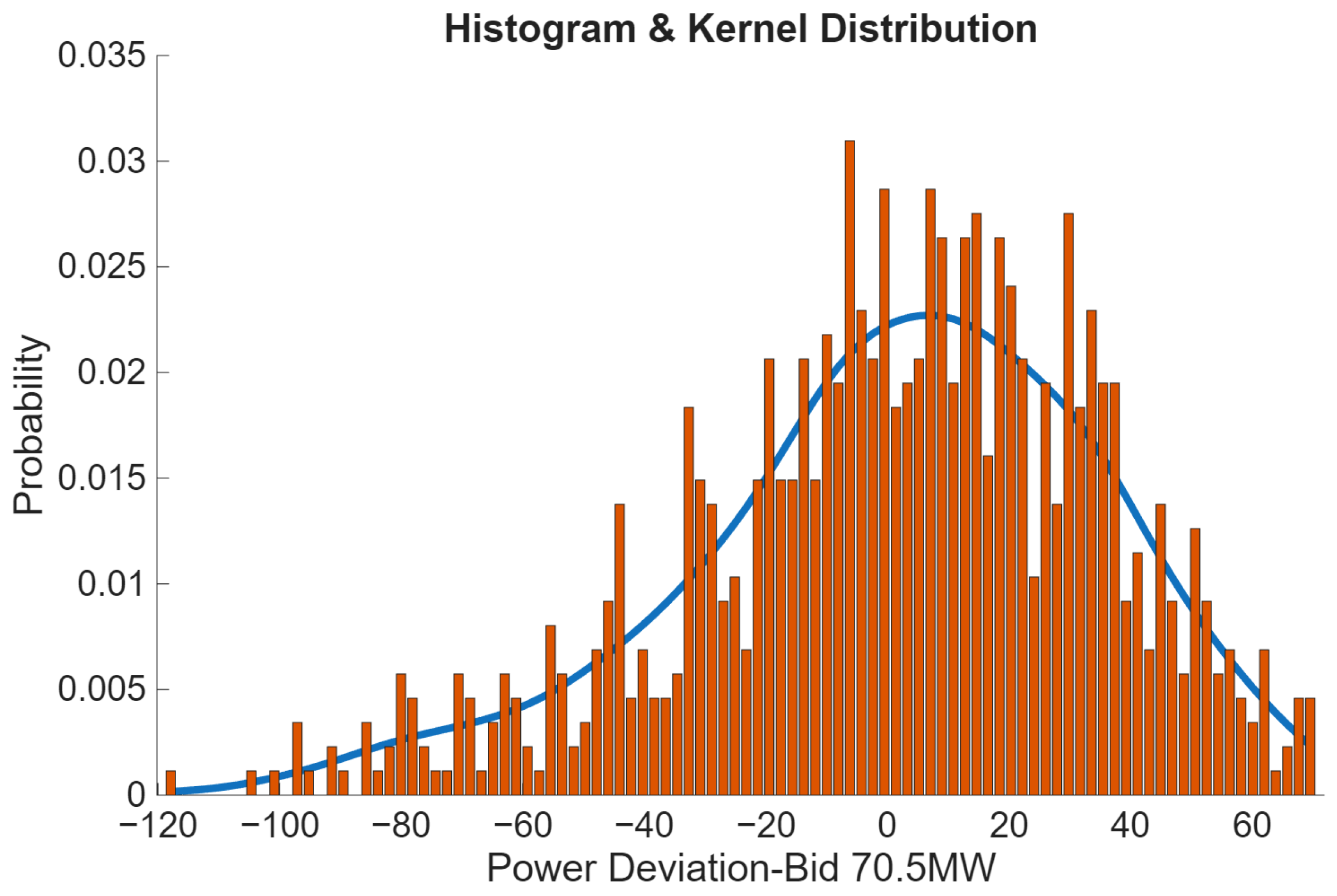
It can be observed how these deviations change from one offer to another (Figure 8 and Figure 9) and do not follow a normal distribution.

3.

To generate an array of actual production values associated with the market bid, the kernel function that best represents the resulting deviations for each interval was estimated based on the actual deviations corrected for the synthetic wind farm’s bid. The prediction error associated with the forecasted offer (${\epsilon }_{Bid,i}^{WindB}$) is calculated from the set of deviations associated with the bid bin, scaled to the value of the forecasted offer ($P_{Bid,i}^{WindB}$):

$$\begin{array}{c}\hfill {\epsilon }_{Bid,i}^{WindB}={\displaystyle \frac{{\widehat{P}}_{wB,h}-P_{wB,h}}{{\widehat{P}}_{wB,h}}}·P_{Bid,i}^{WindB}\\ \hfill where{\widehat{P}}_{wB,h}\in \left[P_{Bid,i}^{WindB}-\Delta ·P_{Bid,i}^{WindB}·P_{Bid,i}^{WindB}+\Delta ·P_{Bid,i}^{WindB}\right]\end{array}$$

(16)

where ${\widehat{P}}_{wB,h}$ is the estimated wind power generation in hour h, $P_{wB,h}$ is the actual wind power generation in hour h, and $\Delta ·P_{Bid,i}^{WindB}$ represents the increment of estimated wind power generation and the size of the bin interval.

Both the offered powers and the originated deviations were scaled so that the wind farms had a significant weight, stretching Farm A from its actual 13 MW to a 30.94 MW farm and to a 61.1 MW famr, as well as Farm B from its 46.6 MW to a nominal power of 218.5 MW and a nominal power of 110.67 MW.

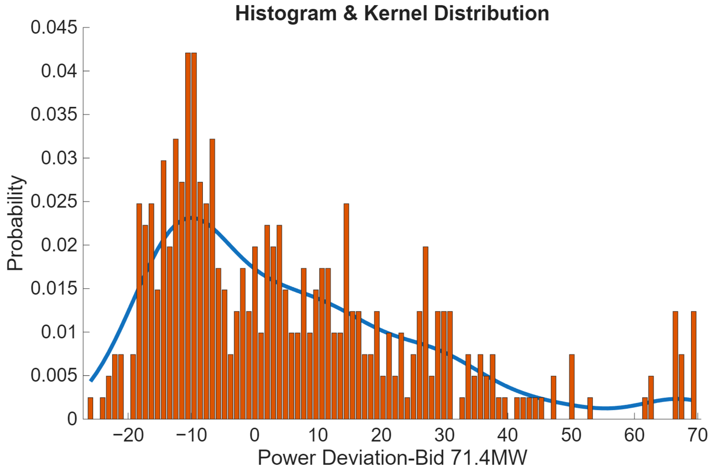
The estimation of the kernel distributions, which are the best fits of the histograms of the offer deviations, was carried out in Matlab. Later, arrays of random deviations were generated following the kernel distributions associated with each offer (Figure 10).

The results of the adjustment of the kernel distributions of the offers are presented in

Table 3. Estimation of kernel distribution models.

Max Power	Bid	Kernel	Bandwidth
30.94 MW	16.66 MW	Normal	2.40774
30.94 MW	28.56 MW	Normal	1.02929
61.1 MW	32.9 MW	Normal	4.75477
61.1 MW	56.4 MW	Normal	2.03264
218.55 MW	70.5 MW	Normal	8.80877
110.67 MW	71.4 MW	Normal	6.00953

.

Figure 11, Figure 12 and Figure 13 show the adjustment of the deviations for the studied offers of 16.66 MW, 70.5 MW, and 71.4 MW.

4.

Finally, random arrays of actual production were generated for the different market bids in order to simulate the different scenarios.

6. Approach to the Multi-Objective Optimization Model

Before describing how the multi-objective optimization problem is formulated, it is necessary to detail the formulation of the optimal load flow problem, in which we want to minimize a single objective function ($f^k$), subject to the constraints of power balance at the buses, power transportation capacity limits for the transmission lines, admissible voltage, and generated powers values.

First, the formulation of a single objective problem ($f\left(x\right)$) is recalled generically as follows:

$$\begin{array}{c}\hfill minimizef\left(x\right)\\ \hfill subjectto{g}_j\left(x\right)\le 0,j=1,2,\cdots \cdots ,p\\ \hfill h_l\left(x\right)=0,l=1,2,\cdots \cdots ,q\\ \hfill forx={\left[x_1,x_2,\cdots \cdots ,x_n\right]}^T\end{array}$$

(17)

Particularizing it to our purpose and writing it in the nomenclature of the variables of an electrical power system yields the following:

$$\begin{array}{c}\hfill minimize{f}^k=\sum _{i=1}^{ng}\left(a_i^k·P_{gi}^2+b_i^k·P_{gi}+c_i^k\right),k\in \{1,2,\cdots ,n_f\}\\ \hfill forx={\left[P_{g1},\cdots ,P_{gng},Q_{g1},\cdots ,Q_{gng},V_1,\cdots ,V_{nb},{\delta }_1,\cdots ,{\delta }_{nb}\right]}^T\\ \hfill subjectto\\ \hfill Inequalityconstraints,g_j\left(x\right)\le 0:\\ \hfill S{l}_{jk}\left(x\right)-S_{max,i}\le 0;j=ic(i,1),k=ic(i,2),\forall i\in \{1,2,\cdots ,n_c\}\\ \hfill S{l}_{kj}\left(x\right)-S_{max,i}\le 0;j=ic(i,1),k=ic(i,2),\forall i\in \{1,2,\cdots ,n_c\}\end{array}$$

(18)

$$\begin{array}{c}\hfill Equalityconstraints,h_l\left(x\right)=0:\\ \hfill f_{pi}\left(x\right)-P_i=0;\forall i\in \{1,2,\cdots ,n_b\}\\ \hfill f_{qi}\left(x\right)-Q_i=0;\forall i\in \{1,2,\cdots ,n_b\}\\ \hfill VariableLimits:\\ \hfill V_{min}\le V_i\le V_{max};\forall i\in \{1,2,\cdots ,n_b\}\\ \hfill P_{gmin,i}\le P_{gi}\le P_{gmax,i};\forall i\in \{1,2,\cdots ,n_g\}\\ \hfill Q_{gmin,i}\le Q_{gi}\le Q_{gmax,i};\forall i\in \{1,2,\cdots ,n_g\}\\ \hfill {\delta }_i\in \left(-\pi ,+\pi \right);\forall i\in \{1,2,\cdots ,n_b\};{\delta }_1=0\end{array}$$

where

• $S{l}_{jk}\left(x\right)=\left|{\overline{V}}_j·{\left[{\overline{V}}_j·{\displaystyle \frac{{\overline{y}}_{sjk}+{\overline{y}}_{pjk}}{\overline{a}*·\overline{a}}}-{\overline{V}}_k·{\displaystyle \frac{-{\overline{y}}_{sjk}}{\overline{a}*}}\right]}^{*}\right|$
• $S{l}_{kj}\left(x\right)=\left|{\overline{V}}_k·{\left[{\overline{V}}_k·\left({\overline{y}}_{sjk}+{\overline{y}}_{pjk}\right)-{\overline{V}}_j·{\displaystyle \frac{-{\overline{y}}_{sjk}}{\overline{a}}}\right]}^{*}\right|$
• $f_{pi}\left(x\right)={\sum }_{k=1}^{n_b}{V}_i·V_k·Y_{ik}·cos({\delta }_k-{\delta }_i+{\gamma }_{ik}),or{f}_{pi}\left(x\right)=\Re ({\sum }_{k=1}^{nb}{\overline{V}}_i^{*}·{\overline{V}}_k·{\overline{Y}}_{ik})$
• $f_{qi}\left(x\right)=-{\sum }_{k=1}^{n_b}{V}_i·V_k·Y_{ik}·sin({\delta }_k-{\delta }_i+{\gamma }_{ik}),or{f}_{qi}\left(x\right)=-\Im ({\sum }_{k=1}^{n_b}{\overline{V}}_i^{*}·{\overline{V}}_k·{\overline{Y}}_{ik})$
• $P_i=P_{gi}-P_{di}$
• $Q_i=Q_{gi}-Q_{di}$

and where $n_b,n_g$, and $n_c$ are the number of nodes (or buses) in the system, the number of generation nodes, and the number of branches or connections between buses; $ic$ is an array ($n_c\times 2$) that contains the starting and ending positions of the branches of the network; $n_f$ is the number of functions for which the system has been characterised (in a single target OPF, only one of them is minimised; $S{l}_{jk}$ and $S_{max,i}$ are the modulus of the power flow in the branch between nodes j and k and the transport capacity of that branch; ${\overline{V}}_i,V_i,{\delta }_i;i\in \{1,2,\cdots ,nb\}$ represents the complex voltages, their modulus, and their angle at each bus; $P_{gi},Q_{gi};i\in \{1,2,\cdots ,nb\}$ represents the active and reactive powers generated at the buses; $P_{di},Q_{di};i\in \{1,2,\cdots ,nb\}$ represents the active and reactive powers demanded at the buses; ${\overline{Y}}_{ik},{\overline{Y}}_{ii};i,k\in \{1,2,\cdots ,nb\}$ represents the off-diagonal and diagonal terms of the network admittance matrix; ${\overline{Y}}_{sjk},{\overline{Y}}_{pjk};j,k\in \{1,2,\cdots ,nb\}$ represents the series and parallel admittances of the pi diagram of the connection lines between buses j and k of the electrical system; and $\overline{a}$ introduces the possibility of considering the existence of regulating transformers in the lines (the normal case of a simple line has no regulating transformer, and in that case, $\overline{a}$ is the real unit).

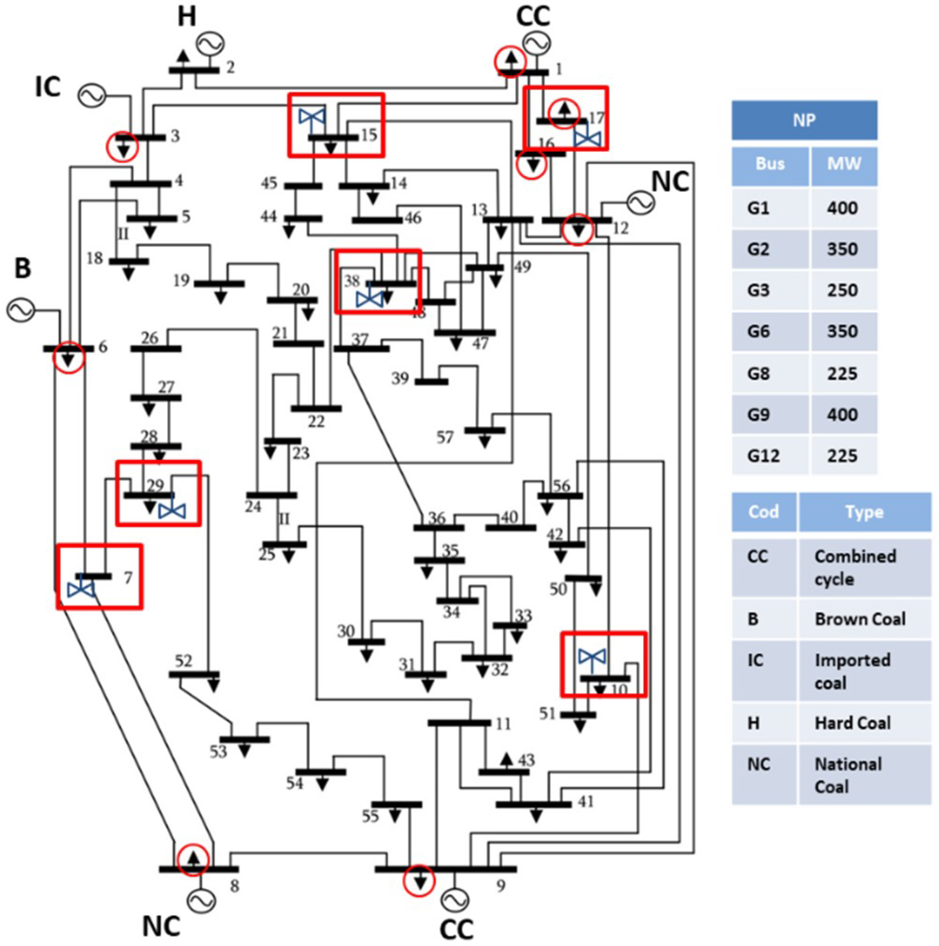
The system considered in this study is the network of the IEEE-57 case—a network with 57 buses, 80 lines, and a demand of 1250.8 MW. Figure 14 indicates the location of the thermal power plants. The locations of the main loads are depicted with circles, and wind power plants are indicaed with rectangles.

In the simulation reported in this paper, wind generation situations were introduced in six nodes of the network—the igw nodes (17, 38, 7, 10, 29, and 15), simulating the scene of the offered generation ($P_{gw}$ [MW] = [16.66, 28.56, 32.9, 56.4, 70.5, 71.4]) as the basis, with 276.42 MW of total wind power. The remainder of this study deals with the deviation of different registered situations from actual power from that offer.

To introduce the generation of wind power in these nodes, an additional condition is added to the previous algorithm:

$$P_{di}=P_{di}-P_{gwi},i=igw\left(j\right),\forall j\in \{1,\cdots ,n_w\}$$

(19)

where $n_w$ is the number of nodes with wind generation in the system (in this article, $n_w$ = 6) and $igw$ is a vector (1$\times$$n_w$) that contains the positions of the nodes with wind generation.

In this way, the generation of wind energy is simulated as a negative demand in the corresponding nodes, and it is always accepted by the network, regardless of the situation of the electrical variables or the rest of the generation of the system.

Once considering the formulation of an OPF, it is possible to proceed to the proposal of a multi-objective optimization for two functions ($n_f$ = 2) in the case of this article: the cost and the CO₂ emissions functions. To apply the $\epsilon$-constraint method, as explained above, the first thing to do is to calculate the maximum and minimum of the studied functions. The pseudo code used to do this with the k handled functions is shown below:

$$\begin{array}{c}\hfill fork=1:n_f\\ \hfill Minimize\\ \hfill f^k\left(x\right)=\sum _{i=1}^{n_g}\left(a_i^k·x_i^2+b_i^k·x_i+c_i^k\right),k\in \{1,2,\cdots ,n_f\}\\ \hfill subjectto\\ \hfill g_{opf}\left(x\right)\le 0\\ \hfill h_{opf}\left(x\right)=0\\ \hfill x={\left[x_1,x_2,\cdots ,x_{2·n_g+2·n_b-1}\right]}^T\\ \hfill f_{extr(k,1)}=f_{min}^k\\ \hfill Minimize\\ \hfill v^k\left(x\right)=-f^k\left(x\right)=-\sum _{i=1}^{n_g}\left(a_i^k·x_i^2+b_i^k·x_i+c_i^k\right),k\in \{1,2,\cdots ,n_f\}\\ \hfill subjectto\\ \hfill g_{opf}\left(x\right)\le 0\\ \hfill h_{opf}\left(x\right)=0\\ \hfill x={\left[x_1,x_2,\cdots ,x_{2·n_g+2·n_b-1}\right]}^T\\ \hfill f_{max}^k=-v_{min}^k\\ \hfill f_{extr}(k,2)=f_{max}^k\\ \hfill end\end{array}$$

(20)

Thus, the minimum values ($f_{min}^k$) and maximum values ($f_{max}^k$) of the $n_f$ functions are stored in matrix $f_{extr}$ with dimensions of $n_f$$\times$2.

With the previous values, the objective functions are normalized because, otherwise, the difference in magnitudes—and not their importance—can condition the optimization. Thus, the new normalized objectives are expressed as follows:

$$f_n^k={\displaystyle \frac{f^k\left(x\right)-f_{min}^k}{f_{max}^k-f_{min}^k}}\forall k\in \{1,2,\dots \dots ,n_f\}$$

(21)

With this normalization, the objective functions are bounded between 0 and 1.

Once the functions have been normalized, the multi-objective optimization of the two chosen functions can be carried out. The pseudo code of the algorithm to do this, sweeping n + 1) points, is written as follows:

$$\begin{array}{c}\hfill p={\displaystyle \frac{1}{n}};{\epsilon }_i=1;\\ \hfill while{\epsilon }_i\ge 0\\ \hfill Minimize{f}_n^k\left(x\right);x={\left[x_1,x_2,\cdots ,x_{2·n_g+2·n_b-1}\right]}^T\\ \hfill subjectto\\ \hfill g_{opf}\left(x\right)\le 0\\ \hfill h_{opf}\left(x\right)=0\\ \hfill f_n^i\left(x\right)-{\epsilon }_i\le 0;\\ \hfill Store{x}^{*},f_n^{k*},f_n^{i*}\\ \hfill {\epsilon }_i={\epsilon }_i-p\\ \hfill end\end{array}$$

(22)

where $x^{*},f_n^{k*}$, and $f_n^{i*}$ are the optimal values found in each iteration for the variables and for the two functions ($f_n^k$ and $f_n^i$). All information provided by the solver itself and deemed appropriate, such as information on convergence, is also stored.

Although not detailed here in the interest of brevity, the obtained solutions were subjected to a filter to eliminate dominated points that may have been produced, as well as to a strict optimality test.

7. Simulation Analysis

To carry out the simulation, the first task was to calculate the extreme values for the cost and CO₂ emissions functions of the system and the Pareto front for the forecast powers of the wind farms mentioned before.

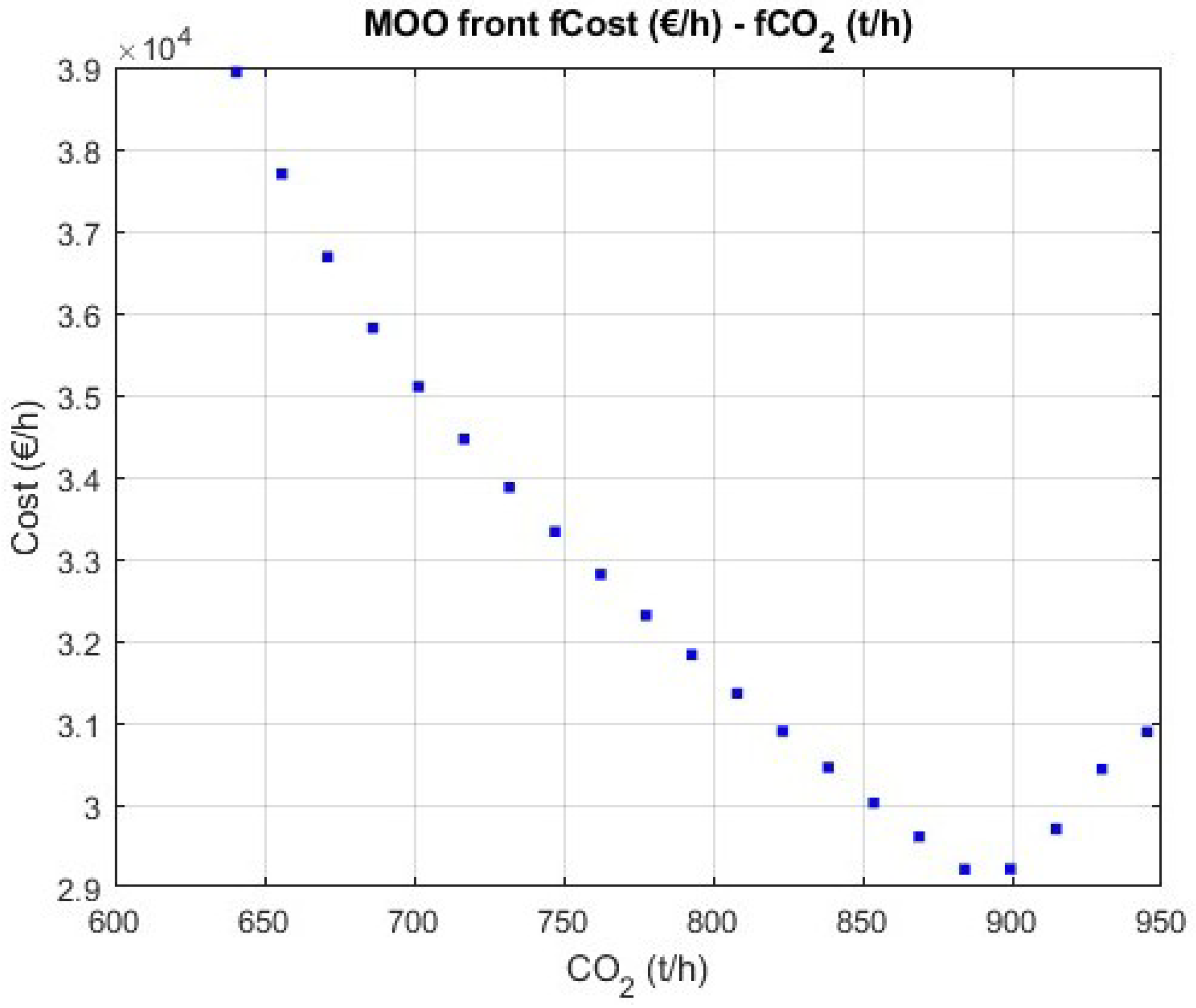
When exploring the extreme values of the objective functions, the system is capable of meeting demand through a range of generation mixes, resulting in cost values between EUR 28,976/h and 39,546/h and CO₂ emissions ranging from 640.59 t/h to 945.12 t/h. Figure 15 displays the multi-objective frontier without filtering out dominated solutions, allowing for the visualisation of the boundary values for the emissions function. The four points located in the bottom-right corner are not part of the Pareto front, as each can be outperformed by other solutions that offer both lower cost and lower emissions. Therefore, these points are considered to be dominated. Nevertheless, the rightmost point represents the highest level of CO₂ emissions the system can produce—945.12 t/h—which is taken as the upper bound for emissions.

The Pareto front establishes the base case to analyse how the optimal solutions vary when the actual power injected by the wind farms differs from the forecast.

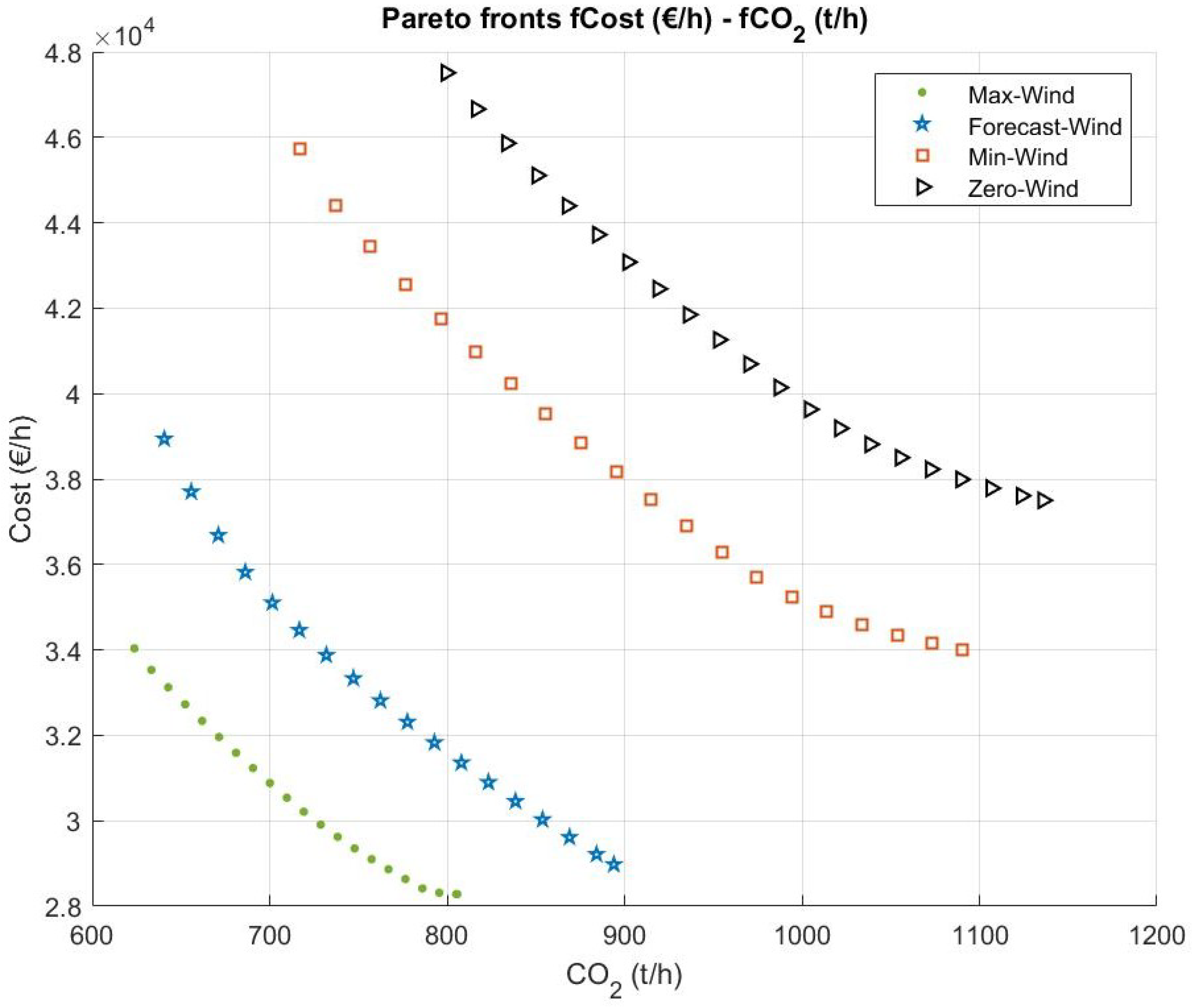
For each estimated wind farm, a series of 2000 points of random power deviations was generated following the kernel distributions adjusted in the previous section. Thus, 2000 random combinations of the six wind-farm powers that deviated from the estimated forecast were generated. The combinations that represented the maximum increase (Max-Wind) and decrease (Min-Wind) of total wind over the forecast were identified.

Figure 16 shows the Pareto fronts between the cost and CO₂ emission functions for four significant situations: maximum wind, forecast wind, minimum wind, and null wind. The ranges of costs and emissions along which the functions move change for each situation, increasing as the wind decreases, since wind can be interpreted as a decrease in demand at zero cost.

Next, using the estimated wind forecast curve as a reference, optimal-cost generation solutions were identified across 2000 variations in wind farm output, all constrained by total system emissions. Simulations were conducted to meet emission targets set at 25%, 50%, and 75% of the emissions range observed in the base case—specifically, 717, 793, and 869 t/h, respectively. In total, 6000 scenarios (2000 for each emission target) were simulated and solved.

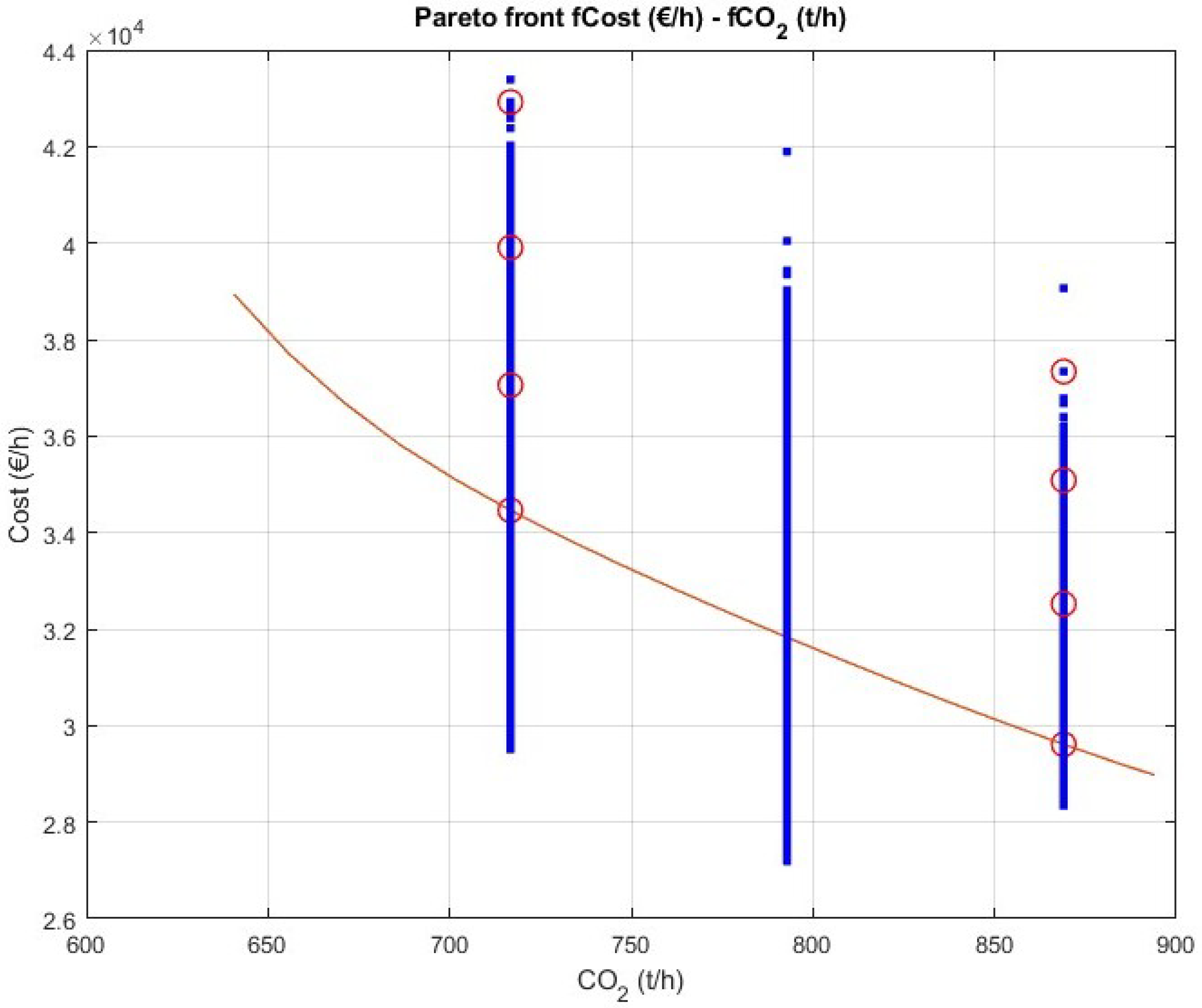
In Figure 17, the evolution of the Pareto Front base is depicted as a continuous curve. The vertical dispersion of points represents the optimal cost corresponding to a specific constraint on generated emissions across all studied scenarios of random wind deviations. Each group of vertically dispersed solutions comprises approximately 2000 points—slightly fewer in practice, as solutions failing to meet optimality convergence criteria were excluded. For emission constraints of 25% and 75%, four circled points are highlighted: the first lies on the Pareto baseline, while the three ascending vertical points represent optimal cost solutions as wind decreases, roughly segmented into the tertile bounds of the maximum negative wind deviation. The corresponding power-plant mix configurations for these points are analysed in subsequent sections.

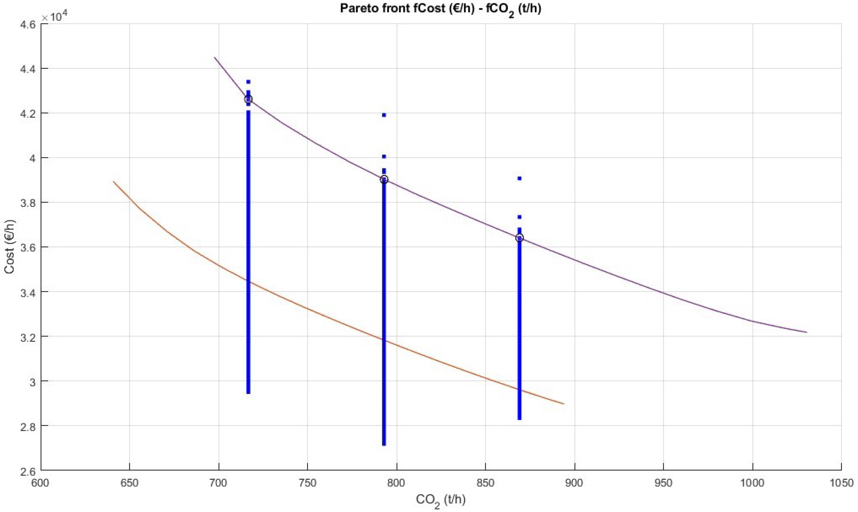
As an example, Figure 18 shows how the Pareto front changes as the wind deviates. The upper curve in the figure is the Pareto front for one of the 2000 random kernel deviations—in this case, for a situation accounting for a total wind power decrease of 139 MW. In the figure, circles indicate the new optimum solutions for the system still respecting 25%, 50%, and 75% of the emissions range.

The important fact is that it is possible to identify, for any deviation, the new optimal solutions for the system, satisfying any emission limit; therefore, it is possible to take corrective actions for the short-term dispatch strategy or for intraday or secondary/tertiary regulation market offers.

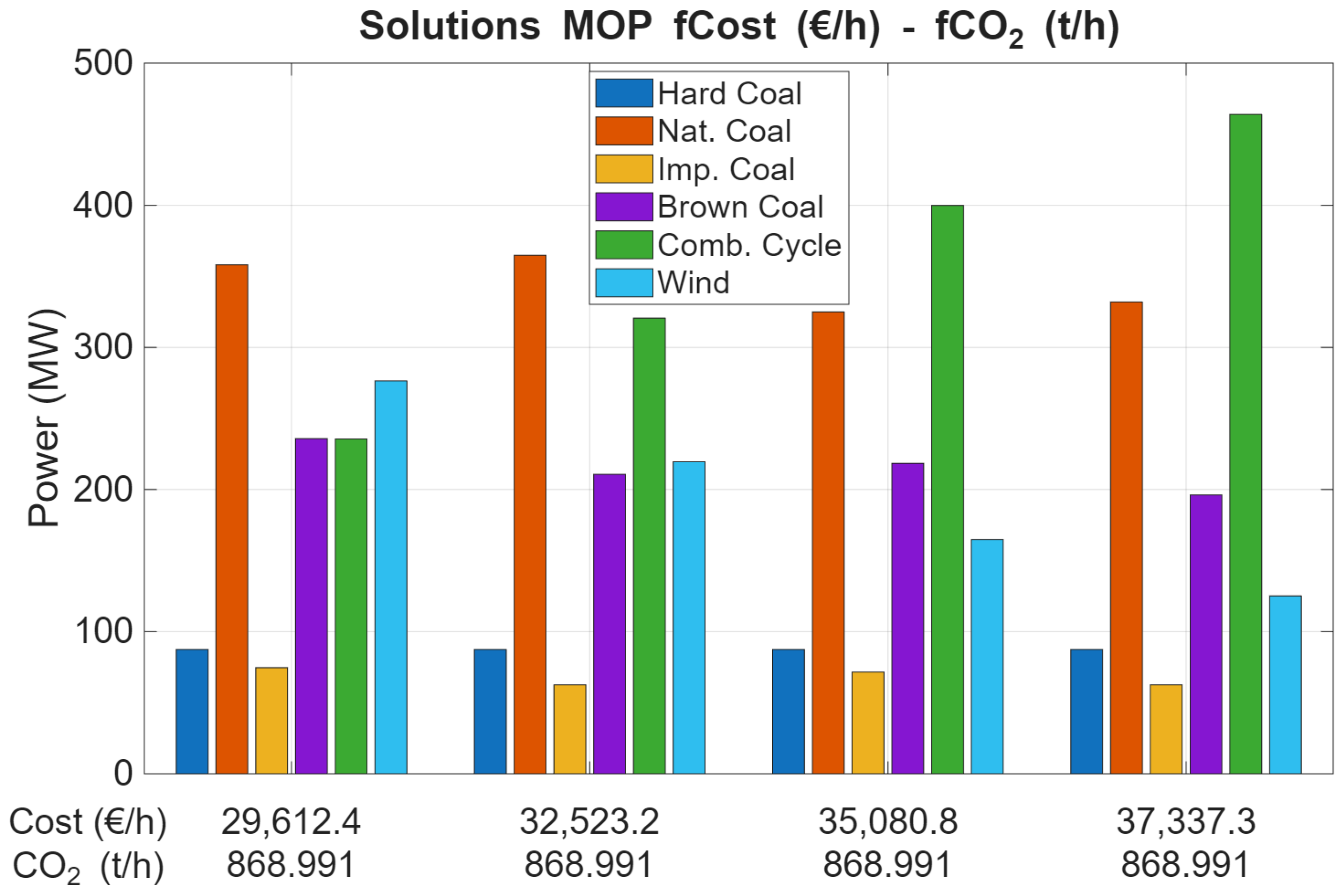
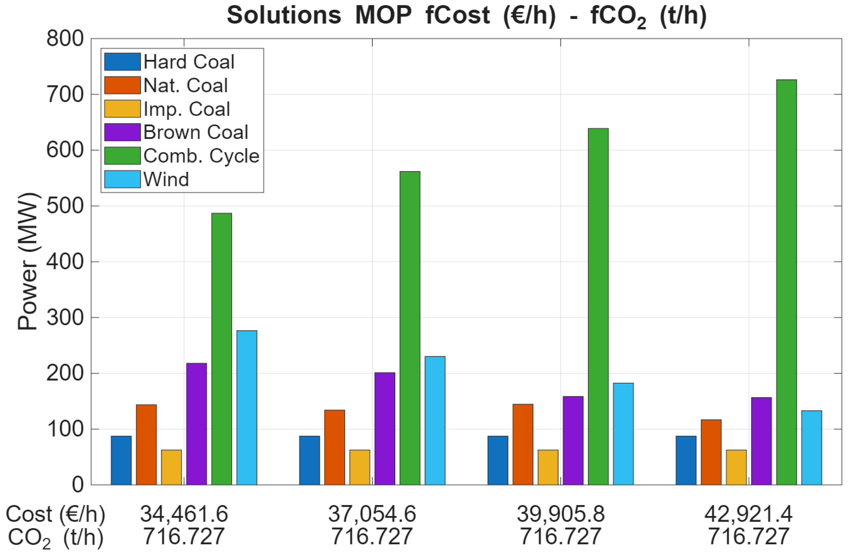
Figure 19 and Figure 20 illustrate how the optimal generation mix must change when wind generation deviates from its forecasted value while complying with certain emission limits. The points shown in Figure 19 and Figure 20 correspond to the circled solutions in Figure 17, representing emission ranges of 75% and 25%, respectively.

Environmental requirements are stricter in Figure 20, which corresponds to an emission limit of 716.7 t CO₂, compared to Figure 19 with 869 t CO₂. In both cases, it is evident that wind deviations lead to the substitution of coal with combined-cycle gas plants—more significantly under tighter emission constraints.

However, when comparing the two scenarios, the 75% CO₂ emission range allows for notable participation of coal units, particularly national hard coal and brown coal (Figure 19). This participation is greatly reduced when emissions are limited to 25% (Figure 20), where even under accurate wind forecasts, gas cycles must become the main producers. As shown in the figures, brown coal contributes more than other higher-rank coal-fired plants—perhaps surprisingly—because its fixed carbon content is relatively low. However, this situation would change if, for example, SO₂ emissions without flue-gas treatment were also considered.

This methodology enables the generating company or system operator to schedule the most cost-effective energy mix for the day-ahead market, considering forecasted wind resources while meeting environmental requirements. Furthermore, in the event of a significant and confirmed deviation in the upcoming hours, it allows the operator to analyse the short-term adjustments in the dispatchable generation power plants to maintain economic optimality while complying with the same environmental constraint. The algorithm computes and stores the corresponding solutions in the design space, simultaneously validating the feasibility of the power flow.

In this regard, an important factor to consider is the location of wind power generation and conventional power plants within the electrical network under study, since transmission constraints can alter the amount of power each plant must supply to compensate for wind deviations.

For instance, considering the transition depicted in Figure 17 from the first to the third point, if emissions are capped at 716.7 t CO₂ and wind generation drops from the forecasted 276.42 MW to 182.47 MW—a reduction of 93.95 MW—the corresponding generation profiles and optimal adjustments for each plant are detailed in

Table 4. Optimal adjustments for generations units.

Bus	Plant Type	Forecasted Wind Power Production [MW]	Production in the Deviated Scenario [MW]	Optimal Shift [MW]
1	CC	219.65	296.75	+77.10
2	H	87.50	87.50	0.00
3	IC	62.50	62.50	0.00
6	B	218.00	158.47	−59.53
8	NC	56.25	56.25	0.00
9	CC	267.30	342.10	+74.80
12	NC	87.40	88.27	+0.87
Multiple buses	Wind	276.42	182.47	−93.95 (deviation)

. These changes can be directly executed by the system operator within a dispatch-driven framework or offered in energy markets, such as secondary or tertiary regulation services.

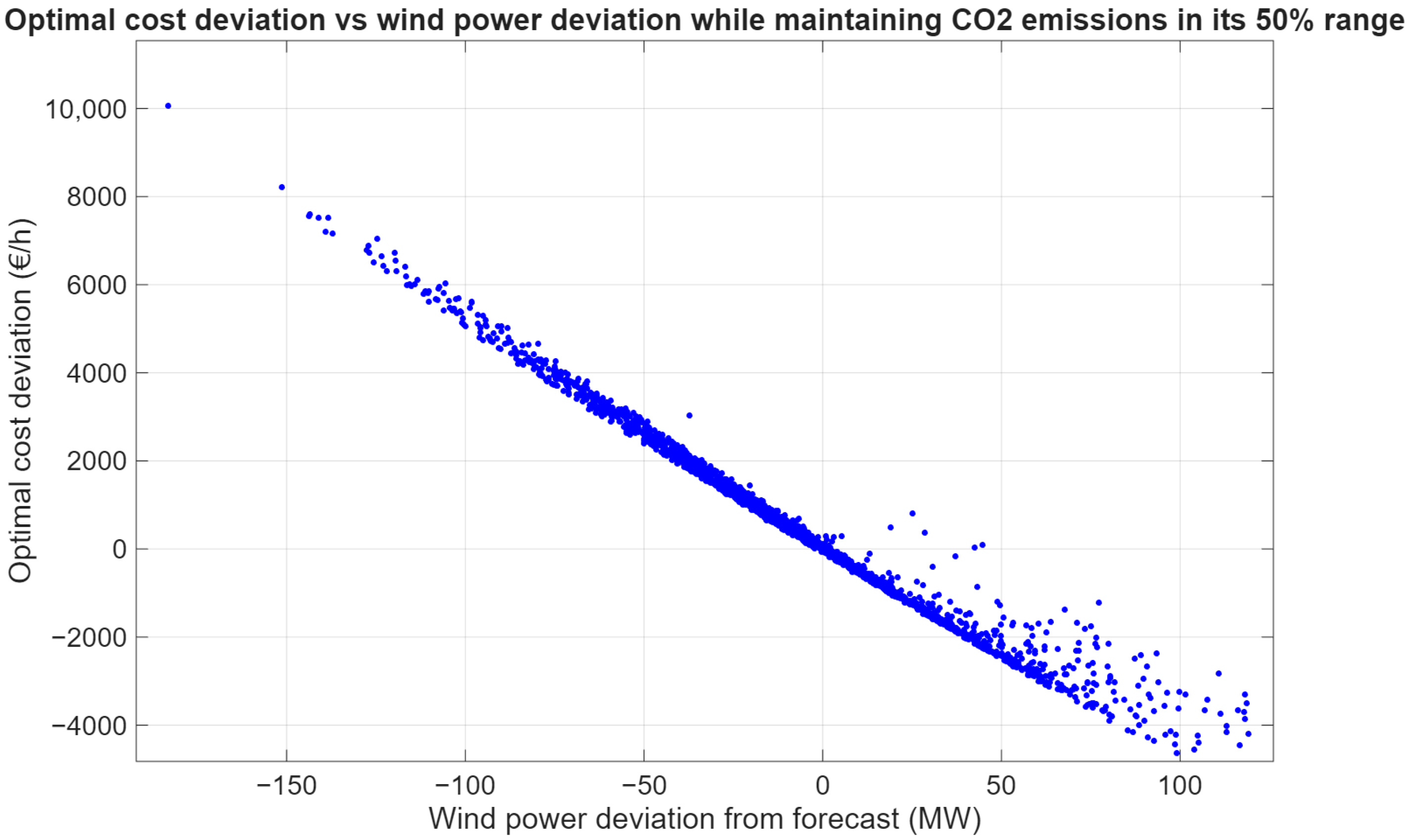
Finally, it is also possible to study and represent how the total optimal cost changes with wind-power deviations while maintaining a certain level of emissions, as shown in Figure 21 for 50% of the emission range in the baseline case.

The distributions of optimal costs around the value obtained in the base case, associated with the studied emissions, indicate that the mix of forecast errors committed in the studied wind farms has a strong influence and does not follow a homogeneous distribution around the value of the base case, as expected.

The simulation results in

Table 5. Summary of simulation results.

Emissions [pu]	Emissions [tCO2/h]	Pareto Cost Solution [k€/h]	Mean Real Cost [k€/h]	Standard Deviation [k€/h]
0.25	716.7	34.36	35.07	2.324
0.5	792.8	31.83	32.36	2.195
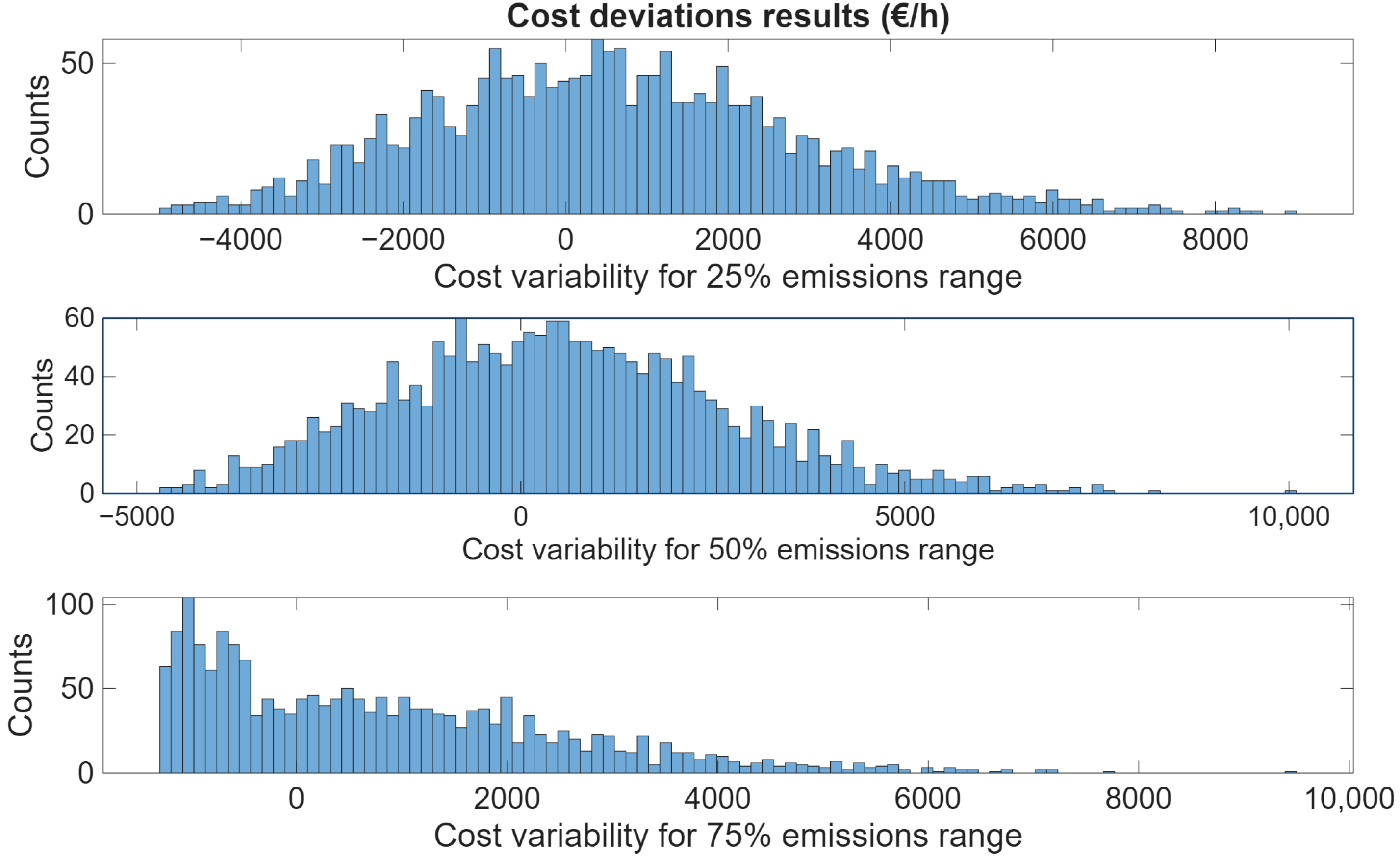
0.75	867.0	29.61	30.43	1.718

show that the average cost of actual power output exceeds the Pareto-estimated cost, suggesting that asymmetries in forecast errors lead to an average additional cost across the three analysed emission scenarios. For example, in the case of emissions at 0.75 pu, the average extra cost is approximately 2.7%. The distribution of wind prediction errors exhibits a negative bias, with a greater number of random cases falling below the forecast wind level than exceeding it across the 2000 simulated scenarios.

Figure 22 shows a summary of the histograms of the incremental costs, and it can be seen how the wind forecast errors are echoed to the generation costs. The variability of costs with respect to the base case follows different distributions depending on the emissions restriction.

For a 25% emission-range restriction, costs increase because combined-cycle power plants are the main players in offsetting wind-power deviations. In the case of the 50% emission-range constraint, average costs increase slightly less, as the system still has room to find intermediate solutions involving coal and combined-cycle participation.

However, the 75% emission scenario follows an atypical histogram, mainly due to the rigid constraint of producing exactly at that emission level. The asymmetry in this histogram is primarily explained by examining the positive wind deviations: several simulations with significant positive wind deviations failed to converge, as the thermal farm is unable to adapt to those emissions at a reduced share of total generation. When it does manage to adapt, higher costs sometimes result, since the system is forced to use plants with higher fixed carbon content, even if they are more expensive (e.g., national coal versus brown coal). For negative wind deviations, the behaviour is similar to the other scenarios.

8. Conclusions

The progressive integration of renewable energy sources into the power system represents a significant environmental advancement and contributes to reduced national energy dependence. This transition fosters a cleaner and more sustainable society. However, achieving environmental targets also requires the addressing of the specific characteristics of each renewable technology. The inherent uncertainty of wind and solar power—key drivers of the transformation in electricity generation—necessitates a thorough analysis of their impact on system operations and the additional costs they may incur.

This study identifies a computational approach to assess how wind variability influences decision making in conventional thermal generation. A multi-objective optimization framework was implemented, incorporating an AC optimal power flow model. The analysis reveals that prediction errors are not symmetrically distributed around the forecasted values, which may stem from limitations in forecasting methods and operational dynamics of wind farms. Statistical modelling of these errors using kernel density estimation enables the generation of random values that closely match the observed histograms.

The method presented in this study enables anticipation of potential wind forecast deviations relative to the prediction of the previous day, offering a valuable tool for operators managing a portfolio of generation units. It provides insight into the optimal generation strategies for each active plant that may need to be deployed in the short term should such deviations occur while ensuring compliance with a predefined emission limit—either set by the system operator or mandated by regulatory frameworks.

These optimal generation adjustments can be implemented through various mechanisms, depending on the local operational regime of the power system. They may be integrated into economic dispatch strategies or offered in ancillary service markets, such as secondary or tertiary reserves, or deviation management markets.

In this initial study, only thermal generation plants were considered. As a continuation of the work, hydraulic generation and energy storage systems, such as batteries, compressed air, or hydrogen storage, should be incorporated into optimization, as they may significantly modify how the electrical system is managed.