A Novel Fault Ranging Method for High-Voltage AC Transmission Lines Based on Attention-GRU and Modulus Amplitude Ratio

Abstract

Existing high-voltage alternating current (AC) transmission line fault ranging methods have several drawbacks, including weak transition resistance, a complicated feature extraction process, and difficult calibration of the travelling wave head. To address these issues, a single-end fault ranging method for high-voltage AC transmission lines based on Attention-GRU and modulus amplitude ratio is proposed. Firstly, based on the travelling wave dispersion characteristics, an approximate formula is derived between the fault distance of the high-voltage AC transmission line and the amplitude ratio of the sum of the initial transient voltage travelling wave modes 1 and 2 and the mode 0 components at the ranging location. This shows that a definite nonlinear mapping relationship exists between the two. Secondly, the Attention-GRU is constructed using the multiscale wavelet modal maxima ratio between the sum of the initial transient voltage travelling wave mode 1 and 2 components and the mode 0 component as the input eigenquantities and the fault distance as the output quantity. The fault distance is then calculated using the Attention-GRU and the modal amplitude ratio. The Attention-GRU neural network fault ranging model is then constructed using the distance as the output quantity. After training is completed, the fault feature quantities obtained from the measurement points are inputted into the Attention-GRU model to achieve the purpose of fault ranging. The ranging ability of this model is then compared with that of other neural network models. A large number of simulations verify that the proposed method has high ranging accuracy and that the ranging capability is not affected by the fault type, transition resistance or the initial phase angle of the fault.

1. Introduction

As the economy continues to develop and the industrialisation process accelerates, the social demand for electricity continues to rise. Transmission lines are the core channel for the long-distance transmission of electricity, so ensuring their safe and stable operation is critical to the entire power system. If a fault occurs on a high-voltage AC transmission line and cannot be quickly and accurately located, the scope of power supply interruption will expand and recovery time will be prolonged [1]. This will have a serious impact on social production, life and economic development. Therefore, studying fault ranging in high-voltage AC transmission lines is important for quickly and accurately determining the location of faults, which helps to shorten outage times and improve the reliability and stability of power grid operation.

Currently, many studies have been conducted on the fault ranging of high-voltage AC transmission lines, with the most common methods being the travelling wave ranging method and the fault analysis method. The travelling wave ranging method extracts the travelling wave of the fault that arrives at the moment of the measuring device and constructs the corresponding ranging equation to determine the location of the fault [2]. Its theoretical principle is simple and it is widely used in engineering practice. Among them, double-ended travelling wave ranging technology has attracted much attention because of its high measurement accuracy, but it is necessary to ensure the strict time synchronisation of the equipment at both ends, and the cost of the equipment is high; single-ended travelling wave ranging method is mainly faced with the identification of the reflected wave from the fault point and the opposite end of the identification of the problem, especially in the case of faults occurring in the middle of the line or near the end of the line, the travelling wave signals are prone to produce overlapping interference, which affects the accuracy of the localization. In addition, the travelling wave method is highly dependent on the accuracy of wavehead identification and sampling frequency, which further limits its practical performance. In contrast, the fault analysis method is one of the effective ways to solve the transmission line fault ranging problem by measuring the electrical quantities at the end and constructing the fault localization criterion by combining the system structure and parameters, which has lower requirements on the measurement equipment and wider scope of application.

Addressing the issue of wavehead calibration, the literature [3] presents a fault ranging method based on time-frequency analysis. This method has a straightforward fault localisation process and effectively mitigates the impact of harsh environmental conditions and wavehead calibration errors on localisation results. Furthermore, it demonstrates high fault tolerance. Literature [4] uses the Teager energy operator to extract the mutation characteristics of high-frequency modal components and establish the identification principle of a multi-branch line. This accurately calibrates the arrival time of the travelling wave head, improving the accuracy of fault location. Literature [5] proposes a hybrid line fault section identification and localisation method based on the amplitude ratio of the faulty travelling wave. This method corrects double-ended ranging by introducing a position compensation factor, and realises efficient travelling wave head detection by combining with symmetric mode decomposition of the extremum point. Literature [6] uses variational mode decomposition (VMD) combined with the Northern Goshawk optimisation algorithm (NGO) for wavehead calibration, accurately calculating the fault location using the two-end travelling wave fault detection formula. While the above methods demonstrate strong adaptability, they generally exhibit high computational complexity, which restricts their practical application efficiency.

In response to the issue of selecting wave speeds, the literature [7] proposes a single-ended travelling wave ranging method based on optimised variational mode decomposition. This method uses the eigenmode function to estimate wave speeds. However, the accuracy of this method is difficult to guarantee when travelling wave attenuation is significant. Literature [8] uses robust local mean decomposition, the Teager energy operator, and the incremental difference ratio for wave speed detection. Fault localisation is achieved by gradually narrowing down the scope of the fault region. Literature [9] proposes a fault localisation method for T-type AC/DC hybrid transmission lines based on modal time difference and wave speed normalisation. This method is unaffected by travelling wave speed, but the calculations are more complicated.

In recent years, advances in artificial intelligence technology have generated new approaches to fault ranging research. Literature [10] used wavelet packet energy entropy to extract fault features and then used the obtained high- and low-frequency components as training samples for different DBN models. The outputs of each model were then superimposed to obtain the final fault localisation results. Literature [11] proposed a single-ended fault localisation method based on an S-transform combined with feature energy and an improved CNN-GRU neural network model, which offers high localisation accuracy and good robustness. Literature [12] uses an improved adaptive noise complete ensemble empirical mode decomposition (ICEEMDAN) to analyse signals, with the root mean square error of the ConvGRU model training acting as the adaptation value. The model’s internal parameters are optimised using a continuous averaging algorithm to produce a combined fault location model. While this model demonstrates good localisation accuracy and moderate interference resistance, it exhibits significant positioning errors at low sampling frequencies. Literature [13] provides a thorough investigation of Long Short-Term Memory (LSTM) units and their variants, examining their ability to address long-term dependency issues. Literature [14] proposes that BP neural networks possess strong self-learning, adaptive and generalisation capabilities. Their tendency to converge to local optima can be mitigated through genetic algorithm optimisation. Such AI-based ranging methods offer significant advantages in terms of enhancing ranging accuracy. However, they typically require large sample datasets, exhibit high computational complexity and demand stringent technical implementation. Furthermore, their optimisation outcomes are susceptible to initial parameter settings [15].

In order to address these challenges, this paper proposes a single-ended fault location method for high-voltage AC transmission lines. This method is based on Attention-GRU and the modulus-to-amplitude ratio. This method only requires the initial transient voltage travelling wavefront signal to be acquired at the distance measurement device, thus resolving the issue of identifying the reflecting wavefront in single-ended travelling wave methods. Only the initial transient voltage travelling wavefront amplitude needs to be extracted, bypassing the problem of inaccurate wavefront arrival time calibration caused by travelling wave dispersion characteristics. Furthermore, it eliminates the requirement for travelling wave velocity calculation, bypassing the accuracy issues associated with wave velocity estimation in single-ended travelling wave methods. The wavelet mode maximum ratio between the sum of the initial transient voltage travelling wave mode 1 and mode 2 components collected at the distance measurement device and the mode 0 component is treated as the sample set. This is input into the Attention-GRU neural network distance measurement model to fit the nonlinear mapping relationship between the fault distance and the amplitude ratio between the sum of the voltage mode 1 and mode 2 components and the mode 0 component.

The distance measurement method described herein fundamentally differs from traditional travelling wave methods at its core. While conventional approaches focus on employing various technical means to circumvent or suppress the interference caused by travelling wave dispersion effects on wavefront identification, this paper achieves a paradigm shift by deeply analysing and leveraging the dispersion characteristics of travelling waves. It transforms these characteristics into effective features for measuring fault distances, thereby transitioning from interference avoidance to utilisation of the underlying mechanism. This approach offers a novel perspective for fault location in high-voltage AC transmission lines.

2. Materials and Methods

2.1. Asymmetrical Ground Fault Ranging Principles

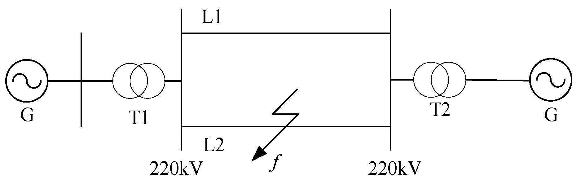
The topology of the 220 kV high-voltage AC transmission line is shown in Figure 1. The parameters of high-voltage AC transmission lines are shown in

Table 1. Parameters of high-voltage ac transmission lines.

Ordinal Component	Resistance (Ω/km)	Reactance (Ω/km)	Conductivity (S/km)	Nanoelectricity (S/km)
Positive/Negative sequence	0.0345	0.423	1 × 10−10	2.707 × 10−6
Zero sequence	0.181	1.452	1 × 10−10	1.934 × 10−6

. The total length of the high-voltage AC transmission line is 200 km, and the fault ranging device is installed at the substation, and the sampling frequency is set to 1 MHz.

Asymmetric ground faults in high-voltage AC transmission lines include single-phase and two-phase ground faults. When a ground fault occurs at point f, the transient travelling wave process of the fault is equivalent to the superposition theorem. This is equivalent to suddenly adding a voltage of the same size but opposite direction to the pre-fault voltage at the fault point [16].

The first three-phase voltages at the first end of a high-voltage AC transmission line before a fault are

$$\left\{\begin{array}{l}{u}_A(t)=\sqrt{2}U\cos (\omega t)\\ u_{\mathrm{B}}(t)=\sqrt{2}U\cos (\omega t-{120}^{\circ })\\ u_{\mathrm{C}}(t)=\sqrt{2}U\cos (\omega t+{120}^{\circ })\end{array}\right.$$

(1)

Under normal operating conditions, the relationship between the voltage at a given distance from the first end of a high-voltage AC transmission line and the voltage at the first end of the line before a fault occurs is as follows:

$$\left\{\begin{array}{l}{u}_{Ax}(t)=u_A(t){\mathrm{e}}^{-{\displaystyle \frac{r_0}{2z^x}}}=\sqrt{2}U\cos (\omega t){\mathrm{e}}^{-{\displaystyle \frac{r_0}{2z^x}}}\\ u_{\mathrm{Bx}}(t)=u_{\mathrm{B}}(t){\mathrm{e}}^{-{\displaystyle \frac{r_0}{2z^x}}}=\sqrt{2}U\cos (\omega t-{120}^{\circ }){\mathrm{e}}^{-{\displaystyle \frac{r_0}{2z^x}}}\\ u_{\mathrm{Cx}}(t)=u_{\mathrm{C}}(t){\mathrm{e}}^{-{\displaystyle \frac{r_0}{2z^x}}}=\sqrt{2}U\cos (\omega t+{120}^{\circ }){\mathrm{e}}^{-{\displaystyle \frac{r_0}{2z^x}}}\end{array}\right.$$

(2)

where $u_{Ax}\left(t\right)$ is the distance from the first end of the $x$ phase A voltage line; $u_{Bx}\left(t\right)$ is the distance from the first end of the $x$ phase B voltage line; $u_{Cx}\left(t\right)$ is the distance from the first end of the $x$ phase C voltage line; $r_0$ is the unit length of the wire resistance; and $z$ is the line wave impedance.

2.2. Single-Phase Ground Fault Ranging Principle

Using phase A ground fault as an example, the initial transient voltage travelling wave of each modulus at the fault point is determined by considering the effect of transition resistance:

$$\left\{\begin{array}{l}\begin{array}{c}{u}_{f0}^{(1)}=-{\displaystyle \frac{Z_0}{Z_0+Z_1+Z_2+6R_f}}{u}_{\mathrm{Ax}}(t)=\\ -{\displaystyle \frac{Z_0\sqrt{2}U\cos (\omega t){\mathrm{e}}^{-\frac{r_0}{2z^x}}}{Z_0+Z_1+Z_2+6R_f}}\end{array}\\ \begin{array}{c}{u}_{f1}^{(1)}=-{\displaystyle \frac{Z_1}{Z_0+Z_1+Z_2+6R_f}}{u}_{Ax}(t)=\\ -{\displaystyle \frac{Z_1\sqrt{2}U\cos (\omega t){\mathrm{e}}^{-\frac{r_0}{2z^x}}}{Z_0+Z_1+Z_2+6R_f}}\end{array}\\ \begin{array}{c}{u}_{f2}^{(1)}=-{\displaystyle \frac{Z_2}{Z_0+Z_1+Z_2+6R_f}}{u}_{\mathrm{Ax}}(t)=\\ -{\displaystyle \frac{Z_2\sqrt{2}U\cos (\omega t){\mathrm{e}}^{-\frac{r_0}{2z^x}}}{Z_0+Z_1+Z_2+6R_f}}\end{array}\end{array}\right.$$

(3)

where $u_{f0}^{\left(1\right)}, u_{f1}^{\left(1\right)}, u_{f2}^{\left(1\right)}$ are the initial transient voltage traveling wave 0-mode, 1-mode, 2-mode components at the fault point A phase ground fault; $Z_0, Z_1, Z_2$ are the 0-mode, 1-mode, 2-mode wave impedance of the high-voltage AC transmission line.

The propagation function $A_j$ of a high-voltage AC transmission line with modulus propagation coefficient ${\gamma }_j$ and length $x$ in the line is as follows [17]:

$$A_j(\mathrm{j}\omega )={\displaystyle \frac{u_j(\mathrm{j}\omega )}{u_f(\mathrm{j}\omega )}}={\mathrm{e}}^{-{\gamma }_{j}x}$$

(4)

$${\gamma }_j=\sqrt{(R_j+\mathrm{j}\omega L_j)\times \mathrm{j}\omega K_j}={\alpha }_j+j{\beta }_j$$

(5)

where $j=0, j=1, j=2$, respectively, for the 0 mode, 1 mode, 2 mode; $\omega$ for the system angular frequency; $u_j\left(j\omega \right), u_{fj}\left(j\omega \right)$, respectively, for the distance measurement, the fault point modal voltage; $R_j, L_j, K_j$, respectively, for the unit length of the line modal resistance, inductance, capacitance; ${\alpha }_j$ for the line modal attenuation constant, determining the amplitude of the propagation of travelling wave attenuation characteristics; ${\beta }_j$ for the line modal phase coefficient, determining the phase lag characteristics of the propagation of travelling wave. Uniformly transposed three-phase line in the 1-mode component and the 2-mode component of the parameters are equal, can be regarded as ${\gamma }_1={\gamma }_2$, from Equation (4) can be launched single-phase ground fault line first end of the initial transient voltage ranging at the initial transient voltage travelling wave modulus and fault initial transient voltage travelling wave modulus of the relationship between the point is

$$\begin{array}{l}{u}_0^{(1)}\left(\mathrm{j}\omega \right)={\mathrm{e}}^{-{\gamma }_{0}x}{u}_{f0}^{(1)}\left(\mathrm{j}\omega \right)=\\ -{\displaystyle \frac{Z_0}{Z_0+Z_1+Z_2+6R_f}}{u}_{Ax}(t){\mathrm{e}}^{-{\gamma }_{0}x}=\\ -{\displaystyle \frac{Z_0\sqrt{2}U\cos (\omega t)}{Z_0+Z_1+Z_2+6R_f}}{\mathrm{e}}^{-{\gamma }_{0}x}{\mathrm{e}}^{-{\displaystyle \frac{r_0}{2z^x}}}\end{array}$$

(6)

$$\begin{array}{l}{u}_1^{(1)}\left(\mathrm{j}\omega \right)={\mathrm{e}}^{-{\gamma }_{1}x}{u}_{f1}^{(1)}\left(\mathrm{j}\omega \right)=\\ -{\displaystyle \frac{Z_1}{Z_0+Z_1+Z_2+6R_f}}{u}_{Ax}(t){\mathrm{e}}^{-{\gamma }_{1}x}=\\ -{\displaystyle \frac{Z_1\sqrt{2}U\cos (\omega t)}{Z_0+Z_1+Z_2+6R_f}}{\mathrm{e}}^{-{\gamma }_{1}x}{\mathrm{e}}^{-{\displaystyle \frac{r_0}{2z^x}}}\end{array}$$

(7)

$$\begin{array}{l}{u}_2^{(1)}\left(\mathrm{j}\omega \right)={\mathrm{e}}^{-{\gamma }_{2}x}{u}_{f2}^{(1)}\left(\mathrm{j}\omega \right)=\\ -{\displaystyle \frac{Z_2}{Z_0+Z_1+Z_2+6R_f}}{u}_{Ax}(t){\mathrm{e}}^{-{\gamma }_{2}x}=\\ -{\displaystyle \frac{Z_2\sqrt{2}U\cos (\omega t)}{Z_0+Z_1+Z_2+6R_f}}{\mathrm{e}}^{-{\gamma }_{1}x}{\mathrm{e}}^{-{\displaystyle \frac{r_0}{2z^x}}}\end{array}$$

(8)

where $u_0^{\left(1\right)}\left(j\omega \right), u_1^{\left(1\right)}\left(j\omega \right), u_2^{\left(1\right)}\left(j\omega \right)$ for the range at the 0-mode, 1-mode, 2-mode voltage; ${\gamma }_0, {\gamma }_1, {\gamma }_2$ for the 0-mode, 1-mode, 2-mode voltage travelling wave propagation coefficient. From Equations (6)–(8), the following can be obtained:

$$\begin{array}{l}{\displaystyle \frac{u_1^{(1)}\left(\mathrm{j}\omega \right)+u_2^{(1)}\left(\mathrm{j}\omega \right)}{u_0^{(1)}\left(\mathrm{j}\omega \right)}}=\\ {\displaystyle \frac{u_{\mathrm{A}x}\left(t\right)\left({\mathrm{e}}^{-{\gamma }_{1}x}{Z}_1+{\mathrm{e}}^{-{\gamma }_{2}x}{Z}_2\right)}{u_{\mathrm{A}x}\left(t\right){\mathrm{e}}^{-{\gamma }_{0}x}{Z}_0}}=\\ {\displaystyle \frac{(Z_1+Z_2)}{Z_0}}{\mathrm{e}}^{({\gamma }_0-{\gamma }_1)x}\end{array}$$

(9)

Taking the amplitude on both sides of Equation (9) yields the following result:

$$\left|{\displaystyle \frac{u_1^{(1)}\left(\mathrm{j}\omega \right)+u_2^{(1)}\left(\mathrm{j}\omega \right)}{u_0^{(1)}\left(\mathrm{j}\omega \right)}}\right|=\left|{\displaystyle \frac{Z_1+Z_2}{Z_0}}\right|{\mathrm{e}}^{({\alpha }_0-{\alpha }_1)x}$$

(10)

Let $\left|{\displaystyle \frac{Z_1+Z_2}{Z_0}}\right|={\displaystyle \frac{1}{k_1}}$, $u_{12}^{\left(1\right)}\left(j\omega \right)=u_1^{\left(1\right)}\left(j\omega \right)+u_2^{\left(1\right)}\left(j\omega \right)$, when the structure and parameters of the high-voltage AC transmission line are determined, $Z_0, Z_1, Z_2, {\alpha }_0, {\alpha }_1$ are constants, the following can be obtained:

$$x={\displaystyle \frac{1}{{\alpha }_0-{\alpha }_1}}\ln \left(k_1{\displaystyle \frac{\mid u_{12}^{(1)}\left(\mathrm{j}\omega \right)\mid }{\mid u_0^{(1)}\left(\mathrm{j}\omega \right)\mid }}\right)$$

(11)

Equation (11) indicates that, in the event of a single-phase ground fault, the fault distance is related to the amplitude ratio between the sum of the 1-mode and 2-mode components of the initial transient voltage travelling wave and the 0-mode component. This ratio is unaffected by the transition resistance and the initial phase angle of the fault.

2.3. Two-Phase Ground Fault Ranging Principle

Taking phase B and C ground fault as an example, considering the effect of transition resistance [18], the initial transient voltage travelling wave of each modulus at the fault point can be deduced by the same reason:

$$\begin{array}{l}{u}_{f0}^{\left(1,1\right)}={\displaystyle \frac{Z_0}{Z_m}}{u}_{Ax}\left(t\right)=\\ {\displaystyle \frac{Z_0}{Z_m}}\sqrt{2}U\cos \left(\omega t\right)e^{-{\displaystyle \frac{r_0}{2z^x}}}\end{array}$$

(12)

$$\begin{array}{l}{u}_{f1}^{\left(1,1\right)}={\displaystyle \frac{Z_0+2Z_1}{3Z_1\times Z_m}}{u}_{Bx}\left(t\right)+{\displaystyle \frac{Z_1-Z_0}{3Z_1\times Z_m}}{u}_{Cx}\left(t\right)=\\ {\displaystyle \frac{Z_0+2Z_1}{3Z_1\times Z_m}}\sqrt{2}U\cos \left(\omega t-{120}^{°}\right)e^{-{\displaystyle \frac{r_0}{2z^x}}}+\\ {\displaystyle \frac{Z_1-Z_0}{3Z_1\times Z_m}}\sqrt{2}U\cos \left(\omega t+{120}^{°}\right)e^{-{\displaystyle \frac{r_0}{2z^x}}}\end{array}$$

(13)

$$\begin{array}{l}{u}_{f2}^{\left(1,1\right)}={\displaystyle \frac{Z_1-Z_0}{3Z_1\times Z_m}}{u}_{Bx}\left(t\right)+{\displaystyle \frac{Z_0+2Z_1}{3Z_1\times Z_m}}{u}_{Cx}\left(t\right)=\\ {\displaystyle \frac{Z_1-Z_0}{3Z_1\times Z_m}}\sqrt{2}U\cos \left(\omega t-{120}^{°}\right)e^{-{\displaystyle \frac{r_0}{2z^x}}}+\\ {\displaystyle \frac{Z_0+2Z_1}{3Z_1\times Z_m}}\sqrt{2}U\cos \left(\omega t+{120}^{°}\right)e^{-{\displaystyle \frac{r_0}{2z^x}}}\end{array}$$

(14)

where $Z_m=2Z_0+Z_1+12R_f$; $u_{f0}^{\left(1,1\right)}, u_{f1}^{\left(1,1\right)}, u_{f2}^{\left(1,1\right)}$ are the initial transient voltage travelling wave 0-mode, 1-mode and 2-mode components at the fault point when phases B and C are connected to ground, respectively.

From Equation (4), the relationship between the initial transient voltage travelling wave modulus at the first end of the line ranging and the initial transient voltage travelling wave modulus at the point of fault can be introduced in the case of two-phase ground fault [19]:

$$\begin{array}{l}{u}_0^{(1,1)}\left(\mathrm{j}\omega \right)={\mathrm{e}}^{-{\gamma }_{0}x}{u}_{f0}^{(1,1)}\left(\begin{array}{c}\mathrm{j}\omega \end{array}\right)=\\ {\mathrm{e}}^{-{\gamma }_{0}x}{\displaystyle \frac{Z_0}{Z_{\mathrm{m}}}}{u}_{\mathrm{A}x}(t)=\\ {\displaystyle \frac{Z_0}{Z_{\mathrm{m}}}}\sqrt{2}U\cos (\omega t){\mathrm{e}}^{-{\gamma }_{0}x}{\mathrm{e}}^{-{\displaystyle \frac{r_0}{2z^x}}}\end{array}$$

(15)

$$\begin{array}{l}{u}_1^{(1,1)}\left(\mathrm{j}\omega \right)={\mathrm{e}}^{-{\gamma }_{1}x}{u}_{f1}^{(1,1)}\left(\mathrm{j}\omega \right)={\mathrm{e}}^{-{\gamma }_{1}x}{\mathrm{e}}^{-{\displaystyle \frac{r_0}{2z^x}}}\\ \left({\displaystyle \frac{Z_0+2Z_1}{3Z_1\times Z_m}}{u}_{Bx}(t)+{\displaystyle \frac{Z_1-Z_0}{3Z_1\times Z_m}}{u}_{Cx}(t)\right)\\ =\left({\displaystyle \frac{Z_0+2Z_1}{3Z_1\times Z_m}}\sqrt{2}U\cos (\omega t-{120}^{\circ })+\right.\\ \left.{\displaystyle \frac{Z_1-Z_0}{3Z_1\times Z_{\mathrm{m}}}}\sqrt{2}U\cos (\omega t+{120}^{\circ })\right){\mathrm{e}}^{-{\gamma }_{1}x}{\mathrm{e}}^{-{\displaystyle \frac{r_0}{2z^x}}}\end{array}$$

(16)

$$\begin{array}{l}{u}_2^{(1,1)}\left(\mathrm{j}\omega \right)={\mathrm{e}}^{-{\gamma }_{2}x}{u}_{f2}^{(1,1)}\left(\mathrm{j}\omega \right)\\ ={\mathrm{e}}^{-{\gamma }_{1}x}{u}_{f2}^{(1,1)}\left(\mathrm{j}\omega \right)={\mathrm{e}}^{-{\gamma }_{1}x}{\mathrm{e}}^{-{\displaystyle \frac{r_0}{2z^x}}}\\ \left({\displaystyle \frac{Z_1-Z_0}{3Z_1\times Z_m}}{u}_{Bx}(t)+{\displaystyle \frac{Z_0+2Z_1}{3Z_1\times Z_m}}{u}_{Cx}(t)\right)\\ =\left({\displaystyle \frac{Z_1-Z_0}{3Z_1\times Z_m}}\sqrt{2}U\cos (\omega t-{120}^{\circ })+\right.\\ \left.{\displaystyle \frac{Z_0+2Z_1}{3Z_1\times Z_m}}\sqrt{2}U\cos (\omega t+{120}^{\circ })\right){\mathrm{e}}^{-{\gamma }_{1}x}{\mathrm{e}}^{-{\displaystyle \frac{r_0}{2z^x}}}\end{array}$$

(17)

It can be obtained from Equation (13) to Equation (15):

$$\begin{array}{l}{\displaystyle \frac{u_1^{(1,1)}\left(\mathrm{j}\omega \right)+u_2^{(1,1)}\left(\mathrm{j}\omega \right)}{u_0^{(1,1)}\left(\mathrm{j}\omega \right)}}=\\ ={\displaystyle \frac{\left(\frac{3Z_1}{3Z_1\times Z_m}{u}_{Bx}(t)+\frac{3Z_1}{3Z_1\times Z_m}{u}_{Cx}(t)\right){\mathrm{e}}^{-{\gamma }_{1}x}}{\frac{Z_0}{Z_m}{u}_{Ax}(t){\mathrm{e}}^{-{\gamma }_{0}x}}}\\ ={\displaystyle \frac{\cos (\omega t-{120}^{\circ })+\cos (\omega t+{120}^{\circ })}{Z_0\cos (\omega t)}}{\mathrm{e}}^{({\gamma }_0-{\gamma }_1)x}\\ =-{\displaystyle \frac{1}{Z_0}}{\mathrm{e}}^{({\gamma }_0-{\gamma }_1)x}\end{array}$$

(18)

Taking the amplitude on both sides of Equation (18) yields

$$\left|{\displaystyle \frac{u_1^{(1,1)}\left(\mathrm{j}\omega \right)+u_2^{(1,1)}\left(\mathrm{j}\omega \right)}{u_0^{(1,1)}\left(\mathrm{j}\omega \right)}}\right|=\left|{\displaystyle \frac{1}{Z_0}}\right|{\mathrm{e}}^{({\alpha }_0-{\alpha }_1)x}$$

(19)

Let $\left|{\displaystyle \frac{1}{Z_0}}\right|={\displaystyle \frac{1}{k_2}}$, $u_{12}^{(1,1)}\left(\mathrm{j}\omega \right)=u_1^{(1,1)}\left(\mathrm{j}\omega \right)+u_2^{(1,1)}\left(\mathrm{j}\omega \right)$, when the structure and parameters of the high voltage AC transmission line are determined, $Z_0, {\alpha }_0, {\alpha }_1$ are constants, the following can be obtained:

$$x={\displaystyle \frac{1}{{\alpha }_0-{\alpha }_1}}\ln \left(k_2{\displaystyle \frac{|u_{12}^{(1,1)}(\mathrm{j}\omega )|}{|u_0^{(1,1)}(\mathrm{j}\omega )|}}\right)$$

(20)

Equation (20) shows that, in the event of a two-phase ground fault, the fault distance is related to the amplitude ratio between the sum of the 1-mode and 2-mode components of the initial transient voltage travelling wave and the 0-mode component. Therefore, the inductive derivation of Equations (11) and (20) can be obtained for an asymmetrical ground fault in a high-voltage AC transmission line [18]:

$$x={\displaystyle \frac{1}{{\alpha }_0-{\alpha }_1}}\ln \left(k_{\mathrm{n}}{\displaystyle \frac{\mid u_{12}(\mathrm{j}\omega )\mid }{\mid u_0(\mathrm{j}\omega )\mid }}\right)$$

(21)

where $u_{12}\left(j\omega \right), u_0\left(j\omega \right)$ are the sum of 1-mode and 2-mode components of the initial transient voltage at the range, and the 0-mode component, respectively; $k_n$ is a constant, related to the type of asymmetrical ground fault.

A zero-sequence component exists only during ground faults, not during phase-to-phase faults. Thus, Equation (21) becomes invalid for non-ground faults, rendering this method unsuitable for phase-to-phase faults. Equation (21) enables distance measurement for asymmetric ground faults—which occur frequently yet exhibit elusive characteristics—without being affected by the initial phase angle or transition resistance. It fundamentally meets the distance measurement requirements for asymmetric ground faults in high-voltage AC transmission lines.

3. Effect of Transition Resistance and Fault Initial Phase Angle

3.1. Effect of Transition Resistance on Ranging Effectiveness

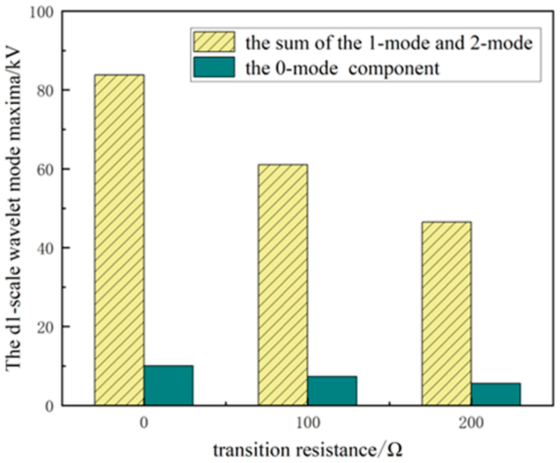
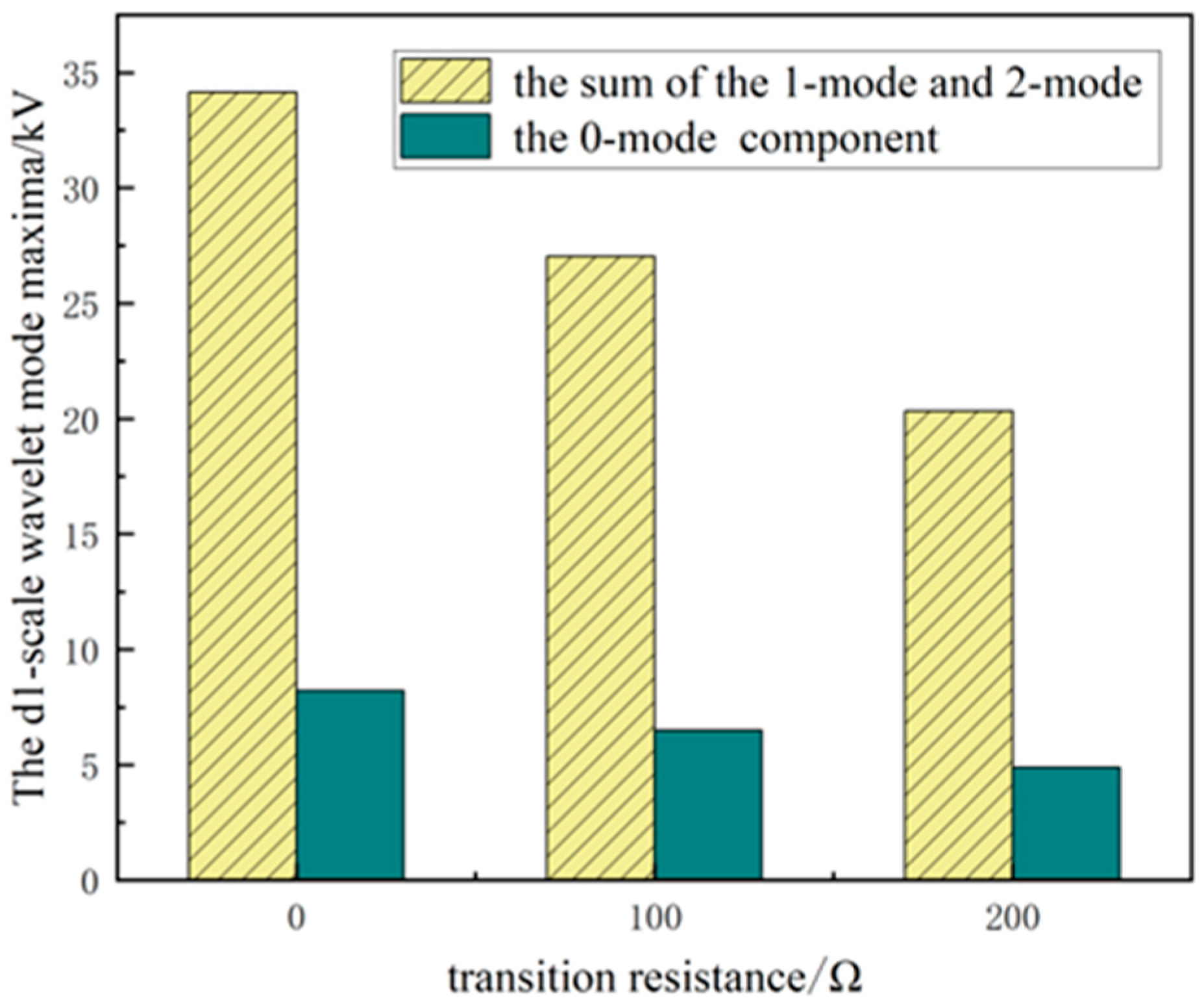
The frequency-dependent characteristics of high-voltage AC transmission lines show that the wave impedance of the sum of the 1-mode and 2-mode components, as well as that of the 0-mode component, is more stable in the high-frequency band. Therefore, the transient voltage travelling wave in the high-frequency band is selected for analysis. The above analysis shows that the amplitude ratio between the sum of the 1-mode and 2-mode voltage components and the 0-mode voltage component at the ranging place is independent of the transition resistance [19]. To verify this, the initial transient voltage travelling wave measured at the ranging device was subjected to wavelet transform. The wavelet mode maxima of the sum of the 1-mode and 2-mode components, as well as the 0-mode component, of the initial transient voltage travelling wave at the d1 scale were obtained, as shown in Figure 2 and Figure 3.

As can be seen from the figure, when a single-phase ground and two-phase ground fault occurs, the d1-scale wavelet mode magnitude ratio between the sum of the 1-mode and 2-mode component and the 0-mode component decreases with the increase in the transition resistance year-on-year, and the two wavelet mode magnitude ratio remains unchanged, so the wavelet mode magnitude ratio between the sum of the 1-mode and 2-mode voltage components and the 0-mode voltage component has nothing to do with the transition resistance, and the corresponding wavelet mode magnitude ratio is shown in

Table 2. The maximum ratio of the wavelet mode of the single-phase ground voltage d1-scale is determined at 100 km from the fault via different transition resistances.

Transition Resistance/Ω	The d1-Scale Wavelet Mode Maximum		The Wavelet Mode Maximum Ratio
	The Sum of the 1-Mode and 2-Mode Voltage Components	The 0-Mode Voltage Component
0	83.81	10.05	8.34
100	61.05	7.32	8.34
200	46.50	5.57	8.34

and

Table 3. The maximum ratio of the wavelet mode of the two-phase ground voltage d1-scale is determined at 100 km from the fault via different transition resistances.

Transition Resistance/Ω	The d1-Scale Wavelet Mode Maximum		The Wavelet Mode Maximum Ratio
	The Sum of the 1-Mode and 2-Mode Voltage Components	The 0-Mode Voltage Component
0	34.15	8.21	4.16
100	27.04	6.50	4.16
200	20.34	4.89	4.16

.

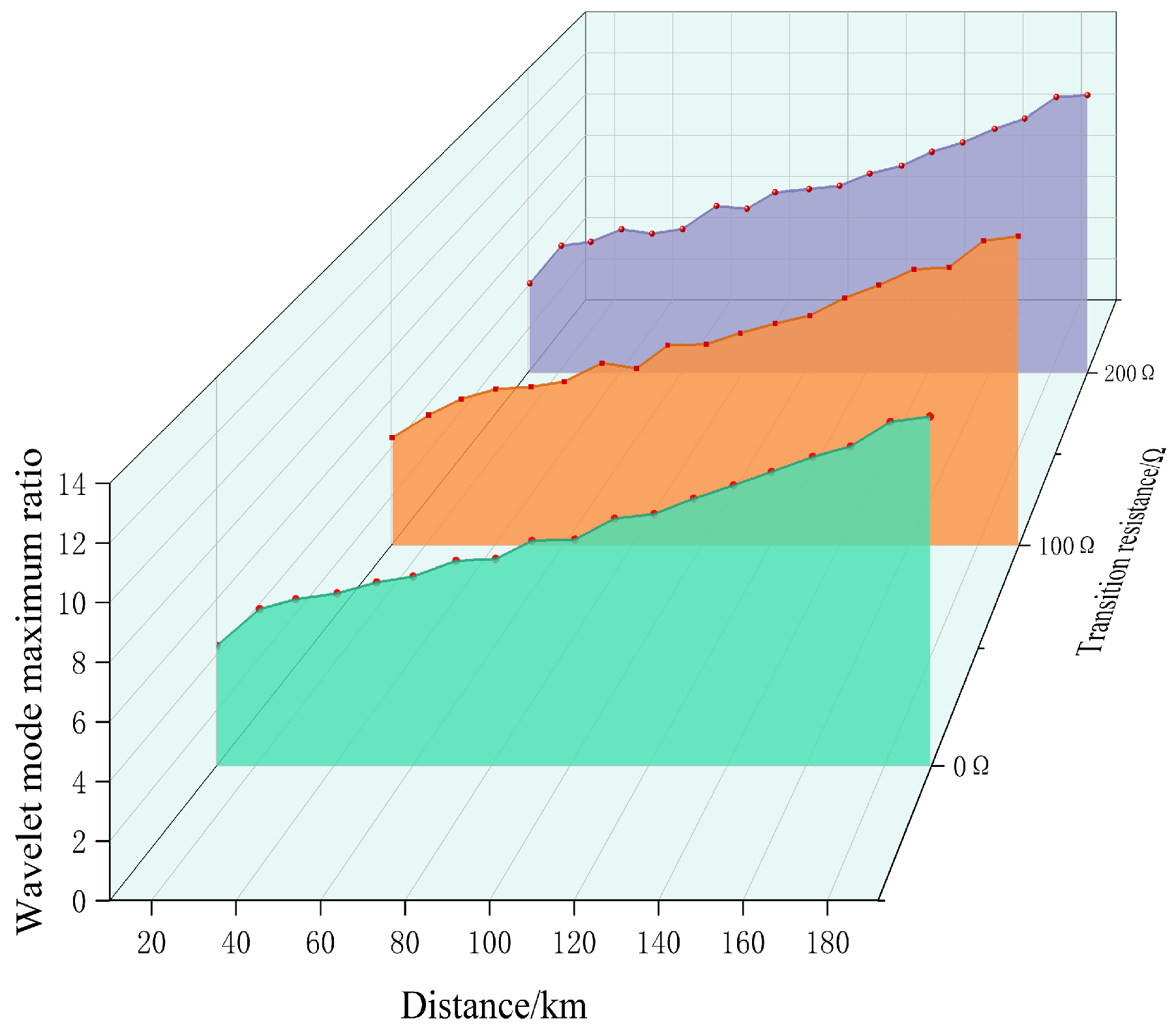
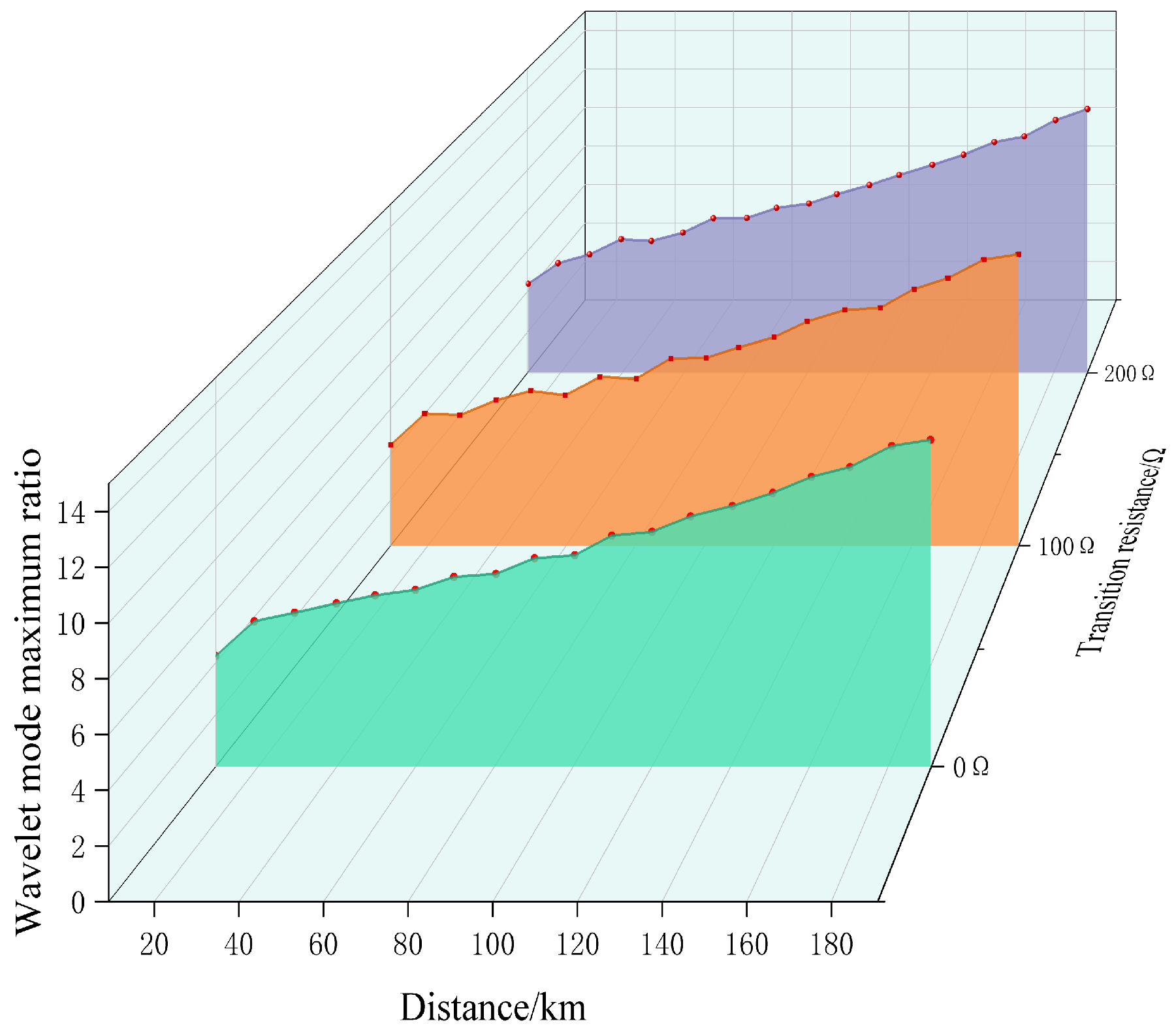
Under different transition resistance conditions, when an asymmetrical ground fault occurs, the d1-scale wavelet mode magnitude ratio between the sum of the 1-mode and 2-mode voltage components and the 0-mode component vary with the fault distance, as shown in Figure 4 and Figure 5.

From the figure, it can be seen that when a single-phase ground and two-phase ground fault occurs, the d1-scale wavelet mode magnitude ratio between the sum of the voltage 1-mode and 2-mode components and the 0-mode component is positively correlated with the distance from the fault in a nonlinear mapping.

3.2. Effect of Fault Initial Phase Angle on Ranging Effectiveness

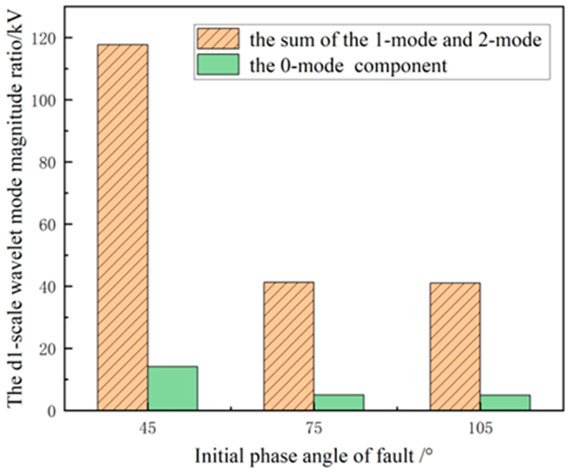
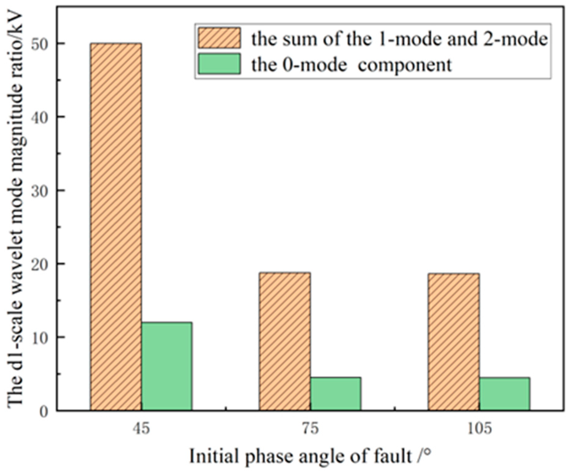
From the above analysis, it can be seen that the amplitude ratio of the sum of the 1-mode and 2-mode components and the 0-mode component of the voltage at the ranging place is independent of the initial phase angle of the fault [20]. In order to verify this inference, the measured initial transient voltage travelling wave is subjected to wavelet transform, and the wavelet mode maxima of the sum of the 1-mode and 2-mode components and the wavelet mode maxima of the 0-mode component of the initial transient voltage travelling wave at the d1 scale are obtained, as shown in Figure 6 and Figure 7.

From the figure, it can be seen that in the asymmetrical ground fault, the wavelet mode magnitude of the sum of the 1-mode and 2-mode components and the 0-mode component at the ranging device change with the change in the initial phase angle of the fault, and both wavelet mode magnitude ratios are unchanged, so the wavelet mode magnitude ratios of the sum of the 1-mode and 2-mode components and the 0-mode component of the travelling wave of the initial transient voltage have nothing to do with the initial phase angle of the fault, and the corresponding wavelet mode magnitude ratios are shown in

Table 4. The maximum ratio of single-phase grounding voltage d1-scale wavelet mode at different initial fault phase angles at 100 km from the fault.

Initial Phase Angle of the Fault/(°)	The d1-Scale Wavelet Mode Maximum		The Wavelet Mode Maximum Ratio
	The Sum of the 1-Mode and 2-Mode Voltage Components	The 0-Mode Voltage Component
45	117.76	14.12	8.34
75	41.28	4.95	8.34
105	41.03	4.92	8.34

and

Table 5. The maximum ratio of two-phase grounding voltage d1-scale wavelet mode at different initial fault phase angles at 100 km from the fault.

Initial Phase Angle of the Fault/(°)	The d1-Scale Wavelet Mode Maximum		The Wavelet Mode Maximum Ratio
	The Sum of the 1-Mode and 2-Mode Voltage Components	The 0-Mode Voltage Component
5	49.96	12.01	4.16
75	18.76	4.51	4.16
105	18.64	4.48	4.16

.

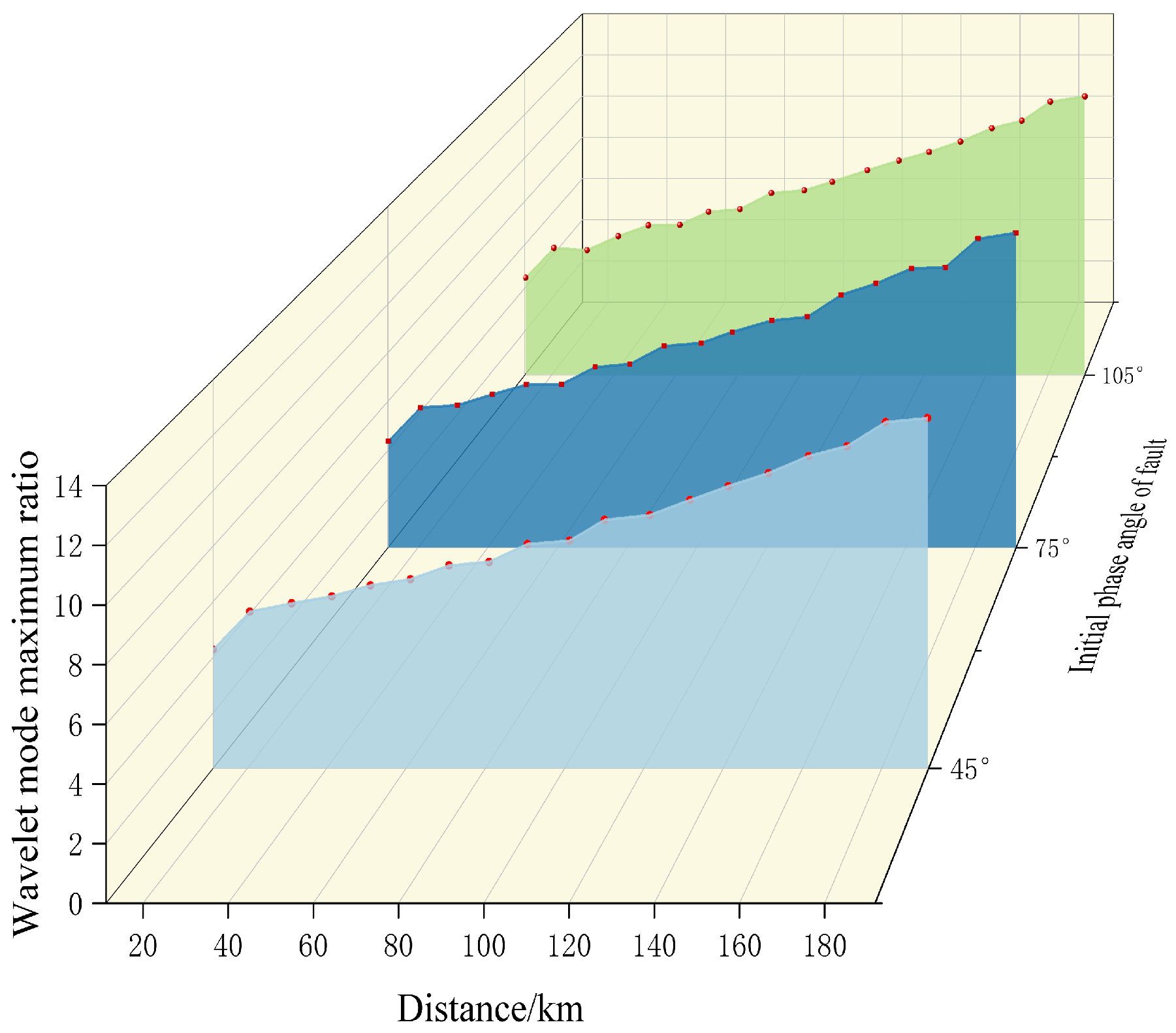
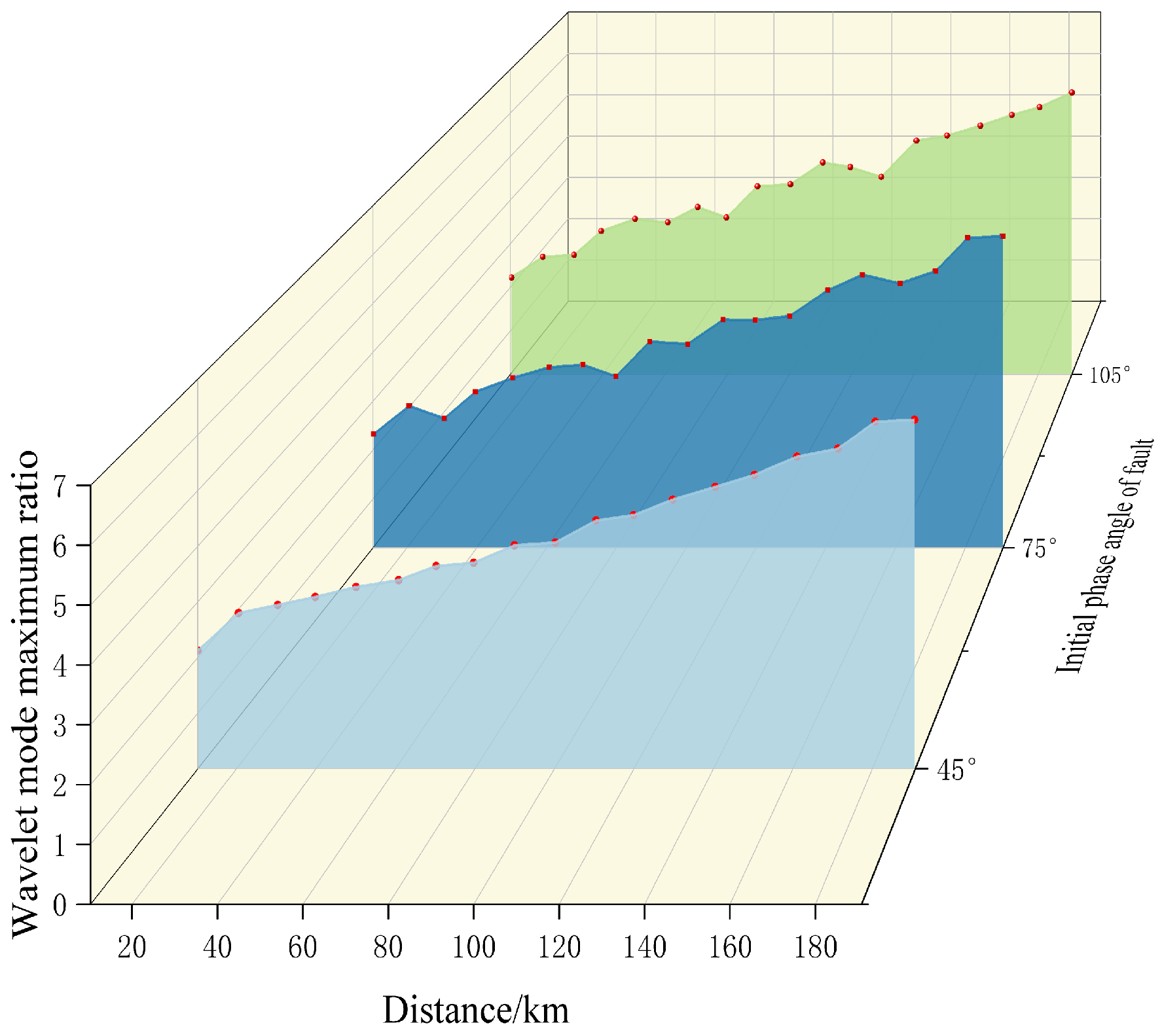
Under different fault initial phase angle conditions, when an asymmetrical ground fault occurs, the d1-scale wavelet mode magnitude ratio between the sum of the voltage mode 1 and 2 components and the mode 0 component varies with the fault distance, as shown in Figure 8 and Figure 9.

From the figure, it can be seen that the wavelet mode magnitude ratio between the sum of the initial transient voltage travelling wave 1-mode and 2-mode components and the 0-mode component is positively correlated with the fault distance by a nonlinear mapping.

4. Results

4.1. Attention-GRU Ranging Algorithms

4.1.1. The GRU Model

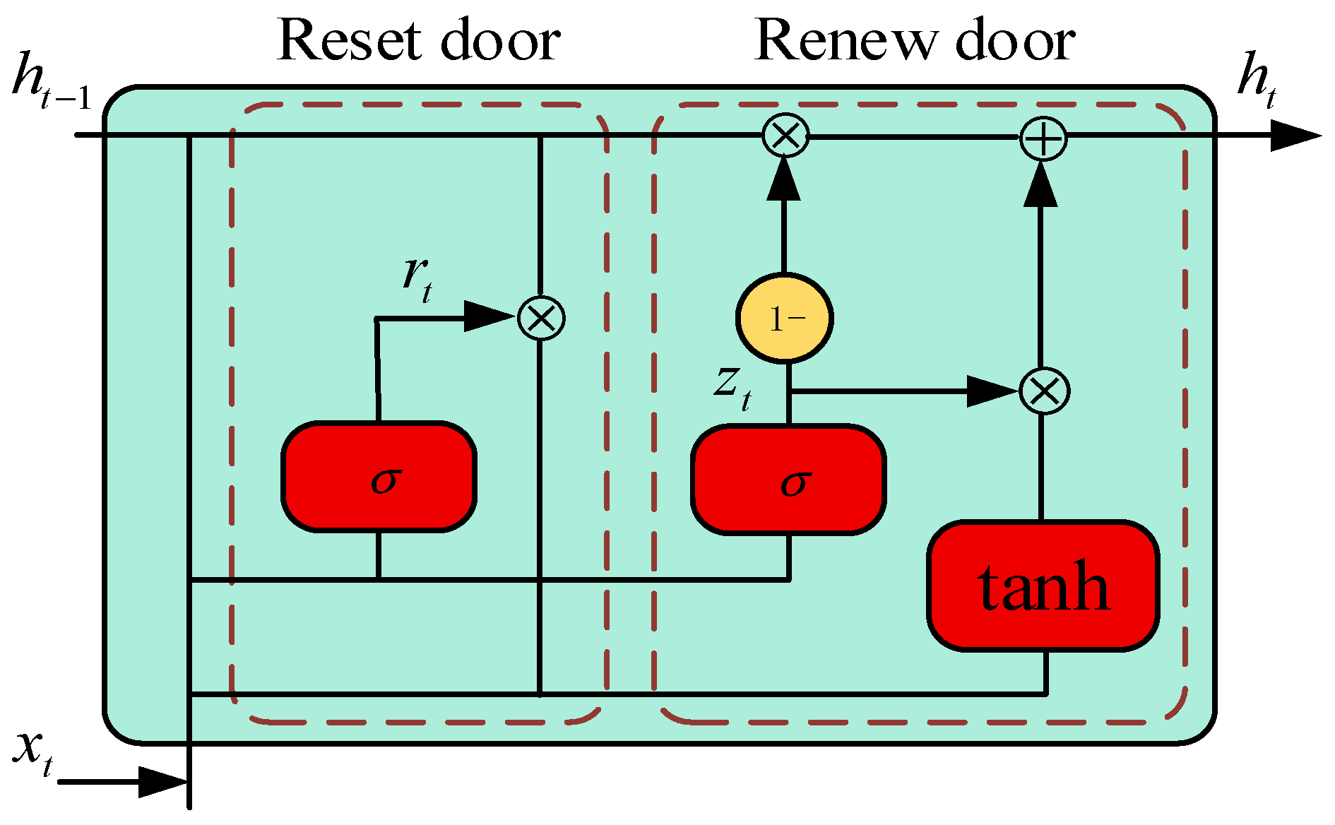
GRU (Gated Recurrent Unit) is a variant of RNN (Recurrent Neural Network) that is designed to solve the problems of gradient vanishing and gradient explosion that traditional RNNs face when dealing with long time-series data [21]. By introducing the update and reset gate mechanisms, GRU automatically determines the information that needs to be kept or forgotten at each time step, enabling it to better capture long-term dependencies in the data. Figure 10 shows the structure of the constructed GRU model.

The core structure of GRU consists of these two gates. Assuming the input data is $x_t$ and the hidden state at the previous moment is $h_{t-1}$, the GRU computation process includes the following steps [22]:

(1) In a reset gate, the relationship between the inputs of the current moment and the hidden state of the previous moment is controlled to determine whether the memory of the previous moment is retained:

$$r_t=\sigma \left(W_r\left[h_{t-1},x_t\right]+b_r\right)$$

(22)

where $r_t$ is the reset gate; $\sigma$ is the activation function; $W_r$ is the weight matrix; and $b_r$ is the bias term.

(2) For the update gate, the decision on how the information at the current moment is updated to the hidden state consists of two parts, i.e., the combination of the current input and the hidden state of the previous moment:

$$z_t=\sigma \left(W_z\left[h_{t-1},x_t\right]+b_z\right)$$

(23)

where $z_t$ is the update gate that determines how much of the current hidden state is partially from the previous moment’s hidden state.

(3) For candidate hidden states, the candidate hidden state at the current moment is computed. This value combines the input information of the current moment with the memorised information of the previous moment:

$$\stackrel{\sim }{h_t}=\tanh \left(W_h\left[r_t{h}_{t-1},x_t\right]+b_h\right)$$

(24)

(4) The final hidden state is based on the update gate $z_t$ and the candidate hidden state $\stackrel{\sim }{h_t}$:

$$h_t=\left(1-z_t\right)h_{t-1}+z_t\stackrel{\sim }{h_t}$$

(25)

The GRU can efficiently process long time series data by selectively and flexibly memorising important information while forgetting unimportant information at each time step through these gate mechanisms.

4.1.2. Attention Mechanism

Attention mechanism is an important technique in the field of deep learning, especially suitable for processing long time-series data. The core idea is to allow the model to dynamically assign different weights to different parts of the input so as to focus on the information that is most critical to the task [23]. The basic computational process of the attention mechanism consists of the following steps:

(1) Calculate the attention score. Based on the current hidden state $h_t$ and all historical hidden states $h_0,h_1,h_2,\dots ,h_{t-1}$, the attention score is computed for each moment. A common way to compute the attention score is by a weighted sum using a learnable parameter vector $v$:

$$\begin{array}{l}{e}_t=\mathrm{score}\left(h_t,h_1,h_2,\dots ,h_{t-1}\right)\\ ={\mathit{v}}^{\mathrm{T}}\tanh (w_{\mathrm{e}}{h}_{\mathrm{t}}+b_{\mathrm{e}})\end{array}$$

(26)

where $e_t$ is the attention score at the current moment; $w_e$ and $b_e$ are learnable parameters.

(2) Calculate the attention weights. A softmax operation is performed on the scores of all moments to obtain the attentional weight of each moment, indicating the importance of the information at that moment:

$${\alpha }_t={\displaystyle \frac{\exp (e_t)}{{\displaystyle {\sum }_{i=1}^t\exp (e_i)}}}$$

(27)

where ${\alpha }_t$ is the attention weight at moment $t$, representing the importance of the current moment relative to other moments.

(3) Calculate the weighted sum. Weight all hidden states according to the attention weights to obtain the weighted sum $c_t$, as the contextual information of the current moment:

$$c_t={\displaystyle \sum _{i=1}^t{\alpha }_i{h}_i}$$

(28)

(4) Output results. The final output is generated by combining the weighted sum $c_t$ and the hidden state.

$$y_t=\mathrm{output}(c_t,h_t)$$

(29)

The core advantage of introducing the attention mechanism into the GRU model for AC line fault ranging lies in its ability to dynamically assign different weights to the input features, so that the model intelligently focuses on the information points that are most critical for fault distance judgement, and effectively filters out the influence of noise or irrelevant features. This not only improves the model’s ability to capture complex nonlinear relationships and potential long-distance dependencies, and enhances the effectiveness of feature representation, but also provides interpretability for model decision-making through the visualisation of attention weights, which ultimately significantly improves the accuracy and reliability of fault ranging.

4.1.3. Attention-GRU Ranging Model Flowchart

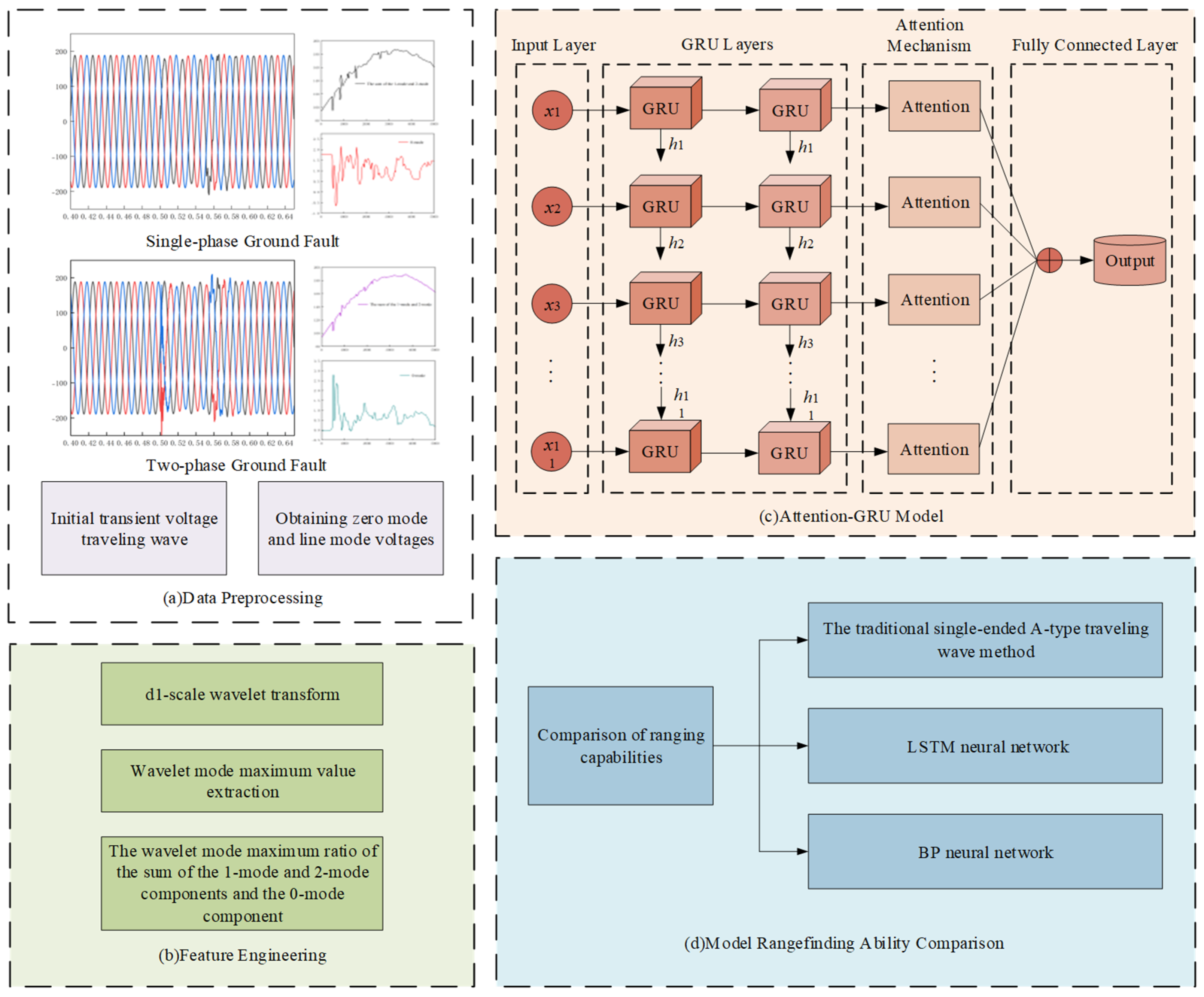
To enhance the accuracy of fault location in high-voltage AC transmission lines, this paper proposes an Attention-GRU fault location model, whose workflow is illustrated in Figure 11.

(1) Collect the initial transient voltage travelling wave signal at the ranging device and use the Karrenberg phase transformation to convert it into the corresponding magnitude travelling wave voltage signal.

(2) Create an Attention-GRU neural network ranging model and use a two-layer GRU network to extract time series features and introduce an attention mechanism. During training, use the Adam W optimiser combined with cosine annealing learning rate scheduling and output the prediction results through the fully connected layer.

(3) Use the ratio of the sum of the 1-mode and 2-mode voltage components to the maximum of the 0-mode wavelet component as the input feature vector [x₁, x₂, x₃, x₄, x₅, x₆, x₇, x₈, x₉, x₁₀, x₁₁], with the output vector being the fault distance. The dataset is divided into training and testing datasets. The training dataset is fed into the Attention-GRU distance estimation model for training.

(4) Apply the trained Attention-GRU distance estimation model to predict the test dataset and compare its distance estimation capabilities with those of traditional single-ended A-type travelling wave methods, LSTMs and BP neural network models.

4.2. Simulation and Result

The 220 kV high-voltage AC transmission line model is built on the PSCAD/EMTDC simulation platform, as shown in Figure 1. To ensure the generalisation capability of the neural network model, the sample data is divided into training, test, and validation sets. The training set comprises 80% of the samples, the test set comprises 10%, and the validation set comprises 10%.

In the simulation model, the fault type is set as single-phase ground fault, two-phase ground fault. The step size for fault point changes is 0.5 km, take the value range of 0~200 km; the transition resistance change step is $10 \mathrm{\Omega }$, take the value range of $0\sim 200 \mathrm{\Omega }$; the initial phase angle of the fault change step is $15°$, set the range of $-60°\sim 300°$. The generation method for training or test samples is random, with a seed value of 42.

4.2.1. Attention-GRU Neural Network Training

The Attention-GRU neural network model is constructed on the Python 3.10.12 platform and uses a two-layer GRU network to extract temporal features. It also introduces an attention mechanism containing two linear layers and a Tanh activation function to dynamically weight the hidden states of the GRU output, thereby enhancing the representation of key features. Finally, it outputs the prediction results through the fully connected layer. During training, the Adam W optimiser is used in conjunction with cosine annealing learning rate scheduling [24]. The loss function is mean square error (MSE), and an early stopping mechanism is employed to prevent overfitting. The final result is a fault ranging model with optimal generalisation ability [25]. The parameter settings of the Attention-GRU model are shown in

Table 6. Attention-GRU model parameter settings.

Parameter Name	Parameter Setting
Number of neurons in the input layer	11
Number of GRU units in the first layer	128
Number of GRU units in the second tier	128
Number of neurons in the Dense layer	1
First linear layer	16,512
Second linear layer	129
Hidden layer activation function	Tanh
Initial learning rate	0.001
Maximum number of iterations	150
Optimisation algorithm	Adam W

.

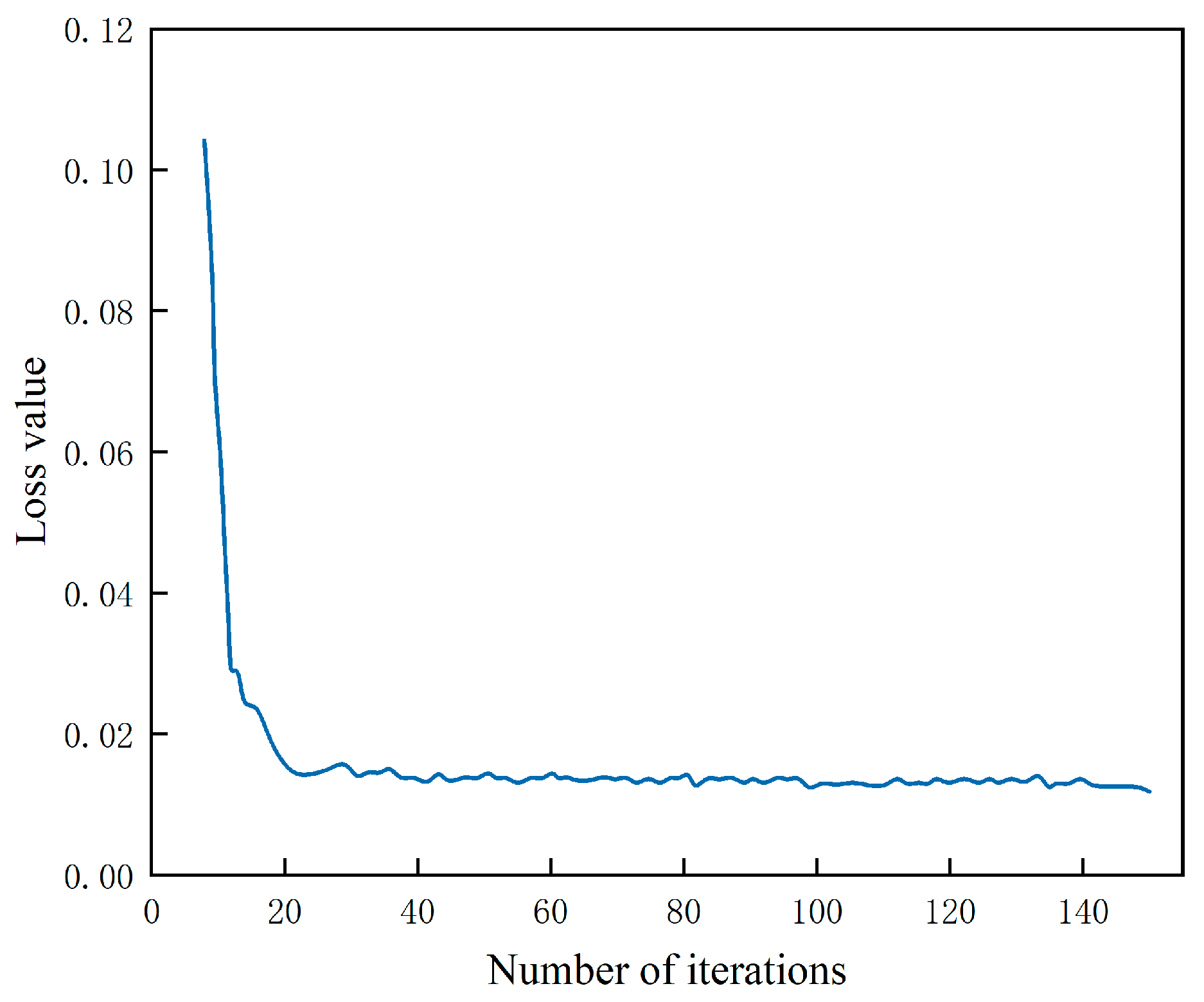
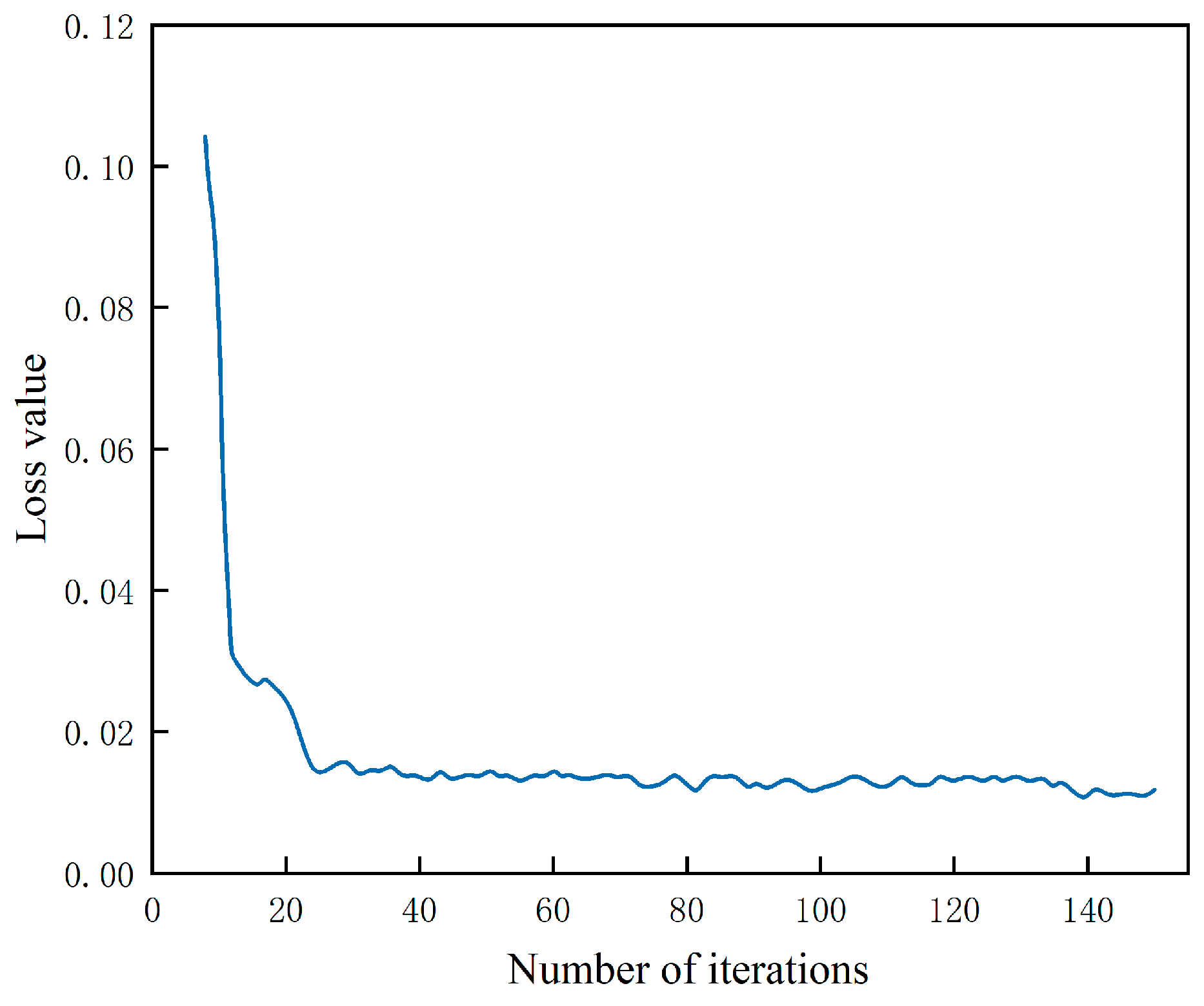
After completing the parameter configuration of the Attention-GRU model, the model is trained and optimised using training set samples. The training set loss curves for single-phase ground faults and two-phase ground faults are shown in Figure 12 and Figure 13, respectively.

As can be seen from the figure, the Attention-GRU neural network model achieves a loss value of 0.0099 for the training samples after 150 iterations, demonstrating fast convergence and high prediction accuracy.

4.2.2. Comparison of Ranging Capabilities Between Attention-GRU Model and Conventional Single-Ended A-Type Travelling Wave Method

Based on the line parameters in Table 1, the approximate estimated travelling wave velocity of the line model is $v_1\approx 1/\sqrt{LC}=2.93145\times {10}^5 \mathrm{km}$. Using the traditional single-ended A-type travelling wave method, the arrival times of the initial voltage travelling wave front and the second reflected wave front must be measured in order to calculate the distance [26]. The second reflected wave front can be identified by comparing the polarity of the reflected wave front at the fault point with that of the reflected wave front at the opposite busbar. The fault distance can then be calculated using the A-type travelling wave method distance calculation formula. The results of their range comparison are shown in

Table 7. Comparison of ranging results between the Attention-GRU model and the traditional single-ended A-type travelling wave method.

AG					BCG					Type A Travelling Wave Method Ranging Value/km	Absolute Error/km
Fault Distance/km	Initial Fault Phase Angles/(°)	Transition Resistance/Ω	Attention-GRU Ranging Value/km	Absolute Error/km	Fault Distance/km	Initial Fault Phase Angles/(°)	Transition Resistance/Ω	Attention-GRU Ranging Value/km	Absolute Error/km
30	45	120	30.29	0.29	30	45	120	29.74	0.26	29.47	0.53
75	45	120	75.14	0.14	75	45	120	75.21	0.21	75.33	0.33
125	45	120	124.88	0.12	125	45	120	124.95	0.05	126.21	1.21
65	35	100	65.42	0.42	65	35	100	64.72	0.28	66.72	1.72
65	75	100	65.31	0.31	65	75	100	65.38	0.38	64.12	0.88
65	115	100	65.54	0.54	65	115	100	64.66	0.34	66.45	1.45
150	60	160	150.52	0.52	150	60	160	149.76	0.24	151.58	1.58
175	75	160	175.66	0.66	175	75	160	175.49	0.49	175.98	0.98

.

Compared to the traditional A-type travelling wave method, the method proposed in this paper has significant advantages. It only requires the initial transient voltage travelling wave front to be collected and does not require the nature of the second reflected wave front to be identified, thereby improving ranging accuracy. Through experimental verification under different fault types, fault distances, initial fault angles and transition resistance conditions, the ranging error of the ranging model based on the Attention-GRU neural network for the test set samples was always kept within 1 km. This indicates that the method can accurately calculate fault distances and that its ranging performance is unaffected by factors such as fault type, location, transition resistance and initial phase angle, demonstrating greater robustness and reliability.

4.2.3. Comparison of Attention-GRU Neural Network with Other Neural Networks in Terms of Ranging Ability

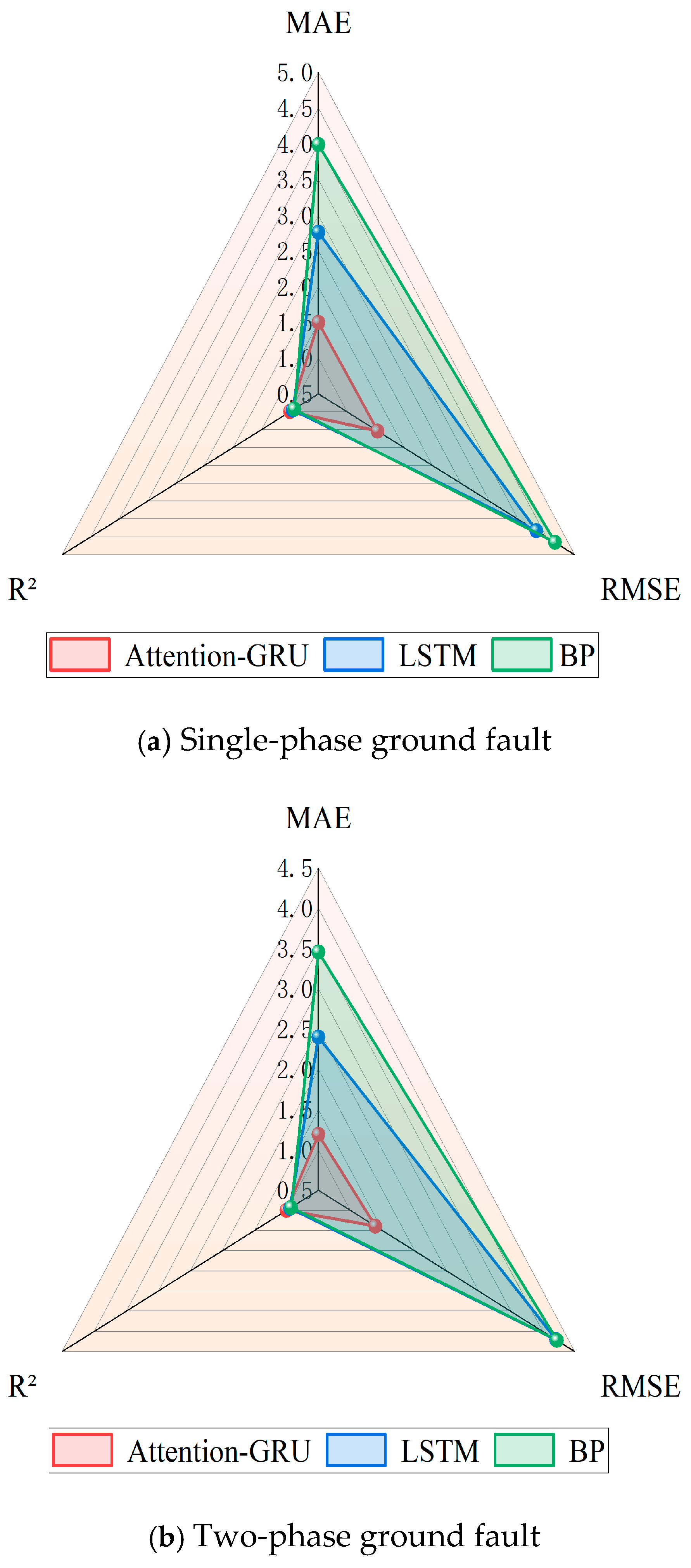
Once the Attention-GRU model has been trained, it can be used for fault ranging in cases of asymmetric grounding faults in high-voltage AC transmission lines. To systematically evaluate the performance of the Attention-GRU neural network in fault ranging, this paper selects the Long Short-Term Memory (LSTM) network and the back propagation (BP) neural network as comparison models [27]. The corresponding ranging models are constructed and compared, and the ranging results are shown in

Table 8. Comparison of fault ranging results between Attention-GRU model and other neural network models.

Fault Type	Fault Distance/km	Initial Fault Phase Angles/(°)	Transition Resistance/Ω	Attention-GRU Neural Network		LSTM Neural Network		BP Neural Network
				Ranging Value/km	Absolute Error/km	Ranging Value/km	Absolute Error/km	Ranging Value/km	Absolute Error/km
AG	20	30	0	20.30	0.30	21.28	1.28	22.17	2.17
	45	45	20	45.01	0.01	47.03	2.03	46.53	1.53
	66	60	40	66.26	0.26	67.46	1.46	67.81	1.81
	80	75	80	80.30	0.30	80.68	0.68	81.54	1.54
	88	95	100	88.87	0.87	89.69	1.69	89.95	1.95
	110	105	60	110.01	0.01	111.81	1.81	112.81	2.81
	130	75	120	130.40	0.40	132.54	2.54	131.02	1.02
	150	120	140	150.73	0.73	151.01	1.01	151.10	1.10
	170	150	100	170.36	0.36	171.26	1.26	171.82	1.82
	190	135	160	190.55	0.55	191.58	1.58	192.22	2.22
BCG	30	30	0	30.43	0.43	30.10	0.10	31.37	1.37
	47	45	20	47.26	0.26	48.27	1.27	48.12	1.12
	60	60	60	60.06	0.06	61.37	1.37	62.70	2.70
	85	95	40	85.28	0.28	86.46	1.46	86.13	1.13
	100	75	80	100.17	0.17	101.29	1.29	101.35	1.35
	121	60	120	121.49	0.49	121.95	0.95	122.95	1.95
	145	125	100	145.48	0.48	147.36	2.36	145.86	0.86
	165	140	140	165.26	0.26	167.05	2.05	166.46	1.46
	177	130	80	177.06	0.06	178.88	1.88	178.57	1.57
	190	150	160	190.84	0.84	191.11	1.11	191.44	1.44

. The model evaluation indexes are MAE (mean absolute error), RMSE (root mean-square error) and R² (coefficient of determination). Their evaluation results are shown in Figure 14. The LSTM neural network model parameters are set as follows: the hidden layer has 128 neurons, there are 2 LSTM layers, and the dropout rate is 0.2. The BP neural network model parameters are set as follows: the hidden layer has 8 neurons, tansig is used as the activation function, and pureline is used as the output layer activation function.

Table 8 shows that the Attention-GRU neural network outperforms the LSTM and BP neural networks in terms of asymmetric ground fault ranging accuracy and robustness, effectively improving the accuracy and reliability of fault ranging. The experimental results show that, in the case of a single-phase ground fault, the MAE (mean absolute error), RMSE (root mean-square error) and R² (coefficient of determination) of the Attention-GRU ranging model are 2.5008, 1.539 and 0.9963, respectively. In the case of a two-phase ground fault, these values are 1.192, 1.390 and 0.999, respectively. From these evaluation indexes, it can be seen that the model has excellent predictive ability and stability and can accurately capture changes in fault distance.

4.2.4. The Effect of Different Types of Noise on Range Measurement Performance

In actual power systems, measurement noise and electromagnetic interference in secondary circuits inevitably superimpose on fault transient travelling wave signals [14]. To validate the robustness of the proposed method under non-ideal operating conditions, varying levels of Gaussian white noise were introduced into the initial transient voltage travelling wave characteristics collected. The distance measurement comparison results are shown in

Table 9. Comparison of fault location results at different noise levels.

Noise Level/dB	Fault Type	Fault Distance/km	Initial Fault Phase Angles/(°)	Transition Resistance/Ω	Attention-GRU Neural Network		LSTM Neural Network		BP Neural Network
					Ranging Value/km	Absolute Error/km	Ranging Value/km	Absolute Error/km	Ranging Value/km	Absolute Error/km
10 dB	AG	55	45	80	56.27	1.27	58.77	3.77	58.39	3.39
	BCG	95	60	100	96.28	1.28	98.12	3.12	98.27	3.27
20 dB	AG	75	45	120	74.18	0.82	77.24	2.24	77.56	2.56
	BCG	85	75	110	85.76	0.76	87.21	2.21	87.33	2.33
30 dB	AG	75	95	140	75.59	0.59	76.89	1.89	76.94	1.94
	BCG	45	105	130	45.37	0.37	46.35	1.35	46.48	1.48
40 dB	AG	120	65	160	120.36	0.36	120.96	0.96	121.06	1.06
	BCG	145	95	140	145.19	0.19	145.94	0.94	145.84	0.84

.

As shown in Table 9, across tests with varying signal-to-noise ratios, the proposed Attention-GRU model significantly outperforms the compared neural network models in both positioning accuracy and stability. Particularly under severe conditions with strong noise interference, the ranging errors of the LSTM and BP models exhibit significant fluctuations, leading to a noticeable decline in accuracy. In contrast, the proposed model demonstrates superior robustness and noise immunity, effectively suppressing feature distortion caused by noise. Experimental results confirm that this method not only effectively mitigates the impact of non-ideal operating environments on extracting the maximum ratio of travelling wave mode, but also maintains high ranging accuracy under various extreme conditions, showcasing excellent field applicability and robustness.

4.2.5. The Effect of Different Sampling Frequencies on Range Measurement Performance

To systematically evaluate the effectiveness of the proposed algorithm in practical engineering applications, comparative analyses were conducted at three sampling frequencies—1 MHz, 100 kHz and 50 kHz—under various combinations of distance, transition resistance and initial fault phase angle. The distance measurement comparison results are presented in

Table 10. Comparison of fault location results at different sampling frequencies.

Fault Type	Fault Distance/km	Initial Fault Phase Angles/(°)	Transition Resistance/Ω	1 MHz Sampling Frequency		100 kHz Sampling Frequency		50 kHz Sampling Frequency
				Ranging Value/km	Absolute Error/km	Ranging Value/km	Absolute Error/km	Ranging Value/km	Absolute Error/km
AG	65	35	30	65.15	0.15	65.62	0.62	66.25	1.25
AG	65	75	200	65.28	0.28	65.85	0.85	66.58	1.58
BCG	100	45	50	100.42	0.42	101.12	1.12	101.95	1.95
BCG	100	60	150	100.76	0.76	101.38	1.38	102.31	2.31
AG	150	55	30	150.68	0.68	151.55	1.55	152.14	2.14
AG	150	120	200	150.82	0.82	151.92	1.92	152.34	2.34

.

As shown in Table 10, ranging error increases as sampling frequency decreases from 1 MHz to 50 kHz (an industrial grade), due to the influence of quantisation sparsity at the sampling point. Experiments demonstrate that the modulus-to-amplitude ratio feature extracted in this paper reflects the overall attenuation mapping pattern of travelling wave propagation. This feature exhibits significantly lower dependence on sampling frequency than the time calibration features of traditional travelling wave methods. Even under low-frequency sampling conditions, the algorithm demonstrates exceptional tolerance to transition resistances and provides robust initial phase angle accuracy. These comparisons conclusively demonstrate that this algorithm achieves outstanding ranging stability without requiring ultra-high sampling rate hardware, thereby meeting the engineering application requirements for existing power system relay protection devices.

4.2.6. Analysis of Computational Efficiency and Real-Time Performance

To evaluate the real-time application performance of the proposed ranging model in engineering practice, this paper conducts a comparative analysis of the computational costs for the Attention-GRU, LSTM and BP neural network models. The convergence iterations, offline training time and online inference efficiency for each model are shown in

Table 11. Comparative analysis of computational efficiency among different neural network models.

Types of Neural Networks	Convergence Iteration Count	Total Offline Training Time (s)	Average Inference Time per Sample (ms)
Attention-GRU	150	145.2	1.32
LSTM	180	198.5	1.86
BP	220	12.4	1.86

.

As shown in Table 11, the Attention-GRU model has a significantly faster offline training speed and more efficient inference than the LSTM model. With an average inference time of just 1.32 ms, it fully meets the stringent real-time requirements for fault location in power systems. The proposed method strikes an optimal balance between computational cost and location accuracy. Furthermore, its low parameter count and feature dimension make it highly feasible for engineering deployment.

5. Conclusions

This paper proposes a high-voltage AC transmission line asymmetric grounding fault ranging method based on deep learning and modulus amplitude ratio, aiming to address the issues associated with travelling wave ranging methods in asymmetric grounding faults of high-voltage AC transmission lines. This method offers high computational efficiency, robustness and generalisation ability. Through theoretical analysis and simulation verification, the following conclusions were obtained:

(1) The fault distance exhibits a deterministic, nonlinear mapping relationship with the ratio of the amplitude of the sum of the first and second mode components of the initial transient voltage travelling wave at the measurement point, divided by the zero mode component. This relationship is independent of the transition resistance and the initial phase angle of the fault, which effectively reduces the impact of external interference factors on the distance measurement results.

(2) This method only requires the initial transient voltage travelling wavefront signal to be acquired at the distance measurement device, successfully resolving the challenge of identifying reflected wavefronts in single-ended travelling wave distance measurement.

(3) Extracting the amplitude of the initial transient voltage travelling wave front effectively avoids inaccuracies in wavefront arrival time calibration caused by travelling wave dispersion characteristics.

(4) Simulation verification demonstrates that the proposed distance measurement model significantly outperforms Type A travelling wave, LSTM and BP neural network distance measurement models in terms of accuracy. Furthermore, its distance measurement capability remains largely unaffected by the type of fault, transition resistance and initial fault phase angle.

References

1. Lu, D.; Liu, Y. Fault location for general AC/DC transmission lines: Multi-phase, non-homogeneous, partially mutually coupled and multi-terminal lines. Electr. Power Syst. Res. 2023, 222, 109484. [Google Scholar] [CrossRef] [Scilit]
2. Wan, W.; Qin, Z.; Deng, M.; Liu, Y. Traveling wave network location method based on adaptive waveform similarity. Heliyon 2024, 10, e37576. [Google Scholar] [CrossRef] [Scilit]
3. Zeng, J.; Zeng, X.; Bai, H.; Yu, K.; Xu, M.; She, X.; Liu, F. A novel fault location method for multi-terminal transmission lines based on composite analysis of time-frequency fault traveling waves. Int. J. Electr. Power Energy Syst. 2025, 167, 110600. [Google Scholar] [CrossRef] [Scilit]
4. Liu, F.; Xie, L.; Yu, K.; Wang, Y.; Zeng, X.; Bi, L.; Tang, X. A novel fault location method based on traveling wave for multi-branch distribution network. Electr. Power Syst. Res. 2023, 224, 109753. [Google Scholar] [CrossRef] [Scilit]
5. Xie, L.; Luo, L.; Ma, J.; Li, Y.; Zhang, M.; Zeng, X.; Cao, Y. A novel fault location method for hybrid lines based on traveling wave. Int. J. Electr. Power Energy Syst. 2022, 141, 108102. [Google Scholar] [CrossRef] [Scilit]
6. Yu, K.; Zhu, X.; Cao, W. Study on traveling wave fault localization of transmission line based on NGO-VMD algorithm. Energies 2024, 17, 2003. [Google Scholar] [CrossRef] [Scilit]
7. Huai, Q.; Liu, K.; Hooshyar, A.; Ding, H.; Chen, K.; Liang, Q. Single-ended line fault location method for multi-terminal HVDC system based on optimized variational mode decomposition. Electr. Power Syst. Res. 2021, 194, 107054. [Google Scholar] [CrossRef] [Scilit]
8. Wang, Y.; Xie, L.; Liu, F.; Yu, K.; Zeng, X.; Bi, L.; Tang, X. Fault location method for distribution network Considering distortion of traveling wavefronts. Int. J. Electr. Power Energy Syst. 2024, 159, 110065. [Google Scholar] [CrossRef] [Scilit]
9. Qiu, L.; Ai, Y.; Liu, J.; Xie, C.; Fu, H.; Yan, Y. Fault location technology for cable-overhead-hybrid transmission lines based on improved HOVMD-TKEO and wave velocity normalization method. IEICE Electron. Express 2024, 21, 20240431. [Google Scholar] [CrossRef] [Scilit]
10. Ye, X.; Lan, S.; Xiao, S.J.; Yuan, Y. Single Pole-to-Ground Fault Location Method for MMC-HVDC System Using Wavelet Decomposition and DBN. IEEJ Trans. Electr. Electron. Eng. 2021, 16, 238–247. [Google Scholar] [CrossRef] [Scilit]
11. Ye, Q.; Chen, T.; Zhong, Z.; Li, Z.; Zhang, Q. Transmission Line Fault Diagnosis Based on CNN-GRU Neural Network. In Proceedings of the 2022 15th International Symposium on Computational Intelligence and Design (ISCID), Hangzhou, China, 17–18 December 2022; IEEE: New York City, NY, USA, 2022; pp. 57–61. [Google Scholar]
12. Jia, T.; Yao, L.; Yang, G. A new fault location method for high-voltage transmission lines based on ICEEMDAN-MSA-ConvGRU model. IET Gener. Transm. Distrib. 2024, 18, 2650–2668. [Google Scholar] [CrossRef] [Scilit]
13. Yu, Y.; Si, X.; Hu, C.; Zhang, J. A review of recurrent neural networks: LSTM cells and network architectures. Neural Comput. 2019, 31, 1235–1270. [Google Scholar] [CrossRef] [Scilit] [PubMed]
14. Ding, S.; Su, C.; Yu, J. An optimizing BP neural network algorithm based on genetic algorithm. Artif. Intell. Rev. 2011, 36, 153–162. [Google Scholar] [CrossRef] [Scilit]
15. Liang, R.; Liu, C.; Peng, N.; Cheng, M.; Wang, F. Fault location for power grid based on transient travelling wave data fusion via asynchronous voltage measurements. Int. J. Electr. Power Energy Syst. 2017, 93, 426–439. [Google Scholar] [CrossRef] [Scilit]
16. Wang, W.; Gao, X.; Fan, B.; Zeng, X.; Yao, G. Faulty phase detection method under single-line-to-ground fault considering distributed parameters asymmetry and line impedance in distribution networks. IEEE Trans. Power Deliv. 2021, 37, 1513–1522. [Google Scholar] [CrossRef] [Scilit]
17. Dong, X.; Shi, S. Identifying single-phase-to-ground fault feeder in neutral noneffectively grounded distribution system using wavelet transform. IEEE Trans. Power Deliv. 2008, 23, 1829–1837. [Google Scholar] [CrossRef] [Scilit]
18. Wang, L.; Liu, H.; Dai, L.V.; Liu, Y. Novel method for identifying fault location of mixed lines. Energies 2018, 11, 1529. [Google Scholar] [CrossRef] [Scilit]
19. Li, B.; Shi, L.; Wen, W.; Li, B.; Chen, X.; Su, J. Research on a New Single-End Fault Location Method for Single-Phase Grounding Faults of Transmission Lines Through Transition Resistance. Front. Energy Res. 2021, 9, 772345. [Google Scholar] [CrossRef] [Scilit]
20. Mirzaei, M.; Ab Kadir, M.Z.A.; Moazami, E.; Hizam, H. Review of fault location methods for distribution power system. Aust. J. Basic Appl. Sci. 2009, 3, 2670–2676. [Google Scholar]
21. Shewalkar, A. Performance evaluation of deep neural networks applied to speech recognition: RNN, LSTM and GRU. J. Artif. Intell. Soft Comput. Res. 2019, 9, 235–245. [Google Scholar] [CrossRef] [Scilit]
22. Kumar, B.R.; Mohapatra, A.; Chakrabarti, S.; Kumar, A. Phase angle-based fault detection and classification for protection of transmission lines. Int. J. Electr. Power Energy Syst. 2021, 133, 107258. [Google Scholar] [CrossRef] [Scilit]
23. Lynn, H.M.; Pan, S.B.; Kim, P. A deep bidirectional GRU network model for biometric electrocardiogram classification based on recurrent neural networks. IEEE Access 2019, 7, 145395–145405. [Google Scholar] [CrossRef] [Scilit]
24. Niu, Z.; Zhong, G.; Yu, H. A review on the attention mechanism of deep learning. Neurocomputing 2021, 452, 48–62. [Google Scholar] [CrossRef] [Scilit]
25. Bon, N.N. Deep Learning Method for Fault Diagnosis in High Voltage Transmission Lines: A Case of the Vietnam 220 kV Transmission Line. Int. J. Electr. Eng. Inform. 2022, 14, 254–275. [Google Scholar]
26. Yu, Y.; Liu, L.; Zhou, Z.; Du, Z.; Jiao, C. Identification method for pulse wave resulted from fault transient of overhead transmission line. IEEE Access 2023, 11, 32006–32017. [Google Scholar] [CrossRef] [Scilit]
27. Zhao, H.; Sun, S.; Jin, B. Sequential fault diagnosis based on LSTM neural network. IEEE Access 2018, 6, 12929–12939. [Google Scholar] [CrossRef] [Scilit]
Figure 1. Topology of high-voltage AC transmission line.
Energies 19 00494 g001
Figure 2. The maximum value of the wavelet mode of the single-phase ground voltage d1-scale is determined at 100 km from the fault via different transition resistances.
Energies 19 00494 g002
Figure 3. The maximum value of the wavelet mode of the two-phase ground voltage d1-scale is determined at 100 km from the fault via different transition resistances.
Energies 19 00494 g003
Figure 4. Plot of voltage d1-scale wavelet mode magnitude ratio with fault distance for single-phase grounding with different transition resistances.
Energies 19 00494 g004
Figure 5. Plot of voltage d1-scale wavelet mode magnitude ratio with fault distance for two-phase grounding with different transition resistances. Conclusions.
Energies 19 00494 g005
Figure 6. The maximum value of single-phase grounding voltage d1-scale wavelet mode at different initial fault phase angles at 100 km from the fault.
Energies 19 00494 g006
Figure 7. The maximum value of two-phase grounding voltage d1-scale wavelet mode at different initial fault phase angles at 100 km from the fault.
Energies 19 00494 g007
Figure 8. Plot of voltage d1-scale wavelet mode magnitude ratio at single-phase grounding with fault distance for different fault initial phase angles.
Energies 19 00494 g008
Figure 9. Plot of voltage d1-scale wavelet mode magnitude ratio at two-phase grounding with fault distance for different fault initial phase angles.
Energies 19 00494 g009
Figure 10. GRU model structure diagram.
Energies 19 00494 g010
Figure 11. Attention-GRU ranging model flowchart.
Energies 19 00494 g011
Figure 12. Training set loss value curves for single-phase ground faults.
Energies 19 00494 g012
Figure 13. Training set loss value curves for two-phase ground faults.
Energies 19 00494 g013
Figure 14. Chart of results for evaluation indicators.
Energies 19 00494 g014