Article

Residential Electrical Load, Solar Energy and Electricity Bill Forecasting Using Hybrid Machine Learning Models with Time-of-Use Tariffs: A Case Study of Durban, South Africa

by
Temitope Adefarati
1,
Gulshan Sharma
1,*,
Pitshou N. Bokoro
1 and
Rajesh Kumar
2,3
1
Department of Electrical & Electronic Engineering Technology, University of Johannesburg, Johannesburg 2094, South Africa
2
Department of Human Anatomy and Physiology, Faculty of Health Sciences, University of Johannesburg, Johannesburg 2094, South Africa
3
Department of Electrical Engineering, Malaviya National Institute of Technology, Jaipur 302017, India
*
Author to whom correspondence should be addressed.
Energies 2026, 19(18), 4414; https://doi.org/10.3390/en19184414 (registering DOI)
Submission received: 4 June 2026 / Revised: 20 July 2026 / Accepted: 21 July 2026 / Published: 18 September 2026

Abstract

Accurate forecasting of energy consumption, renewable power output and utility expenditure is essential for sustainable planning of residential buildings and improving smart grid integration. This study presents several techniques such as random forest, gradient boosting regression, extreme gradient boosting, deep belief networks, random vector functional link, multi-layer perceptron and hybrid ensemble for forecasting of residential load demand, electricity bills, solar energy generation and solar irradiance. Electricity bills under Time-of-Use tariffs are introduced in the paper to accomplish realistic evaluation of economic implications and facilitation of optimized energy usage and cost savings using real-time residential energy data collected from Durban, South Africa. The performance of the forecasting model is assessed by root mean square error (RMSE), mean absolute error (MAE), mean squared error (MSE), coefficient of determination (R2) and mean absolute scaled error (MASE). The outcomes of the study show that the hybrid ensemble model accomplished the highest forecasting accuracy of the electricity bill with MAE, RMSE, MSE, MASE and R2 of 0.018126, 0.022961, 0.00052719, 0.30006 and 0.97978 when compared to other models. The findings of the research can be used as potential benchmarks for intelligent tariff forecasting, demand response planning, smart energy management and renewable energy integration in residential buildings.

1. Introduction

The rapid growth in global electricity demand caused by population growth, industrial revolution, urbanization, digitalization, economic growth and high standard of living has led to an excessive reliance on the grid [1,2]. The energy consumption of the residential sector increased by 40–60% in developing countries over the past two decades despite electricity price mechanisms introduced globally through market reforms [3]. The integration of renewable energy sources (RESs) into residential buildings has changed many households from consumers to prosumers [4]. The proliferation of traditional power systems with smart metres, sensing technologies, automated control system and smart grid features has necessitated accurate forecasting of renewable energy generation, residential electrical load demands and electricity bills to improve grid sustainability, increase energy management and support technical and economic decisions of stakeholders of the power system [5,6]. The integration of renewable energy technologies into the residential buildings can cause variability and uncertainty of power supply due to the intermittent nature of weather conditions and change in seasonal climatic patterns [7]. The stochastic nature of solar resources has created a complicated challenge for the power system operators to accurately forecast household load demands and electricity bills under the dynamic tariff mechanism [8]. The Time-of-Use (TOU) electricity tariffs, based on the electricity pricing regimes such as peak, standard and off-peak periods, are used by utilities to regulate load demand and reduce grid congestion. TOU pricing mechanisms are introduced by electric utilities, energy regulators, system operators, policy makers, researchers and data analysists to improve demand side flexibility and promote home appliances shifting [9].
Forecasting techniques have undergone significant advancement in the past few decades by changing from traditional statistical techniques to sophisticated machine learning (ML) approaches [10]. The abovementioned techniques can be utilized in the power system for load forecasting, electricity price prediction, renewable energy generation prediction, energy management, operational planning and economic decision-making. Traditional statistical forecasting techniques are suitable for linear, stationary and well-structured time-series data. However, their performances are drastically affected by highly nonlinear, stochastic and multi-variable systems such as embedded renewable energy operation with smart grid, tariff mechanism, appliance usage patterns, consumer’s power consumption behaviour and weather variables [11]. These limitations can be addressed by using ML techniques that have proved to be more effective at modelling complicated time-dependent and nonlinear energy consumption behaviours of consumers. The application of single-model ML techniques in highly dynamic residential energy datasets can suffer from overfitting, instability and limited generalization capability due to limited or imbalanced data, behavioural uncertainty, renewable energy variability, poor temporal representation, excessive model complexity, poor hyperparameter tuning, lack of regularization and training and validation issues [12]. The shortcomings of using single model ML models for the prediction of residential building parameter can be addressed by hybridizing multiple ML models. Hybrid systems combined complementary techniques to increase prediction accuracy. This is achieved by using the strengths of each model while mitigating their intrinsic weaknesses [13]. Hybrid ML models can be used in the power system to integrate historical load data and meteorological parameters to forecast not only electrical demand and PV output but also real-time electricity bills [14]. The accuracy of electricity bill forecasting under TOU tariffs is crucial for households of developing countries whose incomes vary according to changes in energy prices [15]. Electricity bill prediction tools allow households to optimize the scheduling of appliances, increase self-consumption of solar energy, reduce peak-period usage and improve participation in demand response programmes [16].
Recent studies have been focused on the ML models to improve the robustness and accuracy of forecasting of the power systems due to their capability to model nonlinear relationships and process large-scale energy datasets. Li et al. [17] proposed a hybrid model for forecasting of load demands based on the combination of empirical mode decomposition and random forest (RF) approaches. The study showed that the decomposition-supported RF model considerably greatly increased forecasting accuracy and decreased prediction uncertainty under varying load demand circumstances. Mosetlhe and Yusuff [18] presented RF regression schemes to forecast energy demand of residential building. The results obtained from the study demonstrated that RF models reflected fluctuation of household energy usage trends and produced lower forecasting errors in comparison to traditional regression techniques. Parizad et al. [19] applied a hybrid ML approach for forecasting of residential energy demand and electricity price forecasting using a gradient boosting regression (GBR) algorithm. The results showed that boosting-based algorithms models performed better when predicting electricity costs under dynamic pricing conditions. Saini et al. [20] proposed a probabilistic GBR model integrated with iterative seasonal trend decomposition and multi-approach feature selection for short-term load forecasting. It can be seen from the outcomes of the research that the GBR models considerably increased the forecasting accuracy by capturing nonlinear and seasonal features of electricity load demand. Cui et al. [21] applied extreme gradient boosting (XGBoost) in a hybrid model for short-term electrical load prediction. It can be established from the outcomes of the study that XGBoost accomplished superior forecasting accuracy owing to its effective feature learning competence and robustness against overfitting. Yu et al. [22] presented the combination of Bayesian and XGBoost models in an error-weighted ensemble system for forecasting of household electricity load demand. It can be seen from the outcomes of the study that there is a significant reduction in RMSE and MAE values when compared to standalone ML models.
Han et al. [23] applied deep belief networks (DBN) model in forecasting the power output of photovoltaic based renewable energy systems. The findings of their study demonstrated that DBN models increased the prediction accuracy of solar power generation by learning hidden representations from historical solar generation data and meteorological variables. Similarly, Wu et al. [24] developed an improved DBN-based intelligent load identification and prediction model where DBN was optimized using a sparrow search algorithm. It can be established from the outputs of the study that DBN significantly improved feature extraction competence in nonlinear load data. This makes the model suitable for complex smart grid environments. In the same way, Shin et al. [25] presented a hybridization approach of hybrid variational mode decomposition and random vector functional link networks (RVFL) for short-term forecasting of load demand. The authors achieved high forecasting accuracy and lower computational complexity with proposed model when compared with the conventional deep learning approaches. Katuwal et al. [26] utilized a deep RVFL neural network for forecasting of nonlinear applications. The RVFL model is utilized in the study to improve generalization capability and reduce forecasting uncertainty of dynamic datasets. Peplinski et al. [27] proposed a ML approach for forecasting household electricity demand based on large-scale smart metre data integrated with weather, building and social and economic information. Zhou et al. [28] proposed smart metre data and probabilistic deep learning (DL) techniques for forecasting of residential electrical load demand. The findings of the research showed that multi-layer perceptron (MLP) models can effectively learn complicated consuming behaviours from historical data when preprocessing and feature representation are used correctly.
Banik and Biswas [29] incorporated RF and XGBoost models into a meta-learning architecture for forecasting of renewable energy and load demand. The authors utilized RF as a base learner to capture nonlinear correlations in input features and XGBoost was used in the study to increase prediction accuracy by correcting residual errors from the first stage model. The outcomes of the study show that hybridization of RF and XGBoost improved prediction accuracy and reduced error metrics when compared with standalone ML models that are utilized in forecasting of renewable energy applications. Cui et al. [21] applied a short-term load forecasting approach that combined XGBoost and RF features for accurate prediction of load demands. It can be seen from the outcomes of the study that the hybrid approach has considerably reduced forecasting accuracy, reduced error metrics and increased robustness under fluctuating load demands and weather conditions relative to conventional forecasting approaches. Muqtadir et al. [30] presented an ensemble of boosting ML models such as LightGBM, XGBoost and CatBoost for forecasting of residential electricity load demand. The work focused on short-term prediction by taking into account the nonlinear and intermittent nature of household energy usage in smart grid systems. The research results have shown that the proposed approach significantly improved forecasting accuracy by removing overfitting and capturing complicated temporal–spatial relations in load data. In addition, the authors also pointed out that the combination of multiple gradient boosting methods in a well-designed ensemble greatly enhanced prediction stability and robustness at various residential locations. Simaiya et al. [31] proposed hybrid model using transfer learning that combined XGBoost and LightGBM algorithms for energy forecasting in the smart grid. The research demonstrated that the proposed hybrid models significantly improved both computational performance and forecasting reliability.
Several critical research gaps have not been fully addressed in the literature despite significant progress in electricity demand forecasting and energy management using ML techniques. There are limited studies that simultaneously modelled residential electrical load, solar energy generation, solar irradiance and electricity bill forecasting within a unified hybrid ensemble technique under TOU pricing schemes. There is a limited number of studies that presented forecasting models by utilizing several geographical datasets and climatic conditions of developing nations. Most existing models are developed and tested using datasets from developed nations. The proposed datasets do not accurately reflect energy consumption trends in emerging economies. The significance portion of existing research is focused on electricity demand forecasting accuracy without considering the integration of forecasting models with practical energy management strategies. In addition, several forecasting models are developed using synthetic datasets that do not adequately represent real-time operating conditions of residential energy systems. Finally, limited attention has been given to the application of ML techniques in residential energy forecasting. The influence of different variables is essential for improving decision-making and policy development since the energy system has become data driven. Therefore, there is a clear need for ML techniques that integrate multiple predictive algorithms, incorporate RESs, utilize real-time datasets and support residential energy management strategies.
The abovementioned gaps are addressed in this study by proposing a hybrid ensemble forecasting framework that integrated multiple machine learning models to improve prediction accuracy and robustness. The performance of the proposed model is comprehensively evaluated using several statistical metrics and compared with state-of-the-art of forecasting models. This study presents forecasting techniques that consist of random forest, gradient boosting regression, XGBoost, deep belief networks, random vector functional link networks, multi-layer perceptron and hybrid ensemble. The hybridization of several models is utilized in the study to improve forecasting accuracy and maximize energy efficiency of the household system that is located in Durban, South Africa. The proposed models are used for residential electricity demand forecasting and energy management in response to residential buildings energy challenges of Durban. The study area is a metropolitan city that is characterized by humid climate, high solar irradiation and high residential load demand owing to population growth and urbanization. Multiple machine learning algorithms are presented in the paper to evaluate the forecasting accuracy and robustness of each model under dynamic operating conditions. The performance of the proposed models is assessed using real-time residential energy datasets and the comparative analysis based on the statistical metrics. This study provides several significant contributions to the field of residential energy forecasting and smart grid management. The major contributions of this research are presented as follows:
   i.
Development of forecasting approaches that integrated load demand, solar irradiance, renewable energy and electricity bill prediction using real-time data collected from Durban, South Africa.
  ii.
Comparative assessment of machine learning models such as RF, GBR, XGBoost, DBN, RVFL, MLP and hybrid ensemble techniques.
 iii.
Presentation of an ensemble hybrid model that utilized the complementary strengths of one model to overcome the weakness of another model.
 iv.
Assessment of forecasting performance by utilizing statistical metrics such as MAE, RMSE, MASE, MSE and R2.
  v.
Application of the proposed models in residential energy systems to establish their effectiveness and increase the forecasting accuracy.
 vi.
Integration of TOU tariff schemes into electricity bill forecasting for realistic economic evaluation and optimized residential energy management.
The remaining sections of the paper are organized as follows: Section 2 describes the materials and methods that consist of data collection, data preprocessing, machine learning model development and performance evaluation. Section 3 presents the results and discussion of the study that include forecasting accuracy, performance analysis of different techniques and comparative performance of the models. Finally, Section 4 concludes the paper with the key findings, contributions and future research prospects.

2. Materials and Methods

The research design is implemented in this study to provide a systematic system for developing and assessing the performance of the proposed forecasting models. The adopted methodology is used to evaluate the performance of RF, GBR, XGBoost, DBN, RVFL, MLP and hybrid ensemble techniques using multiple statistical evaluation metrics such as RMSE, MAE, MSE, MASE and R2. This section presents the methodology used in the machine learning for forecasting of residential electrical load demand, solar irradiance, renewable energy generation and electricity bills under TOU tariffs. The methodology proposed in the study consists of data collection, data preprocessing, feature engineering, model development and performance evaluation. This methodological process allowed a fair comparison between the proposed hybrid ensemble and the benchmark ML models while guaranteeing unbiased assessment of the forecasting models.

2.1. Dataset Description and Temporal Characteristics

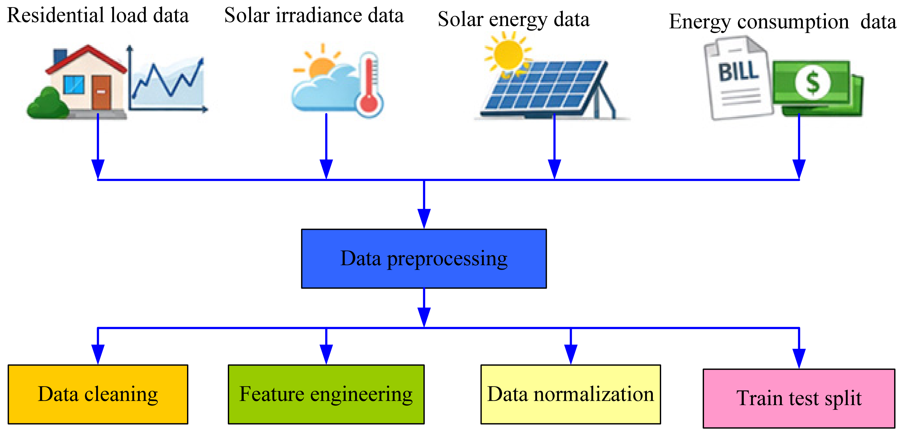
The dataset used in this study is obtained from a residential building equipped with a PV system in Durban, South Africa. The dataset consists of four key variables such as residential electrical load demand, solar irradiance, solar energy generation and electricity consumption. The datasets are directly related to residential energy management and forecasting. The above-mentioned variables are utilized in the study because they can capture demand-side and supply-side characteristics of the residential energy system. At the same time, the variables can provide the necessary information for forecasting of energy demand, solar irradiance, renewable energy generation and electricity costs under TOU tariff structures. The overview of the dataset description and time-based variables adopted in the study is presented in Figure 1.

Dataset Design

The dataset is designed to support the development and evaluation of ML models for forecasting residential energy system. This objective can be achieved by constructing a multivariate time-series dataset and using variables collected from a residential building equipped with a photovoltaic system in Durban, South Africa. Datasets from the site are recorded at an hourly resolution over a three-month period. The datasets produce a continuous series of observations that are appropriate for applications involving short-term forecasting. The hourly interval is selected in the study in order to observe the stochastic nature of residential electrical usage and solar energy system performance while maintaining time-based characteristics such as daily cycles, peak, standard and off-peak demand periods, weekday and weekend variations and fluctuations in solar resources. The dataset is a time series arranged in chronological order where observations are kept in their original temporal order during pre-processing, model development and evaluation to preserve the integrity of the forecasting problem. The historical observations are used in the study to predict future values and prevents information leakage during model training. The dataset is designed to capture the interactions between energy demand, solar resource variability and electricity consumption behaviour under realistic operating conditions. The three-month dataset used in the study contains sufficient temporal diversity to evaluate forecasting performance and assess the effectiveness of the proposed machine learning models. The dataset can be used as basic inputs for investigating residential energy forecasting and cost prediction in a smart energy management context.

2.2. Data Collection

Data collection is used in the study for gathering pertinent datasets that characterize electrical energy consumption, solar energy resources and environmental conditions [32]. The real-time datasets used in the study are obtained from residential energy consumption and solar generation systems in Durban, South Africa. The data collected from the residential building are integrated to form a multivariate time-series dataset that comprise hourly observations over a specific period of time. The hourly temporal resolution allows the dataset to capture significant operational characteristics of the residential energy system such as daily load fluctuations, variations in solar resources, changes in power output of the PV system and dynamic electricity consumption behaviour. The dataset contains useful time-based information that can be helpful in the development of precise forecasting models. The sequential associations in the time-series dataset are sustained by keeping all observations in their original chronological order during data preprocessing, model development and performance assessment. Hence, no random shuffling to guarantee that past observations are the only ones used to forecast future values. This method can be used for realistic evaluation of the forecasting models under real-world operating settings and prevent information leakage.

2.3. Data Preprocessing

Data preprocessing is crucial for development of accurate forecasting models of residential energy systems. It is an essential step that is utilized in this study to prepare the raw datasets for machine learning forecasting of residential electricity loads, renewable energy generation and electricity bills [33]. The datasets include hourly residential load consumption from smart metres, solar irradiance, renewable energy output data and household energy usage for electricity bill estimations [34]. The preprocessing steps implemented in this study are data cleaning, feature engineering, data normalization and data splitting. The data preprocessing diagram that illustrates the proposed framework is presented in Figure 2. The structure describes the steps used on the raw dataset to improve feature representation, increase data quality and make the data ready for model training.

2.3.1. Data Cleaning

Data cleaning is carried out in the study as the initial step of preprocessing process in order to guarantee the accuracy and consistency of the home energy dataset before model development. Data cleaning is the process of identifying and handling missing values, eliminating duplicate records, fixing discrepancies and identifying outliers resulting from sensor malfunctions or data collecting problems. This can offer a strong foundation for feature engineering, normalization and development of forecasting model within the domestic energy system. The missing observations are detected by exploratory data analysis and handled using suitable interpolation methods to maintain the sequential continuity of the time-series data. The duplicated records can be removed to avoid bias and duplication in the learning process. The consistency checks are carried out in the research work to certify that all variables are characterized in consistent units and fall within allowable measurement bounds. This approach can be used to increase the quality of the dataset and reduce the number of inaccurate data points. The data cleaning is performed in the research work to ensure that the dataset is accurate, comprehensive and suitable for feature engineering, normalization and forecasting model development.

2.3.2. Feature Engineering

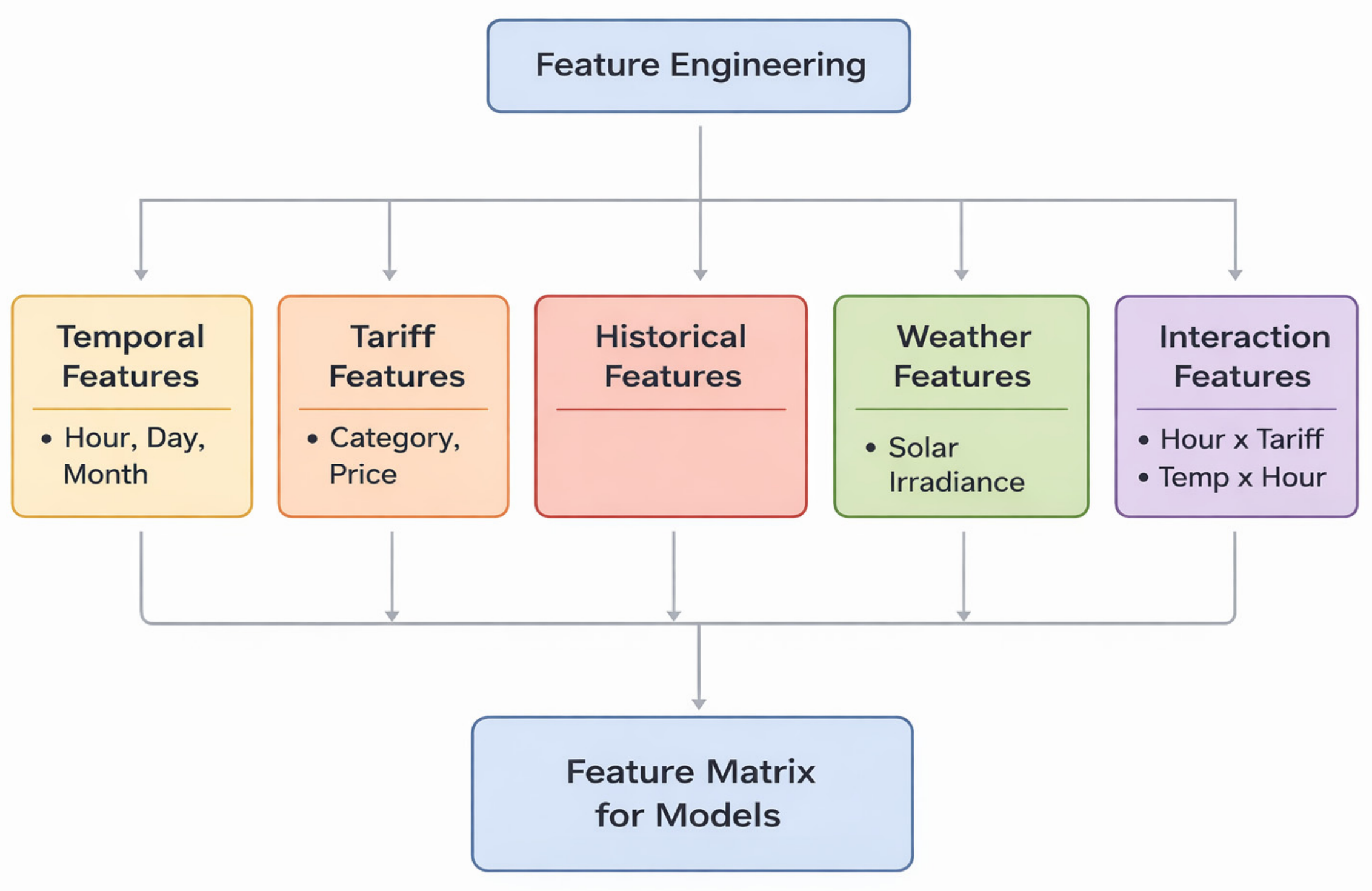
Feature engineering is a crucial stage in ML that allows the transformation of raw data into informative features to improve the predictive capability of forecasting models [10]. The engineering features are used as inputs to the ML models to achieve a highly accurate forecasting of load demands, solar irradiance, solar generation and electricity costs by extracting representative temporal and operational characteristics from the original dataset [35]. The feature engineering is presented in Figure 3 to demonstrate the transformation of unprocessed datasets into processed input variables for ML models. The complete three-month hourly dataset is first divided chronologically into training and testing subsets in order to prevent information leakage. The training dataset is used exclusively for all future feature engineering processes such as correlation analysis, feature selection, multicollinearity assessment and feature importance estimation. The independent test dataset is not utilized for feature selection, model training, or hyperparameter optimization; rather, it is only employed to assess the prediction performance of the forecasting models. Feature selection procedures such as Pearson correlation analysis, Variance Inflation Factor (VIF) analysis and model-based feature importance estimation are performed exclusively on the training partition after the chronological train/test split. The dataset is structured to increase the predictive competence of the forecasting algorithms through data cleaning, time-based feature extraction, feature transformation and selection of features [36]. The components of feature engineering are responsible for improving data quality and extracting informative features that enhance model performance.
The feature selection is performed using a multi-stage procedure on the training dataset. The procedure of feature selection consists of correlation analysis, feature importance ranking and multicollinearity assessment. First, Pearson correlation coefficients are computed between each input variable and the target outputs. Features with weak correlations (|r| < 0.1) are considered non-informative and excluded. Second, feature importance scores are computed using the training data to quantify the contribution of each feature to reduce prediction error. Features that consistently showed negligible importance across the trained models are deleted. Third, the VIF is used to evaluate multi-collinearity among the preserved features. Variables with VIF values greater than 10 are removed to eliminate redundant information and improve model stability. Based on abovementioned criteria, some indices such as solar irradiance, historical load demand, photovoltaic power output and TOU tariff are retained. While, redundant temporal variables and auxiliary sensor measurements are excluded due to weak correlation, low importance scores and high multicollinearity. The selected features obtained from the training data are subsequently used as inputs to the RF, GBR, XGBoost, DBN, RVFL, MLP and hybrid ensemble models.

2.3.3. Data Normalization

Data normalization is used to remove scale disparities among the input variable quantities and to increase the stability of the forecasting models. The residential energy datasets are measured in different units. Therefore, it is imperative to normalize the data into the same range because the collected variables have numerous numerical ranges and units. Data normalization is implemented in the study to ensure that features that have large magnitudes are not allowed to control the learning process. This procedure can be used to facilitate the convergence of ML algorithms. In the current study, the minimum to maximum normalization technique is employed to convert each variable to the same range of (0, 1) and standardize the variables. The normalization of the parameters is obtained solely from the training dataset and then applied to the testing and validation datasets to avoid information leakage. To preserve the integrity of the forecasting process, future information must not be incorporated in the model development.

2.3.4. Chronological Train, Validation and Test Strategy

The processed dataset can be partitioned into training, validation and testing subsets by utilizing a chronological train, validation and test strategy to sustain time-based consistency and prevent information leakage from future observations. The models are trained on the training data set and their parameters are optimized by the correlations between the input and output variables. This separation minimizes the risk of overfitting and enables a reliable evaluation of forecasting accuracy. The dataset is partitioned using a chronological train, validation and test strategy to preserve the temporal structure of the forecasting problem. The dataset is arranged in ascending chronological order and partitioned sequentially into three subsets. Specifically, 70% of the observations are allocated to the training set, 15% to the validation set and the remaining 15% to the testing set. The validation and testing datasets are placed in consecutive sequence after the initial observations for training. The strategy can be used to prevent information leakage and provide unbiased assessment performance of the model using future unseen data. The accuracy of the forecasting findings reported in this work are enhanced by the use of preprocessing techniques and the maintenance of chronological sequence. The accuracy of the forecasting findings reported in this work has been attributed to the use of preprocessing techniques and the maintenance of chronological sequence.

2.3.5. Training and Validation Procedure

The training and validation procedure is designed to ensure robust model development, prevent overfitting and provide an unbiased assessment of forecasting performance. The training dataset is used to train the RF, GBR, XGBoost, DBN, RVFL and MLP models after data partitioning. The aim of this phase is to find the fundamental connections between the input variables and the associated forecasting targets. The validation dataset is used to assess the performance of the model during development and optimize model configurations. The validation procedure is also used to compare the performance of the individual forecasting models and to determine the weights assigned to each model within the proposed hybrid ensemble framework. Model performance during training and validation is assessed using multiple evaluation metrics. These metrics provided complementary measures of forecasting accuracy and generalization capability. The model training is separated from validation and preserving the chronological order of observations to reduce the risk of information leakage, minimize the likelihood of overfitting and ensure that model optimization is performed using only historical data.

2.3.6. Hyperparameter Selection

Hyperparameter selection is performed to optimize the predictive performance and generalization capability of the forecasting models. Hyperparameters for all forecasting models are selected using the validation dataset. It is conducted using the validation dataset after the dataset is chronologically partitioning into training, validation and testing subsets. The test dataset is reserved exclusively for final model evaluation. No information from the test data is used during model development, hyperparameter tuning and ensemble construction. This procedure prevents information leakage and provides an unbiased estimate of model generalization performance. The reported test performance accurately reflects the generalization capability of the proposed forecasting framework on unseen data. The selected hyperparameters improve the reliability and robustness capability of the proposed forecasting framework.

2.4. Forecasting Models

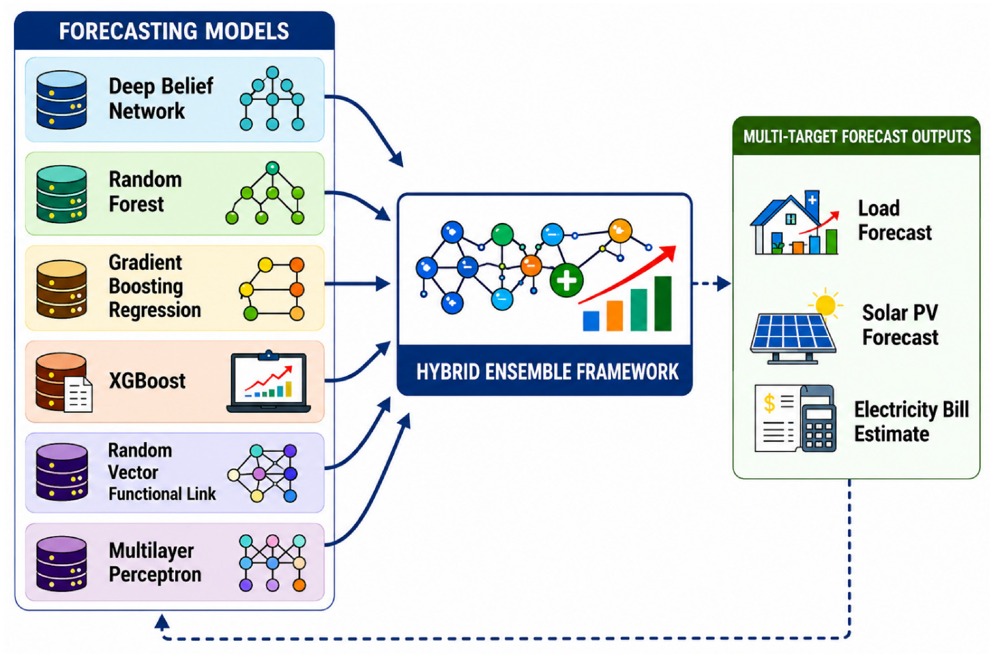
Forecasting models are statistical, DL and ML techniques that can be used in an energy management system to predict future values based on historical data trends and correlations among variables [35]. The models can predict future results by using patterns they have learned from past data. Forecasting models are used in the power system to predict solar irradiance, load demand, wind speed and electricity bills [32]. This study proposed machine learning models such as DBN, RF, GBR, XGBoost, RVFL, MLP and hybrid ensemble models for residential energy forecasting. These models are utilized in the study to complement the strengths and weakness of one another to capture nonlinear and stochastic patterns in load demand, electricity cost and renewable energy generation as shown in Figure 4.

2.4.1. Random Forest

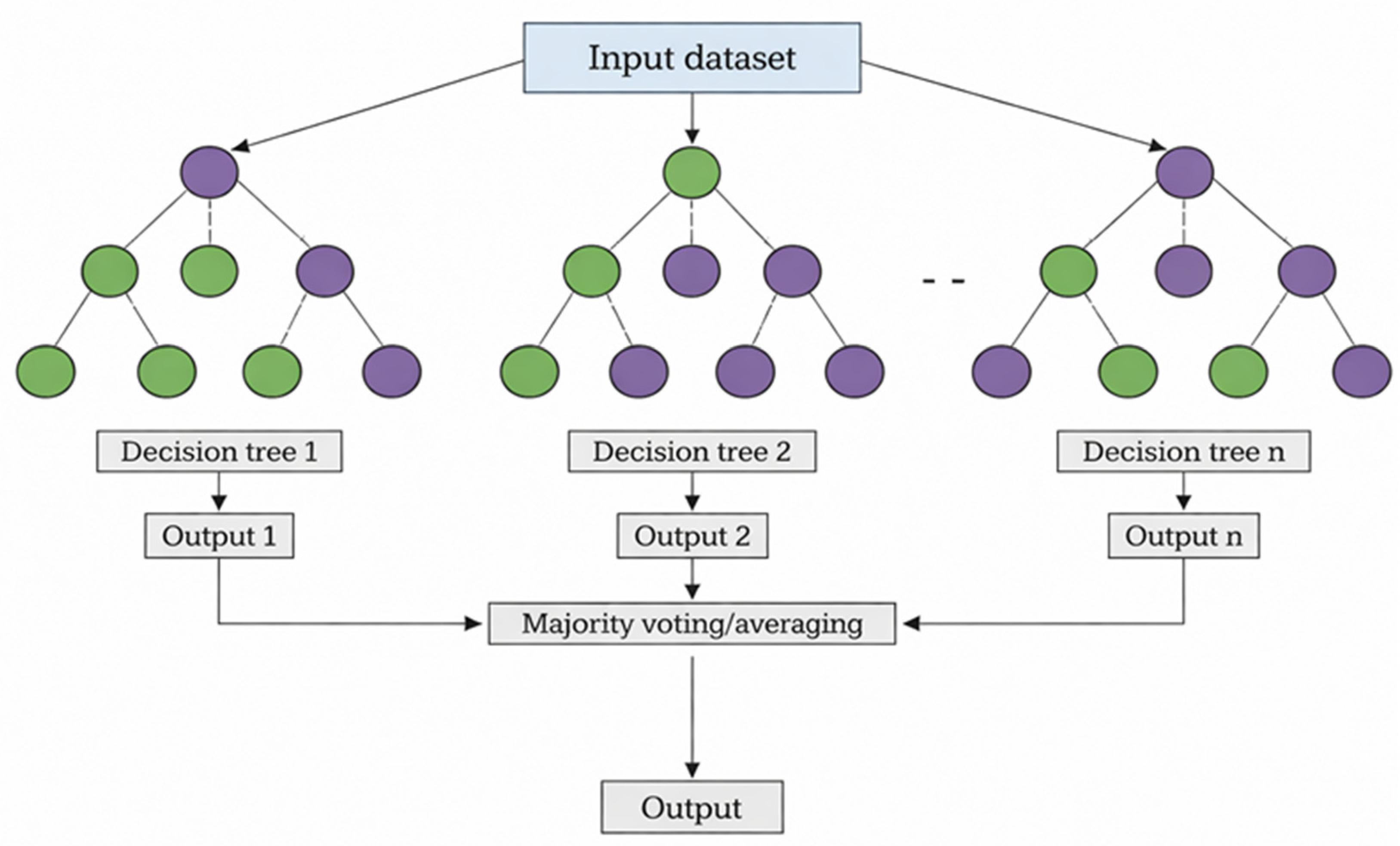
Random forest is a model that can be utilized to improve the prediction accuracy using multiple decision trees. The predictions of multiple decision trees are combined by RF to produce accurate and stable results [37]. The model consists of weak learners (decision trees) that can work together to form a strong predictive model. Bootstrap sampling is used to train each tree on a randomly chosen part of the dataset and random feature selection guarantees variation among the trees [35]. The RF model has several key components that work together to improve prediction accuracy and robustness as shown in Figure 5. RF can be used to enhance prediction reliability of the residential energy forecasting [38]. The regression prediction can be expressed in Equation (A1) of Appendix A as [39].

2.4.2. Gradient Boosting Regression

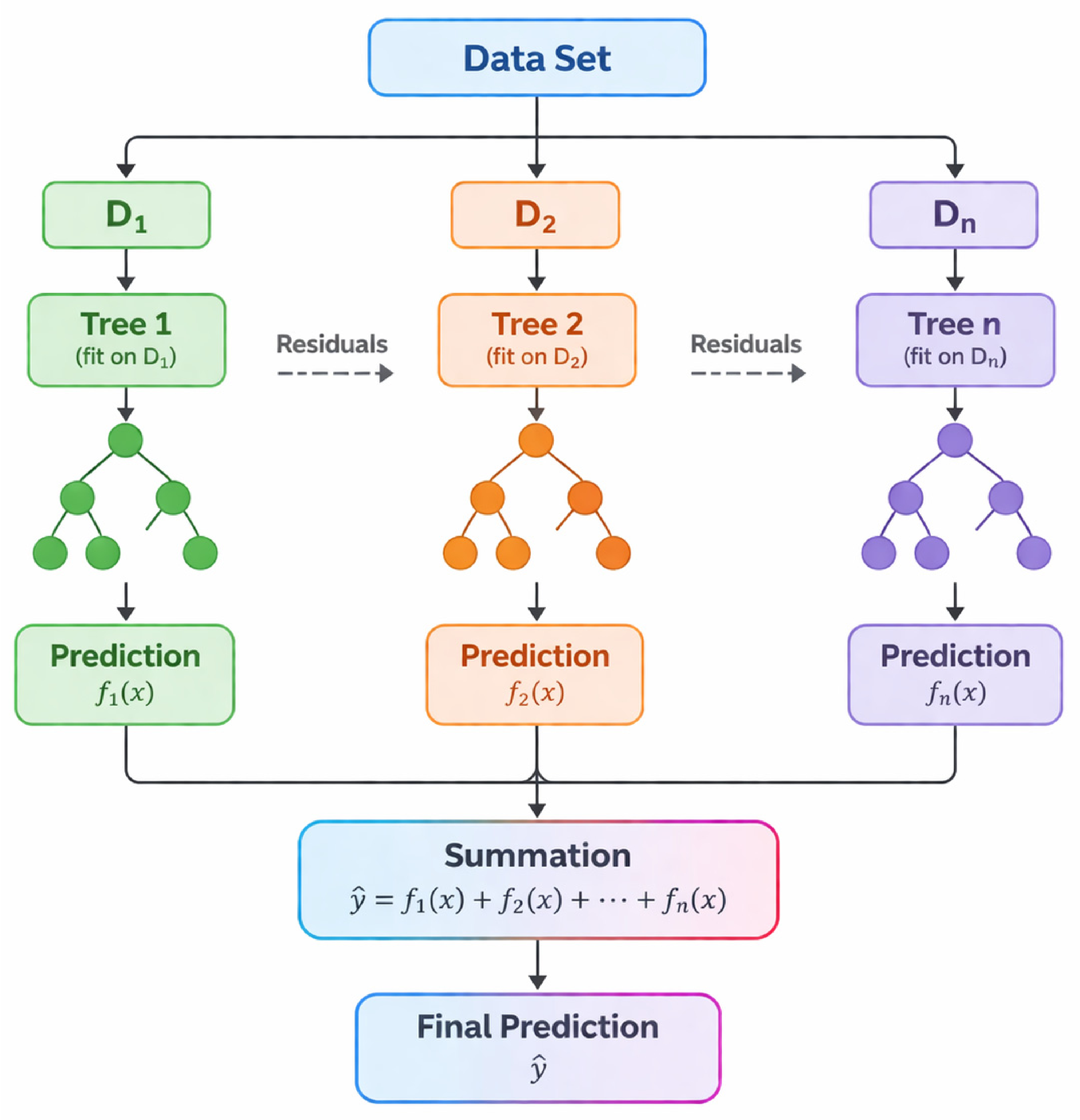
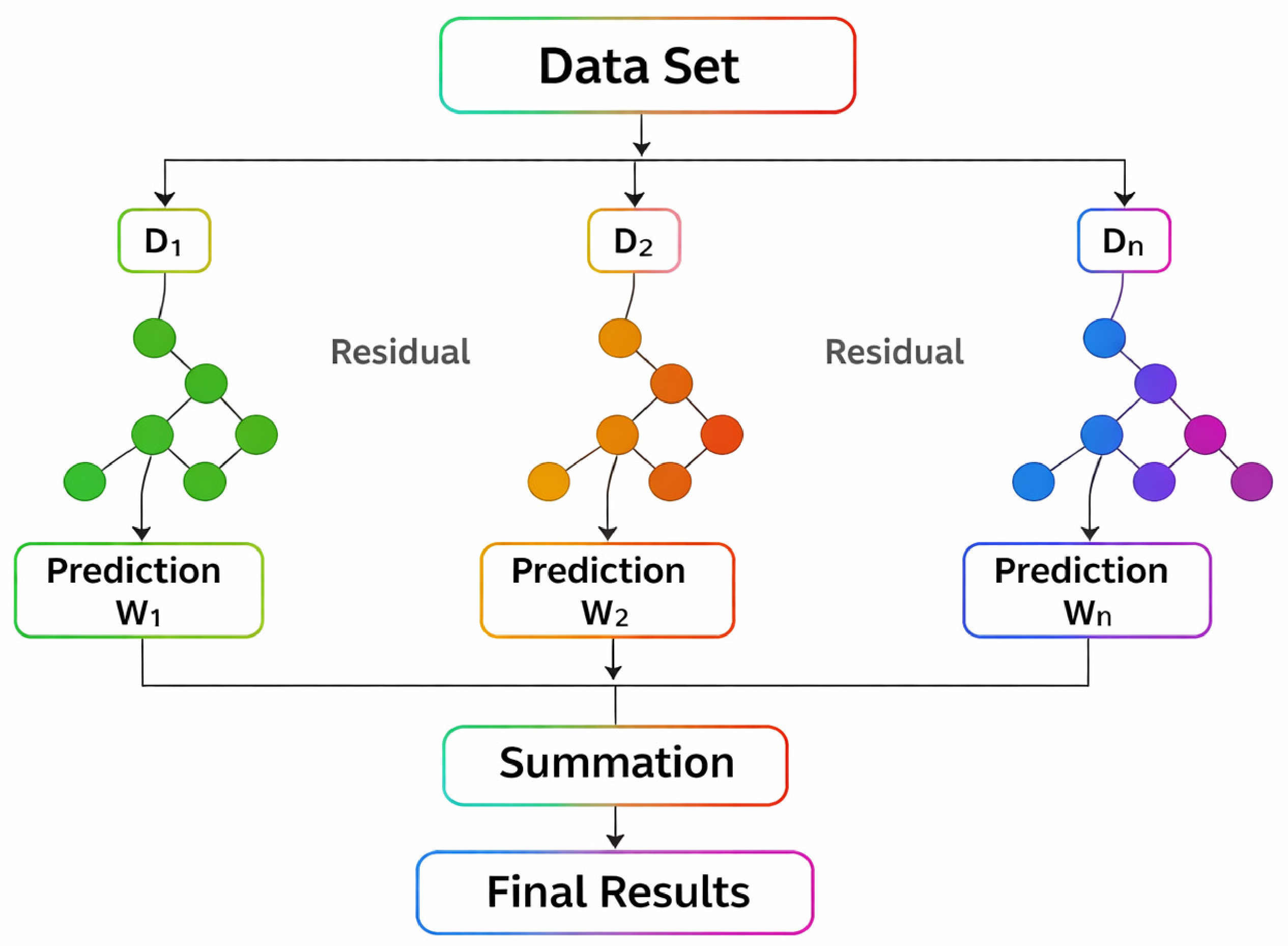
Gradient boosting regression is a technique that can be used to improve predictive performance by combining weak learners and minimizing errors using gradient descent [40]. It is globally utilized for renewable energy generation forecasting, load demand prediction, financial modelling, price estimation and predictive analytics owing to its strong accuracy and ability to model complex relationships. The architecture of gradient boosting regression is presented in Figure 6. GBR is a machine learning technique that builds a sequence of weak learners where each subsequent tree corrects the errors of the previous trees [41]. It can be used in residential energy forecasting to model the relationship between input variables. The prediction of GBR can be mathematically expressed in Equation (A2) of Appendix A as [42].

2.4.3. Extreme Gradient Boosting

Extreme gradient boosting is an effective ML model that can be used to increase conventional gradient boosting through regularization, optimized computation and improved tree construction approaches [43]. The architectural design of XGBoost with multiple components is shown in Figure 7. XGBoost is the best choice for complex forecasting problems due its strong predictive capability and scalability. The model has become widely adopted in forecasting and predictive analytics due to its ability to manage large datasets, missing values and complex feature interactions. In residential energy forecasting, it can be effectively captured relationships that exist between weather conditions, time variables and household consumption behaviours [44]. It is widely used in time-series forecasting, load prediction, renewable energy forecasting and electricity price prediction. The prediction of the XGBoost model is presented in Equation (A3) of Appendix A as [45].

2.4.4. Deep Belief Networks

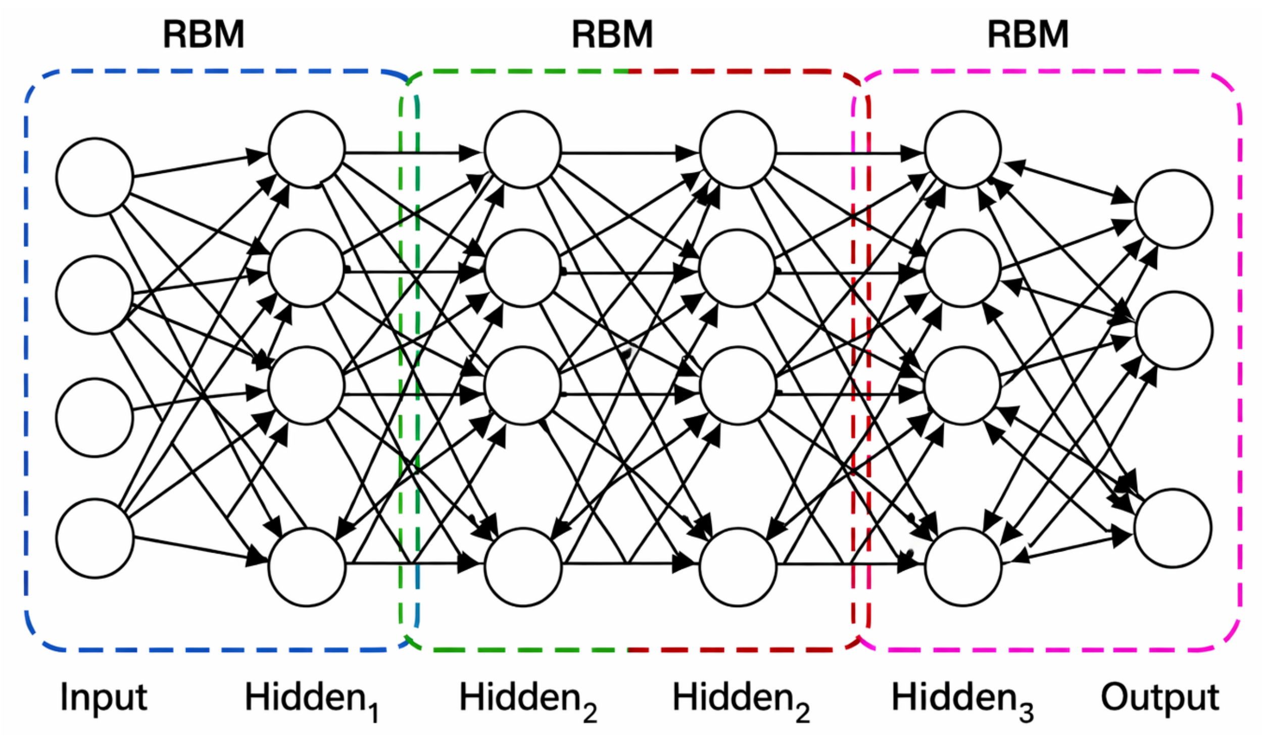
Deep belief networks are deep learning architecture that are capable of learning hierarchical feature representations from complex datasets [46]. These networks perform unsupervised feature learning by extracting hierarchical representations from complex datasets. They can increase the forecasting accuracy of load demand and renewable energy generation by using learning deep representation. DBNs can effectively capture hidden patterns and nonlinear relationships within data by stacking multiple restricted Boltzmann machines (RBMs). DBNs can be useful for latent patterns in high-dimensional energy datasets such as the relationships between weather conditions, solar radiation and electricity demand [47]. A DBN consists of several layers as shown in Figure 8. Each hidden layer is trained using a RBM that learns features from the previous layer. The prediction of DBN model can be expressed in Equation (A4) of Appendix A as [48].
In this study, fout is implemented as the rectified linear unit activation function as expressed in Equation (A5) of Appendix A.

2.4.5. Random Vector Functional Link

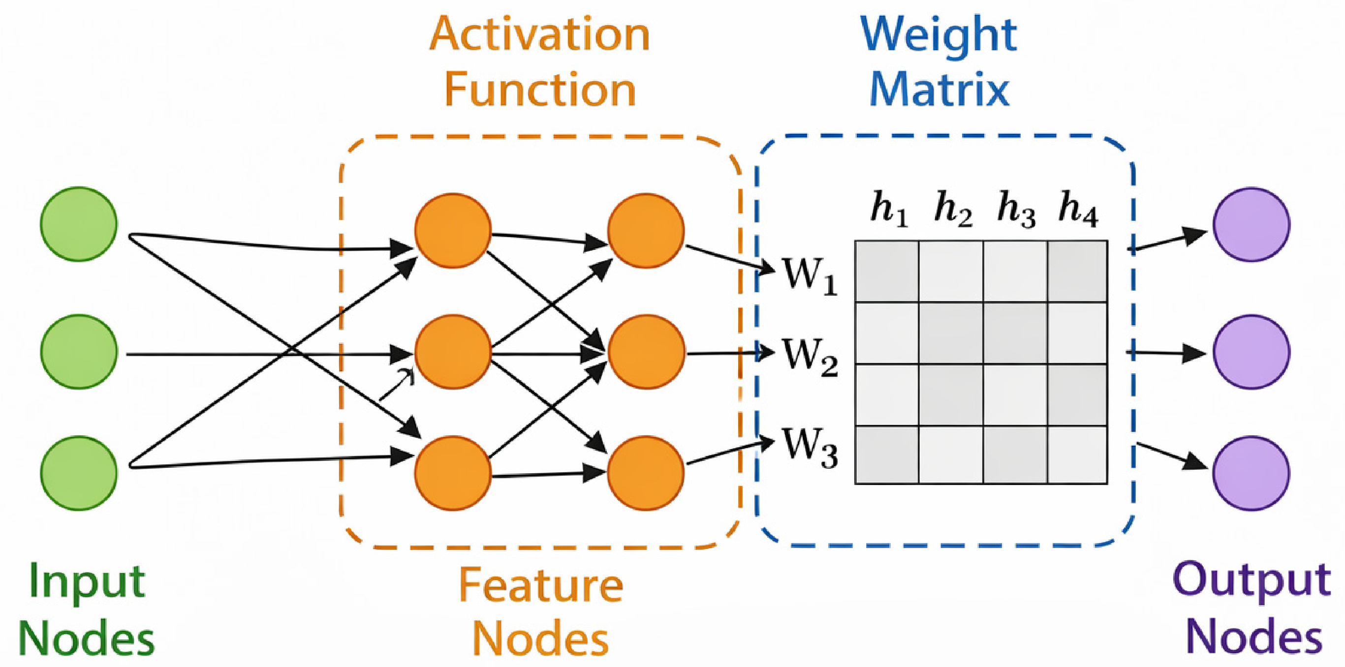
RVFL networks are single-layer feedforward neural networks in which the weights connecting the input layer to hidden nodes are randomly generated and fixed, while only the output weights are trained [49]. They can achieve fast learning and reliable predictive performance by combining randomized hidden layer transformations with direct input–output connections. They are fast to train and effective for regression tasks like energy load forecasting, renewable generation prediction and electricity price estimation. It can be seen from the RVFL architecture that it has direct links between the input and output layers to improve learning efficiency and reduce training complexity [25]. The RVFL network consists of several layers that can be used to improve learning stability and prediction accuracy as shown in Figure 9. The prediction of the RVFL model is presented in Equation (A6) of Appendix A as [25].
The random hidden layer output is expressed in Equation (A7) of Appendix A.

2.4.6. Multi-Layer Perceptron

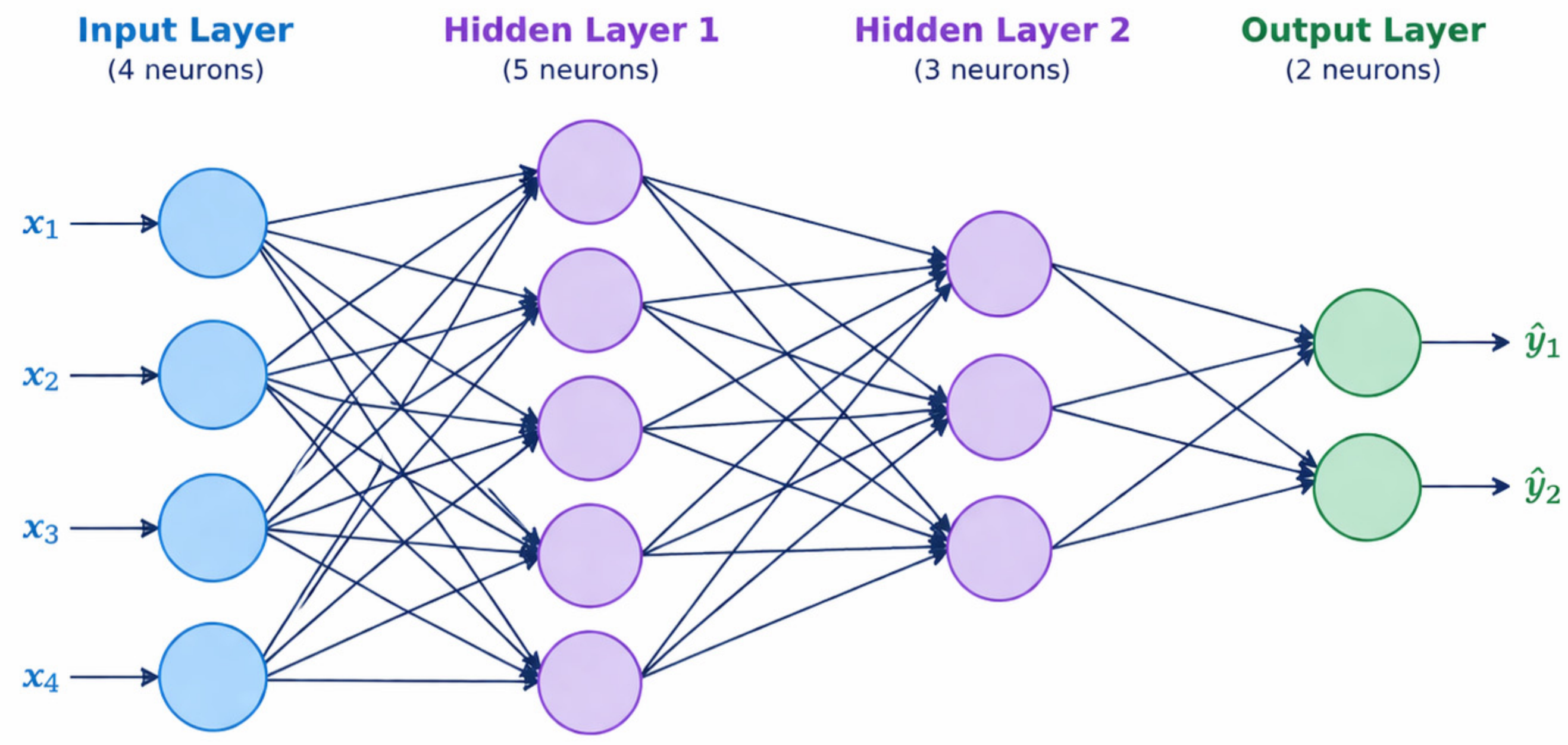
MLP is a neural network model that can be used for learning intricate nonlinear correlations of energy datasets. The MLP can be utilized in residential energy system and renewable energy generation data via application of several layers of interconnected neurons and back propagation learning [50]. MLPs are widely used for regression and forecasting tasks such as electricity demand and renewable energy prediction [51]. The MLP model is made up of several layers of interconnected neurons such as input, hidden and output layers as presented in Figure 10. The prediction of an MLP can be expressed in Equation (A8) of Appendix A.

2.4.7. Hybrid Ensemble Framework

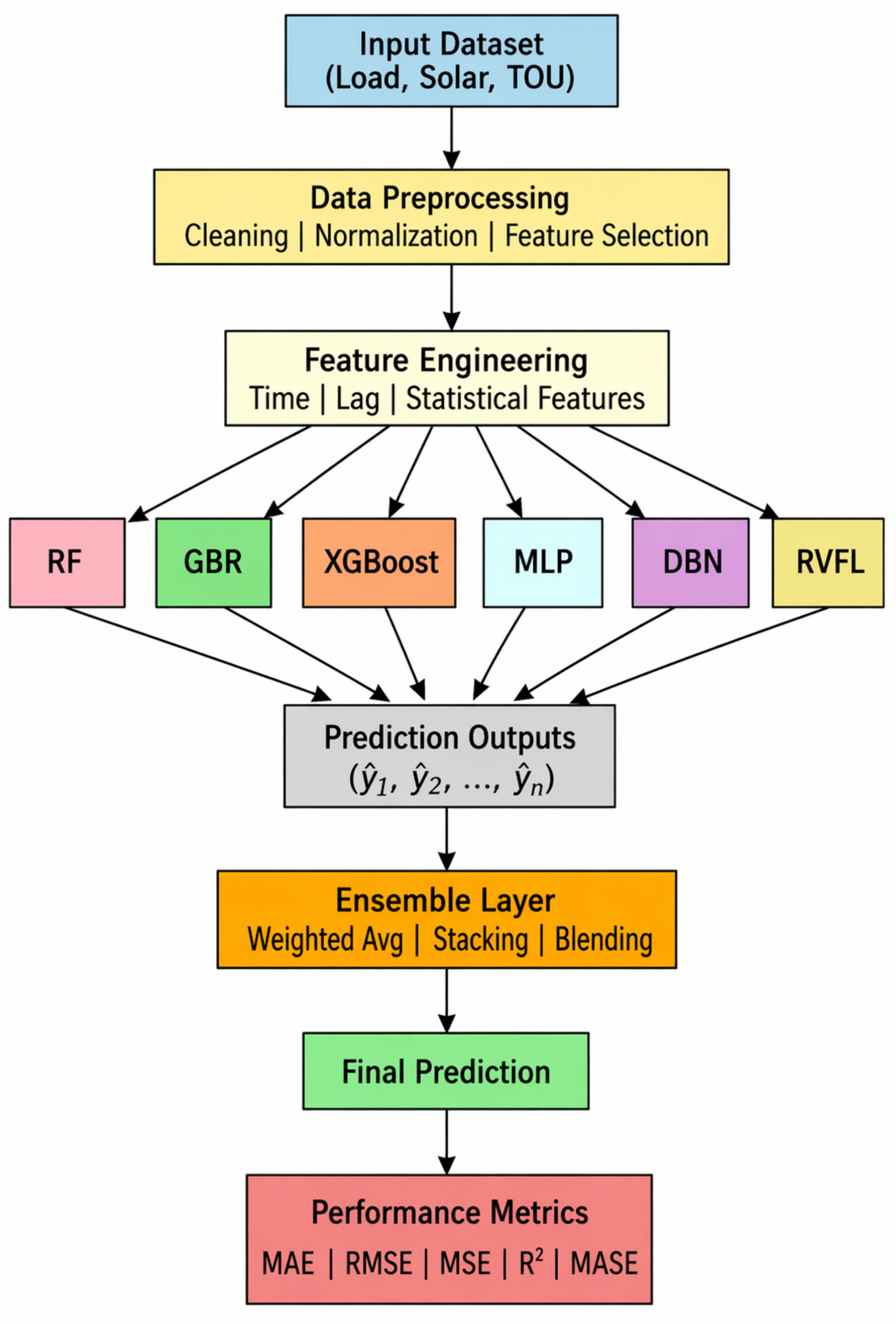
The hybrid ensemble framework is a powerful approach for energy forecasting which works by integrating multiple models such as RF, GBR, XGBoost, DBN, RVFL and MLP into a unified prediction system [52]. The hybrid ensemble learning combines the strengths of several algorithms to improve predictive performance and reduce model bias and variance instead of using just one model [53]. The framework can be used to enhance forecasting accuracy, stability and robustness by combining the strengths of diverse algorithms. In energy forecasting applications, hybrid ensembles are particularly effective because they can capture different data characteristics such as nonlinear relationships, stochastic variations and temporal dependencies [54]. The framework consists of several components performing specific functions within the forecasting process as shown in Figure 11. Each forecasting model acts as a base learner that can autonomously identify patterns from the input dataset and generate preliminary predictions. These predictions are subsequently combined through an aggregation mechanism to produce the final forecast output. It provides the final estimated values that can be used for energy management and decision-making. The construction of the hybrid model consists of three major stages such as individual model development, validation-based performance evaluation and ensemble integration. The hybrid ensemble prediction can be expressed in Equation (A9) of Appendix A [55] when equal weights are used:
The weights are computed based on a composite performance score derived from MAE, RMSE, MSE, MASE and R2. It ensures that models with superior validation performance contribute more significantly to the final output. This adaptive mechanism enhanced predictive robustness by using the complementary strengths of machine learning models. The final ensemble prediction is obtained through a validation-driven weighted fusion strategy where contribution of each model is based on its predictive performance and the validation of datasets. The ensemble output is presented in Equation (A10) of Appendix A.
The weights must satisfy Equation (A11) of Appendix A.
The weights are derived from a composite validation performance score computed using multiple evaluation metrics such as MAE, RMSE, MSE, MASE and R2 to ensure robust and unbiased model fusion. For each model i, an aggregated error score is expressed in Equation (A12) of Appendix A.
R2 that represents goodness of fit is incorporated as a corrective factor as shown in Equation (A13) of Appendix A.
The normalization weighting assigned to each model is computed using inverse scoring scaling as presented in Equation (A14) of Appendix A.

2.5. Evaluation Metrics

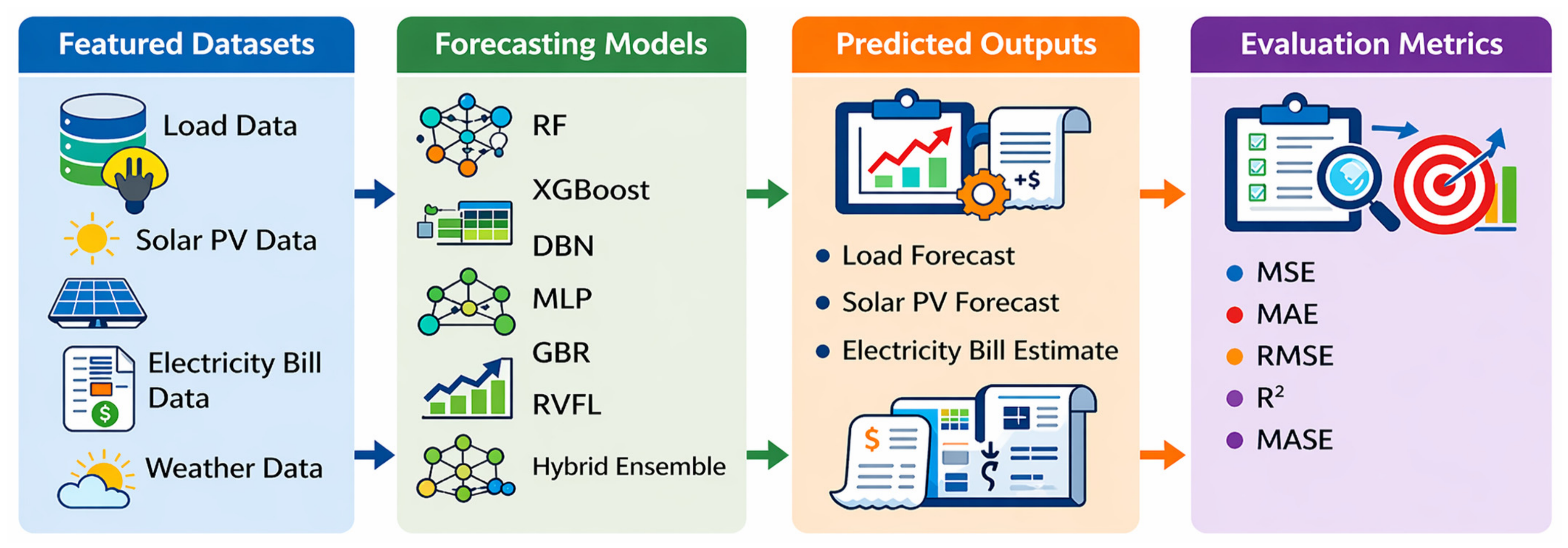
Evaluation metrics can be used to assess the performance of each model by comparing its predicted values with the actual observed values. They can be used to determine the accuracy, reliability and suitability of models for forecasting in real-time applications [56]. The accurate evaluation of forecasting techniques can be used to quantify their predictive performance by critically comparing several algorithms. The performance of the models is assessed in this study by utilizing globally accepted metrics such as RMSE, MAE, R2, MSE and MASE. The evaluation of model performance is carried in the study by using input dataset, forecasting models, predicted outputs and evaluation metrics as presented in Figure 12. The figure illustrates how the datasets that consist of load demand, solar irradiance and electricity consumption are fed into the forecasting models such as GBR, RF, XGBoost, RVFL, DBN and MLP. The predicted outputs of the system are evaluated using performance metrics to quantify the accuracy of the model. The following performance evaluation metrics are utilized in the study to select the best suitable model among several alternatives.

2.5.1. Mean Absolute Error

MAE is a measure that can be used to quantify the average magnitude of the errors between the predicted and actual values [56]. It is expressed in Equation (A15) of Appendix A as [46].

2.5.2. Root Mean Squared Error

RMSE is a statistical metric that can be utilized to quantify the average magnitude of prediction errors. This metric is useful for evaluating models where large deviations are critical such as peak load and solar generation forecasting [56]. RMSE is expressed in Equation (A16) of Appendix A as [46].

2.5.3. Coefficient of Determination

R2 is a statistical metric that can be used to measure the proportion of variance in the observed data explained by the predictive model [56]. The coefficient of determination is expressed in Equation (A17) of Appendix A as [46].

2.5.4. Mean Squared Error

MSE is a statistical metric that can be utilized to quantify the average of the squared difference between predicted and actual values. It can be used in energy forecasting to evaluate the accuracy of load demand, solar irradiance, wind speed and electricity bill predictions [56]. MSE can be estimated by using Equation (A18) of Appendix A [46].

2.5.5. Mean Absolute Scaled Error

MASE is a statistic measure used in time-series analysis to assess the accuracy of forecasting models [4]. MASE can be expressed in Equation (A19) of Appendix A.

2.6. Statistical Error Analysis

Statistical error analysis is the methodology assessment of the distribution errors produced by forecasting models based on their bias and accuracy. It can be used to assess the degree of deviation of predicted values from the observed values. The prediction error for each observation is defined as the difference between the actual and predicted values [12]. The prediction error can be expressed in Equation (A20) of Appendix A.

2.6.1. Mean Error

Mean error (bias) is a statistical measure used to evaluate the average deviation of predicted values from the corresponding observed values. A value close to zero indicates an unbiased model, while positive and negative values correspond to overestimation and underestimation [57]. It is expressed in Equation (A21) of Appendix A as [58].

2.6.2. Error Standard Deviation

Error standard deviation is a statistical measure that can be used to quantify the variability of prediction errors around their mean and reflect the consistency of model predictions [59]. It is expressed in Equation (A22) of Appendix A as [60].

2.6.3. Error Range

The error range a statistical measure that can be used to quantify the spread of prediction errors by identifying the minimum and maximum deviations between predicted and actual values. It reflects the extent of extreme prediction errors and overall spread. It is presented in Equation (A23) of Appendix A as [61].

2.6.4. Skewness

Skewness is a statistical metric that can be used to quantify the asymmetry of the error distribution around its mean. It can be expressed in Equation (A24) as [62].

2.6.5. Kurtosis

Kurtosis is a statistical measure that describes the peak and tail heaviness of the error distribution. Kurtosis is expressed in Equation (A25) as [62].

2.7. Overview of the Study Area

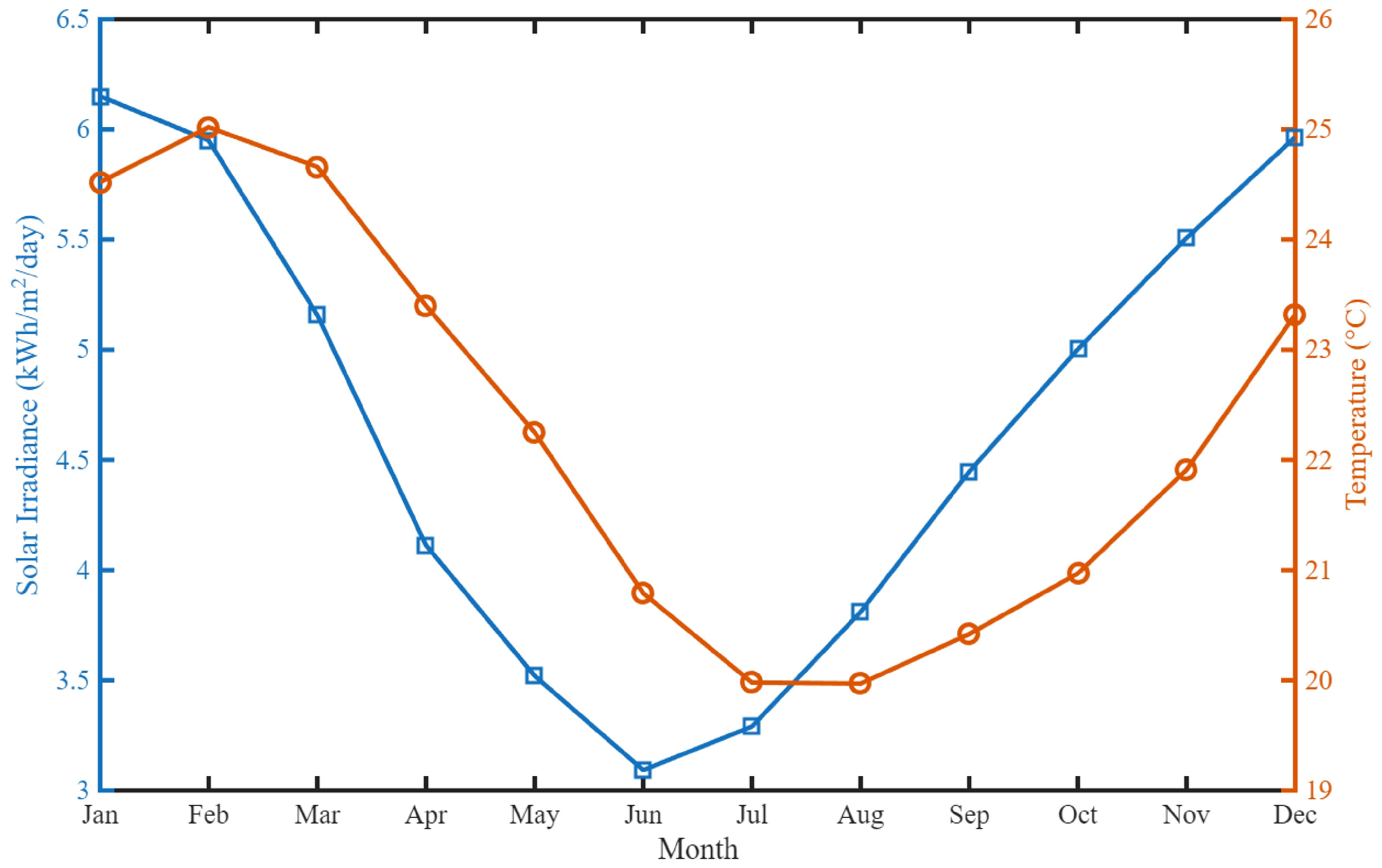
Durban that is located in the KwaZulu-Natal province of South Africa is selected as the location for forecasting of residential electrical load demand, solar irradiance, renewable energy generation and electricity costs under TOU tariffs [63]. Durban is one of the largest coastal cities in South Africa that is characterized by a rapidly growing population, expanding urban infrastructure and increasing electricity demand. The city is located on the Eastern coast of South Africa with geographical coordinates of 29.9° S latitude and 31.0° E longitude as shown in Figure 13 [64]. It is characterized by average temperature of 22–29 °C, annual average wind speeds of 3–4 m/s, average annual solar irradiance of 4.5–5.5 kWh/m2/day throughout the year [65]. These characteristics make Durban suitable for photovoltaic integration and solar forecasting studies. Eskom that used a combination of renewable and coal-based energy sources is the main provider of electricity to Durban, South Africa [66]. This study utilized ML models in conjunction with the TOU tariff to forecast electricity bills, solar energy generation and load demand. The monthly average temperature and solar irradiance characteristics of Durban obtained from the NASA POWER database are presented in Figure 14.
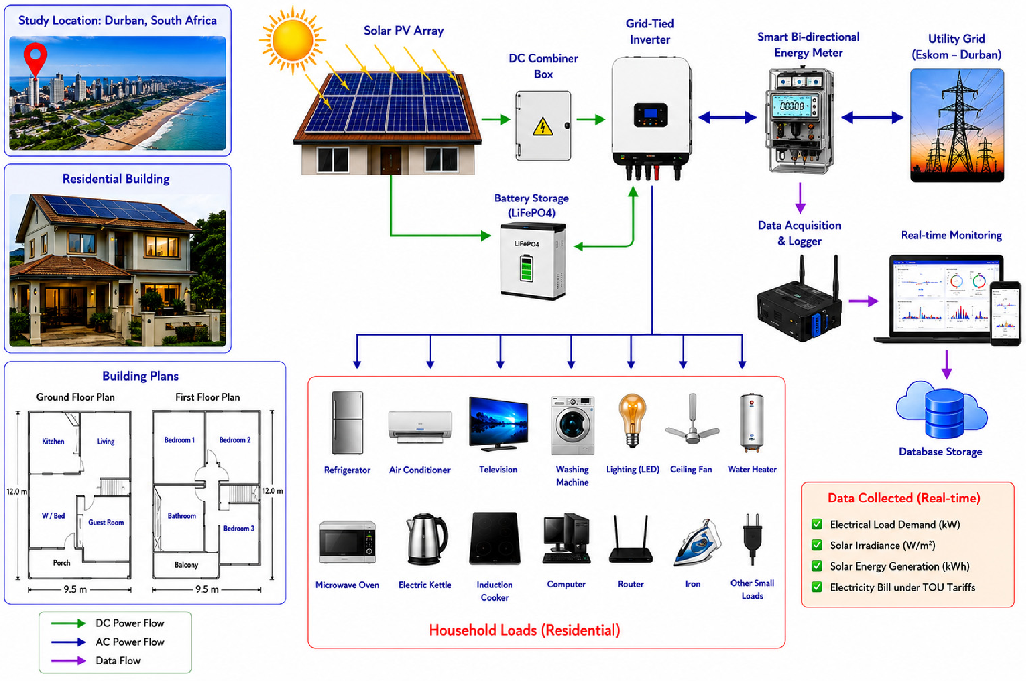
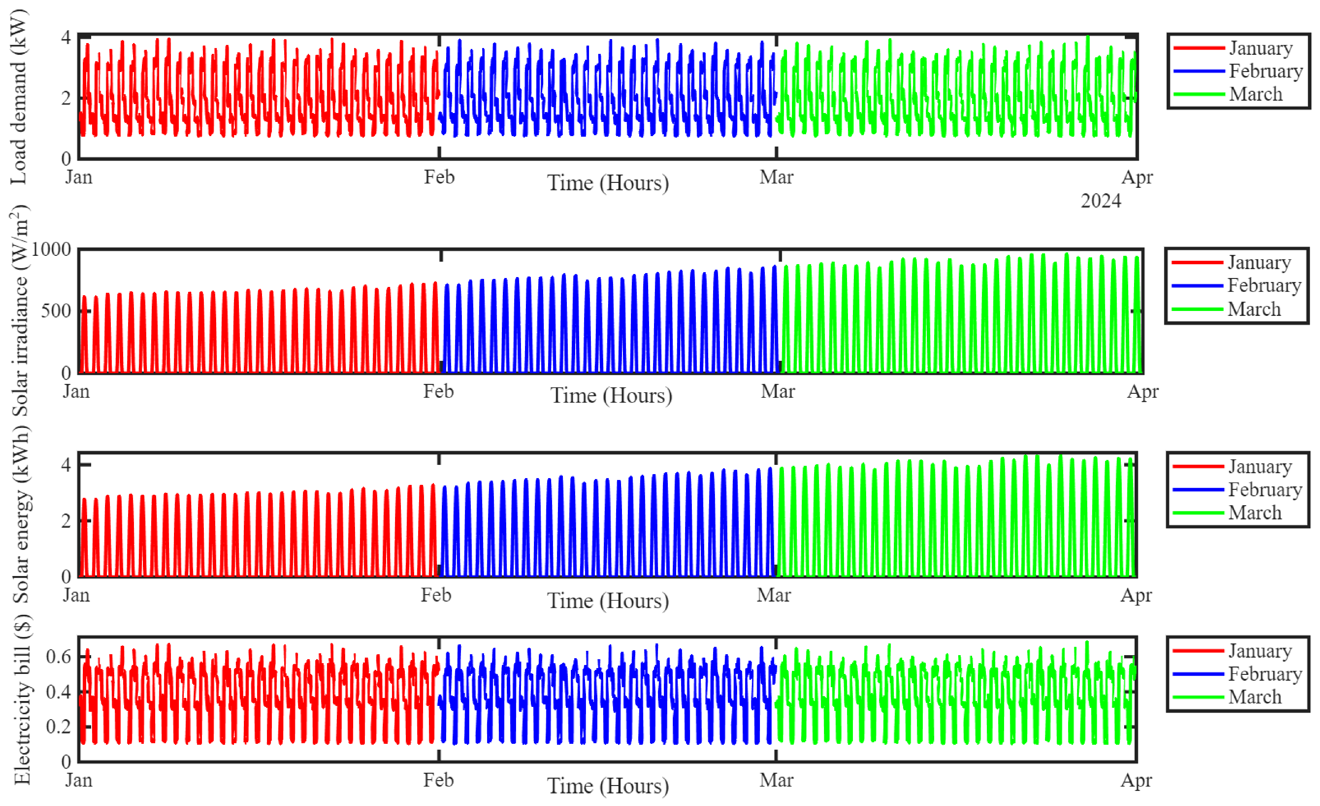
The dataset utilized in this paper is obtained from a residential building that is located in Durban, South Africa. The residential building considered in this study is a family residential structure with three bedrooms, one living room, kitchen, dining room, one guest room, one bathroom, one porch and one balcony as shown in Figure 15. The dataset used in this study is constructed from three months of historical observations for training and validating the forecasting models. The sampling frequency of the dataset is one hour, which corresponds to 24 observations per day. The dataset sizes for the months of January, February and March vary according to the number of days in each month based on an hourly basics. The hourly residential load demand, solar irradiance, solar energy generation and electricity consumption over the study period are presented in Figure 16. A three-month dataset is considered sufficient for this study because the objective is short-term residential energy forecasting using high-resolution hourly data. The dataset consists of residential load demand, solar irradiance and solar energy generation that can be used for assessment of the forecasting performance of the proposed machine learning models. This duration can provide adequate information for training and validating data-driven models. The model is optimized for short-term operational forecasting and transient decision-making within the investigated period. The model demonstrated excellent predictive accuracy but the limited temporal coverage did not capture the full spectrum of seasonal variability and long-term electricity demand patterns.

3. Results and Discussion

The simulation was conducted on MATLAB 2025b (MathWorks, Inc., Natick, MA, USA) using 12th Gen Intel (R) Core (TM) i5-1235U (1.30 GHz) with RAM of 8 GB, graphical card of 128 MB, storage of 500 GB and Windows 11. The results obtained from forecasting of residential load, solar irradiance, solar energy generation and electricity costs based on TOU tariffs of Durban, South Africa are presented in this section using the proposed models. The performance of each model such as RF, GRB, XGBoost, DBN, RFVL, MLP and hybrid ensemble models is assessed using multiple error metrics like MSE, RMSE, MAE, MASE and R2. The abovementioned performance indicators are simultaneously assessed using multiple approaches. The improved forecasting accuracy of MAE, RMSE, MSE and MASE is demonstrated by their lower values while higher values of R2 indicate a very strong correlation between the predicted and actual values. The interpretation of the models is presented in this section using model accuracy, error histograms and time series. The outcomes of the study are presented as follows.

3.1. Load Demand Forecasting

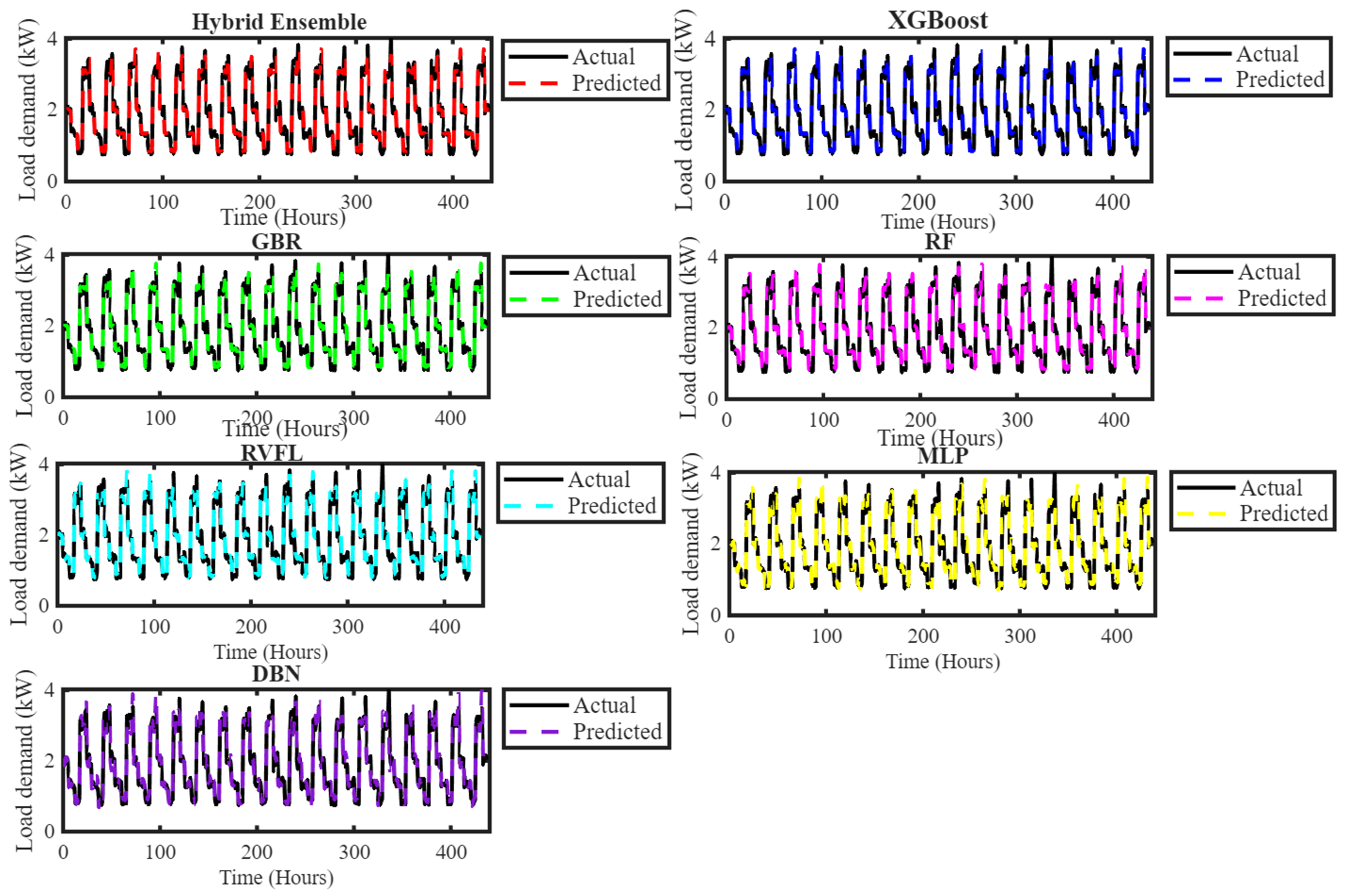
The performance evaluation of various models for residential electrical load demand forecasting of a residential building in Durban, South Africa is presented in this section. The models considered include RF, GBR, XGBoost, DBN, RVFL, MLP and hybrid ensemble. The forecasting accuracy of each model is assessed in the study utilizing MSE, RMSE, MAE, MASE and R2. The comparative analysis presented in Figure 17 shows that the abovementioned models can capture the temporal patterns of load demand and their predictive accuracies vary significantly based on their learning mechanisms. The output of the study as presented in Figure 17 illustrates how predicted load demand of each model tracked the actual residential load demand pattern. The performance of the hybrid ensemble is the best among all the models based on the ability of its prediction to perfectly overlap the actual load demand throughout the 430 h horizon. The high robustness and superior accuracy of ensemble hybrid has been attributed to hybridization of multiple models to reduce prediction errors and deviation and improve generalization. The prediction pattern of XGBoost closely followed the actual load pattern with small deviations based on its strong predictive capability. The performance of XGBoost is slightly below the hybrid model. The predictions of GBR and RF are less precise when compared to hybrid ensemble and XGBoost models. They have good alignment with actual load demand due to minor inconsistencies noticed at the peak points. The RVFL model has moderate performance to capture the pattern of the load demand with noticeable deviations at sharp peaks. The performance of the MLP and DBN models is the least among the seven models presented in the study due to it having the lowest accuracy and large deviation from the actual load demand. The hybrid ensemble model is the most suitable model for load demand forecasting applications in the study since it has achieved the highest level of accuracy and stability.
The statistical distribution of load demand forecasting errors is further analyzed using error histograms presented in Figure 18. The combined operation of these results provides a detailed assessment of prediction accuracy, variability and distributional characteristics. The error histograms reveal that all models produce errors that are cantered close to zero and indicate negligible systematic bias in load prediction. The distributions vary greatly amongst models in terms of their spread and shape. The distribution of the hybrid ensemble model is symmetrical and heavily concentrated around zero. This demonstrates the superior predictive accuracy and minimal deviation of the hybrid ensemble model when compared to XGBoost, GBR, RF, RVFL, MLP and DBN models. XGBoost and GBR models closely followed with a relatively narrow and symmetric error distribution to maintain strong central concentration. RF and RVFL models produced more noticeable tails and broader spreads to increase variability and reduce consistency and accuracy. The error distribution of the DBN and MLP models is the widest and the most irregular among all models owing to high dispersion and uncertainty and low reliability.
The statistical characteristics of prediction errors obtained from the evaluated models for load demand forecasting are presented in Table 1. The analysis consists of mean error, error range, standard deviation, skewness and kurtosis that can be used for comprehensive evaluation of the model’s accuracy, consistency and robustness. The mean error values for all models are observed to be very close to zero, this indicates that the models exhibit minimal systematic bias. The values of mean errors observed in the hybrid ensemble, XGBoost and GBR are −0.00013186, −0.00013880 and −0.00012515, demonstrating near-perfect unbiased predictions of the models. RF and RVFL models have negative mean errors of −0.0004371 and −0.001214, this indicates mild underestimation. MLP and DBN have positive mean errors of 0.00330350 and 0.00341770, with the tendency of overestimating the load demand. The error range and standard deviation serve as critical metrics for variability and consistency of model predictions. The hybrid ensemble has the lowest error range of 0.81093 and standard deviation of 0.11600 to demonstrate high concentrated errors and superior prediction stability of the model. Similarly, XGBoost and GBR demonstrate strong performance with low error range of 0.85361 and 0.97101 and standard deviation of 0.1221 and 0.14026. The RF, RVFL and MLP models exhibit relatively high error range of 1.1093, 1.2153 and 1.3868 and high standard deviation of 0.158, 0.18327 and 0.20994 to confirm their limitations in maintaining consistent predictive performance. DBN model has the highest error range of 1.64520 and standard deviation of 0.24741. The results obtained from the study indicate that ensemble and boosting-based models are more stable and reliable when compared to neural network-based models. The skewness values for all models are positive within the range of 0.27095 and 0.36438 to demonstrate slightly right-skewed error distributions. The hybrid ensemble has a balanced skewness of 0.3448 to illustrate a stable transition between peak and off-peak forecasting. The highest kurtosis value of 3.6505 of the RF models suggests a greater likelihood of extreme prediction errors. MLP and RVFL models have relatively lower kurtosis values of 3.4525 and 3.3586. The hybrid ensemble produced moderate kurtosis value of 3.6003 with the presence of outliers. The outcomes of the study demonstrate that the performance of the ensemble hybrid approach is better than other models due to its ability to reduce both bias and variance.
The performance evaluation of the forecasting models as presented in Table 2 provides critical insights into the accuracy and robustness capability of each approach in predicting residential electrical load demand. The hybrid model has the lowest MSE of 0.013425, MAE of 0.090522, RMSE of 0.11587 and MASE of 0.28023 and the highest R2 of 0.99344. The outcomes of the study clearly demonstrate that the hybrid model performed better than each individual model in every evaluation metric. XGBoost achieved relatively low MSE of 0.014875, MAE of 0.095286, RMSE of 0.12196 and MASE 0.29498 and high R2 of 0.98166. The performance of XGBoost is attributed to its sophisticated boosting mechanism and regularization competencies to avoid overfitting of load demand forecasting. The effectiveness of the GBR model as a robust technique for residential load demand forecasting is presented in Table 2. MSE of 0.019628, MAE of 0.10966, RMSE of 0.1401, MASE of 0.33947 and R2 of 0.9758 are attained by the model. This indicates a strong predictive capability with relatively low error margins. The performance of GBR is attributed to its sequential boosting mechanism. It can be seen from the results presented in Table 2 that the RF has consistent and reliable predictions with moderate accuracy in residential load demand forecasting. The model attained MSE of 0.024907, MAE of 0.12303, RMSE of 0.15782, MASE of 0.38086 and R2 of 0.96928. This indicates a reasonably good predictive capability, but its inability to effectively capture high variability and peak demand patterns limits its overall performance. The RVFL model demonstrates moderate and competitive performance in residential load demand forecasting. The RVFL model achieved MSE of 0.033513, MAE of 0.14381, RMSE of 0.18307, MASE of 0.44518 and R2 of 0.95867 to demonstrate a balanced trade-off between prediction accuracy and computational efficiency. The MLP model achieved MSE of 0.043986, MAE of 0.16601, RMSE of 0.20973, MASE of 0.5139 and R2 of 0.94576. The MLP model has moderate but relatively lower performance compared to hybrid ensemble, XGBoost, GBR, RF and RVFL approaches in residential load demand forecasting. The performance of the DBN model is the lowest among all evaluated models for residential load demand forecasting. It achieved MSE of 0.061083, MAE of 0.19359, RMSE of 0.24715, MASE of 0.59929 and R2 of 0.92467. The DBN model has limited effectiveness in residential load demand forecasting due to its higher error metrics and wider error distribution. The improvement of the hybrid model is compared with the best individual model in this study. The proposed hybrid model reduced RMSE from 0.112196 to 0.11587 when compared with the best individual model (XGBoost), this translates to a 5% reduction. Similarly, MAE reduced by 5%, MASE reduced by 5% and MSE reduced by 9.748%, while R2 increased from 0.98166 to 0.98344.
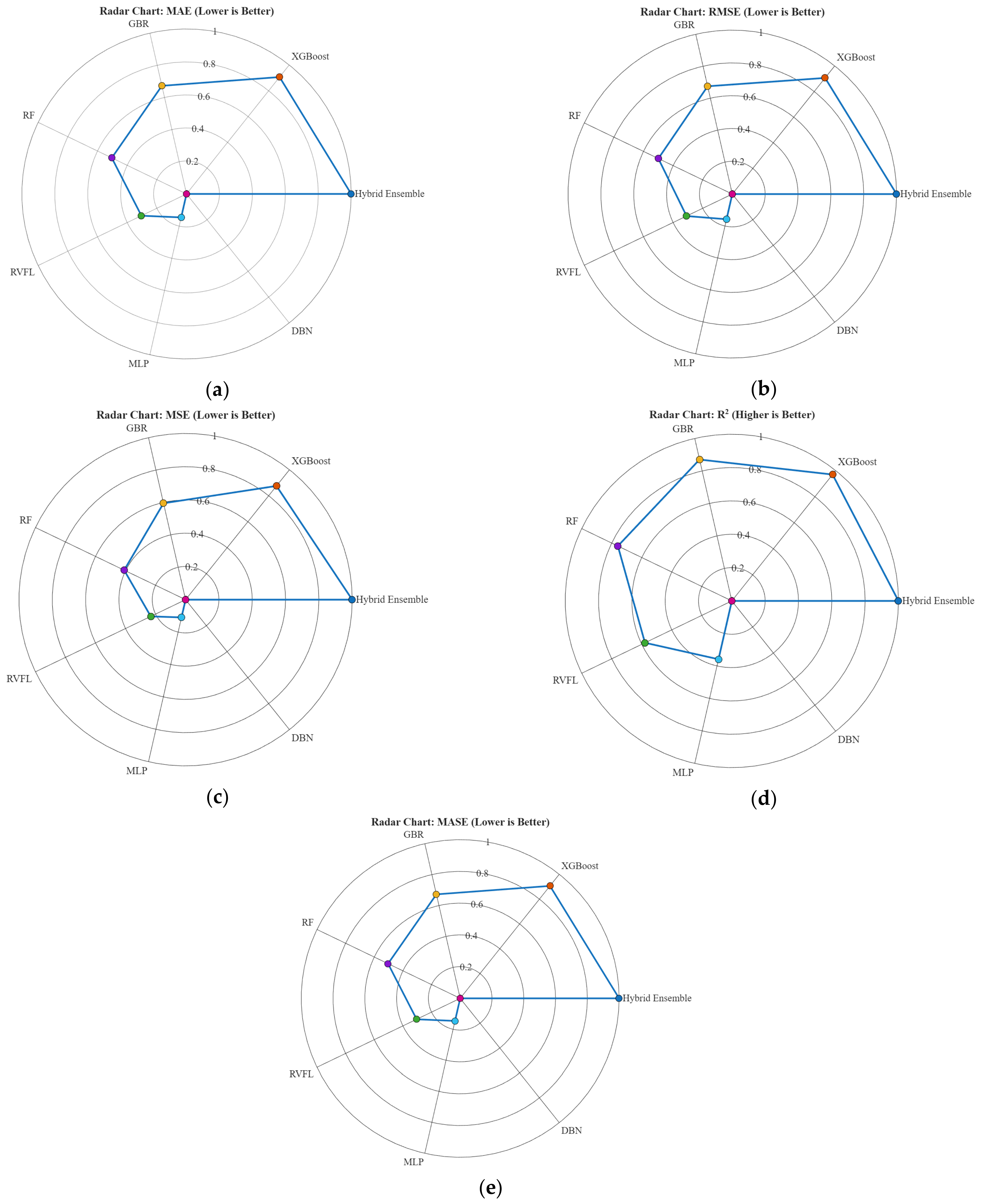
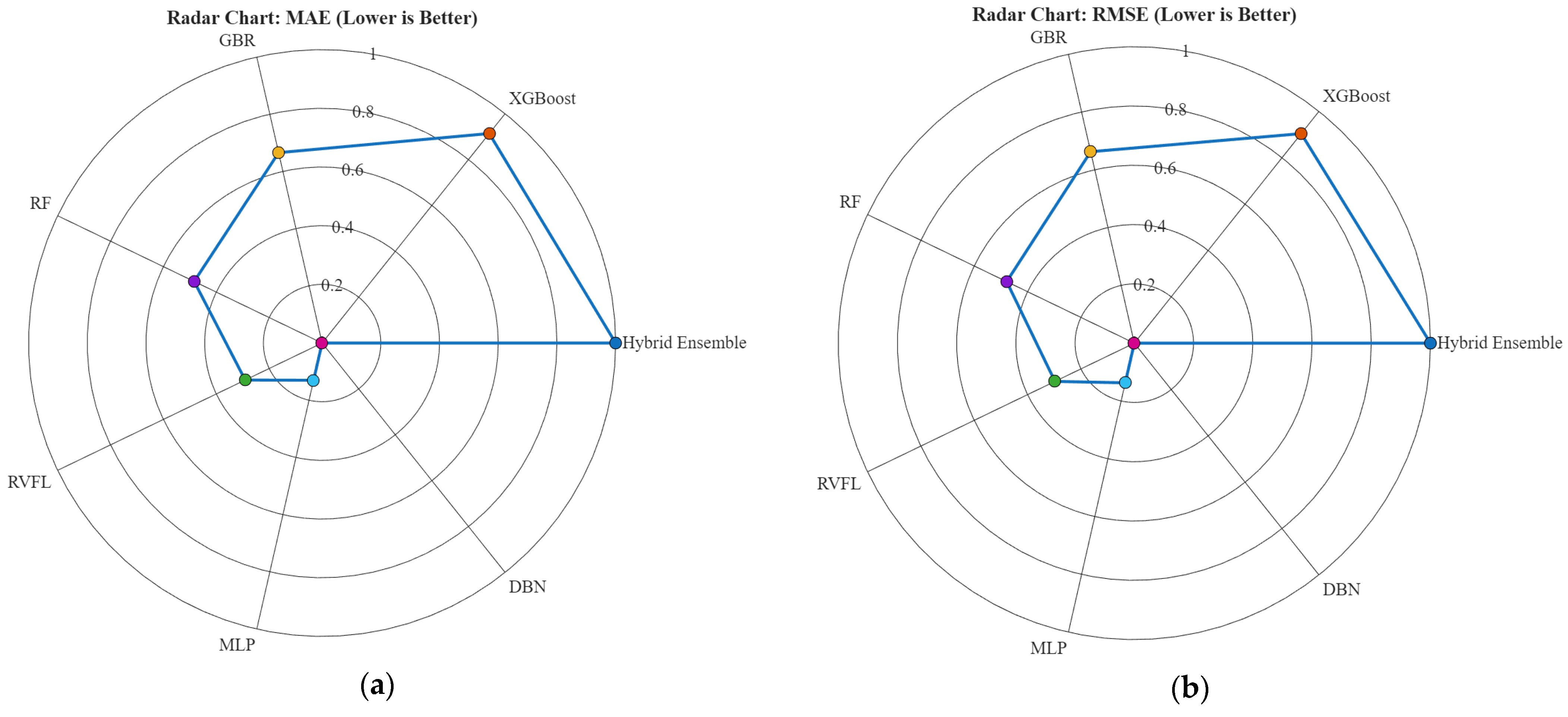
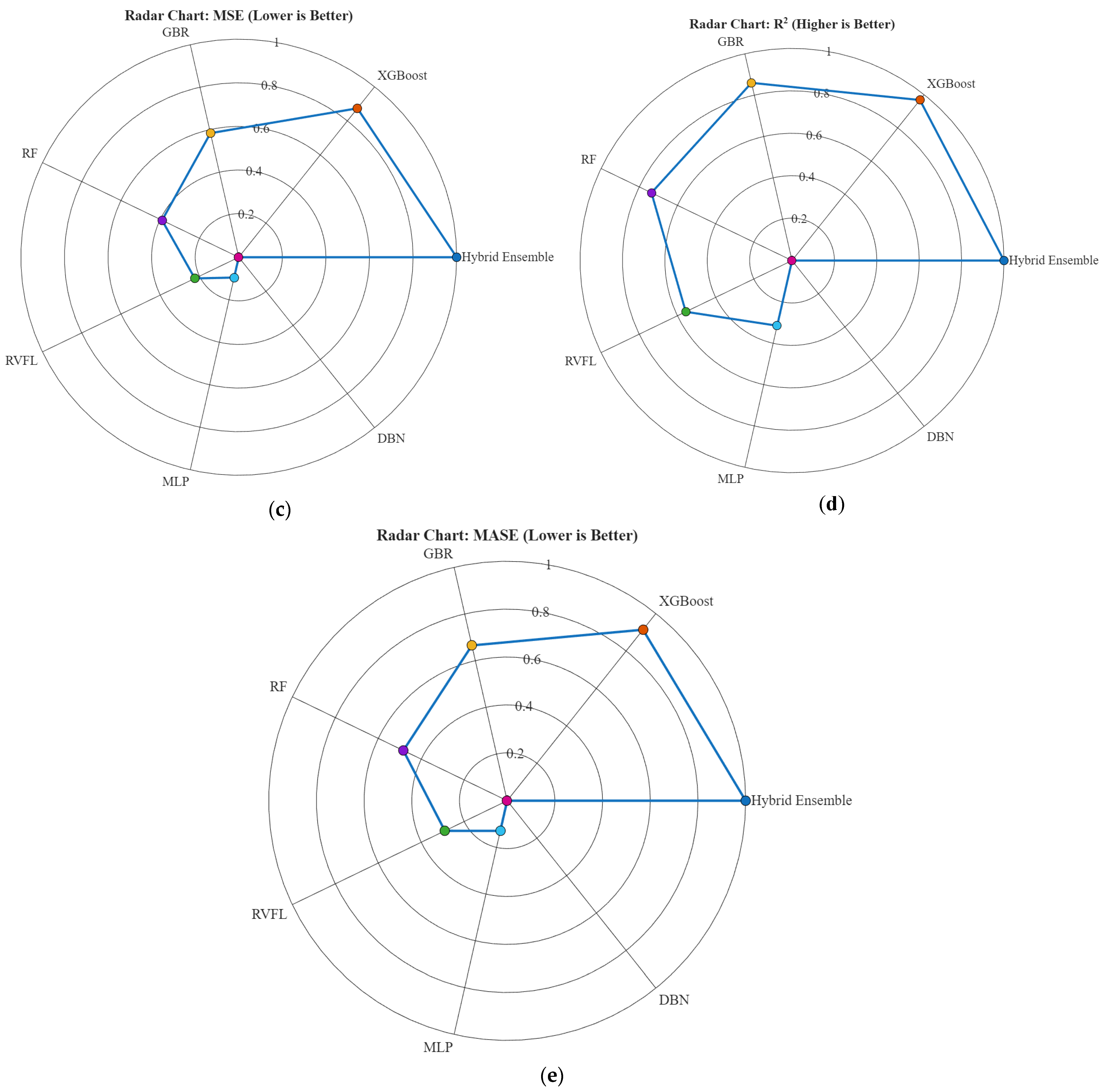
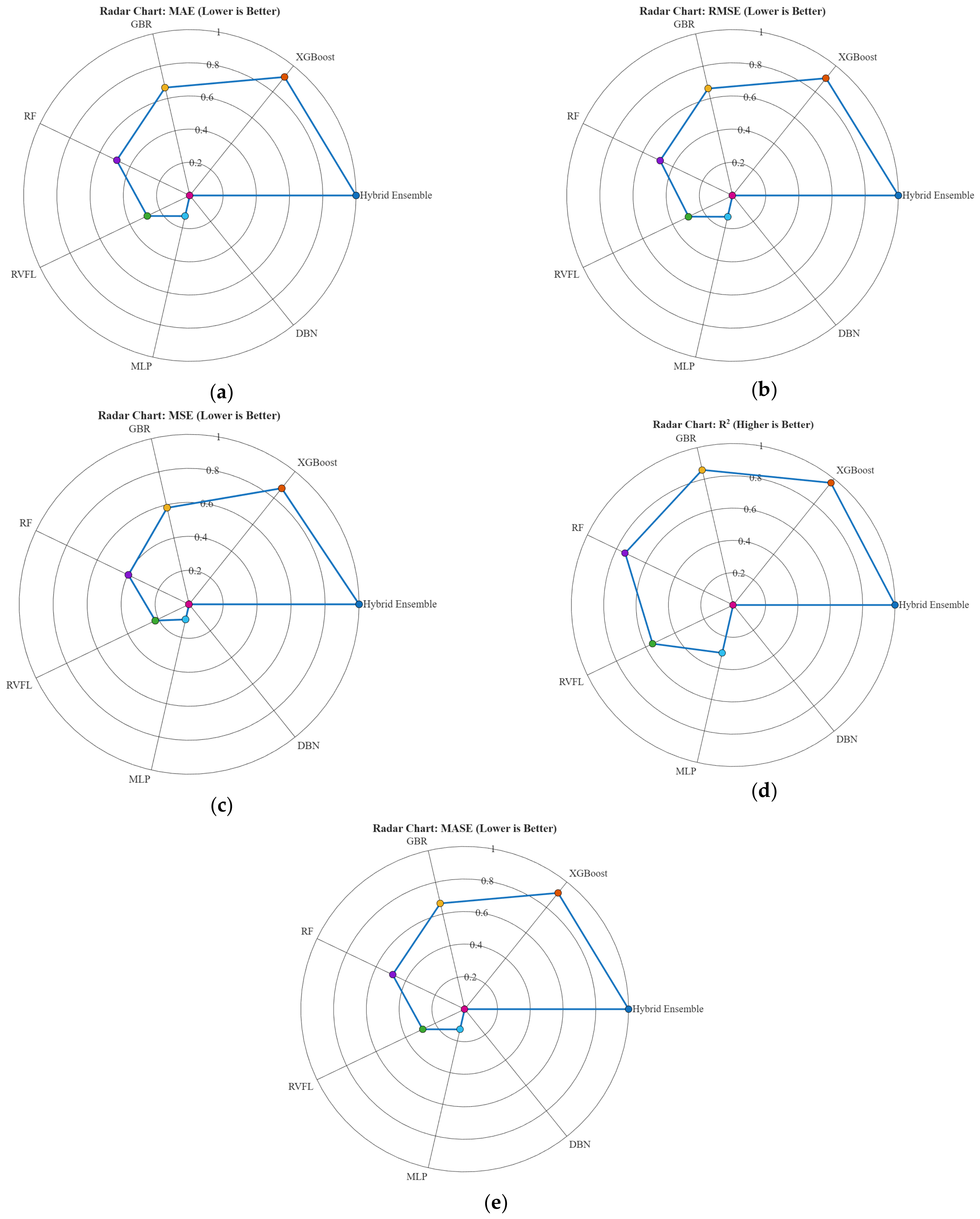
The radar chart presented in Figure 19 shows that the hybrid ensemble model consistently achieved the best performance to confirm its robustness for load demand forecasting. XGBoost and GBR models follow the performance hierarchy by delivering competitive results that are slightly lower than those of the hybrid ensemble model. The DBN and MLP models exhibited limited accuracy and robustness relative to other models used in the study. These results show that the use of hybrid ensemble with multiple learning models can be utilized to improve the predictive performance by modelling the residential energy consumption patterns and variability of load demands. The proposed hybrid ensemble mode can be used for accurate forecasting under variety of load conditions such as smart energy management and demand-side planning applications.

3.2. Solar Irradiance Forecasting

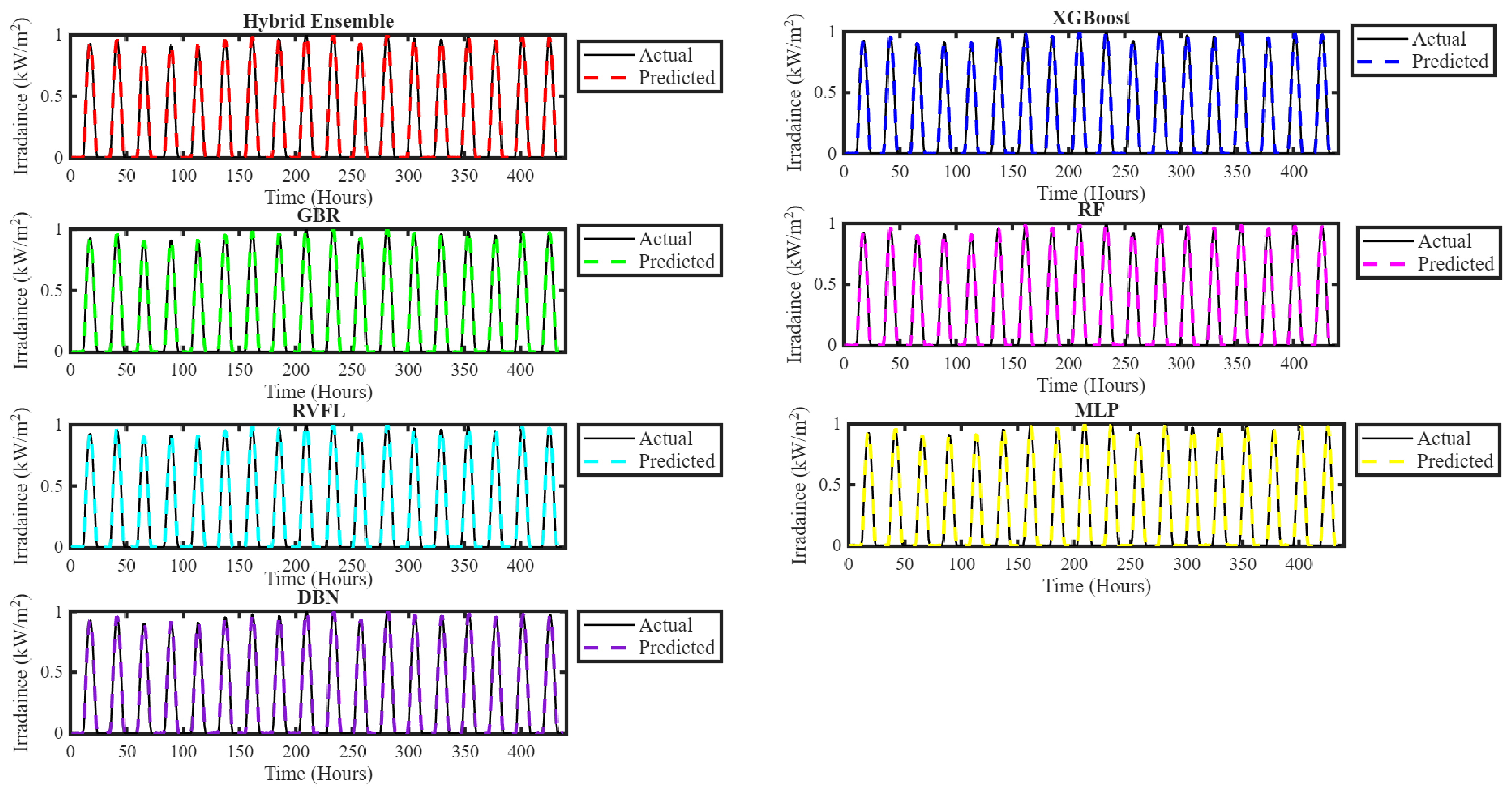
Solar irradiance forecasting is crucial for the optimization of PV energy generation and improvement of energy management in residential systems. The forecasting performance of RF, GBR, XGBoost, DBN, MLP, RVFL and hybrid ensemble models is evaluated in this section as presented in Figure 20. The results show that the hybrid ensemble model provided the closest agreement with the actual irradiance profile, with the predicted values almost overlapped the observed data throughout the forecasting period. This indicates its superior capability in capturing both the nonlinear characteristics and short-term variability of solar irradiance. XGBoost accurately tracked the trend and peak irradiance values with small deviation to show good prediction performance. The performance of GBR is moderately recognized as one of the best with slight variations noted with sudden changes in solar irradiance. The RF and RVFL models also demonstrate moderate performance with a strong capability to capture the overall trend of the irradiance profile. The MLP and DBN models have relatively poor performance with visible deviations from the actual irradiance curve. The superior performance of the hybrid model is based on the significance of using several learning strategies to improve prediction accuracy in extremely unpredictable energy systems.
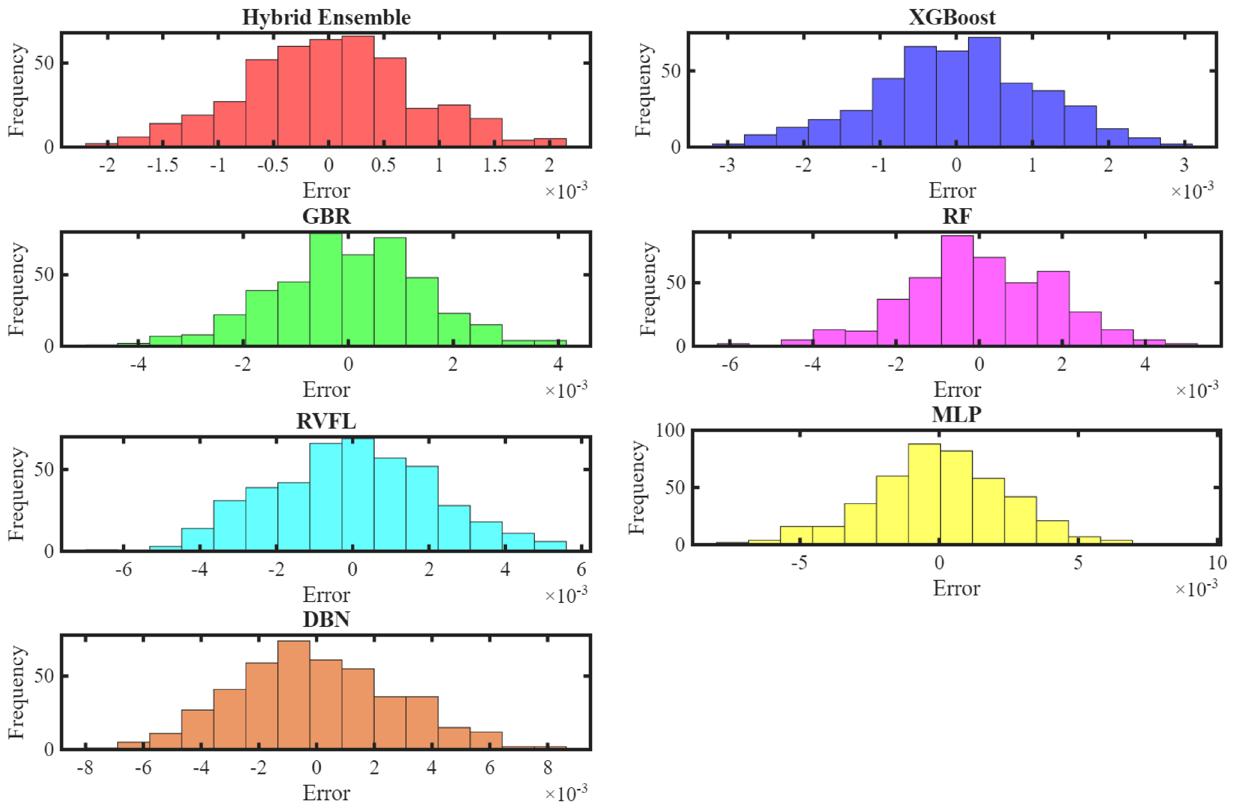
The hourly error distribution (histogram) of solar irradiance forecasting models that consists of RF, GBR, XGBoost, DBN, RVFL, MLP and the hybrid ensemble models. It can be established from the error histograms presented in Figure 21 that there is a considerable difference in the performance of each model. The hybrid model has a highly concentrated error distribution around zero to indicate accurate and consistent predictions with very small deviations between predicted and actual values. The distribution of XGBoost and GBR models are narrow and well centred to demonstrate high prediction accuracy and consistency with the capability of moderate deviation. The wider distributions of RF and RVFL indicate higher uncertainty and less consistent performance. It can be seen in Figure 21 that RF has noticeable spread on both sides while RVFL exhibits even broader dispersion. MLP and DBN models have the widest distributions to indicate the highest prediction uncertainty. This shows that errors are more spread out with visible tails to reflect reduced accuracy and consistency. The histogram analysis established that the robustness of the hybrid model can be used to minimize large deviations, this is crucial for renewable energy system scheduling and grid integration.
The statistical error analysis for solar irradiance prediction across the evaluated models is presented in Table 3. The mean error for all models is extremely close to zero to indicate that all models are effectively unbiased in predicting solar irradiance. Excellent agreement between projected and actual values is reflected in the near-zero bias. The hybrid ensemble has the lowest error range of 0.0042422 and standard deviation error of 0.00078, followed by XGBoost and GBR with error range of 0.006018 and 0.0087583 and standard deviation error of 0.0011167 and 0.0014533. This demonstrates their superior consistency and stability relative to other models. The results presented in Table 3 demonstrate that RF and RVFL models have error range of 0.010948 and 0.11901 and standard deviation error of 0.00179 and 0.0021267. MLP and DBN exhibit the highest variability with error range of 0.016246 and 0.01638 and standard deviation error of 0.0024633 and 0.0028. The results indicate reduced predictive reliability of MLP and DBN models. The skewness values are generally closed to zero to suggest near-symmetric error distributions. Slight negative skewness of −0.12103, −0.16826 and−0.1621 are observed in XGBoost, GBR and RF to suggest a mild tendency toward underestimation. In contrast, hybrid ensemble of 0.03078 and RVFL of 0.029272 are nearly symmetric, while DBN of 0.18222 shows a slight inclination toward overestimation. RF and MLP have slightly higher kurtosis of 3.1443 and 3.3836 to signal the presence of weak outliers and hybrid ensemble and RVFL of 2.8341 and 2.6848 to show more regulated tail behaviour. The results demonstrate that the hybrid ensemble model provides the most accurate and stable solar irradiance predictions, followed by XGBoost and GBR. The performance of MLP and DBN models is not consistent and more variable when compared to other models utilized in the study.
The predictive performance of the solar irradiance forecasting models is assessed using MAE, MSE, RMSE, MASE and R2 as presented in Table 4. The ensemble hybrid produced the lowest MSE of 0.13672, MAE of 0.21969, RMSE of 0.36976 and MASE of 0.0034927 and the highest R2 of 0.98879. The results clearly indicate that the hybrid model outperformed other models in all evaluation metrics. The substantial improvement is attributed to its capability to integrate complementary strengths of many algorithms and improve generalization and robustness. XGBoost demonstrates the best overall performance among the individual models with lower MSE of 0.15149, MAE of 0.23126, RMSE of 0.38922 and MASE of 0.0036765 and the higher R2 of 0.98758. This demonstrates an effective way of capturing the nonlinear relationships present in data on solar irradiance. The GBR model achieved lower MSE of 0.20127, MAE of 0.27229, RMSE of 0.44863 and MASE of 0.0043289 and a higher R2 of 0.9835 compared to RF that has MSE of 0.25769, MAE of 0.313, RMSE of 0.50764, MASE of 0.0049761 and R2 of 0.97887. This indicates that boosting techniques provide better predictive improvement in this application. The RVFL model has a moderate level of predictive accuracy with MSE of 0.34002, MAE of 0.37208, RMSE of 0.58311, MASE of 0.0059154 and R2 of 0.97212. The results demonstrate that the performance of RVFL is better than DBN and MLP but significantly worse than GBR and XGBoost. The MLP model has acceptable performance values with MSE of 0.45069, MAE of 0.44139, RMSE of 0.67134, MASE of 0.0070173 and R2 of 0.96305. The DBN model recorded the weakest performance among the seven models with the highest MSE of 0.59513, MAE of 0.5199, RMSE of 0.77145 and MASE of 0.0082525 and the lowest R2 of 0.95121. The results demonstrate that hybridization of models significantly improved forecasting accuracy by utilizing the strengths of several algorithms. The predictive performance of the hybrid ensemble model is compared with the XGBoost. The comparison show that the hybrid ensemble has superior performance across all evaluation metrics relative to the best standalone model. RMSE reduced from 0.38922 for XGBoost to 0.36976 for the hybrid ensemble, this corresponds to a 5% reduction. Similarly, the MAE and MASE are reduced by 5% to indicate a consistent reduction in forecasting errors. MSE is also reduced by 9.75%, this reduction demonstrates the improved capability of the hybrid model to minimize large prediction deviations. Furthermore, R2 increased from 0.98758 to 0.98879 to confirm the superior predictive performance of the proposed model.
The forecasting performance of each model such as RF, GBR, XGBoost, DBN, MLP, RVFL and hybrid ensemble models is comprehensively visualized in Figure 22. The benefits of hybridizing several models to improve the prediction accuracy of solar irradiance forecasting in smart grid systems are further visualized in the figure. XGBoost model exhibited the second-best performance with a comparatively nearly and fairly symmetrical polygon. It is followed by GBR, RVFL, RF, MLP and DBN models.

3.3. Solar Energy Generation Forecasting

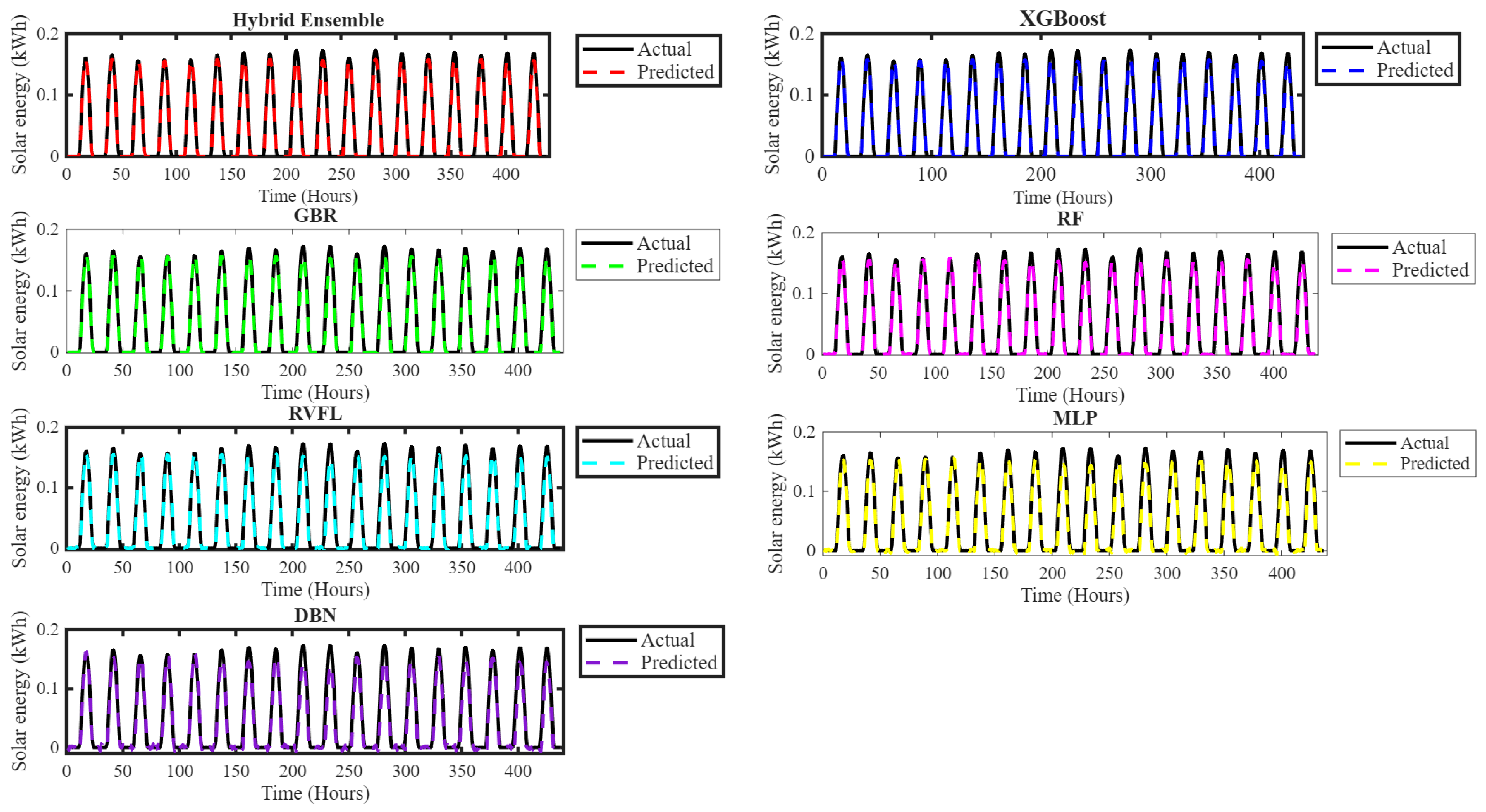
Solar energy generation forecasting is essential for the improvement of PV system operation and energy management in residential systems. The forecasting performance of GBR, RF, DBN, XGBoost, MLP, RVFL and a hybrid ensemble model is evaluated in this section. The results are assessed using standard statistical error metrics that provide an extensive evaluation of model performance under varying operating conditions. The time-series comparison between the actual and predicted solar energy is presented in Figure 23. The hybrid ensemble model has the most accurate predictions with the forecasted values that are closely matched the actual PV output throughout all time intervals. XGBoost has good predictive performance by closely tracking the actual output of the PV system with minimal deviation. The GBR also has good agreement with the observed data with slight deviation from actual solar energy generation. The RF and RVFL models demonstrate moderate performance. They can successfully capture the general pattern of solar energy generation by showing noticeable smoothing of peak values. The MLP and DBN models have the lowest performance with obvious deviations from the actual output of the photovoltaic system. It can be confirmed from the comparative analysis of the results that hybrid and boosting-based approaches are more effective in capturing the complex temporal dynamics of solar energy generation. This makes them highly suitable for real-time forecasting applications in smart grid and renewable energy systems.
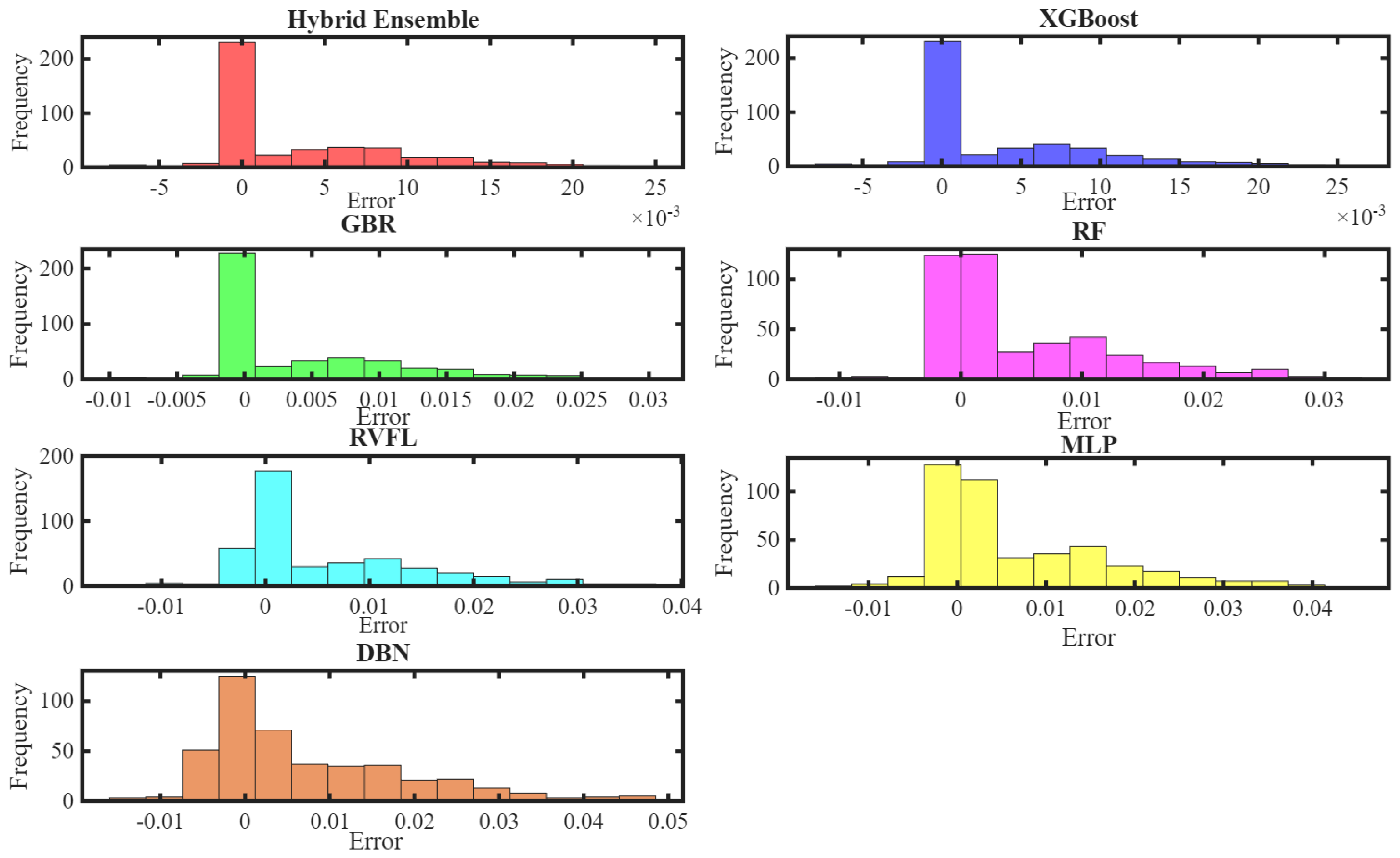
The hourly error distribution of solar energy generation forecasting based on different models is presented in Figure 24. The best performance of the ensemble approach is attributed to a highly concentrated and symmetric error distribution near zero. The hybrid ensemble model is characterized by low variance and strong predictive accuracy that are based on the narrow spread. The XGBoost and GBR models followed closely by revealing a small wider distribution error that reflect strong predictive accuracy. The RF and RVFL models have broader distribution errors with very high deviation. This demonstrates acceptable performance that has continuously reduced when compared to boosting-based approaches. On the other hand, MLP and DBN models have the longest up tails and the biggest error spreads to indicate greatest uncertainty and worst predictive reliability.
The solar energy statistics reflect the final operational efficiency and the capacity of the model to manage the nonlinear conversion factors of the photovoltaic system. The hybrid ensemble model has the best predictive accuracy with the lowest mean error of 0.0036524, closely followed by XGBoost and GBR with mean errors of 0.0038446 and 0.0044503 as presented in Table 5. Conversely, MLP and DBN have relatively higher bias with mean error of 0.0065747 and 0.0073378, demonstrating their reduced accuracy. The mean error progression among models follows the same ranking as shown in Figure 22 to show consistency between visual and numerical analyses. The error dispersion metrics such as error range and standard deviation are used in this section to further highlight the performance disparities. The hybrid ensemble achieved the smallest error range of 0.031556 and standard deviation of 0.0055544 to indicate its highly consistent predictions. XGBoost and GBR followed with error range of 0.033217 and 0.037853 and standard deviation of 0.0058467 and 0.0067349 to demonstrate their slightly higher variability. RF and RVFL show moderate dispersion with error range of 0.04264 and 0.049077 and standard deviation of 0.0075844 and 0.008787. The largest variability is observed in MLP and DBN, with error ranges of 0.060249 and 0.062306 and standard deviations of 0.010193 and 0.011764, confirming their lower stability. These findings indicate that the hybrid model increased accuracy and prediction stability. All models exhibit positive skewness of 1.1135–1.2619 to indicate their right-skewed error distributions with occasional large positive errors. The skewness values progressively reduced from hybrid ensemble to DBN to indicate less asymmetry in lower performing models. The hybrid ensemble and XGBoost have the highest skewness of 1.2619, this demonstrates a clear tendency for sporadic significant positive errors. The hybrid ensemble and XGBoost show slightly higher kurtosis of 4.0197–4.0469 to demonstrate their heavier tails while DBN has a relatively lower kurtosis of 3.8112 with a lower tail intensity.
The performance of solar energy generation forecasting models is assessed in this section using MSE, RMSE, MAE, R2 and MASE. It can be seen from the results presented in Table 6 that the hybrid model continuously performed better than the other models in every evaluation metric. It has the highest R2 of 0.98884 and the lowest MSE of 4.412 × 10⁻¹, MAE of 0.0039487, RMSE of 0.0066423 and MASE of 0.34876. The hybridization of different models and superior ability to accurately capture the intermittent nature of solar energy are responsible for the best performance of the hybrid ensemble approach. In a comparable direction, XGBoost emerged as an effective model among individual models with MSE of 4.8887 × 10⁻¹, MAE of 0.0041566, RMSE of 0.0069919, MASE of 0.36712 and R2 of 0.98763. The excellent performance of XGBoost has been attributed to its ability to describe the intricate nonlinear relationships and temporal dependencies present in solar energy generation data. The GBR model demonstrated competitive performance with MSE of 6.5061 × 10⁻², MAE of 0.0048926, RMSE of 0.008066, MASE of 0.43212, and R2 of 0.98354. It has relatively low error values to confirm the effectiveness of the GBR model in forecasting of solar energy generation. The RF model has a lower R2 of 0.97915 and a significantly higher MSE of 8.2399 × 10⁻¹, MAE of 0.0056119, RMSE of 0.0090774 and MASE of 0.49565. This indicates limitations in modelling complex patterns despite its robustness. The RVFL model has moderate predictive ability with MSE of 0.00011032, MAE of 0.0067404, RMSE of 0.010503, MASE of 0.59533 and R2 of 0.97209. It has an inferior performance when compared to boosting-based models. The MLP model has higher MSE of 0.00014688, MAE of 0.0079814, RMSE of 0.01212, MASE of 0.70494 and lower R2 of 0.932 to demonstrate acceptable performance but with relatively higher prediction errors. The DBN recorded the poorest performance among all models with the highest MSE of 0.00019191, MAE of 0.0093814, RMSE of 0.013853 and MASE of 0.82859 and the lowest R2 of 0.95144. This implies that the DBN model is not effective for the specified dataset owing to inadequate training data. The outcomes of the study clearly show that ensemble hybrid, XGBoost and GBR approaches are significantly better than RF, RVFL, MLP and DBN models in solar energy generation forecasting. The performance of the hybrid model is assessed in this section by comparing its metrics with the best standalone model (XGBoost). It can be seen from the outcomes of the study that RMSE of the hybrid model reduced from 0.0069919 to 0.0066423, this demonstrates a 5.00% reduction. Similarly, the values of MAE and MASE reduced by 5.00% to indicate a reduction in forecasting errors. In addition, the MSE reduced by 9.75%, this reveals a minimum prediction deviation. R2 increased from 0.98763 to 0.98884, this indicates an improved ability of the hybrid model to capture the variability of solar energy generation.
A radar chart is a multi-dimensional comparative visualization that can be used to evaluate the forecasting performance of solar energy using statistical error metrics. The numerical values shown in Table 6 are visually confirmed by the radar chart presented in Figure 25. The figure clearly shows that the hybrid ensemble model is better than all the other forecasting models in terms of the selected performance indicators. XGBoost and GBR models are ranked second and third based on their high predictive accuracy and robustness, but their performance is slightly inferior to the hybrid ensemble model. The RF and RVFL models attained moderate performance, while the MLP and DBN models produced comparatively lower forecasting accuracy and consistency. This analysis shows that hybrid and boosting-based models can be used in the power system to improve the performance of solar energy generation forecasting.

3.4. Electricity Bill Forecasting

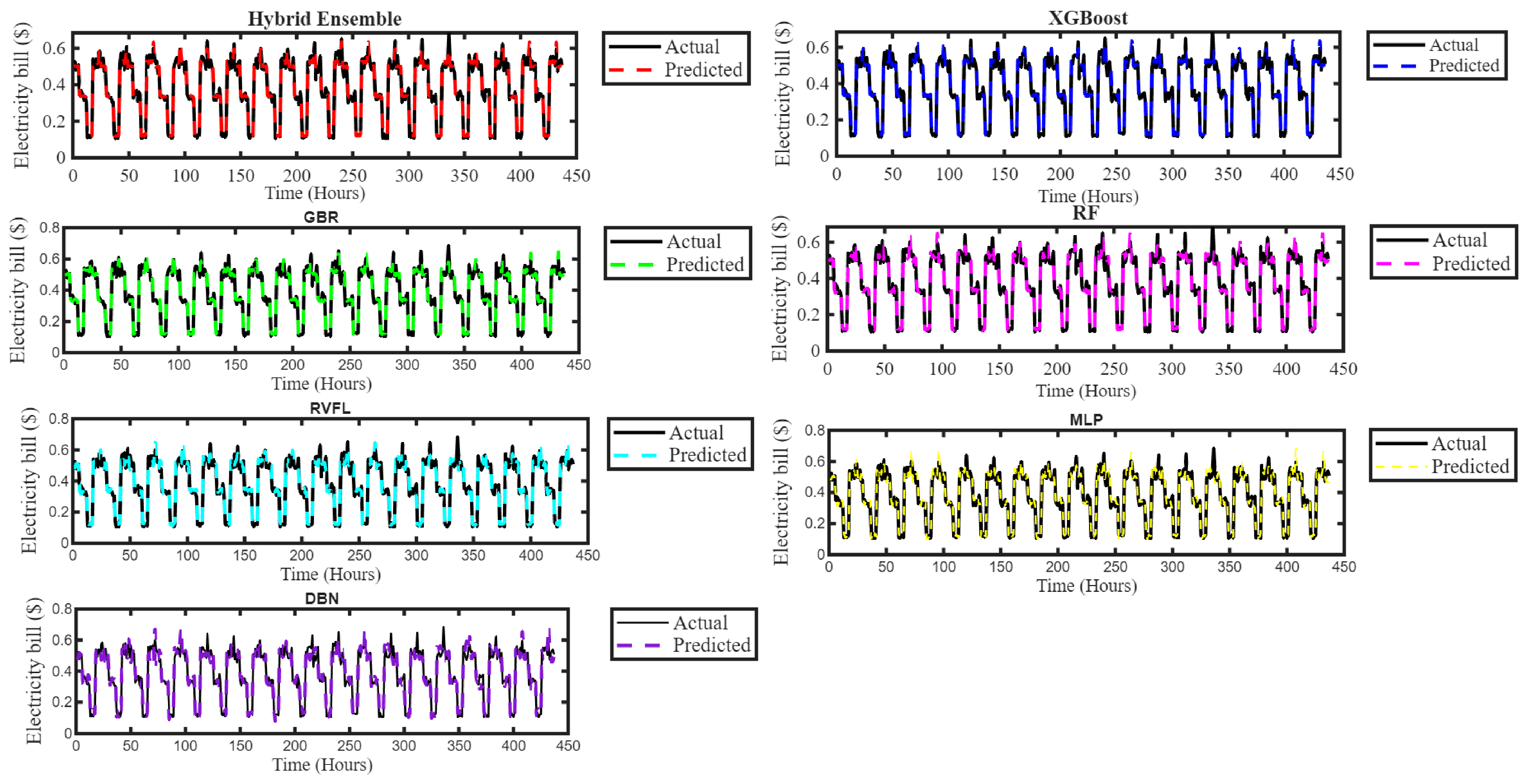
Electricity bill forecasting is a significant component of residential building energy system where prices of electricity fluctuate throughout the day. Customers can optimize energy consumption, schedule household appliances and reduce expenses when electricity bills are accurately predicted. RF, GBR, XGBoost, DBN, MLP, RVFL and hybrid ensemble models are utilized in this section to forecast electricity bills. The time-series comparison between the actual and predicted electricity bills for RF, GBR, XGBoost, DBN, RVFL, MLP and hybrid ensemble models over an extended forecasting horizon of approximately 450 h is presented in Figure 26. The hybrid model has the best agreement with the actual electricity bill profile and the projected values almost overlapped the observed data throughout the time horizon. XGBoost has a very strong prediction performance that closely tracked the real billing trend. Similarly, GBR has a very good agreement with the actual values but with some smoothing and latency during peak cost periods. The main trend and periodicity of the electricity bill are captured by RF but peak values are smoothed out, and high-cost periods are slightly underestimated. This indicates limited responsiveness to sharp variations in tariff and demand. RVFL demonstrates moderate performance in tracking the general pattern effectively but shows noticeable deviations during peak and transition periods. DBN shows the poorest performance that is characterized by significant deviations from actual values, irregular prediction patterns and poor tracking of periodic billing behaviour.
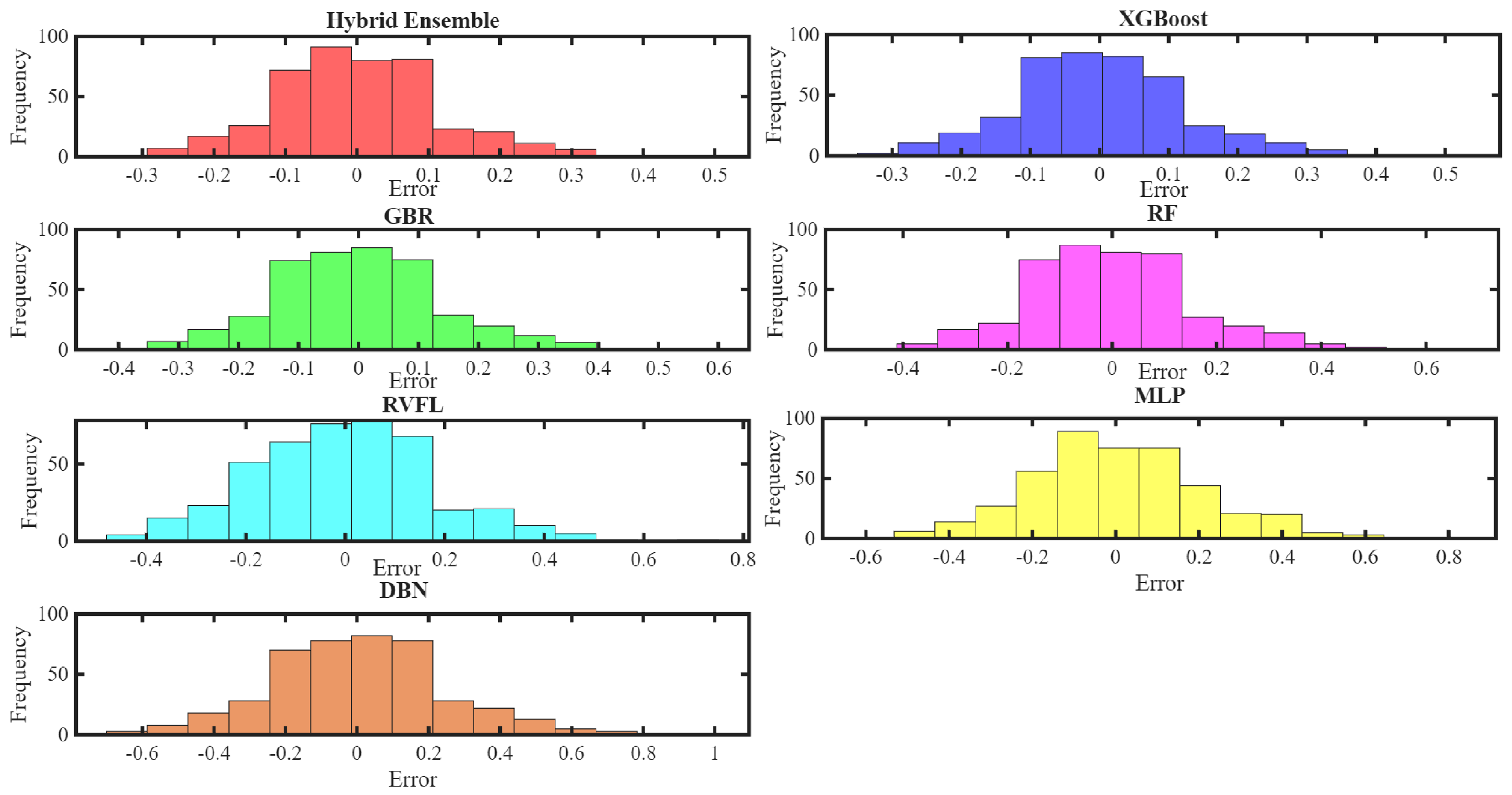
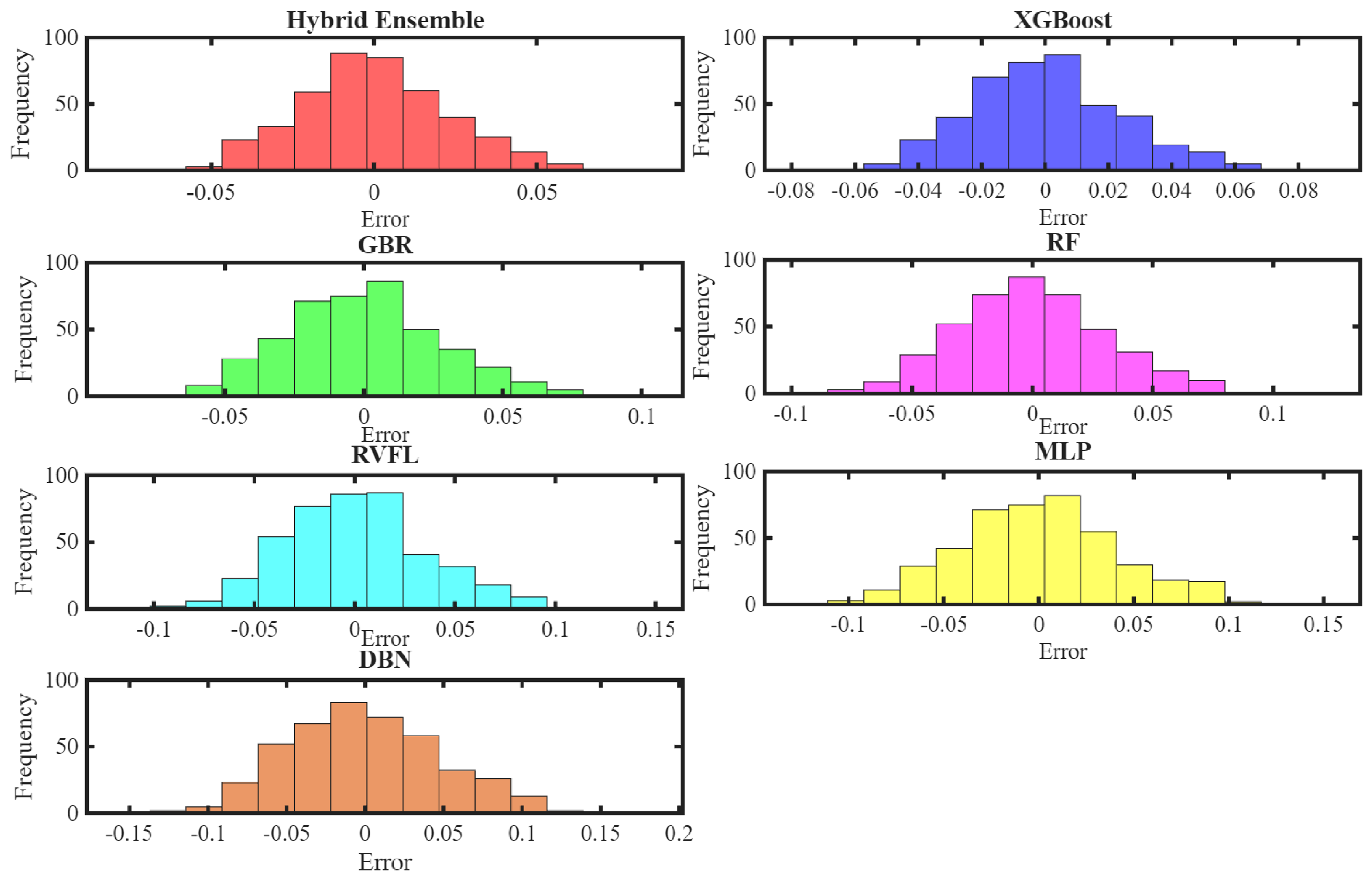
The analysis of the error distribution histograms for electricity bill forecasting and the corresponding statistical error metrics to provide an in-depth assessment of models’ accuracy, variability and distributional behaviours. The hybrid ensemble model exhibits the most concentrated and symmetric distribution around zero to indicate high prediction accuracy, low variance and minimal bias as shown in Figure 27. The narrow spread of the hybrid ensemble can be used to validate its ability to consistently predict electricity costs under various conditions. Additionally, XGBoost and GBR show comparatively narrow error distributions with a moderate dispersion and the majority of errors concentrated close to zero. RF and RVFL models have wider spreads and longer tails to indicate greater variability, less bias and less consistent predictions when compared to boosting models. The MLP and DBN models have the widest spread distributions with substantial deviation and heavy tails to indicate high prediction errors and volatility in the modelling of cost dynamics.
The statistical error metrics for electricity bill prediction such as mean error, range, standard deviation, skewness and kurtosis are presented in this section. The results shown in Table 7 demonstrate that the mean error values are generally closed to zero, which indicates minimal bias across all models. The hybrid ensemble and XGBoost demonstrate low bias with the values of mean error of 0.00030015 and 0.00031595. While RVFL recorded the smallest mean error of 9.8036 × 10⁻⁵ to suggest near-unbiased predictions. This does not translate into better performance due to its significantly larger variability. DBN shows the highest mean error of 0.00091745 to indicate its relatively reduced accuracy. The hybrid ensemble has the smallest range and standard deviation of 0.15567 and 0.022985. This shows that the model has the most stable and consistent prediction in terms of error dispersion. XGBoost and GBR followed closely with error range of 0.16386 and 0.18931 and standard deviation of 0.024195 and 0.027853. While RF and RVFL show moderate variability with error range of 0.2133 and 0.2397 and standard deviation of 0.031483 and 0.036605. The highest dispersion is observed in MLP and DBN with error range of 0.29598 and 0.313846 and standard deviation of 0.042034 and 0.04974. Skewness values for all models are positive from range of 0.12609 to 0.27315 to indicate slightly right-skewed error distributions and occasional underestimation. The values remain relatively small with near-symmetric distributions. MLP exhibits a higher kurtosis of 3.3839 to indicate heavier tails and a greater likelihood of extreme errors. The hybrid ensemble has a kurtosis of 3.1317 to maintain near-normal behaviours and balanced distribution with limited outliers. DBN also showed a high kurtosis of 3.1588 that is consistent with its wide error spread. These results demonstrate the effectiveness of an ensemble model for accurate electricity bill forecasting.
The performance of the electricity bill forecasting models is evaluated in this section using statistical metrics presented in Section 2.4. The performance of each model for the assessment period is presented in Table 8. It can be seen from the results that the hybrid ensemble model achieved the best performance with the lowest MSE of 0.00052719, MAE of 0.018126, RMSE of 0.022961 and MASE of 0.30006 and the highest R2 of 0.97978. This shows excellent predicting performance of the hybrid ensemble model with a significant correlation with observed values and minimal variation from actual electricity bills. XGBoost achieved relatively low MSE of 0.00058414, MAE of 0.01908, RMSE of 0.024169 and MASE of 0.31585 and high R2 of 0.97759 to indicate its competitive performance. The GBR also demonstrates strong predictive capability to achieve MSE of 0.00077666, MAE of 0.022002, RMSE of 0.027869 and MASE of 0.36421 and R2 of 0.97021. These results can be used to reinforce the suitability of boosting-based ensemble approaches for energy forecasting applications. The RF model yields comparatively higher MSE of 0.000994, MAE of 0.024906, RMSE of 0.029080, MASE of 0.4123 and R2 of 0.96187. This demonstrates that the RF model is less effective in capturing intricate nonlinear dependencies in solar energy generation data when compared with boosting-based approaches. The RVFL model shows moderate performance with MSE of 0.0012985, MAE of 0.028561, RMSE of 0.036035, MASE of 0.4728 and R2 of 0.95019 to provide a reasonable balance between prediction accuracy and computational efficiency. However, its performance remains inferior to that of the boosting-based models. The MLP model demonstrates acceptable performance with MSE of 0.0017742, MAE of 0.033358, RMSE of 0.042121, MASE of 0.5522 and R2 of 0.93194. The performance of the DBN is the poorest among the assessed models with the highest MSE of 0.0023968, MAE of 0.039109, RMSE of 0.048957, MASE of 0.64741 and the lowest R2 of 0.90806. The effectiveness of the hybrid ensemble model has been revealed in the study through the comparison of XGBoost and hybrid ensemble models. The findings showed that the reduction in RMSE is achieved from 0.024169 to 0.022961 with improvement of 5.00%; whereas, MAE and MASE are reduced by 5.00%. In addition, MSE is reduced by 9.75%, while the value of R2 increased from 0.97759 to 0.97978.
It can be established from the results presented in Table 8 that hybrid and boosting-based models considerably improved forecasting accuracy and reliability for electricity bill. These models can be deployed in smart grid operations, renewable energy integration system and advanced energy management systems where accurate and reliable electricity bill forecasting is essential for making the best decisions.
The radar chart comparison of the electricity bill forecasting models, including RF, GBR, XGBoost, MLP, DBN, RVFL and the hybrid ensemble model is presented in Figure 28. The radar chart efficiently illustrates the relative capabilities of each model. It is obvious from the figure the radar chart that the hybrid ensemble model consistently occupied the outermost region to demonstrate its superior forecasting performance. This is achieved by its lowest values of MAE, MSE, MASE and RMSE, coupled with the highest value of R2 when compared to other evaluated forecasting models. The XGBoost and GBR models ranked second and third in terms of forecasting performance relative to hybrid ensemble model. The RF, RVFL, MLP and DBN show relatively poor performance across the selected evaluation metrics when compared to hybrid ensemble model. This indicates that hybrid ensemble approach can provide strong and balanced performance across all metrics.

3.5. Comparative Analysis of Forecasting Models

The radar chart presented in Figure 29a–d reveals that the hybrid ensemble model consistently occupied the outermost area to indicate superior performance in all metrics across all domains. The solid lines indicate superior predictive performance with the lowest error values such as MAE, MSE, MASE and RMSE and the highest R2. This shows that the model can reliably capture both linear trends and nonlinear fluctuations irrespective of the standardized domain. XGBoost and GBR models followed closely with high performance while RF and RVFL models showed poorer performance. RF and RVFL exhibited lower radar chart coverage to indicate relatively poorer predictive accuracy. MLP and DBN models showed poor predicting performance with marginal larger errors. The results presented in this section underscore the robustness and suitability of the hybrid model for practical energy system forecasting applications such as load management, renewable energy integration and electricity cost optimization.
It can be seen from the outcomes of the study that the proposed hybrid ensemble model consistently achieved superior performance compared with the individual forecasting models. The improvement of hybrid ensemble model achieved in this study has been attributed to its ability to combine the complementary strengths of RF, GBR, XGBoost, DBN, RVFL and MLP models. The hybrid model reduced individual model biases and minimized prediction uncertainties by combining the predictions of multiple learners through a validation-based weighting mechanism. The results are interpreted in terms of their practical significance beyond statistical performance. The findings of the study demonstrate that the hybrid model has achieved improved forecasting accuracy which can be used for effective utilization of solar energy generation, reliable estimation of electricity costs under TOU tariffs and improved residential energy management. The results obtained from the study indicate that accurate predictions can lead to improved system efficiency and reduction in electricity bills. Accurate predictions of load demand and solar energy generation can be utilized in energy scheduling, management of battery storage system and demand-side response strategies. The performance of the model in different households, seasons and cities cannot be conclusively established from the current dataset. The proposed hybrid model is effective for short-term forecasting under high-resolution residential data and its applications in several buildings and seasonal conditions will require retraining or domain adaptation. Consequently, additional validation using multi-season, multi-household and geographically diverse datasets is required to fully assess the generalization capability and transferability of the proposed framework.

4. Conclusions

The comprehensive assessment of seven forecasting models such as RF, GBR, XGBoost, MLP, DBN, RVFL and hybrid ensemble models was applied to load demand, solar irradiance, solar energy generation and electricity bill forecasting of a residential building in Durban, South Africa. The performance of each model was evaluated using MAE, MSE, MASE, RMSE and R2. The results indicate that the hybrid ensemble model consistently outperformed all individual models across all metrics and domains and achieved the electricity forecasting bill with the lowest MAE, RMSE, MSE, MASE of 0.018126, 0.022961, 0.00052719 and 0.30006 and the highest R2 of 0.97978 when compared to other models. This demonstrates its exceptional capacity to reduce prediction errors and integrate complementary strengths of several algorithms. The hybrid model showed superior performance in accurate tracking of demand fluctuations with minimized error metrics and improved electricity billing accuracy that supports demand-side energy management. It can be established from the outcomes of the study that hybrid ensemble models are highly suitable for practical applications in smart grids, electricity cost optimization and renewable energy systems based on its robustness and accurate predictions. The future studies must be focused on the hybridization of real-time models with the integration of IoT-enabled energy systems that are capable of further improving forecasting performance and applicability. The proposed hybrid framework demonstrates strong forecasting capability and provides a promising foundation for residential energy forecasting with several limitations such as limited interpretability, increased computational complexity, potential risk of over lifting and limited climatic diversity. The future work should be directed toward improving interpretability, reducing computational complexity and validating performance across multiple households with diverse consumption characteristics and seasonal conditions. This can be achieved by broader deployment of artificial intelligence techniques in smart residential energy management systems. Additional investigations that include external validation, uncertainty analysis and model interpretability techniques are also recommended to further assess the practical applications of the proposed approach.


Author Contributions

Conceptualization, T.A., G.S., P.N.B. and R.K.; Methodology, T.A.; Software, T.A.; Validation, T.A.; Formal analysis, T.A.; Investigation, T.A.; Writing—original draft, T.A.; Writing—review & editing, T.A., G.S., P.N.B. and R.K.; Supervision, G.S. and P.N.B. All authors have read and agreed to the published version of the manuscript.

Funding

This research received no external funding.

Data Availability Statement

The original contributions presented in the study are included in the article; further inquiries can be directed to the author.

Conflicts of Interest

The authors declare no conflicts of interest.

Abbreviations

The following abbreviations are used in this manuscript:
DBNDeep Belief Networks
DLDeep Learning
GBRGradient Boosting Regression
MAEMean Absolute Error
MASEMean Absolute Scaled Error
MSEMean Squared Error
MLMachine Learning
MLPMulti-Layer Perceptron
R2Coefficient of Determination
RFRandom Forest
RMSERoot Mean Square Error
RVFLRandom Vector Functional Link
TOUTime-of-Use
XGBoostExtreme Gradient Boosting

Appendix A

y R F p = 1 T t = 1 T f x ( x )
where T is the number of decision trees, f x ( x ) is the prediction from tree t and y t p is the final predicted value.
F m ( x ) = F m 1 ( x ) + γ m h m ( x )
where F m ( x ) is the updated model, F m 1 ( x ) is the previous model, h m ( x ) is the new decision tree (weak learner) and γ m is the learning rate controlling the contribution of the new tree.
y X G B o o s t p = ϕ ( x i ) = k = 1 K f k ( x i ) , f k F Ψ
where ϕ ( x i ) is the overall model function, y i p is the predicted value for sample i, K is the number of trees, f k is the regression tree and F Ψ is the functional space of trees.
y D B N p = f o u t ( W ( L ) h ( L 1 ) + b ( L )
where W is the weight matrices, L is the number of layers, f o u t is the activation function and b is the bias term.
f o u t x = m a x ( 0 , x )
y R V F L p = h ( x ) β h + x β x
where h ( x ) is the random hidden layer output and β h , β x   = output weights learned via least squares.
h ( x ) = f a c t W r x + b r
where f a c t is the activation function and W r is the output weights.
y M L P p = f o u t ( W ( L ) h ( L 1 ) + b ( L )
where W is the weight matrices, L is the number of layers, f o u t is the activation function and b is the bias term.
y h y b r i d p = 1 n i = 1 n y i p
where y h y b r i d p the final hybrid ensemble prediction, y i p is the prediction from the i t h model and n is the number of models.
y ^ = i = 1 M w i y ^ i
where M is the number of base learners such as RF, GBR, XGBoost, DBN, RVFL and MLP, y ^ i is the prediction of the ith model and w i is the normalized weight assigned to the ith base model in the ensemble.
i = 1 M w i = 1
E i = α 1 R M S E i + α 2 M A E i + α 3 M S E i + α 4 M A S E i
where α 1 , α 2 , α 3 and α 4 are normalization weights.
E i * = E i R i 2 +
where is a small constant to avoid division by zero.
1 E i * j = 1 M 1 E j *
where E j * is the adjusted validation error of the jth model in the ensemble.
M A E = 1 n i = 1 n y i y i p
where y i is the actual value, y i p is the predicted value and n is the number of observations.
R M S E = 1 n i = 1 n y i y i p 2
R 2 = 1 i = 1 n y i y i p 2 i = 1 n y i y i m 2
where y i m is the mean of observed values.
M S E = 1 n i = 1 n y i y i p 2
M A S E = 1 n i = 1 n y i y i p 1 n 1 i = 2 n y i y i p 1
e i = y i y i p
where e i is the error associated with the ith observation.
μ e = 1 n i = 1 n e i
σ e = 1 n i = 1 n e i μ e 2
R a n g e = min ( e i ) , max ( e i )
where min ( e i ) and max ( e i ) are the minimum and maximum errors associated with the ith observation.
δ s = 1 n i = 1 n e i μ e σ e 3
ψ k = 1 n i = 1 n e i μ e σ e 4

References

  1. Choudhary, A.K. Environmental Aspects and Electrical Energy Generation. In Renewable Energy Development: Technology, Material and Sustainability; Springer: Singapore, 2025; pp. 327–350. [Google Scholar] [CrossRef] [Scilit]
  2. Adefarati, T.; Potgieter, S.; Sharma, G.; Bansal, R.C.; Onaolapo, A.K.; Borisade, S.G.; Oloye, A.O. Optimization of renewable energy based hybrid energy system using evolutionary computational techniques. Smart Grids Sustain. Energy 2025, 10, 15. [Google Scholar] [CrossRef] [Scilit]
  3. Adefarati, T.; Bansal, R.; Naidoo, R.; Onaolapo, K.; Bettayeb, M.; Olulope, P.; Sobowale, A. Design and techno-economic assessment of a standalone photovoltaic-diesel-battery hybrid energy system for electrification of rural areas: A step towards sustainable development. Renew. Energy 2024, 227, 120556. [Google Scholar] [CrossRef] [Scilit]
  4. Adefarati, T.; Sharma, G.; Bokoro, P.N.; Kumar, R. Advancing renewable-dominant power systems through internet of things and artificial intelligence: A comprehensive review. Energies 2025, 18, 5243. [Google Scholar] [CrossRef] [Scilit]
  5. Adefarati, T.; Sharma, G.; Bokoro, P.N.; Kumar, R. Optimal Scheduling Strategies for Smart Homes Integrated with Grid-Connected Hybrid Renewable Energy Systems. Energies 2026, 19, 1174. [Google Scholar] [CrossRef] [Scilit]
  6. Kumawat, M.; Onaolapo, A.; Sharma, G.; Barutcu, I.C.; Adefarati, T.; Bansal, R. Integrated encoder-decoder-based wide and deep convolution neural networks strategy for electricity theft arbitration. J. Eng. Appl. Sci. 2024, 71, 94. [Google Scholar] [CrossRef] [Scilit]
  7. Eltohamy, M.S.; Aldawsari, M.S.M.; Sadek, A.R.A.; Hegazy, H.Y.A.-H.; Ahmed, I.; Alsenani, T.R.; Kim, Y.-S.; Ahmed, M.M.R. Enhancing Electric Grid Flexibility for the Integration of Variable Renewable Energy: Challenges, Innovations, and Future Directions. IEEE Access 2026, 14, 23080–23109. [Google Scholar] [CrossRef] [Scilit]
  8. Panda, S.K. Electrical load and solar power forecasting using machine learning techniques. J. King Saud Univ. Eng. Sci. 2025, 37, 11. [Google Scholar] [CrossRef] [Scilit]
  9. Han, Y.; Lam, J.C.K.; Li, V.O.K.; Newbery, D.; Guo, P.; Chan, K. A deep learning approach for fairness-based time of use tariff design. Energy Policy 2024, 192, 114230. [Google Scholar] [CrossRef] [Scilit]
  10. Malakouti, M. Machine learning for renewable energy forecasting: Advances, challenges, and future directions. Sustain. Energy Res. 2026, 13, 14. [Google Scholar] [CrossRef] [Scilit]
  11. Hossain, M.; Shams, S.; Ullah, S. Time-series and deep learning approaches for renewable energy forecasting in Dhaka: A comparative study of ARIMA, SARIMA, and LSTM models. Discov. Sustain. 2025, 6, 775. [Google Scholar] [CrossRef] [Scilit]
  12. Houssein, E.H.; Mohamed, M.; Younis, E.M.; Mohamed, W.M. Artificial intelligence and classical statistical models for time series forecasting: A comprehensive review. J. Big Data 2025, 12, 271. [Google Scholar] [CrossRef] [Scilit]
  13. Liu, Y.; Du, Y. A deep Learning–Random forest hybrid model for predicting historical temperature variations driven by air pollution: Methodological insights from wuhan. Atmosphere 2025, 16, 1056. [Google Scholar] [CrossRef] [Scilit]
  14. Hu, Z.; Gao, Y.; Ji, S.; Mae, M.; Imaizumi, T. Improved multistep ahead photovoltaic power prediction model based on LSTM and self-attention with weather forecast data. Appl. Energy 2024, 359, 122709. [Google Scholar] [CrossRef] [Scilit]
  15. Jayathilaka, N.; Warnasooriya, D.J.S.; Nagarajah, K.; Mukunthan, T.; Jalini, S.; Logeeshan, V.; Wanigasekara, C. Deep learning-based regional electricity demand prediction using smart meter data in Sri Lanka. IEEE Access 2026, 14, 50127–50140. [Google Scholar] [CrossRef] [Scilit]
  16. ElNaggar, K.; Amer, R.M.M.; El-Zonkoly, A. Toward grid-interactive and low-carbon buildings: A comparative analysis of artificial intelligence-driven optimization of renewable sizing and demand-side control. Int. J. Optim. Control Theor. Appl. 2026, 16, 025460200. [Google Scholar] [CrossRef] [Scilit]
  17. Vaish, J.; Tiwari, A.K. Empirical mode decomposition with random forest model based short term load forecasting. Distrib. Gener. Altern. Energy J. 2022, 37, 1159–1190. [Google Scholar] [CrossRef] [Scilit]
  18. Mosetlhe, T.; Yusuff, A.A. Forecasting of residential energy utilisation based on regression machine learning schemes. Energies 2024, 17, 4681. [Google Scholar] [CrossRef] [Scilit]
  19. Parizad, B.; Ranjbarzadeh, H.; Jamali, A.; Khayyam, H. An intelligent hybrid machine learning model for sustainable forecasting of home energy demand and electricity price. Sustainability 2024, 16, 2328. [Google Scholar] [CrossRef] [Scilit]
  20. Saini, P.; Parida, S.K. A novel probabilistic gradient boosting model with multi-approach feature selection and iterative seasonal trend decomposition for short-term load forecasting. Energy 2024, 294, 130975. [Google Scholar] [CrossRef] [Scilit]
  21. Cui, J.; Kuang, W.; Geng, K.; Bi, A.; Bi, F.; Zheng, X.; Lin, C. Advanced short-term load forecasting with XGBoost-RF feature selection and CNN-GRU. Processes 2024, 12, 2466. [Google Scholar] [CrossRef] [Scilit]
  22. Yu, H.; Sun, H.; Li, Y.; Xu, C.; Du, C. Enhanced short-term load forecasting: Error-weighted and hybrid model approach. Energies 2024, 17, 5304. [Google Scholar] [CrossRef] [Scilit]
  23. Han, P.; He, W.; Cao, Y.; Li, Y.; Zhang, Y. Deep belief rule based photovoltaic power forecasting method with interpretability. Sci. Rep. 2022, 12, 14467. [Google Scholar] [CrossRef] [Scilit] [PubMed]
  24. Wu, J.; Tang, X.; Zhou, D.; Deng, W.; Cai, Q. Application of improved DBN and GRU based on intelligent optimization algorithm in power load identification and prediction. Energy Inform. 2024, 7, 36. [Google Scholar] [CrossRef] [Scilit]
  25. Shin, S.M.; Rasheed, A.; Kil-Heum, P.; Veluvolu, K.C. Fast and accurate short-term load forecasting with a hybrid model. Electronics 2024, 13, 1079. [Google Scholar] [CrossRef] [Scilit]
  26. Shi, Q.; Katuwal, R.; Suganthan, P.N.; Tanveer, M. Random vector functional link neural network based ensemble deep learning. Pattern Recognit. 2021, 117, 107978. [Google Scholar] [CrossRef] [Scilit]
  27. Peplinski, M.; Dilkina, B.; Chen, M.; Silva, S.J.; Ban-Weiss, G.A.; Sanders, K.A. A machine learning framework to estimate residential electricity demand based on smart meter electricity, climate, building characteristics, and socioeconomic datasets. Appl. Energy 2023, 357, 122413. [Google Scholar] [CrossRef] [Scilit]
  28. Zhou, L.; Zhou, Y.; Liu, L.; Zhao, X. A comparative study of different deep learning methods for time-series probabilistic residential load power forecasting. Front. Energy Res. 2024, 12, 1490152. [Google Scholar] [CrossRef] [Scilit]
  29. Banik, R.; Biswas, A. Enhanced renewable power and load forecasting using RF-XGBoost stacked ensemble. Electr. Eng. 2024, 106, 4947–4967. [Google Scholar] [CrossRef] [Scilit]
  30. Muqtadir, A.; Li, B.; Ying, Z.; Songsong, C.; Kazmi, S.N. Nowcasting the next hour of residential load using boosting ensemble machines. Sci. Rep. 2025, 15, 7157. [Google Scholar] [CrossRef] [Scilit] [PubMed]
  31. Simaiya, S.; Dahiya, M.; Tomar, S.; Faujdar, N.; Sharma, Y.K.; Nuristani, N. A transfer learning-based hybrid model with LightGBM for smart grid short-term energy load prediction. Energy Explor. Exploit. 2024, 42, 1853–1876. [Google Scholar] [CrossRef] [Scilit]
  32. Chen, H.; Huang, H.; Zheng, Y.; Yang, B. A load forecasting approach for integrated energy systems based on aggregation hybrid modal decomposition and combined model. Appl. Energy 2024, 375, 124166. [Google Scholar] [CrossRef] [Scilit]
  33. Haggag, M.; Abdelhady, K.; Guirguis, M.; Saudy, M.; Dakhakhni, W.E. Machine learning long-term electricity demand forecasting system for strategic energy investments. Sci. Rep. 2026, 16, 12471. [Google Scholar] [CrossRef] [Scilit] [PubMed]
  34. Cordon, D.; Pita, A.; Juan, A.A. Classifying and predicting household energy consumption using data analytics and machine learning. Algorithms 2026, 19, 114. [Google Scholar] [CrossRef] [Scilit]
  35. Asiri, M.M.; Aldehim, G.; Alotaibi, F.A.; Alnfiai, M.M.; Assiri, M.; Mahmud, A. Short-term load forecasting in smart grids using hybrid deep learning. IEEE Access 2024, 12, 23504–23513. [Google Scholar] [CrossRef] [Scilit]
  36. Azad, A.S.; Fahd, A.B.; Adhikary, A. Data Preprocessing for Feature Synthesis in Medical AI. In Feature Fusion for Next-Generation AI: Building Intelligent Solutions from Medical Data; Springer: Singapore, 2025; pp. 9–25. [Google Scholar]
  37. Magalhaes, B.; Bento, P.; Pombo, J.; Calado, M.D.R.; Mariano, S. Short-term load forecasting based on optimized random forest and optimal feature selection. Energies 2024, 17, 1926. [Google Scholar] [CrossRef] [Scilit]
  38. Dai, Z.; Huang, W. Improving energy management practices through accurate building energy consumption prediction: Analyzing the performance of LightGBM, RF and XGBoost models with advanced optimization strategies. Electr. Eng. 2025, 107, 12583–12605. [Google Scholar] [CrossRef] [Scilit]
  39. Mallala, B.; Ahmed, A.I.U.; Pamidi, S.V.; Faruque, M.O.; Reddy, B. Forecasting global sustainable energy from renewable sources using random forest algorithm. Results Eng. 2025, 25, 103789. [Google Scholar] [CrossRef] [Scilit]
  40. Abdelsalam, H.; Souri, A.; İnanç, N. A time series forecasting approach based on gradient boosting method for IoT-based solar energy production systems. Energy Storage Sav. 2025, 4, 413–420. [Google Scholar] [CrossRef] [Scilit]
  41. Rohini, G.; Mariprasth, T.; Bustanji, S.A.; Zaitsev, I. A stacked gradient boosting–XGBoost ensemble with ridge meta-learner for accurate short-term solar PV power forecasting in smart grids. Sci. Rep. 2026, 16, 16871. [Google Scholar] [CrossRef] [Scilit] [PubMed]
  42. Gunasekara, N.; Pfahringer, B.; Gomes, H.M.; Bifet, A. Gradient boosted bagging for evolving data stream regression. Data Min. Knowl. Discov. 2025, 39, 65. [Google Scholar] [CrossRef] [Scilit]
  43. Kerkau, S.; Sepasi, S.; Howlader, H.O.R.; Roose, L. Day-ahead net load forecasting for renewable integrated buildings using XGBoost. Energies 2025, 18, 1518. [Google Scholar] [CrossRef] [Scilit]
  44. Semmelmann, L.; Henni, S.; Weinhardt, C. Load forecasting for energy communities: A novel LSTM-XGBoost hybrid model based on smart meter data. Energy Inform. 2022, 5, 24. [Google Scholar] [CrossRef] [Scilit]
  45. Xia, Y.; Jiang, S.; Meng, L.; Ju, X. XGBoost-B-GHM: An ensemble model with feature selection and GHM loss function optimization for credit scoring. Systems 2024, 12, 254. [Google Scholar] [CrossRef] [Scilit]
  46. Guo, Y.; Liu, Y.; Wang, Y.; Du, C.; Li, H.; Zhang, Z. A deep belief network-based energy consumption prediction model for water source heat pump system. Appl. Therm. Eng. 2024, 255, 124000. [Google Scholar] [CrossRef] [Scilit]
  47. Arnaut, T.; Hubana, T.; Gerin, J.; Torlo, A.; Špago, Š.; Rahimić, Š.; Rizvanović, F.; Šabanović, B. From restricted boltzmann machines to deep belief networks: A multi-dataset performance study. In International Symposium on Innovative and Interdisciplinary Applications of Advanced Technologies; Springer: Singapore, 2025; pp. 89–101. [Google Scholar] [CrossRef] [Scilit]
  48. Dong, Y.W.N.; Su, B. Short-term load estimation based on improved DBN-LSTM. Sustain. Energy Res. 2025, 12, 41. [Google Scholar] [CrossRef] [Scilit]
  49. Gong, W.; Zong, G. An Efficient and Sparse Kernelized Grey RVFL Network for Energy Forecasting. Systems 2026, 14, 257. [Google Scholar] [CrossRef] [Scilit]
  50. Yang, Y.; Wang, J.; Chen, B.; Yan, H. Pseudo-Twin Neural Network of Full Multi-Layer Perceptron for Ultra-Short-Term Wind Power Forecasting. Electronics 2025, 14, 887. [Google Scholar] [CrossRef] [Scilit]
  51. Alharbi, A.H.; Khafaga, D.S.; Zaki, A.M.; El-Kenawy, E.-S.M.; Ibrahim, A.; Abdelhamid, A.A.; Eid, M.M.; El-Said, M.; Khodadadi, N.; Abualigah, L.; et al. Forecasting of energy efficiency in buildings using multilayer perceptron regressor with waterwheel plant algorithm hyperparameter. Front. Energy Res. 2024, 12, 1393794. [Google Scholar] [CrossRef] [Scilit]
  52. Ali, W.; Akhtar, F.; Ullah, A.; Kim, W.Y. A Hybrid Ensemble Learning Framework for Accurate Photovoltaic Power Prediction. Energies 2026, 19, 453. [Google Scholar] [CrossRef] [Scilit]
  53. Rane, N.; Choudhary, S.P.; Rane, J. Ensemble deep learning and machine learning: Applications, opportunities, challenges, and future directions. Stud. Med. Health Sci. 2024, 1, 18–41. [Google Scholar] [CrossRef] [Scilit]
  54. Sakib, M.; Mustajab, S.; Alam, M. Ensemble deep learning techniques for time series analysis: A comprehensive review, applications, open issues, challenges, and future directions. Clust. Comput. 2025, 28, 73. [Google Scholar] [CrossRef] [Scilit]
  55. Lee, D.; Son, S. Weighted average ensemble-based PV forecasting in a limited environment with missing data of PV power. Sustainability 2024, 16, 4069. [Google Scholar] [CrossRef] [Scilit]
  56. Mundu, M.; Sempewo, J.; Goparaju, A.; Uti, D.E. Comparative analysis of model evaluation metrics in energy systems, environmental modeling, and sustainability science. Int. J. Energy Res. 2026, 1, 6170467. [Google Scholar] [CrossRef] [Scilit]
  57. Xie, K.; Giacomoni, A.; Deng, X.; Wu, Y. Bias calibration and error propagation adjustment for ml-based time series forecasting: A systematic study for pjm’s electricity load forecast amid virginia’s data center surge. Energy 2025, 336, 138411. [Google Scholar] [CrossRef] [Scilit]
  58. Jamil, B.; Akhtar, N. Comparative analysis of diffuse solar radiation models based on sky-clearness index and sunshine period for humid-subtropical climatic region of India: A case study. Renew. Sustain. Energy Rev. 2017, 78, 329–355. [Google Scholar] [CrossRef] [Scilit]
  59. Gatinel, D. Introduction to Metrics for IOL Power Calculation Performance Evaluation. Available online: https://www.gatinel.com/iol-power-prediction-error-metrics-pe-mae-sd-rmse/ (accessed on 29 May 2026).
  60. Southampton, U.O. Variance, Standard Deviation and Standard Error. Available online: https://library.soton.ac.uk/variance-standard-deviation-and-standard-error (accessed on 27 May 2026).
  61. Montgomery, D.C.; Runger, G.C. Applied Statistics and Probability for Engineers; John Wiley & Sons: Hoboken, NJ, USA, 2019. [Google Scholar]
  62. Kim, J.H.; Kim, H. Estimating Skewness and Kurtosis for Asymmetric Heavy-Tailed Data: A Regression Approach. Mathematics 2025, 13, 2694. [Google Scholar] [CrossRef] [Scilit]
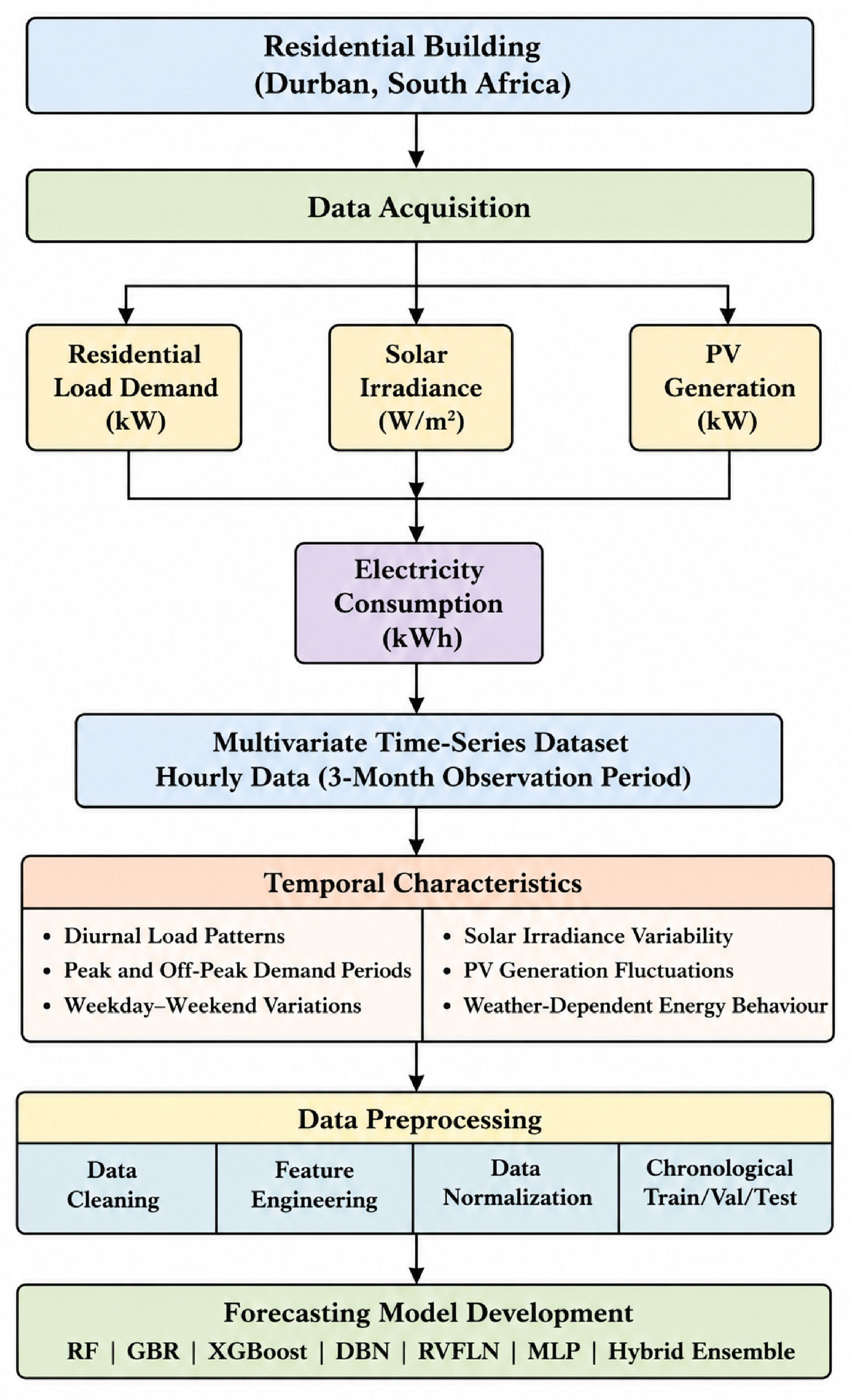
  63. Group, K. Durban at a Glance. Available online: https://www.kamdargroup.co.za/area-profiles/durban/ (accessed on 26 May 2026).
  64. Durban, South Africa. Available online: https://www.google.com/maps/place/Durban,+South+Africa (accessed on 15 May 2026).
  65. Spark, W. Climate and Average Weather Year Round in Durban KwaZulu-Natal, South Africa. Available online: https://weatherspark.com/y/96783/Average–Weather–in–Durban–KwaZulu–Natal–South–Africa–Year–Round#google_vignette (accessed on 24 May 2026).
  66. Eskom Fact Sheet. Available online: https://www.eskom.co.za/wp-content/uploads/2024/08/GX-0001-Generation-Plant-Mix-Rev-30.pdf (accessed on 15 April 2026).
  67. Britannica. Available online: https://www.britannica.com/place/Durban (accessed on 3 March 2026).
Figure 1. Overview of the dataset description and temporal characteristics framework adopted in this study.
Energies 19 04414 g001
Figure 2. Data collection and preprocessing.
Energies 19 04414 g002
Figure 3. Framework of feature engineering.
Energies 19 04414 g003
Figure 4. Forecasting models for multi-target residential energy system.
Energies 19 04414 g004
Figure 5. Random forest forecasting architecture.
Energies 19 04414 g005
Figure 6. Architecture of gradient boosting regression.
Energies 19 04414 g006
Figure 7. Architecture of extreme gradient boosting.
Energies 19 04414 g007
Figure 8. Architecture of deep belief networks.
Energies 19 04414 g008
Figure 9. Architecture of RVFL network.
Energies 19 04414 g009
Figure 10. Architecture of multi-layer perceptron.
Energies 19 04414 g010
Figure 11. Architecture of hybrid ensemble forecasting framework.
Energies 19 04414 g011
Figure 12. Model performance evaluation framework for residential load demand, solar PV and electricity bill forecasting.
Energies 19 04414 g012
Figure 13. Geographical location of the selected site [67].
Energies 19 04414 g013
Figure 14. Monthly average global solar irradiance and ambient temperature profile of Durban, South Africa.
Energies 19 04414 g014
Figure 15. Residential energy system in Durban, South Africa.
Energies 19 04414 g015
Figure 16. Analysis of load demand, solar irradiance, solar energy generation and electricity bill of residential building.
Energies 19 04414 g016
Figure 17. Comparative performance of residential load demand forecasting across various models.
Energies 19 04414 g017
Figure 18. Hourly distribution error for load demand based on different models.
Energies 19 04414 g018
Figure 19. Comparative performance of residential load demand forecasting models across individual evaluation metrics using radar charts: (a) MAE; (b) RMSE; (c) MSE; (d) R2 and (e) MASE.
Energies 19 04414 g019
Figure 20. Comparison of solar irradiance forecasting based on different models.
Energies 19 04414 g020
Figure 21. Hourly error distribution analysis of solar irradiance forecasting models.
Energies 19 04414 g021
Figure 22. Comparative performance of solar irradiance forecasting models across individual evaluation metrics using radar charts: (a) MAE; (b) RMSE; (c) MSE; (d) R2 and (e) MASE.
Energies 19 04414 g022aEnergies 19 04414 g022b
Figure 23. Comparison of solar energy forecasting based on different models.
Energies 19 04414 g023
Figure 24. Hourly error distribution analysis of solar energy forecasting models.
Energies 19 04414 g024
Figure 25. Comparative performance of solar energy forecasting models across individual evaluation metrics using radar charts: (a) MAE; (b) RMSE; (c) MSE; (d) R2 and (e) MASE.
Energies 19 04414 g025
Figure 26. Comparison of electricity bill forecasting based on different models.
Energies 19 04414 g026
Figure 27. Hourly error distribution analysis of electricity bill forecasting models.
Energies 19 04414 g027
Figure 28. Comparative performance of residential load demand forecasting models across individual evaluation metrics using radar charts: (a) MAE; (b) RMSE; (c) MSE; (d) R2 and (e) MASE.
Energies 19 04414 g028
Figure 29. Radar chart comparison of forecasting models across: (a) Load demand (b) Solar irradiance (c) Solar energy and (d) Electricity bill.
Energies 19 04414 g029
Table 1. Statistical error analysis for load demand.
ModelMeanErrRangeStdDevSkewnessKurtosis
Hybrid Ensemble−0.000131860.810930.1160.344483.6003
XGBoost−0.00013880.853610.12210.344483.6003
GBR−0.000125150.971010.140260.350483.583
RF−0.00043711.10930.1580.364383.6505
RVFL−0.0012141.21530.183270.310783.4525
MLP0.00330351.38680.209940.270953.3586
DBN0.00341771.64520.247410.290673.5096
Table 2. Performance evaluation of load demand forecasting models.
ModelMAERMSEMSER2MASE
Hybrid Ensemble0.0905220.115870.0134250.983440.28023
XGBoost0.0952860.121960.0148750.981660.29498
GBR0.109660.14010.0196280.97580.33947
RF0.123030.157820.0249070.969280.38086
RVFL0.143810.183070.0335130.958670.44518
MLP0.166010.209730.0439860.945760.5139
DBN0.193590.247150.0610830.924670.59929
Table 3. Statistical error analysis for solar irradiance.
ModelMean ErrorRangeStdDevSkewnessKurtosis
Hybrid Ensemble−1.0877 × 10−180.00424220.000780.030782.8341
XGBoost1.4291 × 10−190.00606180.0011167−0.121032.8865
GBR−1.0083 × 10−180.00875830.0014533−0.168263.0474
RF−1.9054 × 10−190.0109480.00179−0.16213.1443
RVFL−1.0604 × 10−180.0119010.00212670.0292722.6848
MLP−3.9696 × 10−190.0162460.0024633−0.0686093.3836
DBN−1.1353 × 10−180.016380.00280.182222.7088
Table 4. Performance evaluation of solar irradiance forecasting models.
ModelMAERMSEMSER2MASE
Hybrid Ensemble0.219690.369760.136720.988790.0034927
XGBoost0.231260.389220.151490.987580.0036765
GBR0.272290.448630.201270.98350.0043289
RF0.3130.507640.257690.978870.0049761
RVFL0.372080.583110.340020.972120.0059154
MLP0.441390.671340.450690.963050.0070173
DBN0.51990.771450.595130.951210.0082525
Table 5. Statistical error analysis for solar energy.
ModelMeanErrRangeStdDevSkewnessKurtosis
Hybrid Ensemble0.00365240.0315560.00555441.26194.0469
XGBoost0.00384460.0332170.00584671.26194.0469
GBR0.00445030.0378530.00673491.2584.0197
RF0.00500070.042640.00758441.22833.9568
RVFL0.00576920.0490770.0087871.2033.9374
MLP0.00657470.0602490.0101931.15793.9313
DBN0.00733780.0623060.0117641.11353.8112
Table 6. Performance evaluation of solar energy generation forecasting models.
ModelMAERMSEMSER2MASE
Hybrid Ensemble0.00394870.00664234.412 × 10−50.988840.34876
XGBoost0.00415660.00699194.8887 × 10−50.987630.36712
GBR0.00489260.0080666.5061 × 10−50.983540.43212
RF0.00561190.00907748.2399 × 10−50.979150.49565
RVFL0.00674040.0105030.000110320.972090.59533
MLP0.00798140.012120.000146880.962830.70494
DBN0.00938140.0138530.000191910.951440.82859
Table 7. Statistical error analysis for electricity bill.
ModelMeanErrRangeStdDevSkewnessKurtosis
Hybrid Ensemble0.000300150.155670.0229850.238753.1317
XGBoost0.000315950.163860.0241950.238753.1317
GBR0.000376790.189310.0278530.244463.1638
RF0.000358790.21330.0314830.232953.1343
RVFL9.8036 × 10−50.23970.0366050.273153.1592
MLP0.000305520.295980.0420340.215623.3839
DBN0.000917450.318460.049740.126093.1588
Table 8. Performance evaluation of electricity bill forecasting models.
ModelMAERMSEMSER2MASE
Hybrid Ensemble0.0181260.0229610.000527190.979780.30006
XGBoost0.019080.0241690.000584140.977590.31585
GBR0.0220020.0278690.000776660.970210.36421
RF0.0249060.0290800.0009940.961870.4123
RVFL0.0285610.0360350.00129850.950190.4728
MLP0.0333580.0421210.00177420.931940.5522
DBN0.0391090.0489570.00239680.908060.64741
Disclaimer/Publisher’s Note: The statements, opinions and data contained in all publications are solely those of the individual author(s) and contributor(s) and not of MDPI and/or the editor(s). MDPI and/or the editor(s) disclaim responsibility for any injury to people or property resulting from any ideas, methods, instructions or products referred to in the content.