A Comprehensive Database and Smart-Learning Framework for Monitoring Failure Risk Factors, Maintenance, and Protection in Electrical Networks

Abstract

Electrical power systems are exposed to interacting electrical, thermal, environmental, and resource-related faults such as leakage current, voltage and frequency deviations, overcurrent, harmonic distortion, phase-sequence error, humidity, fire, wind-speed variability, water insufficiency, and solar-resource loss. This study introduces a software-based database-generation and smart-learning framework that converts 22 candidate risk factors into six normalized severity levels and then maps the simultaneous system state to low-, medium-, and high-level protection decisions. The main novelty is that the software not only evaluates existing measurements; it also produces a literature- and standards-informed synthetic database when long-term real field measurements are not yet available. The database is generated by defining variable limits, sampling realistic operating states, computing severity labels, and storing input–output pairs that can later train or validate predictive maintenance models. The proposed framework therefore, links protection logic, database construction, and reusable training data in a single workflow. The results show how simulated annual operating scenarios can be transformed into structured risk records, warning classes, and shutdown decisions, supporting early fault detection, maintenance planning, and resilience improvement in renewable-integrated electrical networks.

1. Introduction

Electric power grids are becoming increasingly complex due to the integration of conventional generation, distributed renewable energy sources, variable loads, and advanced protection devices. This study was undertaken for two practical reasons. First, obtaining comprehensive fault databases for electrical power systems is difficult because severe faults occur infrequently, are unsafe to reproduce experimentally, and often require long observation periods to capture. Second, predictive maintenance and intelligent protection algorithms require labeled datasets for effective training and validation; therefore, an initial database must be established before these learning systems can be successfully developed.

To address this need, a software framework was developed to generate and evaluate 22 candidate risk factors, including voltage deviations, current faults, frequency variations, harmonic distortion, phase-sequence abnormalities, temperature, humidity, flame, earthquake, fuel conditions, wind speed, solar radiation, and water-related variables. Each parameter is classified into a six-level severity scale according to literature-based thresholds and system-oriented engineering criteria.

The novelty of this study is threefold. First, it introduces a unified database structure that combines electrical, thermal, environmental, and renewable energy-related risk factors within a single framework. Second, the proposed software generates synthetic yet realistic data when long-term field measurements are unavailable or insufficient. Third, the generated records are automatically converted into alert labels that can be used to train, test, and continuously improve intelligent protection systems and decision-making algorithms.

The proposed database is not intended to replace real-world measurements. Instead, it provides an initial training and evaluation platform for the development of smart monitoring and protection applications. As new operational data become available, they can be incorporated into the existing database, compared with previously generated records, and used to refine the decision boundaries and improve the performance of intelligent protection algorithms.

To preserve the full original literature coverage in a shorter introduction, the reviewed studies are now grouped compactly as follows: renewable-energy integration, hybrid solar-PV/wind uncertainty, load and generation forecasting, microgrid energy management, AI-/quantum-assisted renewable integration, and real-time scheduling are represented by [1,2,3,4,5,6,7]; wind-energy, hydropower, environmental-variable, and decarbonization impacts are represented by [8,9,10,11,12,13]; and smart-learning/ML-based monitoring, including digital-twin PV fault detection, embedded ML, wind-turbine diagnosis, harmonic-distortion detection, transmission/distribution fault localization, islanding detection, and power-quality disturbance classification, is represented by [14,15,16,17,18,19,20,21,22,23]. Together, these studies motivate the proposed contribution: instead of presenting only another classifier, this paper focuses on producing a traceable database-generation and alert-labeling pipeline that can support future learning-based protection and maintenance systems [24,25,26,27,28,29].

Table 1. Summary of ML-based fault detection studies.

Reference (Authors, Year)	Focus	Key Findings
Ibrahim et al. [25]	Machine learning applications in smart power systems	ML enables the transformation of conventional grids into smart, self-healing systems through improved fault detection, forecasting, and control.
Ozcanli et al. [22]	Deep learning in electrical power systems	Deep learning models outperform classical ML in complex tasks but require large datasets and careful training.
Furse et al. [19]	Fault diagnosis in electrical power systems	Transition from model-based methods to data-driven ML approaches improves diagnostic performance in complex systems.
Cao et al. [16]	ML-based fault detection in solar PV with digital twin	Digital twin-based ML enables real-time, accurate fault detection and localization in large-scale PV systems.
Kaitouni et al. [26]	Digital twin-assisted fault detection in urban PV systems	Combining digital twin models with ML improves fault sensitivity and reduces false alarms.
Pujara et al. [28]	Embedded ML for PV fault detection	Lightweight ML models enable real-time fault detection at the edge with reduced communication overhead.
Allal et al. [14]	Two-tier ML framework for wind turbine faults	Hierarchical ML improves accuracy and robustness in wind turbine fault detection and classification.
Ding et al. [17]	AI-based abnormal detection in wind systems	Adaptive AI systems enable automatic feature extraction and robust anomaly detection under varying conditions.
Elshenawy et al. [18]	Comparative ML methods for wind turbine fault detection	No single ML model dominates; performance depends on data and fault type, encouraging hybrid approaches.
Jove et al. [20]	Harmonic distortion detection in wind generators	ML-based harmonic analysis improves early detection of converter-related faults.
Anwar et al. [24]	Ensemble ML for transmission line fault detection	Ensemble models improve robustness and accuracy across varying fault conditions.
Najafzadeh et al. [27]	ML-based fault localization in power grids	Optimized ML models enable precise fault location, improving maintenance and restoration speed.
Moloi et al. [21]	SVM-based fault detection in distribution systems with DG	SVM effectively detects faults in systems with bidirectional power flow where traditional methods fail.
Panigrahi et al. [23]	Intelligent islanding detection methods	ML-based approaches outperform classical methods in distinguishing islanding conditions.
Satyanrayana et al. [29]	Power quality disturbance classification	Combining signal processing with ML achieves high accuracy in detecting disturbances like harmonics and transients.

summarizes representative studies on machine-learning-based fault detection and intelligent monitoring in renewable-integrated electrical power systems [30,31,32]. These studies demonstrate the need for large, well-structured, and interpretable datasets, but they generally do not provide a unified mechanism that simultaneously creates a database and converts multi-factor system states into protection outcomes. The compact grouping above preserves all original citations while keeping the introduction concise [21,33,34,35].

The literature indicates that machine learning, digital twins, and embedded diagnostic systems improve fault detection, but their performance depends strongly on the availability of labeled and representative data. Therefore, this work focuses on the missing data-generation step and presents a repeatable procedure for producing initial training records before large field datasets have been collected [32,36,37,38].

Accordingly, the study contributes a database-oriented protection methodology rather than only a classifier. The generated database records contain input variables, normalized severity levels, repetition counts, and final alert outcomes, which together form a reusable basis for future supervised learning, scenario analysis, and preventive maintenance planning.

2. Electrical Energy Systems and Faults

An electrical power system operates as an integrated chain of generation, transmission, distribution, protection, and load components. If any part of this chain deviates from its normal operating range, the disturbance may propagate to other parts of the network. Figure 1 illustrates typical fault categories that motivate the proposed multi-parameter monitoring approach.

If an electrical system works normally, electricity energy will reach everywhere normally, but if any error occurs, even a simple expected or unexpected one, it may lead to problems that may be serious and may lead to deprivation areas of electricity. These errors cause a decrease in the efficiency of the system, increased losses and costs, instability of electricity distribution, and dissatisfaction of consumers. When it comes to providing electricity to everyone, it is important to protect the environment, study climate change, and remove carbon when producing electricity, which directs us to the need to use renewable and alternative energy sources and integrate them into the electricity generation system to reduce the use of traditional sources.

When it comes to providing electricity to everyone, it is important to protect the environment, study climate change, and remove carbon when producing electricity, which directs us to the need to use renewable and alternative energy sources and integrate them into the electricity generation system to reduce the use of traditional sources. In this work, we will study potential faults that may occur in electrical energy systems and try to predict unexpected problems that may appear in the electricity system, which includes alternative energy systems such as wind and solar energy. Additionally, we will try to ensure that energy production and transmission processes are based on more reliable foundations, using algorithms supported by smart learning and detect and solve these errors.

Fault detection in electrical energy systems is critical to ensure the system’s safe, efficient, and continuous operation. Fault detection is usually achieved by using multiple methods and technology together. As shown in Figure 2, fault detection methods in electrical energy systems can be summarized as follows.

Protection systems of electrical energy systems are designed to quickly detect faults that may occur in the electrical network (short circuit, overload, grounding, etc.), to prevent the damage from growing and to protect the rest of the system. In this way, both life and property safety is ensured, and it is possible for electricity distribution to continue uninterrupted.

As required by the study, potential faults that may occur in electrical energy systems are investigated, and possible unexpected problems in systems integrating renewable energy sources such as water, wind and solar energy are predicted. The aim is to enhance the reliability of energy generation and transmission processes by utilizing smart learning-based algorithms for fault detection and mitigation. For this purpose, a software-based environment is employed to simulate real operating conditions and process large volumes of generated data. The analyses are carried out through simulation studies using a main program called secur along with 22 sub-programs representing various fault scenarios in renewable-integrated power systems.

These simulations are conducted by defining the coefficients and equations that characterize potential distortions in each system component. As a result, the study aims to achieve clean sinusoidal waveforms, stable current and voltage levels, and an overall reliable and balanced electrical network.

Artificial intelligence (AI) and machine learning (ML) provide essential tools for ensuring the continuous and reliable operation of power systems. These technologies enable critical tasks such as error prediction, anomaly detection, and fault classification. AI models can predict potential faults based on historical data, while ML algorithms learn normal system behavior to identify anomalies. In addition, classification algorithms can determine the type of faults, such as short circuits or phase losses, improving the effectiveness of diagnostic processes.

Various models are commonly used for fault prediction and analysis. Neural networks are capable of learning from large datasets to predict failures, while clustering techniques help identify similar fault patterns. Time series analysis is applied to estimate when faults may occur, and regression analysis evaluates the probability of faults based on historical trends. Furthermore, classification methods such as support vector machines and decision trees play a significant role in identifying system changes and enhancing testing accuracy.

Fault location in power systems can be achieved through several intelligent methods. AI-based techniques such as genetic algorithms, artificial neural networks, fuzzy logic, and support vector machines utilize measurement sensors, system data and environmental conditions to accurately locate faults in distribution networks (Figure 3).

Testing and simulation are fundamental for analyzing system behavior and predicting faults. Physical testing of equipment allows comparison with normal operating conditions, while simulation software enables modeling of fault scenarios in a controlled environment. These approaches allow us to evaluate system performance and anticipate potential issues before they occur.

Detection of a fault is critical for maintaining reliable energy systems in an electrical energy system. The integration of AI, ML, and advanced monitoring technologies enables more accurate, efficient, and proactive fault detection and prediction. These methods can be applied individually or in combination, depending on system complexity, and their effectiveness continues to increase with the advancement of AI and IoT technologies.

3. Detection of Electrical Energy System Faults by Using Software

In the study carried out, it was aimed to create an algorithmic and software approach towards sustainability for electrical energy systems including renewable energy production systems. The algorithm and software developed at this stage of the study were carried out on the creation of the basic algorithm and software for the evaluation of data obtained from the infrastructures forming the system. The algorithm and software developed up to this stage are aimed at determining the existence or non-existence of negativities in the infrastructure forming the electrical energy system. After this stage, studies on the algorithm and software will continue and the focus will be on the analysis of negativities that may occur in the electrical energy system infrastructure including renewable energy production systems in different scenarios.

In the analyses to be carried out after this stage, the effects of the input parameters listed in

Table 2. Scenarios of faults.

No.	Scenario	No.	Scenario
1	Present of earthquake.	12	Low frequency distortion.
2	Present of flame.	13	Low material temperature.
3	Status of fuel.	14	Low sine wave distortion.
4	High frequency distortion.	15	Low voltage.
5	Excessive hot material temperature.	16	Excessive cold weather.
6	Excessive hot weather.	17	Low wind speed.
7	Present of high wind speed.	18	Over current.
8	Present of high sine wave distortion.	19	Over voltage.
9	Present of humidity.	20	Phase sequence distortion.
10	Leakage current.	21	Insufficient water.
11	Present of excessive load.	22	Present of sun energy.

will be considered separately for the sustainability of the system, and the classifications of these parameters will be made. In these classifications, mathematical analysis of the effects of each parameter for the sustainability and usability of the system will be tried to be presented. Although the methods and analyses used in the study are carried out on a sample system, they can be adapted to different systems. Thus, it is thought that the results to be obtained will be a new contribution to the literature, as they will be able to concretely reveal the reliability of electrical energy systems, including renewable energy production systems. Explanations regarding the fault and sustainability parameters in the energy system can be seen in

Table 3. Descriptions of fault and sustainability parameters in the energy system.

Category	Parameter	Description (Software/System Oriented)
Electrical	Low Voltage	Voltage drops below nominal level; reduces efficiency and equipment performance
Electrical	Over Voltage	Risk of insulation damage and electronic component failure
Electrical	Over Current	Indicates overload or short circuit; fire and equipment damage risk
Electrical	Leakage Current	Insulation degradation or moisture-related safety hazard
Electrical	Phase Sequence Distortion	May cause reverse motor rotation and mechanical damage
Electrical	Low Sine Wave Distortion	Indicates weak loading or measurement instability
Electrical	High Sine Wave Distortion	Harmonic distortion causing losses and equipment overheating
Electrical	Low Frequency Distortion	Indicates generation–load imbalance affecting grid stability
Electrical	High Frequency Distortion	Switching noise and EMI affecting control and communication systems
Thermal	Low Material Temperature	Causes mechanical brittleness and battery efficiency reduction
Thermal	Excessive High Material Temperature	Leads to thermal stress, insulation failure, and fire risk
Load/Source	Excessive Load Presence	System operating beyond rated capacity; sustainability risk
Load/Source	Fuel Status	Critical for continuity of energy supply in generator or hybrid systems
Environmental	Earthquake Presence	Risk of physical infrastructure damage and sudden outages
Environmental	Excessive Hot Weather	Increases cooling demand and reduces system efficiency
Environmental	Excessive Cold Weather	Degrades battery, fuel, and mechanical performance
Environmental	Low Wind Speed	Insufficient wind energy generation potential
Environmental	High Wind Speed Presence	Increased generation potential but higher structural risk
Environmental	Humidity Presence	Causes corrosion, leakage current, and insulation degradation
Environmental	Solar Energy Presence	Indicates photovoltaic generation potential
Environmental	Insufficient Water	Risk for cooling systems, hydro power, and fire safety
Safety	Flame Presence	Early fire indicator; requires immediate alarm and shutdown

.

The frequency of occurrence of 22 variables can vary from person to person. How should these entities be defined? A separate study, based on the literature and sources, is being conducted within the study to determine the frequency of occurrence of each of these entities. The frequency of occurrence of the 22 data points considered in the electrical energy system will not be uniform, both statistically and in the literature. The determination supports the frequency of occurrence of the 22 data points considered in this context in

Table 4. Determination studies for the frequency of occurrence of 22 variables.

Category	Parameter	Normal/Acceptable Level (Typical)	Notes for 6-Level Input (0–6)	Key Literature/Standards (Examples)
Electrical	Low Voltage	LV supply voltage typically within ±10% of nominal (e.g., 230 V system: ~207–253 V) for most of the week.	Map 1 = within band, 2–3 = mild undervoltage, 4–6 = deep/prolonged undervoltage	EN 50160 (voltage variation statistical limits).
Electrical	Over Voltage	OV supply voltage typically within ±10% of nominal (same band as above); overvoltage = above that band.	1 = within band; higher levels by magnitude + duration	EN 50160.
Electrical	Low Frequency Distortion	Grid frequency (interconnected systems): 49.5–50.5 Hz (10 s mean) for 99.5% of a week; outside = abnormal.	Use deviation (Hz) + persistence (seconds/minutes)	EN 50160 summaries and guidance.
Electrical	High Frequency Distortion	Same normal band as above: 50–50.5 Hz (10 s mean) for interconnected systems.	Where the variable denotes EMI/high-frequency conducted disturbances, it is treated separately (see IEC 61000-2-2).	EN 50160 (frequency); IEC 61000-2-2 (conducted disturbances compatibility levels).
Power Quality	Low Sine Wave Distortion	Voltage waveform “normal” typically means harmonic voltage distortion within standard limits (THD-V). For LV: THD often ≤8% (IEEE 519).	1 = THD within limit; levels 2–6 by %THD and time	IEEE 519-2022 voltage distortion limits.
Power Quality	High Sine Wave Distortion	Typical “acceptable” THD-V limits by bus voltage: ≤1 kV: THD 8%, 1–69 kV: 5%, 69–161 kV: 2.5% (IEEE 519).	The PCC voltage level is used to select the limit; severity is mapped by the margin over the limit	IEEE 519-2022 Table (voltage THD).
Power Quality/EMC	High-Frequency Conducted Disturbance	Compatibility levels for conducted disturbances in LV networks are addressed in IEC 61000-2-2 (0–9 kHz, with extension for signaling).	Use measured band (kHz), amplitude (dBµV/%) and compare to compatibility level	IEC 61000-2-2 scope/compatibility levels.
Electrical	Over Current	“Normal” is ≤rated current for equipment; many protection practices treat continuous operation below nameplate (often ~80% for standard breakers in some regimes).	1 = below continuous design band; 5–6 = sustained overload/instantaneous fault	Practical guidance on 80% vs. 100% rated breakers (industry notes).
Electrical	Leakage Current	For personnel protection, RCD sensitivity ≤ 30 mA is widely used as “additional protection” threshold in IEC 60,364 context. (library.e.abb.com)	Levels are mapped using residual current bands (e.g., <5 mA, 5–15, 15–30, >30 mA)	IEC 60364-4-41 guidance via ABB technical guide/references. (library.e.abb.com)
Electrical/Safety	Touch/Equipment Leakage (device design view)	Some equipment standards commonly use 3.5 mA as a notable touch-current limit for certain classes; higher may be allowed with conditions. (advancedenergy.com)	Where equipment “touch current” is measured, it is separated from installation residual-current protection	IEC 950/EN 60950-1 discussion and leakage current notes (application notes). (advancedenergy.com)
Electrical	Phase Sequence Distortion	Normal = correct phase sequence (e.g., ABC) as required for intended rotation; wrong sequence implies reverse rotation risk. (Legal source)	1 = correct; 6 = incorrect (hard fault), or grade by detection confidence	IEC 60034-8 (connections/sequence and reversing rotation by swapping phases). (Legal source)
Thermal	Low Material Temperature	“Normal” depends on installation class; many stationary protected locations are described via IEC 60721-3-3 climate classes (temperature/humidity severities).	The target class is selected (e.g., controlled indoor vs. weather-protected) and levels 1–6 are mapped to that band	IEC 60721-3-3 (environmental parameter severities).
Thermal	Excessive High Material Temperature	Same approach: define acceptable band per equipment limits and environmental class; IEC 60721 helps define ambient severities for stationary installations.	Use manufacturer nameplate limits for windings/batteries; map severity by °C above limit	IEC 60721-3-3.
Environmental	Excessive Cold Weather	Use site climate class/design envelope (IEC 60721-3-3 provides classes for stationary installations, incl. weather-protected).	1 = within design envelope; 6 = outside envelope (icing/embrittlement risk)	IEC 60721-3-3 and related environmental engineering mappings.
Environmental	Excessive Hot Weather	Same as above—define normal envelope via IEC 60721 class and local design.	Severity by ambient °C and duration	IEC 60721-3-3.
Environmental	Humidity Presence	Define acceptable RH band by installation class; IEC 60721-3-3 classifies humidity severities for stationary installations.	Map 1–6 by RH% and condensation/icing risk flags	IEC 60721-3-3; example industry climate-class guidance derived from it.
Environmental/Wind	Low Wind Speed	For wind generation context, cut-in speeds around ~3 m/s are common; below cut-in = low/no generation.	1 = above cut-in; higher levels by sustained below cut-in (sustainability/availability impact)	Typical cut-in discussion + turbine model specs example.
Environmental/Wind	High Wind Speed Presence	Many turbines have cut-out ~25 m/s (example spec); above implies shutdown/structural risk.	1 = within operating range; 6 = above cut-out/survival conditions	Turbine spec example; planning docs showing cut-out norms.
Environmental/Wind (Design)	Wind Speed Design Class ()	IEC 61400-1 [41] defines design classes and external conditions framework for turbines (site suitability/design).	Levels 1–6 are mapped to the exceedance likelihood of the selected IEC class	IEC 61400-1 (design requirements/classes).
Environmental/PV	Solar Energy Presence	PV “reference” irradiance commonly uses STC: 1000 W/m2 (and typically 25 °C cell temp); use this as a normalization point.	1 = night/very low irradiance; higher levels by irradiance bands (W/m2)	STC reference irradiance in PV standards guidance.
Environmental/Seismic	Earthquake Presence	Normal = no seismic event; thresholds are typically site-dependent. IEEE 693 defines seismic qualification levels used in substation equipment design/qualification.	Map 1 = no shaking; 4–6 based on PGA/response spectra exceedance (per site hazard)	IEEE 693 (seismic design/qualification of substations).
Safety	Flame Presence	Normal = no flame detected. NFPA 72 is the core code for fire alarm/signaling; flame detection performance requirements are referenced/used in industry practice.	5 = confirmed flame alarm; add intermediate levels for pre-alarm confidence	NFPA 72 overview + code references.
Load/Source	Fuel Status	“Normal” = above minimum reserve threshold required for autonomy target (hours/days); value is site-specific (tank size, consumption, criticality).	Map 0 = full/healthy; 6 = below reserve/imminent shutdown	(No single universal standard threshold; define by design autonomy + risk policy.)
Utilities/Cooling	Insufficient Water	“Normal” depends on use: cooling water, hydro resource, firewater tank, etc. Define minimum operating level/pressure/flow per plant design and safety case.	Map by % of minimum required flow/level and duration	(Strongly site-specific; standards depend on application—cooling vs. fire protection vs. hydro)
Load	Excessive Load Presence	Normal = operate within continuous design band; many engineering practices keep sustained loading below nameplate/thermal limits (e.g., typical 80% continuous for standard breakers in some regimes).	1 = normal band; 4–6 = sustained overload or repeated overload cycles	Industry guidance on continuous loading vs. breaker rating.

.

3.1. Mathematical Principles and Database-Generation Pipeline

The database is produced by mapping each measured or simulated physical variable into a common six-level severity domain. This prevents variables with different units, such as voltage, current, temperature, wind speed, and irradiance, from dominating the evaluation only because of their numerical scale. The transformation is direction-aware: variables whose risk increases with magnitude use direct normalization, whereas variables whose risk increases as the value decreases use an inverse normalization (Figure 4). Direct-risk normalization,

s_i(t) = 1 + 5 · (x_i(t) − x_i,_min)/(x_i,_max − x_i,_min), 1 ≤ s_i(t) ≤ 6.

(1)

This form is used for parameters such as overvoltage, overcurrent, leakage current, high temperature, high wind speed, humidity, flame, and earthquake intensity, where larger values represent larger risk. Inverse-risk normalization,

s_i(t) = 1 + 5 · (x_i,_max − x_i(t))/(x_i,_max − x_i,_min), 1 ≤ s_i(t) ≤ 6

(2)

This inverse form is used for parameters such as fuel availability, water availability, solar-energy availability, low wind speed, low voltage, and low temperature, where smaller values indicate a more critical operating condition. After normalization, each continuous severity value is rounded or clipped to the nearest integer level in the interval 1–6. Weighted global risk index,

R(t) = [Σ_i=1²² w_i s_i(t)]/[Σ_i=1²² w_i], w_i ∈ {1,2,3}.

(3)

The weight w_i is assigned from the priority level of the corresponding parameter. A high-priority safety variable, such as flame, leakage current, overcurrent, or phase-sequence distortion, therefore contributes more strongly to the global risk index than a low-priority resource-availability variable. The priority levels w ∈ {1,2,3} listed in

Table 5. Normal level ranges for six severity levels based on determination data.

Variable	Unit	Priority Level	Number of Scenarios	Limits
Present of earthquake	Richter	2	6	0 to 6
Present of flame	Centigrade	1	6	1 to 5
Present of fuel	Liter	1	6	5 to 35
High frequency distortion	Hz	2	6	49.6 to 50.4
Excessive hot material temperature	Centigrade	1	6	−20 to 60
Excessive hot weather	Centigrade	3	6	−10 to 40
Present of high wind speed	m/s	3	6	4 to 20
High sine wave distortion	-	3	6	310 to 330 218 to 230
Present of humidity		2	6	0 to 50
Leakage current	mA	1	6	0 to 30
Present of excessive load	A	1	6	50 to 95
Low frequency distortion	Hz	2	6	49.6 to 50.4
Low material temperature	Centigrade	1	6	−20 to 60
Low sine wave distortion	-	3	6	310 to 330 218 to 230
Low voltage	V	2	6	215 to 230
Excessive cold weather	Centigrade	3	6	−10 to 40
Low wind speed	m/s	3	6	4 to 20
Over current	A	1	6	45 to 75
Over voltage	V	2	6	215 to 230
Phase sequence distortion (L1–L2–L3)	-	1	6	123, 132, 213, 231, 321, 312
Insufficient water	Meter	3	6	5 to 20
Insufficient sun energy	Candela	3	6	25,000 to 110,000

are not assigned subjectively. They were derived from the severity classifications of the relevant protection standards (e.g., IEC 60364, IEC 61508/61511 safety-integrity reasoning, and IEEE C37 protection practice) together with the literature-based determination data summarized in Table 4. A factor is assigned the highest priority (3) when its exceedance can cause an immediate, irreversible, or life-threatening failure (e.g., flame, leakage current, overcurrent, and phase-sequence loss); an intermediate priority (2) when it degrades performance or accelerates aging without causing instantaneous failure (e.g., harmonic distortion, over-temperature, and humidity); and the lowest priority (1) when it primarily affects resource availability or generation margin rather than equipment integrity (e.g., wind-speed variability, solar-resource loss, and water insufficiency). This mapping makes the weighting reproducible and adjustable: when site-specific standards or measured failure statistics become available, the priority of any factor can be updated without altering the rest of the framework. The entire database record row is defined as follows,

D(t) = {x₁(t), …, x₂₂(t), s₁(t), …, s₂₂(t), R(t), C₁(t), …, C₆(t), y(t)}

(4)

For the energy-system input parameters considered in the study, the normal ranges determined for six severity levels, taking into account the determination information summarized in Table 4, are shown in Table 5.

3.2. Software-Based Creation of the Evaluation Database

Before the evaluation outcomes in

Table 6. Evaluation outcomes of the program.

Output Level	Number of Outputs	Program Comment	Number of Outputs	Program Comment	Number of Outputs	Program Comment
1	1:22	The system is in good condition (no warning)	-	-	-	-
2	1:14	Low Level Alert: “warning”	15:22	Medium Level Alert: “WARNING!”
3	1:11	Low Level Alert: “warning”	12:18	Medium Level Alert: “WARNING!”	19:22	High Level Alert: “STOP” (The Systems Shut Down)
4	1:7	Low Level Alert: “warning”	8:16	Medium Level Alert: “WARNING!”	17:22	(The Systems Shut Down)
5			1:6	Medium Level Alert: “WARNING!”	7:22	High Level Alert: “STOP” (The Systems Shut Down)
6					1:22	High Level Alert: “STOP” (The Systems Shut Down)

Note: If there are problems with renewable resources, then fuel-based production becomes necessary.

are produced, the software creates a database by executing four steps. First, it reads the minimum and maximum limits of each of the 22 variables from the literature-based range table. Second, it generates realistic random values within these ranges at predefined time intervals. Third, it converts each value into a six-level severity code using the normalization equations above. Fourth, it stores both the raw input value and the severity output as a paired database record.

This procedure allows the system to create new data from earlier generated data. When a new operating state is simulated or measured, the software compares the new variable vector with the existing severity ranges and previously labeled outcomes. The new record is then appended to the database, and the enlarged database becomes the basis for producing additional scenarios, recalibrating alert thresholds, and training future smart-learning models.

Table 6 was therefore created by grouping the 22 severity outputs according to the repetition counts of low-, medium-, and high-risk states. The table is not a manually assigned result table; it is the decision layer that translates database records into operational comments such as no warning, warning, WARNING!, and STOP. Critical warning levels may result from an evaluation of factors affecting the safe and reliable operation of electrical power systems. These factors include insufficient renewable energy generation, overload-induced changes in electrical and physical parameters, extreme variations in ambient temperature, and human-induced or natural events that adversely affect system performance.

As with nighttime hours in solar systems, even if negative data are generated during hours when energy production ceases for renewable energy systems, these data do not lead to the complete shutdown of the system, but rather to the activation of backup systems, such as fossil fuel-based production. Application studies on fault events involving the 22 variables are carried out using the variable limits in Table 5 and the alert-output logic in Table 6.

4. Application Results on Error Occurrences Involving 22 Variables in Electrical Energy Systems: Obtaining the Database

The parameters considered in the program were examined according to their potential to cause failures in the electrical energy system. For each parameter, the software first defines a physically meaningful operating interval and then assigns a six-level severity range based on the literature and standards summarized in Table 4 and Table 5.

It is quite acceptable for some regions of the world to have data below these ratios and for others to have data above them. The aim here is to conduct a study that considers average or slightly above-average failure risks.

When these criteria are considered in terms of environmental conditions, the program takes into account that earthquake and fire risks may occur in any environment, fossil fuels may be insufficient, hydroelectric water resources may decrease, sunless and windless days may occur, very low and high air temperatures may occur, storms may occur, and extreme rainfall and flood conditions may take place.

When considering the technical analysis of the operation of the electrical energy system, the program takes into account that, especially in regions where the interconnected system is not of sufficient size, frequency problems may occur, material temperatures may increase excessively for many facilities overloaded with the system, distortions in sine waves may occur, leakage currents may arise, overloading may occur, voltage drops and surges may occur, and overcurrent faults may occur.

Because this study is a simulation-based software application, the database is produced by generating time-stamped records for the 22 input variables. Each generated row contains the raw physical values, their six-level severity labels, the repetition counts of each level, and the final alert outcome. In this way, the software produces not only a set of examples but also a structured database that can be expanded with future real measurements. Sample tables taken from 1,314,900 for data points, randomly generated over a one-year period using instantaneous times (seconds), and their corresponding outputs are provided to be Appendix A, Appendix B and Appendix C.

The generated database has two functions. It provides an initial dataset for evaluating the proposed protection logic, and it creates a reusable training source for future smart-learning models. When new data are produced within the system, they are normalized and labeled using the same mathematical rules, appended to the previous records, and used to enrich the database for subsequent simulations.

Using the input data in

Table 7. Randomly generated values entered ten times with a half-hour interval between each run.

Names of Sub-Programs	Time
	12:39:21	13:09:21	13:39:21	14:09:21	14:39:21	15:09:21	15:39:21	16:09:21	16:39:21	17:09:21
Earthquake	1	5	1	4	2	5	0	3	4	4
Flame	1	5	5	2	2	4	1	5	3	3
Fuel	10	9	20	15	19	5	10	19	18	8
High frequency	49.97	50.22	50.07	49.94	50.35	50.30	50.08	50.45	50.33	50.24
High material temperature	56	60	52	36	56	37	20	27	34	25
High weather temperature	17	33	38	32	22	26	29	21	26	32
High wind speed	20	19	17	20	18	13	12	20	15	17
High sine wave	210	219	229	220	212	216	223	220	225	211
Humidity	17	28	28	38	20	12	43	31	21	7
Leakage current	22	8	22	12	8	10	30	25	21	0
Load	86	84	76	94	82	67	76	76	93	70
Low frequency	49.73	49.70	49.32	50.09	49.52	49.73	50.09	49.46	49.92	49.96
Low material temperature	8	6	−2	15	16	3	2	−2	8	5
Low sine wave	211	212	220	219	218	218	216	230	218	228
Low voltage	216	217	217	216	217	218	217	218	218	215
Low weather temperature	−9	−1	14	10	8	7	2	8	1	13
Low wind speed	5	11	11	11	11	12	4	10	4	4
Over current	68	70	72	73	65	68	73	59	55	63
Over voltage	227	227	224	226	226	224	220	225	229	221
Phases	312	123	231	231	132	321	213	231	123	231
River	14	5	18	7	12	7	18	7	18	5
Sun	31,008	72,587	10,434	10,147	85,673	30,139	58,535	72,775	31,635	90,168

and the output data in

Table 8. Output levels obtained by running 22 subprograms ten times with a half-hour interval.

Names of Sub-Programs	Time
	12:39:21	13:09:21	13:39:21	14:09:21	14:39:21	15:09:21	15:39:21	16:09:21	16:39:21	17:09:21
Earthquake	2	6	2	5	3	6	1	4	5	5
Flame	2	6	6	3	3	5	2	6	4	4
Fuel	4	4	1	3	2	6	4	2	2	5
High frequency	1	4	2	1	5	5	2	6	5	4
High material temperature	5	6	5	3	5	3	1	2	3	2
High weather temperature	1	4	6	4	2	3	3	2	3	4
High wind speed	6	6	5	6	5	2	1	6	4	5
High sine wave	1	3	6	1	1	1	6	3	5	1
Humidity	2	3	3	4	3	2	5	4	3	1
Leakage current	5	2	5	3	2	3	6	6	5	1
Load	4	4	3	5	4	2	3	3	5	3
Low frequency	3	3	6	1	4	3	1	5	2	2
Low material temperature	3	3	4	2	2	3	3	4	3	3
Low sine wave	6	4	1	1	4	1	3	1	1	1
Low voltage	5	4	4	5	4	3	4	3	3	6
Low weather temperature	6	4	1	2	2	2	3	2	3	1
Low wind speed	6	1	1	1	1	1	6	2	6	6
Over current	4	4	5	5	3	4	5	2	2	3
Over voltage	4	4	3	4	4	3	1	3	5	1
Phases	6	1	6	6	6	6	6	6	1	6
River	4	1	6	2	4	2	6	2	6	1
Sun	6	2	1	1	2	6	3	2	6	2

as the initial database, operational outputs for monitoring an electrical power system over a one-year operating period can be obtained. The following representations show author-generated software simulation graphs for 15 sample operating days (representing one year); these figures are produced from the database created by the proposed software. Since the developed software is capable of generating and continuously updating the database on a second-by-second basis, 15 representative parameters are graphically presented in Figure 5, Figure 6, Figure 7, Figure 8, Figure 9, Figure 10, Figure 11, Figure 12, Figure 13, Figure 14, Figure 15, Figure 16, Figure 17, Figure 18 and Figure 19. These graphs illustrate the variation in each parameter over time according to the predefined severity levels. Green and light green indicate normal operating conditions or minor deviations within acceptable limits, while yellow and orange represent moderate deviations requiring attention. Pink and red denote severe and critical deviations that exceed the predefined safety thresholds. The software evaluates these deviations both individually and collectively to generate the appropriate warning and alert information. It should be noted that these 15 examples represent 15 representative moments selected from an annual analysis period spanning one year. They are presented as illustrative examples drawn from the more than one million records contained in the full database, so as to demonstrate the behavior of the software without unduly increasing the length of the paper.

5. Evaluation of Application Results by the Program

For monitoring electrical energy systems, the random system inputs generated by the program in accordance with the literature for 15 monitoring points taken as a sample for one year of monitoring are given in

Table 9. Initial system information for 15 samples randomly generated from literature-based limits over a one-year period. Dates are given in the DD/MM/YY format (e.g., 19/01/25 denotes 19 January 2025).

Names of Sub-Programs	No	1	2	3	4	5	6	7	8	9	10	11	12	13	14	15
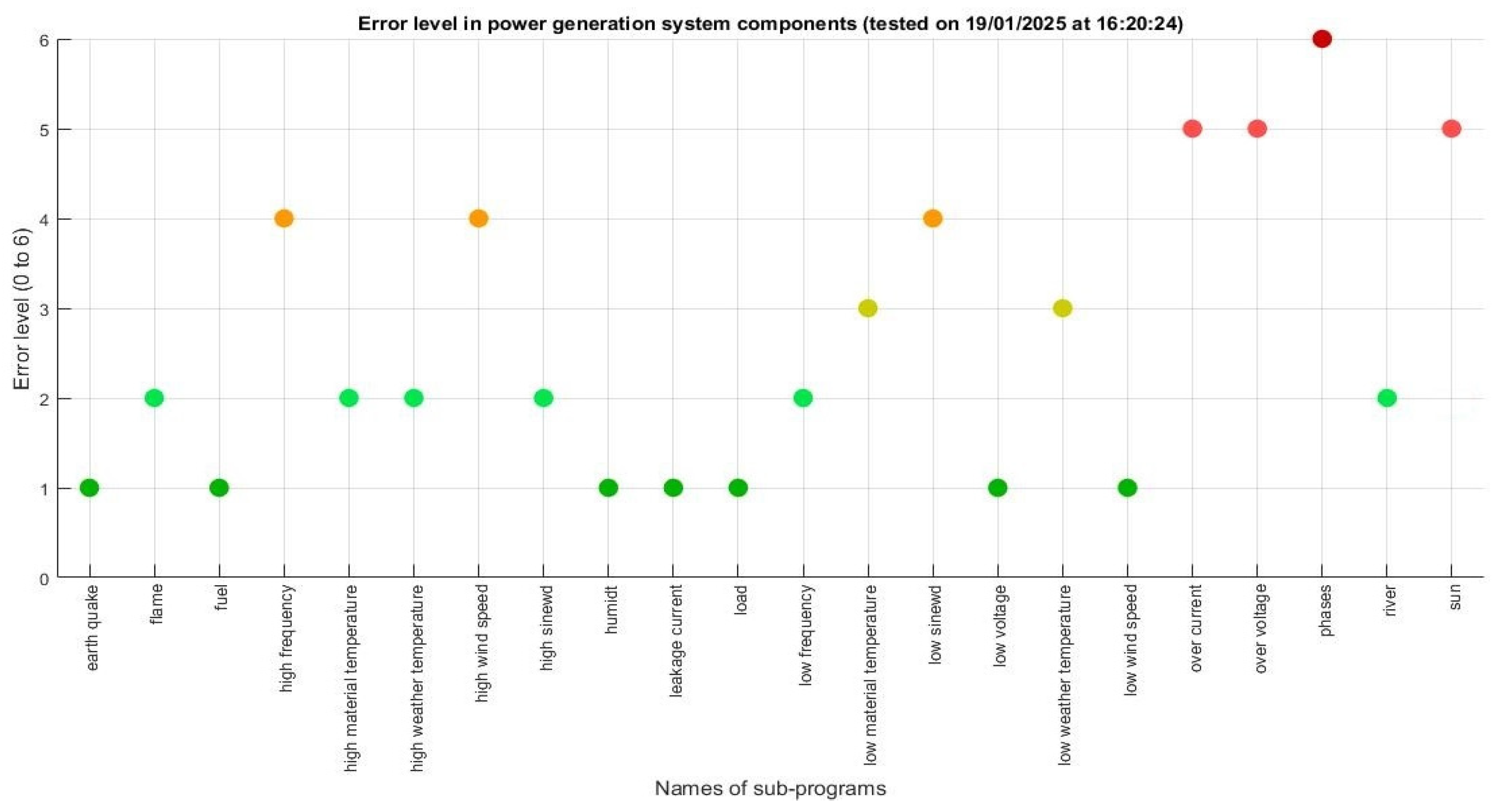
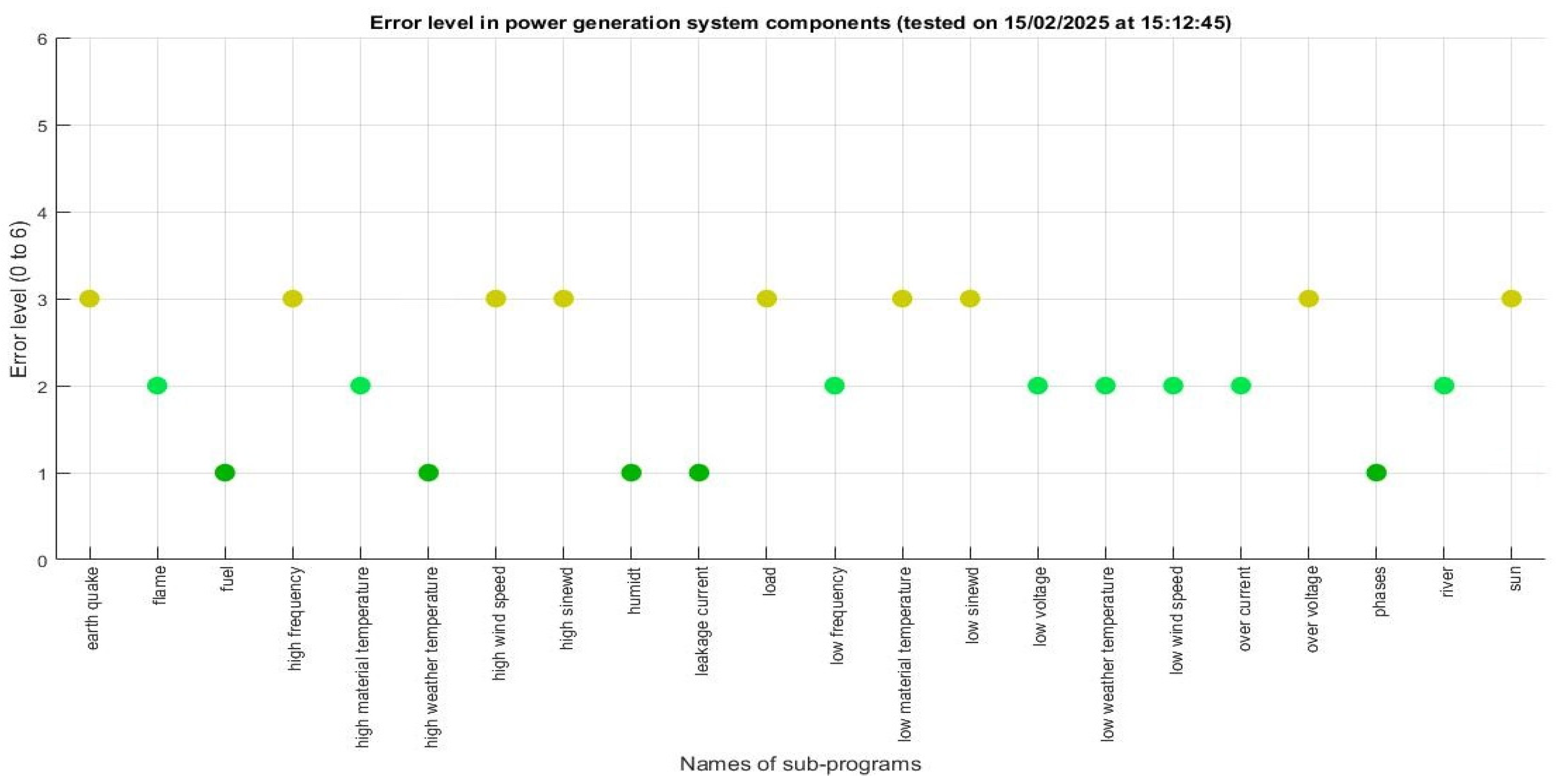
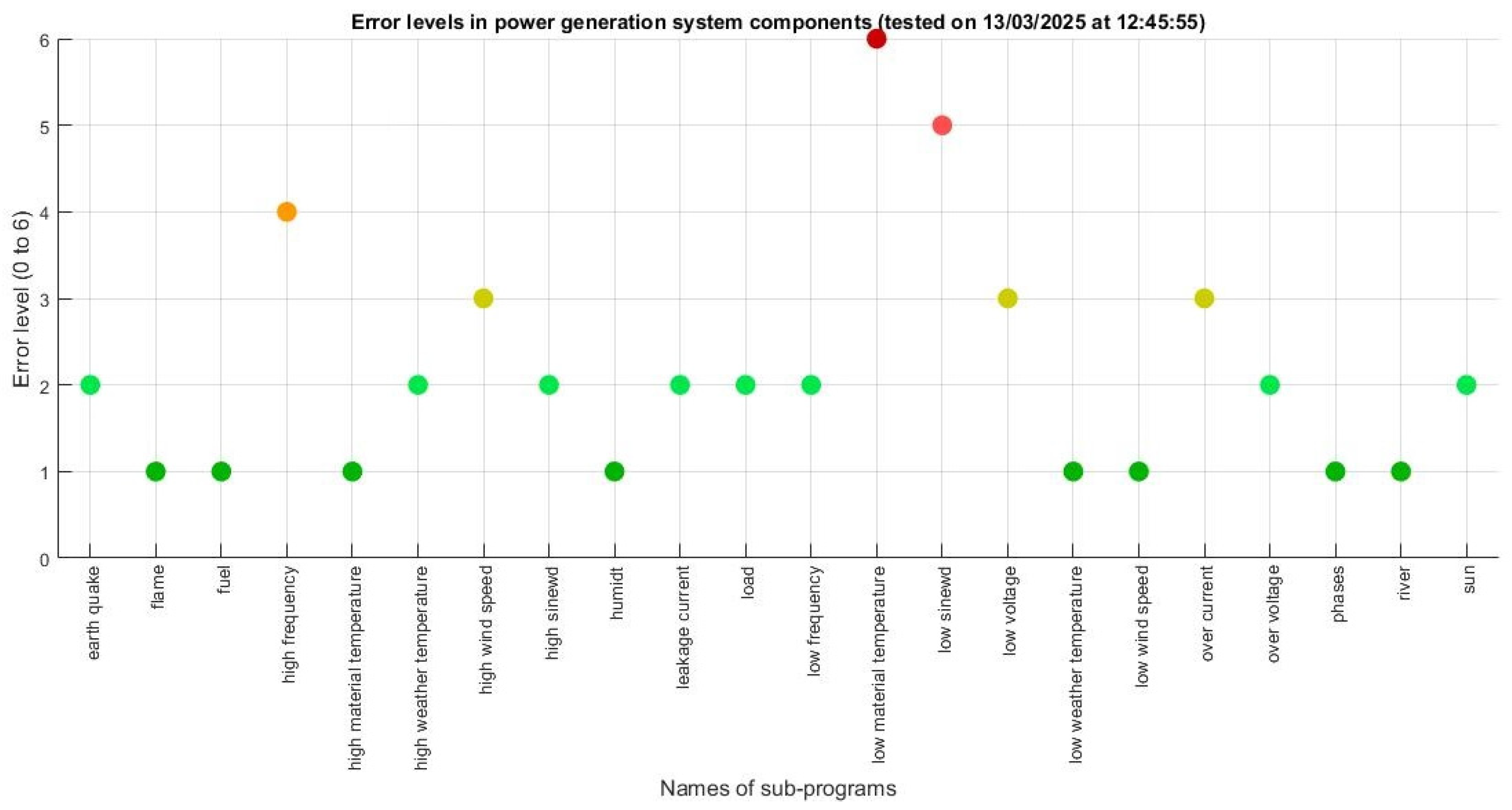
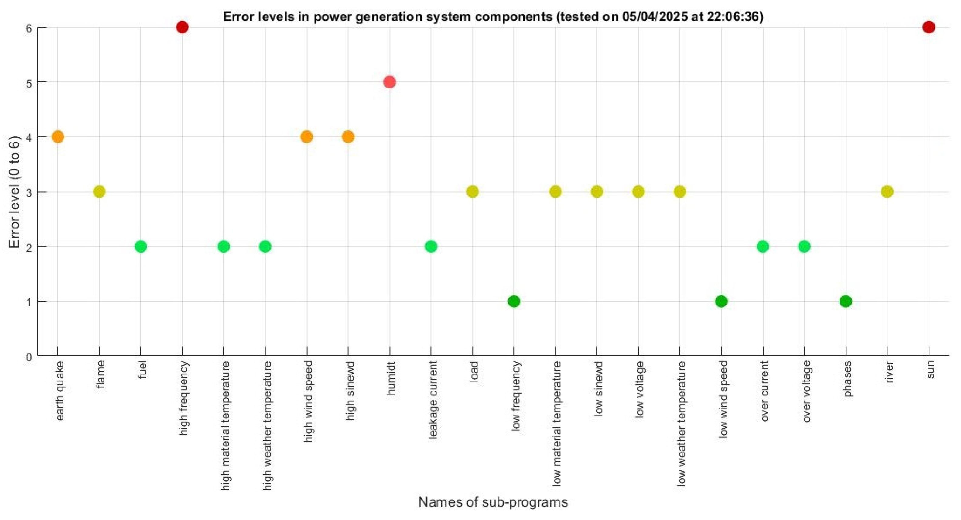
	Date	19/01/25	15/02/25	13/03/25	05/04/25	29/04/25	25/05/25	18/06/25	14/07/25	05/08/25	27/08/25	23/09/25	18/10/25	15/11/25	10/12/25	15/01/26
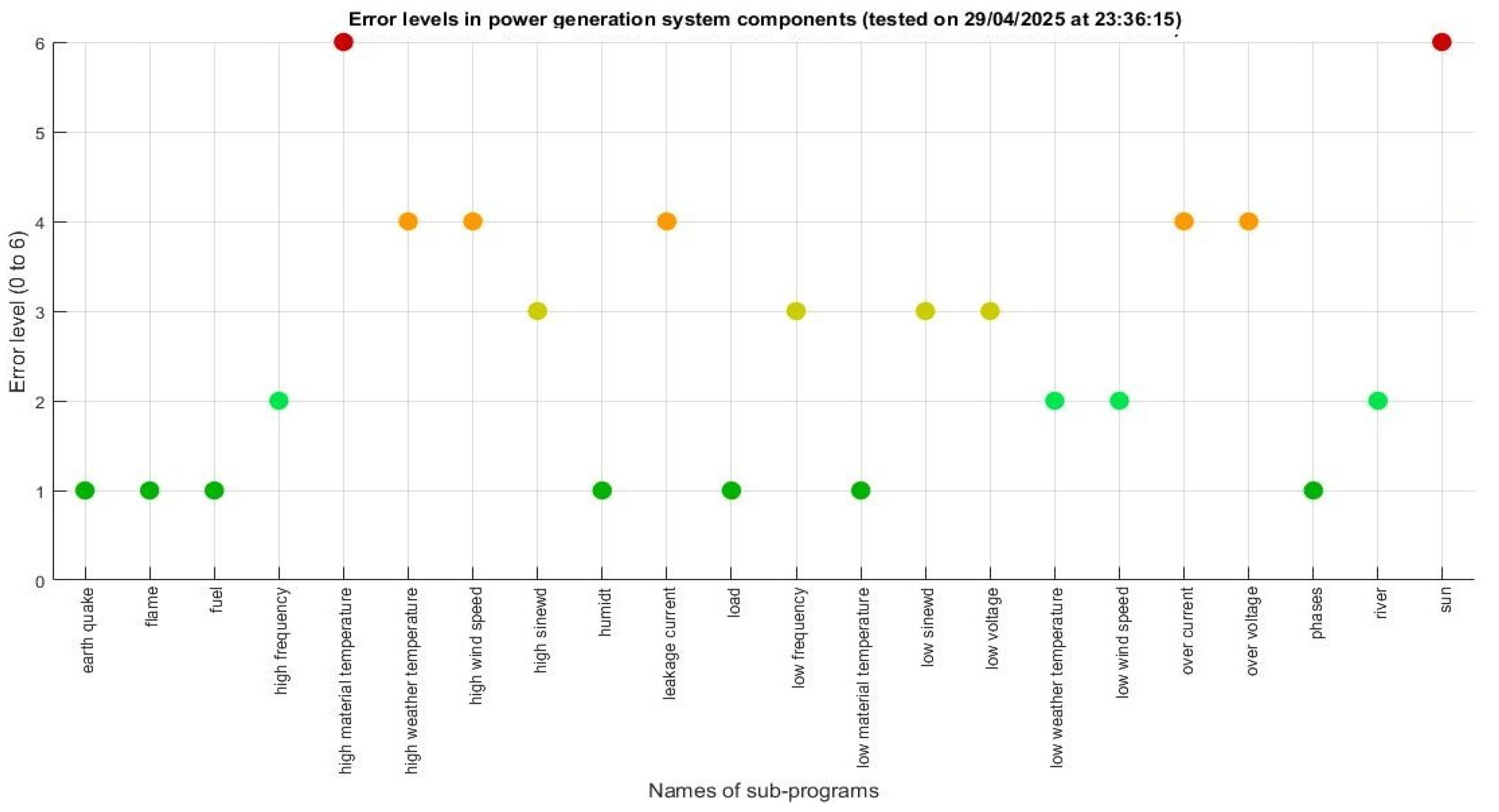
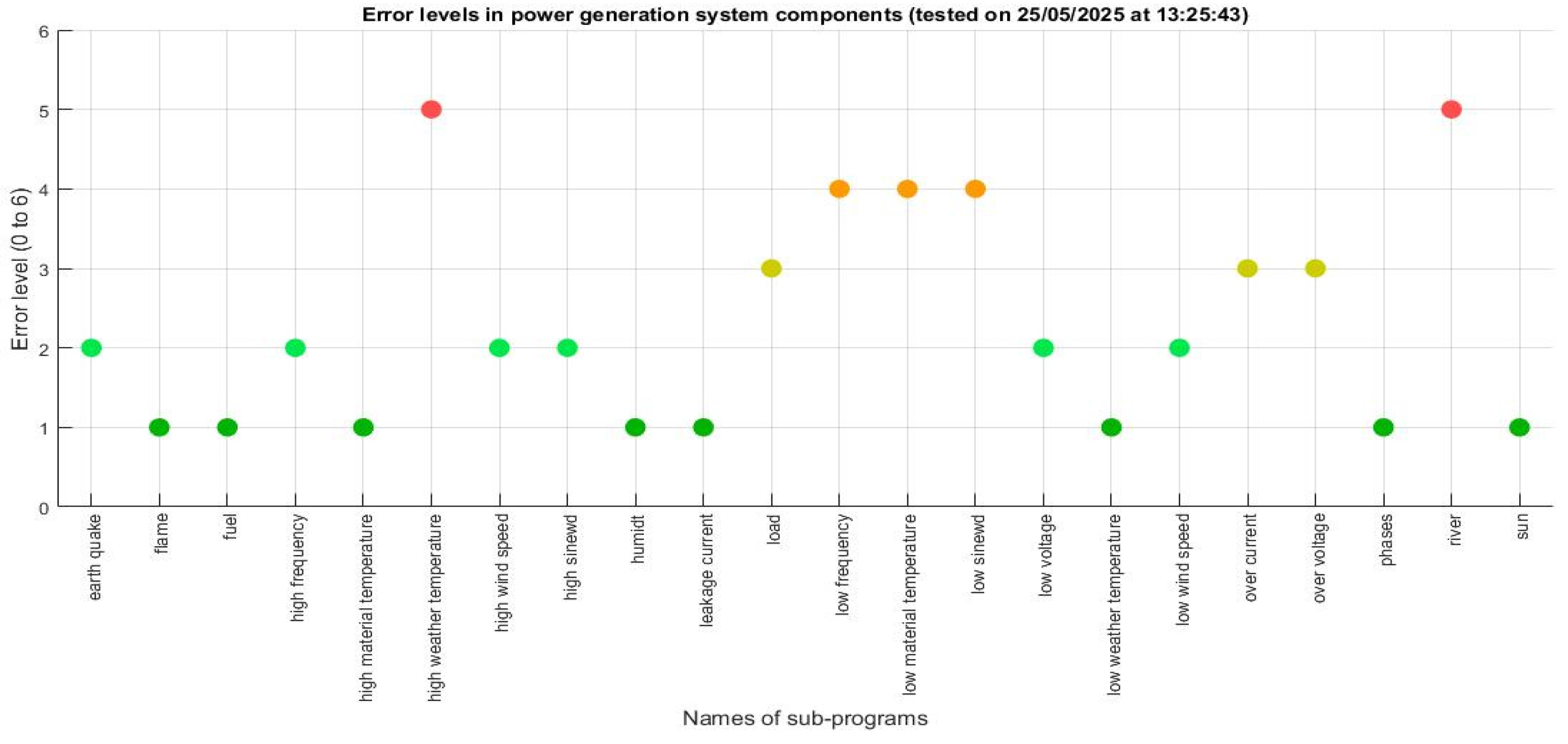
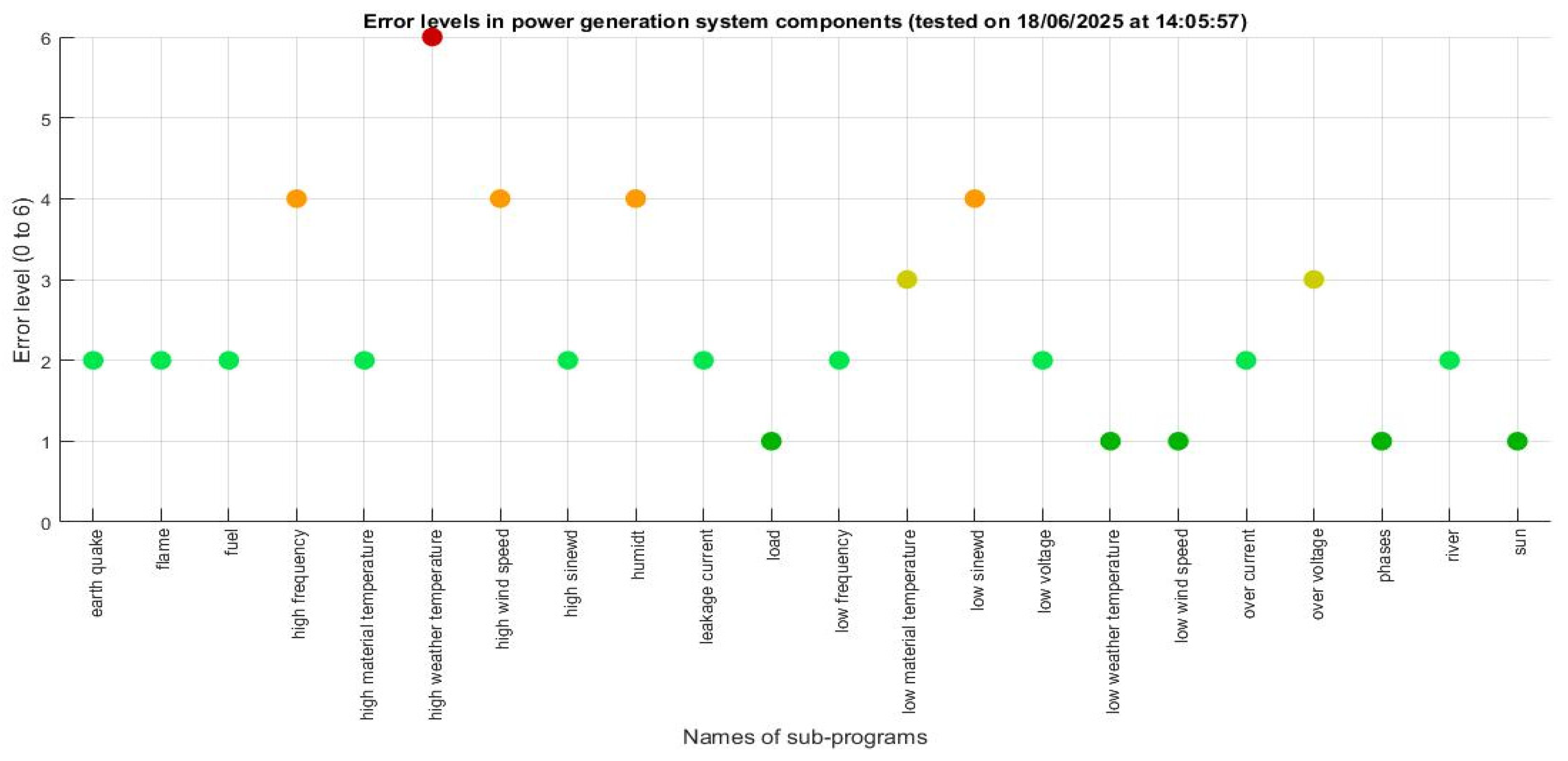
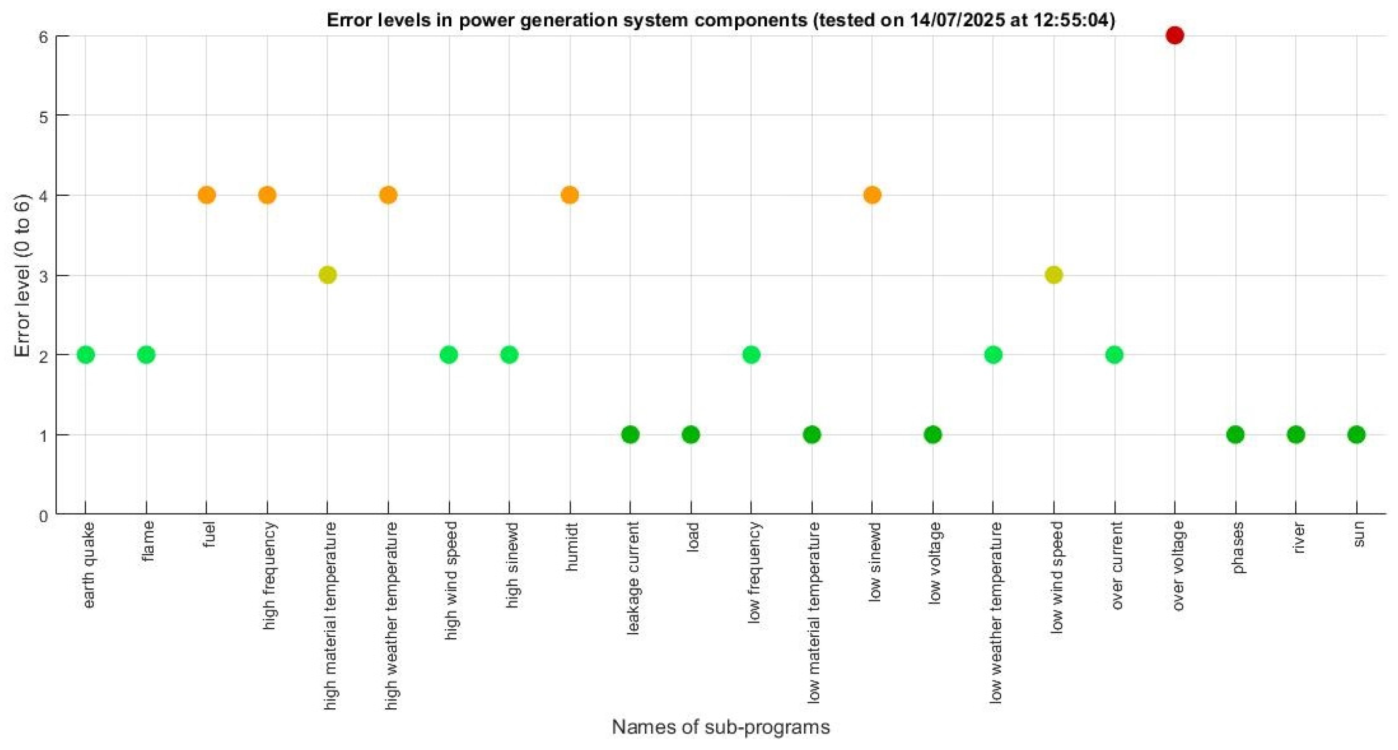
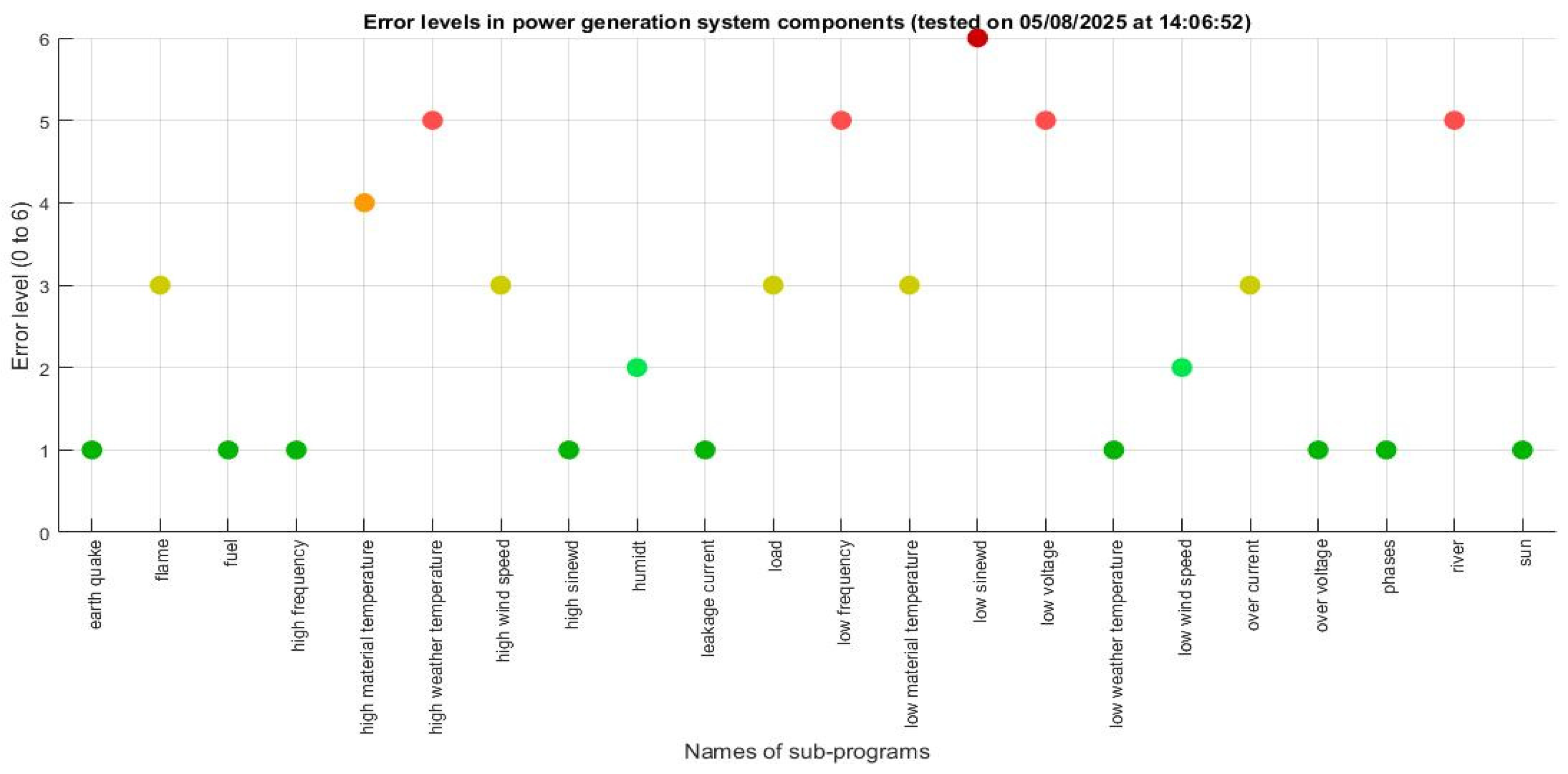
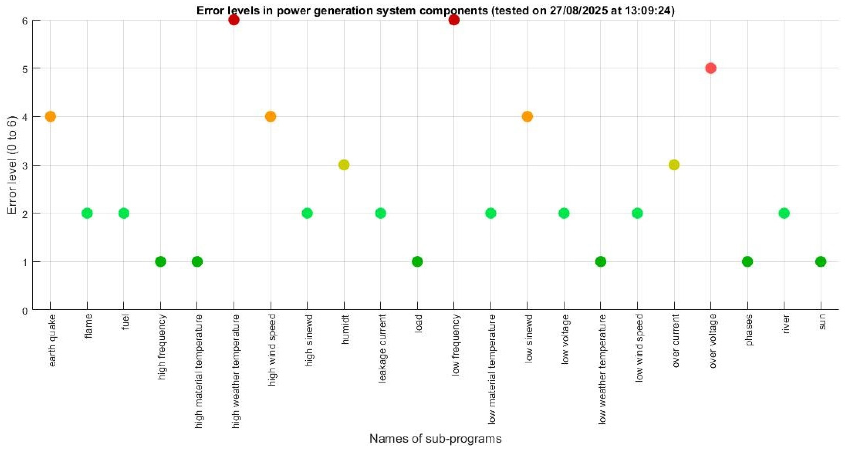
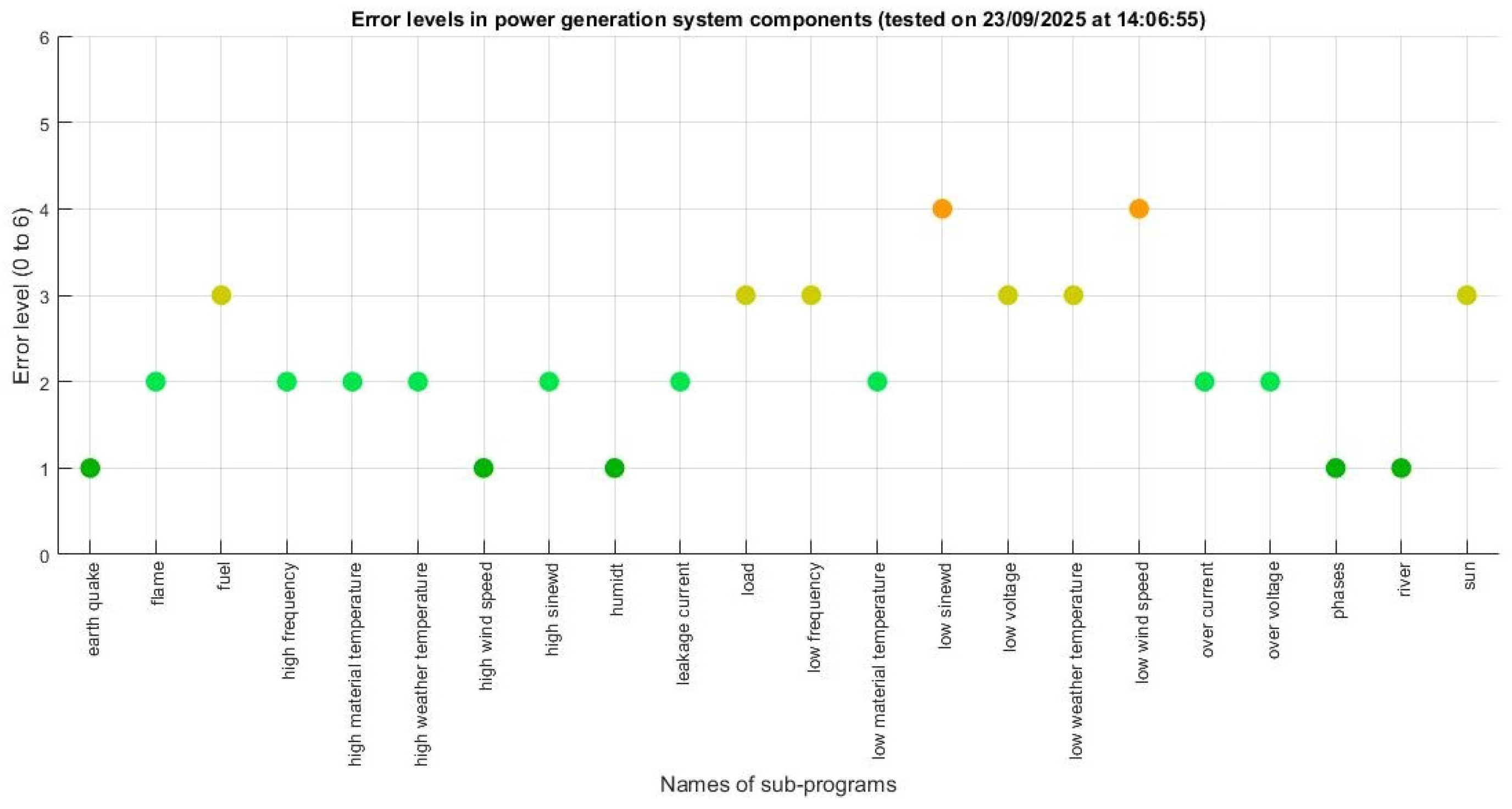
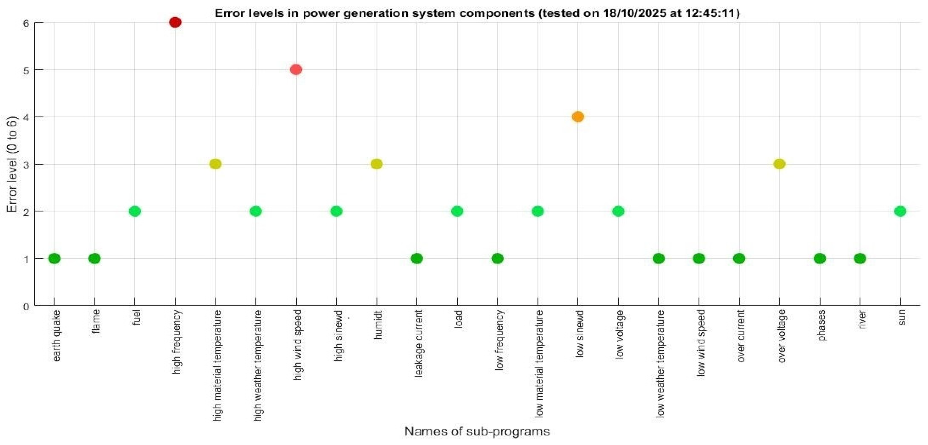
	Time	16:20:24	15:12:45	12:45:55	22:06:36	23:36:15	13:25:43	14:05:57	12:55:04	14:06:52	13:09:24	14:06:55	12:45:11	20:15:34	15:27:13	22:15:27
Earthquake (Richter)		1.5	3.65	2.17	4.77	1.74	2.45	3.22	3.41	0.69	4.63	1.36	0.87	1.28	3.31	1.35
Flame (Photovoltage)		2.75	3.14	1.74	3.96	2.01	2.04	3.24	2.76	4.12	2.73	2.84	1.68	1.98	2.34	1.85
Fuel (Liter)		28	30	31	20	33	28	20	9	29	17	13	20	21	9	19
High frequency (Hz)		50.14	50.06	50.17	50.38	49.91	49.97	50.16	50.13	49.69	49.7	49.82	50.38	49.87	50.16	49.93
High material temperature (°C)		6	8	−10	12	56	−10	7	24	43	−4	17	27	14	4	3
High weather temperature (°C)		8	2	11	12	27	36	39	31	34	39	9	10	14	4	−8
High wind speed (m/s)		18	16	15	18	17	11	18	12	15	18	7	19	10	12	16
High sine wave rate (Vmax/Vef)		0.705	0.719	0.711	0.732	0.721	0.71	0.713	0.693	0.69	0.713	0.702	0.714	0.713	0.69	0.721
Humidity (%)		10	14	15	48	7	12	44	46	21	31	12	33	27	46	15
Leakage current (mA)		8	6	15	12	26	6	15	7	8	13	17	8	4	9	7
Load (A)		55	79	69	83	60	82	63	62	81	55	83	73	71	80	57
Low frequency (Hz)		50.1	50.18	50.17	50.31	49.92	49.83	50.13	50.11	49.73	49.63	49.97	50.33	49.96	50.17	49.92
Low material temperature (°C)		17	8	−19	7	52	−1	12	48	17	33	25	28	12	−15	12
Low sine wave (Vmin/Vef)		0.712	0.721	0.692	0.721	0.719	0.714	0.709	0.71	0.69	0.712	0.713	0.711	0.713	0.69	0.722
Low voltage (V)		228	225	221	219	220	224	225	228	216	225	220	225	217	224	229
Low weather temperature (°C)		13	21	35	12	20	35	30	20	33	28	10	28	29	33	3
Low wind speed		18	13	17	18	13	12	15	8	11	12	6	18	9	8	19
Over current (A)		73	54	67	53	69	66	58	60	68	66	58	50	66	60	71
Over voltage (V)		229	225	221	221	227	225	224	230	217	229	220	224	216	225	229
Phases (Order)		321	123	123	123	123	123	123	123	123	123	123	123	123	123	123
River (m)		13	14	10	16	13	18	14	9	18	13	8	9	15	14	13
Sun (Candela)		70,453	53,879	79,364	0	0	103,215	96,374	94,637	10,841	102,321	52,342	73,174	25,346	39,467	0

according to their physical quantities.

According to the one-year literature-based error generation process, the six-level scoring system obtained for 15 examples is given in

Table 10. Six-level responses for the 15 samples generated over one year according to the reference boundaries and system rules. Dates are given in the DD/MM/YY format (e.g., 19/01/25 denotes 19 January 2025).

Names of Sub-Programs	No	1	2	3	4	5	6	7	8	9	10	11	12	13	14	15
	Date	19/01/25	15/02/25	13/03/25	05/04/25	29/04/25	25/05/25	18/06/25	14/07/25	05/08/25	27/08/25	23/09/25	18/10/25	15/11/25	10/12/25	15/01/26
	Time	16:20:24	15:12:45	12:45:55	22:06:36	23:36:15	13:25:43	14:05:57	12:55:04	14:06:52	13:09:24	14:06:55	12:45:11	20:15:34	15:27:13	22:15:27
Earthquake (Richter)		1	3	2	4	1	2	2	2	1	4	1	1	1	2	1
Flame (Photovoltage)		2	2	1	3	1	1	2	2	3	2	2	1	1	1	1
Fuel (Liter)		1	1	1	2	1	1	2	4	1	2	3	2	2	3	2
High frequency (Hz)		4	3	4	6	2	2	4	4	1	1	2	6	2	4	2
High material temperature (°C)		2	2	1	2	6	1	2	3	4	1	2	3	2	1	2
High weather temperature (°C)		2	1	2	2	4	5	6	4	5	6	2	2	2	1	1
High wind speed (m/s)		4	3	3	4	4	2	4	2	3	4	1	5	2	2	3
High sine wave rate (Vmax/Vef)		2	3	2	4	3	2	2	2	1	2	2	2	2	1	3
Humidity (%)		1	1	1	5	1	1	4	4	2	3	1	3	2	4	1
Leakage current (mA)		1	1	2	2	4	1	2	1	1	2	2	1	1	1	1
Load (A)		1	3	2	3	1	3	1	1	3	1	3	2	2	3	1
Low frequency (Hz)		2	2	2	1	3	4	2	2	5	6	3	1	3	2	3
Low material temperature (°C)		3	3	6	3	1	4	3	1	3	2	2	2	3	5	3
Low sine wave (Vmin/Vef)		4	3	5	3	3	4	4	4	6	4	4	4	4	6	3
Low voltage (V)		1	2	2	3	3	2	2	1	5	2	3	2	4	2	1
Low weather temperature (°C)		3	2	1	3	2	1	1	2	1	1	3	1	1	1	4
Low wind speed		1	2	1	1	2	2	1	3	2	2	4	1	3	3	1
Over current (A)		5	2	3	2	4	3	2	2	3	3	2	1	3	2	5
Over voltage (V)		5	3	2	2	4	3	3	6	1	5	2	2	1	3	5
Phases (Order)		6	1	1	1	1	1	1	1	1	1	1	1	1	1	1
River (m)		2	2	1	3	2	5	2	1	5	2	1	1	3	2	2
Sun (Candela)		5	3	2	6	6	1	1	1	1	1	3	2	5	4	6

.

In the annual evaluation obtained by running 22 subprograms, the number of simultaneous repetitions of the six-level classification for 15 samples is shown in

Table 11. Simultaneous repetition counts of the six-level classification for 15 annual samples. Time stamps are given in the DD/MM/YYYY HH:MM:SS format.

No	Operation Date and Time	Repetition Counts
		Level_1	Level_2	Level_3	Level_4	Level_5	Level_6
1	19/01/2025 16:20:24	7	6	2	3	3	1
2	15/02/2025 15:12:45	5	8	9	0	0	0
3	13/03/2025 12:45:55	8	8	3	1	1	1
4	05/04/2025 22:06:36	3	6	7	3	1	2
5	29/04/2025 23:36:15	7	4	4	5	0	2
6	25/05/2025 13:25:43	8	6	3	3	2	0
7	18/06/2025 14:05:57	5	10	2	4	0	1
8	14/07/2025 12:55:04	7	7	2	5	0	1
9	05/08/2025 14:06:52	9	2	5	1	4	1
10	27/08/2025 13:09:24	6	8	2	3	1	2
11	23/09/2025 14:06:55	5	9	6	2	0	0
12	18/10/2025 12:45:11	9	7	3	1	1	1
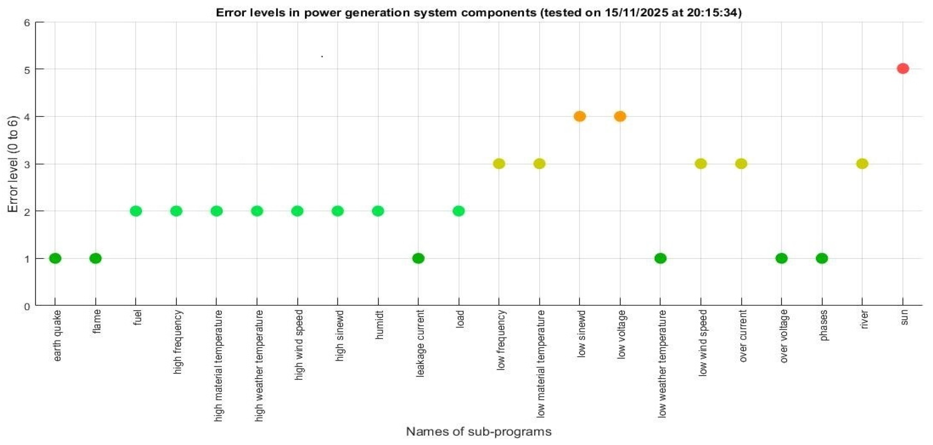
13	15/11/2025 20:15:34	6	8	5	2	1	0
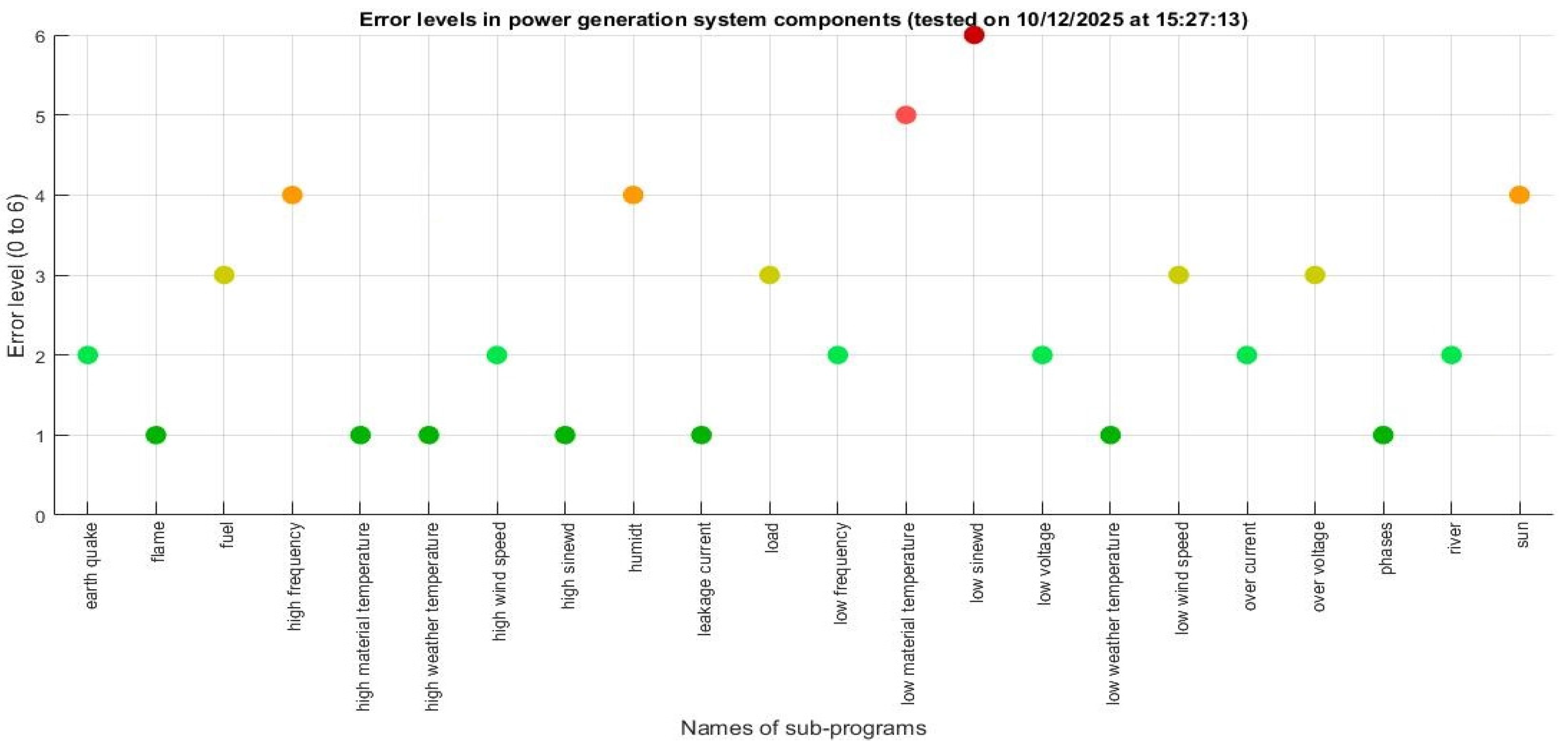
14	10/12/2025 15:27:13	7	6	4	3	1	1
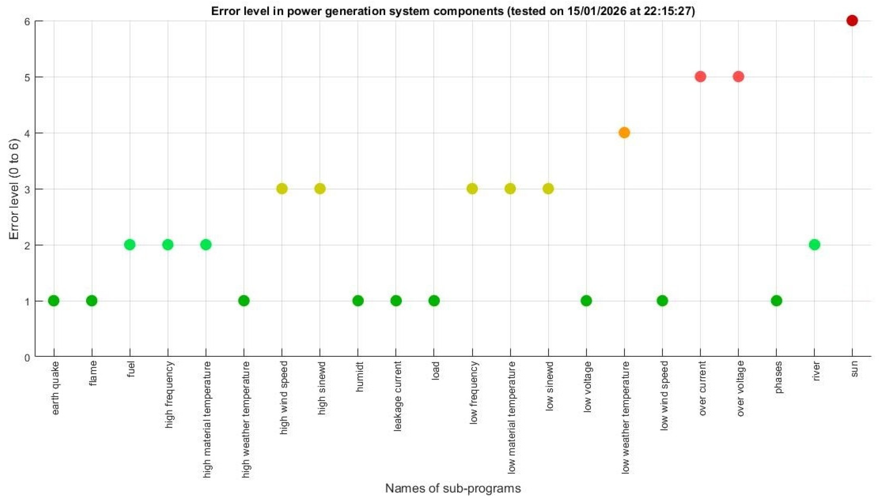
15	15/01/2026 22:15:17	9	4	5	1	2	1

.

The evaluations, which are consistent with the database created as a result of the study and used in the fault analysis of electrical energy systems, are summarized in Table 9, Table 10, Table 11 and

Table 12. Alert-level summary for the one-year evaluation period. Time stamps are given in the DD/MM/YYYY HH:MM:SS format.

Date and Time	Normal Count L1	Warning Counts L2–L4	Critical Counts L5–L6	Program Interpretation
19/01/2025 16:20:24	7	L2 = 6, L3 = 2, L4 = 3	L5 = 3, L6 = 1	Low warnings dominate; one medium alert; no shutdown.
15/02/2025 15:12:45	5	L2 = 8, L3 = 9, L4 = 0	L5 = 0, L6 = 0	Mostly normal/low states; medium alerts and one STOP.
13/03/2025 12:45:55	8	L2 = 8, L3 = 3, L4 = 1	L5 = 1, L6 = 1	Normal and low-warning states dominate; one STOP.
05/04/2025 22:06:36	3	L2 = 6, L3 = 7, L4 = 3	L5 = 1, L6 = 2	Low and medium warnings accumulate; two STOP states.
29/04/2025 23:36:15	7	L2 = 4, L3 = 4, L4 = 5	L5 = 0, L6 = 2	Moderate risk concentration; one STOP state.
25/05/2025 13:25:43	8	L2 = 6, L3 = 3, L4 = 3	L5 = 2, L6 = 0	Mostly normal/low states; medium alerts; no shutdown.
18/06/2025 14:05:57	5	L2 = 10, L3 = 2, L4 = 4	L5 = 0, L6 = 1	Low warnings dominate; one STOP state.
14/07/2025 12:55:04	7	L2 = 7, L3 = 2, L4 = 5	L5 = 0, L6 = 1	Repeated low and level-4 warnings; one STOP state.
05/08/2025 14:06:52	9	L2 = 2, L3 = 5, L4 = 1	L5 = 4, L6 = 1	Normal states with multiple medium alerts and two STOP states.
27/08/2025 13:09:24	6	L2 = 8, L3 = 2, L4 = 3	L5 = 1, L6 = 2	Low/medium warning classes dominate; no shutdown.
23/09/2025 14:06:55	5	L2 = 9, L3 = 6, L4 = 2	L5 = 0, L6 = 0	Low and level-3 warnings dominate; no shutdown.
18/10/2025 12:45:11	9	L2 = 7, L3 = 3, L4 = 1	L5 = 1, L6 = 1	Mostly normal/low states; one STOP state.
15/11/2025 20:15:34	6	L2 = 8, L3 = 5, L4 = 2	L5 = 1, L6 = 0	Low-to-medium risk; one STOP state.
10/12/2025 15:27:13	7	L2 = 6, L3 = 4, L4 = 3	L5 = 1, L6 = 1	Balanced low/medium risk; one STOP state.
15/01/2026 22:15:17	9	L2 = 4, L3 = 5, L4 = 1	L5 = 2, L6 = 1	Low warnings dominate; two STOP states.

. Table 11 shows simultaneous repetition counts of the six-level classification for 15 annual samples. Table 12 shows the number and variety of warning levels that may arise during a one-year evaluation and monitoring period. High-level warning levels caused by chain reactions of abnormal conditions either do not occur or occur only in small numbers under normal conditions. Power deficiencies, lack of maintenance, environmental stress, and incorrect user behavior would negatively affect these results. The geographical region considered here is the northern hemisphere under Tropic of Cancer conditions.

The data presented in these tables illustrate how the developed software processes deviations represented by the different color levels shown in the graphs. Table 9 presents a sample dataset representing measurements that may be obtained from a real-world application. Based on these data, Table 10 shows the corresponding six-level deviation classifications generated by the software. Table 11 summarizes the frequency of occurrence of each deviation level for the 15 representative parameters using 22 input data samples for each parameter. Finally, Table 12 presents the software’s overall evaluation based on the deviation levels and their frequencies of occurrence summarized in Table 11.

When the 15 sample data points obtained for a one-year follow-up are evaluated based on the determination-based data table, the cleaned compact evaluation outputs are obtained. The earlier long case-by-case list was condensed into one row per sample day to prevent table overlap and to make the alert logic readable. These outputs show how database rows are converted into operational warning classes by the software.

In the stages where level 2 and 3 outputs are obtained, generally low-level warning outputs are received, but sometimes high-level warning outputs are obtained, taking into account the repetition counts from the 22 variables. In the stages where level 4 and 5 outputs are obtained, generally high-level warning outputs are received, but sometimes low-level warning outputs are obtained, albeit in small numbers, depending on the repetition counts from the 22 variables. In addition, a high number of repetitions of low-level warning data can, in rare cases, trigger a system disable output. A rare level 6 warning signal requires the system to be deactivated. Whether the entire system or only a part of it needs to be disabled is entirely a design outcome determined by the user.

Since the system has the ability to provide lower-level warning information prior to the shutdown output, users and monitors should take these lower-level warnings into account and make the necessary adjustments. The shutdown stage is avoided when measures are taken to mitigate the effects that hinder the operation of the electrical energy system, such as reducing over currents, activating additional power sources, and ensuring protection against physical damaging factors.

6. Conclusions

This study presented a software-based database-generation and smart-learning-oriented evaluation framework for renewable-integrated electrical energy systems. The main contribution is not limited to fault detection; the proposed software creates a structured, labeled, and reusable database from 22 electrical, thermal, environmental, and resource-related variables when long-term real fault records are not yet available.

The first innovation is the unified treatment of heterogeneous risk factors within a six-level mathematical severity scale. The second innovation is the conversion of literature-based limits and simulated operating states into database rows that include raw inputs, severity outputs, repetition counts, and final alert labels. The third innovation is the use of this database as a training and expansion mechanism for future predictive-maintenance and smart-protection systems.

The software maps the combined severity state of all 22 parameters to a hierarchical three-tier alert scheme as follows: a low-level advisory alert (“warning”), a medium-level operational warning (“WARNING!”), and a high-level shutdown command (“STOP”). Because intermediate warning levels are produced before shutdown, the framework supports preventive action rather than only post-fault isolation.

Overall, the proposed approach fills a practical gap between conventional protection logic and data-driven learning systems. It provides an initial database when real records are scarce, explains how new records are generated and appended, and creates a transparent mathematical basis for classifying system risk. Future work should validate the generated database against real telemetry data, optimize weighting coefficients for different network types, and integrate the database with machine-learning models for real-time fault prediction.

It should be emphasized that the contribution of this work is not the simulation of data in isolation, but the complete and reproducible workflow that links the following four stages within a single framework: (i) standards- and literature-grounded definition of variable limits, (ii) mathematical severity normalization of 22 heterogeneous electrical, thermal, environmental, and resource-related factors onto a common six-level scale, (iii) priority-weighted aggregation into a global risk index with multi-level alert labeling, and (iv) the automatic construction of a structured, labeled, and expandable database. Cross-variable normalization is indeed a common preprocessing step; here, it is not presented as the contribution in itself, but as one stage of this coupled pipeline that turns raw operating states into decision-ready, learning-ready records. Regarding data validity, the synthetic records are not arbitrary: their limits, occurrence frequencies, and severity weights are anchored to the measured determination data summarized in Table 4 and to published protection thresholds, so they reproduce realistic operating and fault patterns rather than random values. The framework is therefore intended as a bootstrap training resource for situations in which long-term real fault records are scarce or unsafe to reproduce, and the database schema is explicitly designed so that field telemetry, once available, can be appended to and used to refine the generated rows and the decision boundaries. Finally, the “smart-learning” designation reflects this role directly: the software produces the labeled input–output pairs, severity sequences, and alert classes that constitute the training substrate and the rule base on which predictive-maintenance and intelligent-protection models are subsequently learned, so the title is consistent with the scope of the work.

Future research will focus on three directions. First, the framework will be validated against real-time telemetry data from operational substations and renewable generation facilities, enabling a quantitative comparison between simulation-derived and empirically observed fault frequencies. Second, the generated database will be used to train and evaluate a suite of machine learning architectures—including gradient-boosted decision trees, convolutional neural networks applied to temporal severity sequences, and hybrid attention-based models—to determine which approaches best generalize across unseen fault scenarios. Third, the parameter set will be expanded to capture emerging fault modes associated with large-scale battery energy storage systems, power-electronics-dense microgrids, and vehicle-to-grid interfaces, reflecting the evolving composition of modern electrical infrastructure. These extensions are expected to further consolidate the role of data-driven, multi-parameter risk assessment as a cornerstone of next-generation power system protection and maintenance strategies.

References

- Ahmed, M.M.R.; Mirsaeidi, S.; Koondhar, M.A.; Karami, N.; Tag-Eldin, E.M.; Ghamry, N.A.; Sharaf, A.M. Mitigating Uncertainty Problems of Renewable Energy Resources Through Efficient Integration of Hybrid Solar PV/Wind Systems into Power Networks. IEEE Access 2024, 12, 30311–30328. [Google Scholar] [CrossRef] [Scilit]
- Etukudoh, E.A.; Fabuyide, A.; Ibekwe, K.I.; Sonko, S.; Ilojianya, V.I. Electrical engineering in renewable energy systems: A review of design and integration challenges. Eng. Sci. Technol. J. 2024, 5, 231–244. [Google Scholar] [CrossRef] [Scilit]
- Liu, S.; Yang, N.; Song, X.; Liu, X.; Jiang, Q. Real-time scheduling of renewable power systems through planning-based reinforcement learning. In Proceedings of the 2025 IEEE PES Innovative Smart Grid Technologies-Asia (ISGT Asia), Valletta, Malta, 20–23 October 2025; pp. 60–66. [Google Scholar]
- Safder, M.U.; Sanjari, M.J.; Hamza, A.; Garmabdari, R.; Hossain, M.A.; Lu, J. Enhancing microgrid stability and energy management: Techniques, challenges, and future directions. Energies 2023, 16, 6417. [Google Scholar] [CrossRef] [Scilit]
- Saxena, A.; Shankar, R.; El-Saadany, E.; Kumar, M.; Al Zaabi, O.; Al Hosani, K.; Muduli, U.R. Intelligent load forecasting and renewable energy integration for enhanced grid reliability. IEEE Trans. Ind. Appl. 2024, 60, 8403–8417. [Google Scholar] [CrossRef] [Scilit]
- Stoliarov, O. Efficient electricity generation forecasting from solar power plants using technology: Integration, benefits and prospects. Bull. Cherkasy State Technol. Univ. Tech. Sci. 2024, 29, 73–85. [Google Scholar] [CrossRef] [Scilit]
- Veeramachaneni, V. Optimizing renewable energy integration in AI-driven data centers using quantum algorithms. J. Netw. Secur. Data Min. 2025, 8, 36–48. [Google Scholar]
- Aghdam, F.H.; Mohammadi-Ivatloo, B.; Abapour, M.; Marzband, M.; Rasti, M.; Pongracz, E. Enhancing the risk-oriented participation of wind power plants in day-ahead, balancing, and hydrogen markets with shared multi-energy storage systems. J. Energy Storage 2025, 107, 114911. [Google Scholar] [CrossRef] [Scilit]
- Jargalsaikhan, N.; Ueda, S.; Masahiro, F.; Matayoshi, H.; Mikhaylov, A.; Byambaa, S.; Senjyu, T. Exploring the influence of air density deviation on power production of wind energy conversion system: Study on correction method. Renew. Energy 2024, 220, 119636. [Google Scholar] [CrossRef] [Scilit]
- Pata, S.K.; Pata, U.K. Comparative analysis of the impacts of solar, wind, biofuels and hydropower on load capacity factor and sustainable development index. Energy 2025, 319, 134991. [Google Scholar] [CrossRef] [Scilit]
- Shaabani, B.; Chatoorgoon, V.; Bibeau, E.L. Using numerical analysis to design and optimize river hydrokinetic turbines’ capacity factor to address seasonal velocity variations. Energies 2025, 18, 477. [Google Scholar] [CrossRef] [Scilit]
- Van Dijk, M.; Gezer, D.; Rudolf, P. Unlocking hydropower’s potential: Retrofitting infrastructure and harnessing unconventional sources for clean energy transitions. In IOP Conference Series: Earth and Environmental Science; IOP Publishing: Bristol, UK, 2025; Volume 1442, p. 012006. [Google Scholar]
- Wang, Y.; Levin, T.; Kwon, J.; Baker, E. The value of hydropower flexibility for electricity system decarbonization. Energy Rep. 2025, 13, 2711–2721. [Google Scholar] [CrossRef] [Scilit]
- Allal, Z.; Noura, H.N.; Salman, O.; Chahine, K. Machine learning solutions for renewable energy systems: Applications, challenges, limitations, and future directions. J. Environ. Manag. 2024, 354, 120392. [Google Scholar] [CrossRef] [Scilit] [PubMed]
- Allal, Z.; Noura, H.N.; Vernier, F.; Salman, O.; Chahine, K. Wind turbine fault detection and identification using a two-tier machine learning framework. Intell. Syst. Appl. 2024, 22, 200372. [Google Scholar] [CrossRef] [Scilit]
- Cao, H.; Zhang, D.; Yi, S. Real-time machine learning-based fault detection, classification, and location in large scale solar energy-based systems: Digital twin simulation. Sol. Energy 2023, 251, 77–85. [Google Scholar] [CrossRef] [Scilit]
- Ding, X.; Gong, Y.; Wang, C.; Zheng, Z. Artificial intelligence based abnormal detection system and method for wind power equipment. Int. J. Thermofluids 2024, 21, 100569. [Google Scholar] [CrossRef] [Scilit]
- Elshenawy, L.M.; Gafar, A.A.; Awad, H.A.; AbouOmar, M.S. Fault detection of wind turbine system based on data-driven methods: A comparative study. Neural Comput. Appl. 2024, 36, 10279–10296. [Google Scholar] [CrossRef] [Scilit]
- Furse, C.M.; Kafal, M.; Razzaghi, R.; Shin, Y.J. Fault diagnosis for electrical systems and power networks: A review. IEEE Sens. J. 2021, 21, 888–906. [Google Scholar] [CrossRef] [Scilit]
- Jove, E.; González-Cava, J.M.; Casteleiro-Roca, J.L.; Alaiz-Moretón, H.; Baruque, B.; Leitão, P.; Calvo-Rolle, J.L. An intelligent system for harmonic distortions detection in wind generator power electronic devices. Neurocomputing 2021, 456, 609–621. [Google Scholar] [CrossRef] [Scilit]
- Moloi, K.; Hamam, Y.; Jordaan, J.A. A support vector machine based technique for fault detection in a power distribution integrated system with renewable energy distributed generation. Adv. Sci. Technol. Eng. Syst. J. 2020, 5, 577–588. [Google Scholar] [CrossRef] [Scilit]
- Ozcanli, A.K.; Yaprakdal, F.; Baysal, M. Deep learning methods and applications for electrical power systems: A comprehensive review. Int. J. Energy Res. 2020, 44, 7136–7157. [Google Scholar] [CrossRef] [Scilit]
- Panigrahi, B.K.; Bhuyan, A.; Shukla, J.; Ray, P.K.; Pati, S. A comprehensive review on intelligent islanding detection techniques for renewable energy integrated power system. Int. J. Energy Res. 2021, 45, 14085–14116. [Google Scholar] [CrossRef] [Scilit]
- Anwar, T.; Mu, C.; Yousaf, M.Z.; Khan, W.; Khalid, S.; Hourani, A.O.; Zaitsev, I. Robust fault detection and classification in power transmission lines via ensemble machine learning models. Sci. Rep. 2025, 15, 2549. [Google Scholar] [CrossRef] [Scilit] [PubMed]
- Ibrahim, M.S.; Dong, W.; Yang, Q. Machine learning driven smart electric power systems: Current trends and new perspectives. Appl. Energy 2020, 272, 115237. [Google Scholar] [CrossRef] [Scilit]
- Kaitouni, S.I.; Abdelmoula, I.A.; Es-sakali, N.; Mghazli, M.O.; Er-retby, H.; Zoubir, Z.; Brigui, J. Implementing a digital twin-based fault detection and diagnosis approach for optimal operation and maintenance of urban distributed solar photovoltaics. Renew. Energy Focus 2024, 48, 100530. [Google Scholar] [CrossRef] [Scilit]
- Najafzadeh, M.; Pouladi, J.; Daghigh, A.; Beiza, J.; Abedinzade, T. Fault detection, classification and localization along the power grid line using optimized machine learning algorithms. Int. J. Comput. Intell. Syst. 2024, 17, 49. [Google Scholar] [CrossRef] [Scilit]
- Pujara, D.; Ramirez, D.; Tepedelenlioglu, C.; Srinivasan, D.; Spanias, A. Real-time PV fault detection using embedded machine learning. In Proceedings of the 2024 IEEE 7th International Conference on Industrial Cyber-Physical Systems (ICPS); IEEE: New York, NY, USA, 2024; pp. 1–5. [Google Scholar]
- Satyanrayana, M.; Veeramsetty, V.; Rajababu, D. Signal processing approaches for power quality disturbance classification: A comprehensive review. Results Eng. 2025, 25, 104569. [Google Scholar] [CrossRef] [Scilit]
- Bo, Z.Q.; Lin, X.N.; Wang, Q.P.; Yi, Y.H.; Zhou, F.Q. Developments of power system protection and control. Prot. Control Mod. Power Syst. 2016, 1, 7. [Google Scholar] [CrossRef] [Scilit]
- Boza, P.; Evgeniou, T. Artificial intelligence to support the integration of variable renewable energy sources to the power system. Appl. Energy 2021, 290, 116754. [Google Scholar] [CrossRef] [Scilit]
- Nascimento, J.P.; Brito, N.S.; Souza, B.A. An adaptive overcurrent protection system applied to distribution systems. Comput. Electr. Eng. 2020, 81, 106545. [Google Scholar] [CrossRef] [Scilit]
- Feng, X.; Xiong, Q.; Wardell, D.; Gattozzi, A.L.; Strank, S.M.; Hebner, R.E. Extra-fast DC distribution system protection for future energy systems. IEEE Trans. Ind. Appl. 2019, 55, 3421–3430. [Google Scholar] [CrossRef] [Scilit]
- Kumar, S.; Saket, R.K.; Dheer, D.K.; Holm-Nielsen, J.B.; Sanjeevikumar, P. Reliability enhancement of electrical power system including impacts of renewable energy sources: A comprehensive review. IET Gener. Transm. Distrib. 2020, 14, 1799–1815. [Google Scholar] [CrossRef] [Scilit]
- Tovar-Facio, J.; Martín, M.; Ponce-Ortega, J.M. Sustainable energy transition: Modeling and optimization. Curr. Opin. Chem. Eng. 2021, 31, 100661. [Google Scholar] [CrossRef] [Scilit]
- Koohi-Fayegh, S.; Rosen, M.A. A review of renewable energy options, applications, facilitating technologies and recent developments. Eur. J. Sustain. Dev. Res. 2020, 4, em0138. [Google Scholar] [CrossRef] [Scilit] [PubMed]
- Liu, Y.; Ning, P.; Reiter, M.K. False data injection attacks against state estimation in electric power grids. ACM Trans. Inf. Syst. Secur. 2011, 14, 1–33. [Google Scholar] [CrossRef] [Scilit]
- Salem, A.A.; Abd-Rahman, R.; Al-Gailani, S.A.; Kamarudin, M.S.; Ahmad, H.; Salam, Z. The leakage current components as a diagnostic tool to estimate contamination level on high voltage insulators. IEEE Access 2020, 8, 92514–92528. [Google Scholar] [CrossRef] [Scilit]
- Erdiwansyah, F.; Mahidin, F.; Husin, H.; Nasaruddin, F.; Zaki, M.; Muhibbuddin, F. A critical review of the integration of renewable energy sources with various technologies. Prot. Control Mod. Power Syst. 2021, 6, 3. [Google Scholar] [CrossRef] [Scilit]
- Mathiesen, B.V.; Lund, H.; Connolly, D.; Wenzel, H.; Østergaard, P.A.; Möller, B.; Hvelplund, F.K. Smart energy systems for coherent 100% renewable energy and transport solutions. Appl. Energy 2015, 145, 139–154. [Google Scholar] [CrossRef] [Scilit]
- IEC 61400-1; Wind Energy Generation Systems—Part 1: Design Requirements. International Electrotechnical Commission: Geneva, Switzerland, 2019.