Input-Adaptive Dynamic Convolution-Augmented Transformer for Energy Demand Forecasting

Abstract

Energy demand forecasting is a critical task in sustainable energy systems, where nonlinearities, temporal dynamics, and multivariate factors pose significant challenges. Despite the success of deep learning methods, how to design and optimize deep learning algorithms is yet to be investigated for energy demand forecasting. To address these issues, we propose an input-adaptive dynamic convolution-augmented Transformer. Specifically, channel, phase, and joint channel–phase embeddings are designed to enrich feature representations. Then, a dynamic convolution module is developed to adaptively learn one-dimensional kernels via input-dependent adaptive attention. The resulting features are further fed into a Transformer encoder for forecasting energy demand. Finally, an efficient Bayesian optimization algorithm is used to automatically design and optimize the proposed method. Experimental results on real-world energy demand forecasting task demonstrate the effectiveness and practicality of the proposed method.

1. Introduction

Accurate energy demand forecasting is a fundamental component of modern power system operations [1,2,3,4]. It underpins grid stability, generation scheduling, transmission planning, and energy market clearing [5,6,7]. In an era of increasing renewable energy penetration and growing demand-side flexibility, precise and reliable load predictions have never been more critical [8,9,10]. Errors in forecasting can lead to either costly over-generation, supply shortages, or blackouts. Hence, substantial research efforts have been devoted to developing sophisticated forecasting models that can capture the complex, nonlinear, and time-varying characteristics of energy consumption [11,12].

Energy demand time series are inherently challenging to predict due to multiple intertwined factors [13]. These include weather conditions, calendar effects, socio-economic variables, and random behavioral patterns of consumers [14,15]. Moreover, the growing integration of distributed energy resources introduces additional volatility and uncertainty [16]. Traditional statistical methods and machine learning ones have been widely applied to load forecasting [1,17]. While computationally efficient, these approaches often struggle to capture the high-dimensional nonlinearities and long-term dependencies present in modern energy demand data [13]. As alternative solutions, deep learning techniques have become the dominant paradigm in energy demand forecasting [4,18]. For example, long short-term memory, and gated recurrent units excel at modeling sequential dependencies [2,19]. Convolutional neural networks and graph neural networks, on the other hand, are adept at extracting local patterns and hierarchical features from time series [14,20,21,22]. As for attention mechanisms and Transformer models, they have also demonstrated promising prospect for energy demand forecasting [10,23,24].

Despite these advances, several challenges remain [13,25]. (1) The temporal patterns in energy demand often exhibit dynamic or multi-scale periodicities (daily, weekly, or seasonal) that require adaptive feature extraction [13,15]. To address these problems, many related studies have been conducted. For example, ensemble learning has been investigated to integrate multiple models with complementary strengths [6,17]. Multi-scale feature decomposition and hybrid algorithm designs have also been explored [14,26,27]. Furthermore, network architectures with multi-scale learning capabilities have been developed [28,29,30]. These methods have been successfully applied to energy-related forecasting problems with complex dynamics. However, they primarily focus on feature extraction algorithms and network architecture design. Although effective, such approaches require careful algorithm design and introduce a large number of learnable parameters, thereby increasing the learning difficulty. Hence, we aim to explore how the intrinsic properties of data can be leveraged to improve algorithmic performance without complex algorithm design. (2) Many existing deep learning models rely on fixed-kernel convolutions [4,21], which may not fully adapt to the varying spatial dynamics of the given data. Some targeted solutions have been proposed, such as multi-scale convolutions with different kernel sizes [18,30] and multi-sight convolutions based on multi-scale decomposition [14]. However, these methods still essentially rely on static convolutions, and cannot adaptively adjust parameters according to different inputs. Although dynamic convolution can effectively solve this problem, it is mainly applied to image-related tasks [31,32,33]. Some studies have also applied dynamic convolution to time-series analysis [34,35]. However, the application of dynamic convolution in energy demand forecasting is yet to be explored. (3) The hyperparameter configuration of a deep learning algorithm has a profound impact on the algorithmic performance, yet manual tuning is labor-intensive and often suboptimal [1,36]. Hence, it is worth investigating how to design and optimize deep learning algorithms for energy demand forecasting.

To address the aforementioned challenges, we propose an input-adaptive dynamic convolution-augmented Transformer, where Bayesian optimization is used to achieve adaptive design. Specifically, we introduce channel, phase, and joint channel–phase embeddings to capture latent periodicities and enrich the feature representation. Moreover, we design an input-adaptive dynamic one-dimensional convolution and integrate it with Transformer, thus enabling flexible feature extraction that adapts to varying energy-related patterns. Finally, we adopt the Tree-Structured Parzen Estimator (TPE) [37] to adaptively design and optimize our method. Two real-world energy demand forecasting tasks are used to investigate the effectiveness of our method.

As an application-oriented study, our main contribution is to develop an automatically optimized hybrid architecture that integrates input-adaptive dynamic convolution with Transformer for energy demand forecasting. Compared with existing complex feature extraction algorithms [14,26,27,38], our embedding strategy can capture the latent periodicity within the data and the spatial relationships among variables without complex algorithm design. Compared with existing convolution–Transformer hybrid methods [18,30], our method improves both the convolutional computation and the hyperparameter optimization strategy. Our method enables input-dependent adaptive convolution and automated parameter optimization. It has been successfully applied to two real-world energy demand forecasting cases.

The rest of our work is organized as follows. Section 2 reviews related work. Section 3 describes the proposed methodology. Section 4 presents the experiments and results. Section 5 concludes with a discussion and future research directions.

2. Related Work

Energy demand forecasting research has evolved into several distinct methodological categories [13,18,39]. These include traditional statistical methods, classical machine learning approaches, deep learning architectures, and hybrid models that blend multiple paradigms. Here, we primarily review the existing literature from two perspectives, including traditional machine learning and deep learning.

The traditional machine learning methods typically rely on feature engineering to capture relationships between demand and influencing factors like weather, time, and economic indicators. For example, Elmrini et al. developed an optimized XGBoost model for high-fidelity load forecasting in rural hybrid energy systems, demonstrating its effectiveness [1]. Gao et al. used a random forest model to forecast the demand function of air conditioning resources in response to energy prices [7]. A hybrid approach combining Light Gradient Boosting Machine (LightGBM) with an LSTM network was designed for high-fidelity forecasting of load demand and electricity prices [40]. Moreover, Bouyakhsaine et al. utilized a LightGBM model within an adaptive online learning framework to predict residential energy consumption, effectively handling concept drift [36]. Tu et al. introduced an arithmetic optimization algorithm to adaptively optimize parameters in a mixed-frequency fractional derivative grey model [41]. While powerful, these models require feature selection and may not inherently capture long-range temporal dependencies as effectively as deep learning methods.

Deep learning methods have become the dominant approach for energy demand forecasting due to their automatic feature extraction and exceptional ability to model nonlinear and long-term temporal dependencies [6,7,13]. For instance, Uhrig et al. proposed a multivariate LSTM-based model that effectively learns complex nonlinear dependencies from heterogeneous inputs for short-term forecasting [2]. Somasundaram and Jothinathan developed a hybrid framework using a deep walk GRU with an attention mechanism for high-resolution peak-load forecasting [42]. Du et al. used a two-layer decomposition framework with CEEMDAN and feature mode decomposition, and combined it with a hybrid architecture of bidirectional TCN, GRU, and attention mechanisms for battery swapping station demand forecasting [43]. Zhu et al. proposed a hybrid strategy combining Mamba for long-term trends and Transformer for short-term fluctuations [24]. Kaur et al. integrated an explainable AI tool with a Transformer-based LSTM model to interpret the influence of weather parameters on residential energy demand [44]. Guo et al. combined a bidirectional LSTM with an attention mechanism and an improved whale optimization algorithm to forecast high-dynamic-load periods [17].

In summary, while numerous deep learning-based methods have been proposed for energy demand forecasting, the practical application environment remains complex due to the highly nonlinear and multi-scale nature of load data. Furthermore, the performance of the advanced models is highly sensitive to hyperparameter settings, and manual tuning or grid search is often inefficient and suboptimal. Hence, how to design efficient algorithms, and how to optimize their numerous hyperparameters in an automated manner, remains an ongoing area of study and worthy of further investigation.

3. Proposed Method

3.1. Overview

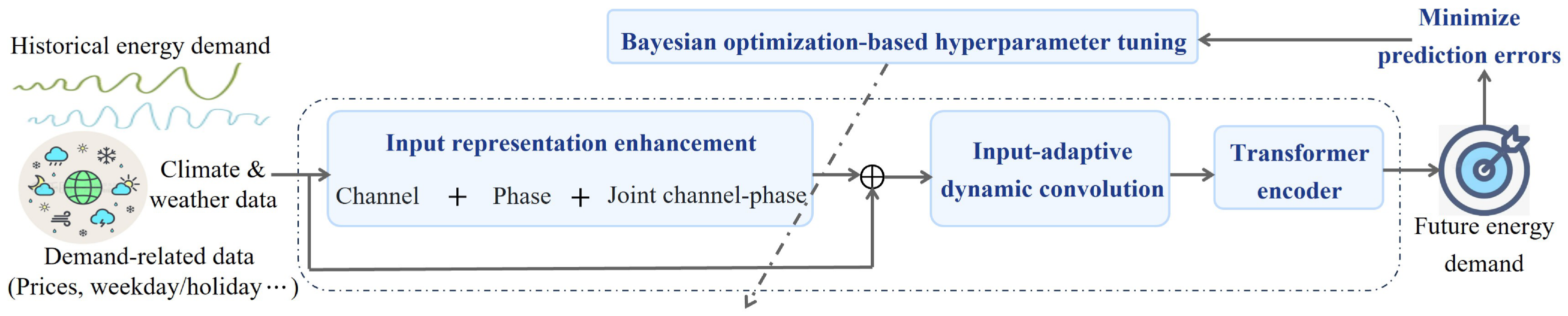
As shown in Figure 1, the proposed method enhances Transformer by redesigning its input representation and feature extraction pathways. On one hand, triple embeddings are introduced to capture channel-wise, phase-wise, and channel–phase joint embeddings from the energy-related data, thus enhancing feature representations. On the other hand, an input-adaptive dynamic convolution is developed to replace the traditional static convolution, thereby improving Transformer’s capacity to extract complex features from given data. Moreover, we introduce an efficient Bayesian optimization algorithm to adaptively design and optimize our method.

Specifically, the input sequence first passes through the channel, phase, and joint embedding branches. The resulting representations are summed with a linear projection of the input and fed into the input-adaptive dynamic convolution module. Subsequently, the dynamic convolution learns the kernel parameters from different inputs, thus achieving convolution computation that adapts to dynamic changes. The output is then added with a learnable positional encoding and processed by a multi-layer Transformer encoder. Finally, Bayesian optimization is employed to automatically design and tune the critical hyperparameters of our method, thus realizing energy demand forecasting. The technical details of our method can be illustrated as follows.

3.2. Channel and Phase Joint Embedding Strategy

To equip the forecasting model with rich inductive biases that capture both inter-channel relationships and temporal periodicity, we introduce a joint embedding strategy that integrates three complementary representations: channel-specific embeddings, phase-aware embeddings, and channel–phase interactions. The core idea is to construct a comprehensive token representation by summing these different components. This design explicitly expresses channel correlations, encodes cyclical phase information, and models the entangled dependencies between channels and time phases. The overall embedding process is illustrated below.

Given the input data $X\in {\mathbb{R}}^{L\times C}$ comprising L historical time steps and C channels (variates), we first apply a learnable linear transformation to project each channel’s time series into a $d_1$-dimensional latent space. Following the variate tokenization paradigm, each channel is represented as a single token. The obtained base token embedding for each channel $H_{\mathrm{base}}$ can be formulated as follows:

$$H_{\mathrm{base}}=X^{\top }{W}_x+b_x\in {\mathbb{R}}^{C\times d_1},$$

(1)

where $W_x\in {\mathbb{R}}^{L\times d_1}$ and $b_x\in {\mathbb{R}}^{d_1}$ are learnable parameters.

To effectively express local inter-channel correlations, we introduce a channel embedding that assigns a unique, time-invariant vector to each channel. This embedding can act as a global identifier, and help the model maintain stable relationships across channels and time steps regardless of fluctuations [45]. We use a learnable lookup table ${\mathsf{\Phi }}_c\in {\mathbb{R}}^{C\times d_1}$, each row of which corresponds to the embedding of one channel. We further broadcast this embedding to all C channels. The final channel embedding for all channels is expressed as follows.

$$H_c=\mathrm{Lookup}({\mathsf{\Phi }}_c,i)\in {\mathbb{R}}^{C\times d_1},$$

(2)

where $\mathrm{Lookup}(·)$ denotes a lookup operation that retrieves the row vector for each channel index $i\in \{1,2,\cdots ,C\}$.

As for the energy consumption data, its temporal patterns often exhibit periodicity. However, both $H_{\mathrm{base}}$ and $H_c$ lack explicit phase information. To encode the position within each periodic cycle and learn phase-dependent patterns, we also introduce a phase embedding that depends on the timestamp of the last observed step. Let P be the predefined period length (e.g., daily or weekly cycles). For a given observation window ending at absolute time t, the phase index is computed as $r=tmodP$. We can construct a learnable embedding matrix ${\mathsf{\Phi }}_p\in {\mathbb{R}}^{P\times d_1}$, where each row corresponds to a specific phase. The corresponding phase embedding is then shared across all channels for the same phase index. Additionally, to align with the token dimension, we broadcast this vector to all C channels, thus obtaining the final phase embedding $H_p$.

$$H_p=\mathrm{Lookup}({\mathsf{\Phi }}_p,r)\in {\mathbb{R}}^{C\times d_1}.$$

(3)

While channel embedding provides stability across time and phase embedding captures periodicity across channels, neither models the intricate interactions between a specific channel and its current phase. For instance, different sensors may exhibit distinct responses at the same phase of a cycle (e.g., morning peak in energy consumption versus solar generation). To capture such cross-axis specificity and disentangle channel-specific temporal characteristics, we introduce a joint embedding that combines channel identity and phase information. Here, we also use a learnable tensor ${\mathsf{\Phi }}_{cp}\in {\mathbb{R}}^{C\times P\times d_1}$, where each entry ${\mathsf{\Phi }}_{cp}[i,r,:]$ is a $d_1$-dimensional vector associated with channel i and phase r. For each channel i and the current phase r, we retrieve the corresponding joint embedding. By stacking all channels, we can then obtain the full joint embedding matrix $H_{cp}$. As a result, this embedding enables the model to learn fine-grained patterns where each channel’s periodic dynamics are encoded uniquely. $H_{cp}$ is formulated as follows.

$$H_{cp}=\mathrm{Lookup}({\mathsf{\Phi }}_{cp},i,r)\in {\mathbb{R}}^{C\times d_1}.$$

(4)

Finally, we fuse the four components by element-wise summation to form the input token representation for subsequent layers. This combined embedding simultaneously encodes raw temporal projections, stable channel identities, global phase information, and channel-phase interactions.

$$U_0=H_{\mathrm{base}}+H_c+H_p+H_{cp}\in {\mathbb{R}}^{C\times d_1}.$$

(5)

3.3. Input-Adaptive Dynamic Convolution-Augmented Transformer

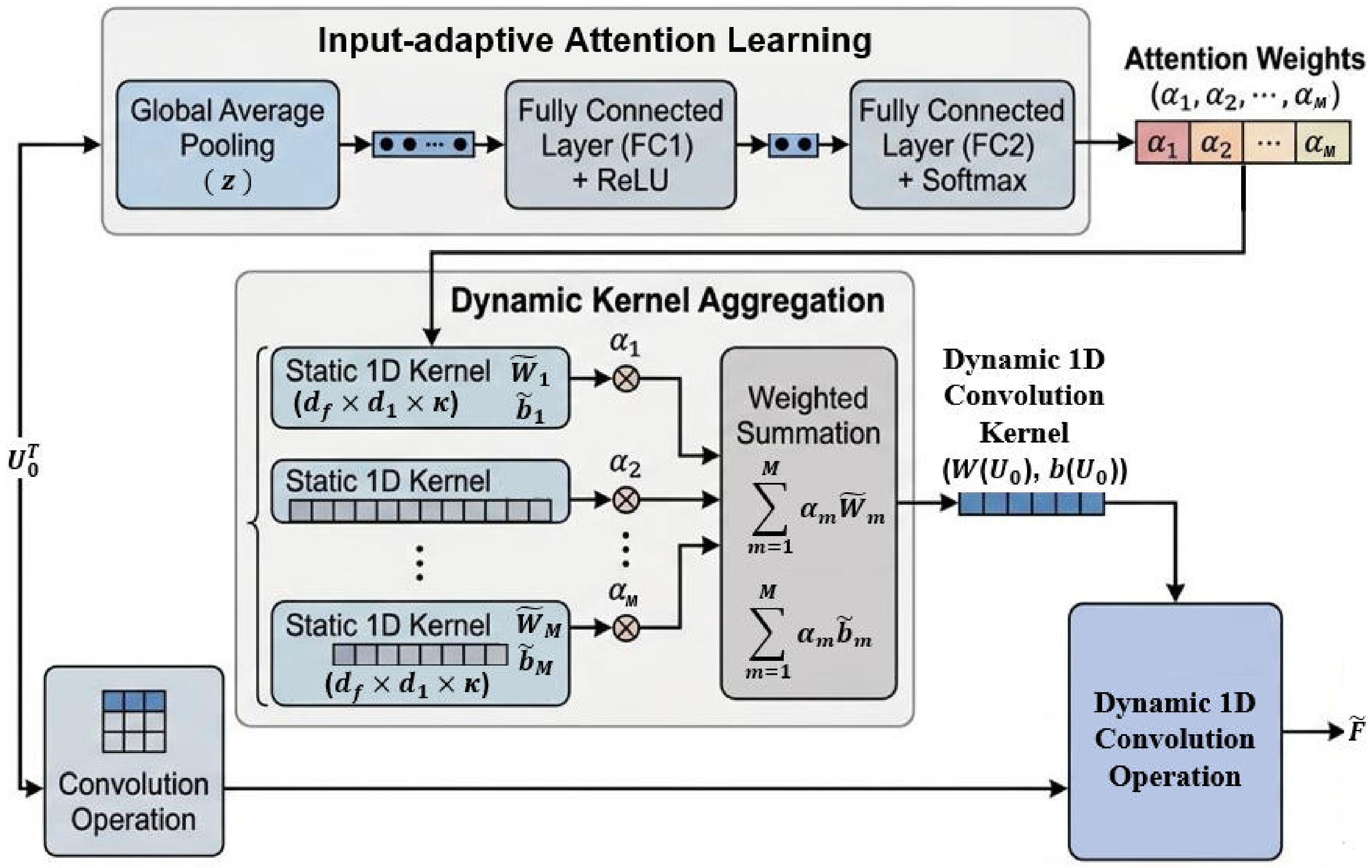
To fully exploit the information within $U_0$, we propose a novel architecture that integrates input-adaptive dynamic one-dimensional convolution with Transformer for energy demand forecasting. Instead of directly using the traditional convolution, we adopt the idea of dynamic convolution [33] and adapt it to one-dimensional time-series data. The traditional static convolution applies the same set of kernels to every input sample, which may limit its ability to adapt to dynamically changing data. To overcome this shortcoming, we dynamically change the parameters of M one-dimensional convolution kernels using input-dependent attention weights. In this way, our dynamic convolution no longer applies the same shared convolution kernel parameters to all inputs as in traditional convolution. Specifically, we use multiple convolution kernels of the same size. The parameters of these kernels are adaptively learned from the input data. As shown in Figure 2, the learned kernels are then convolved with the input. As a result, we can enhance the representation capability of our method by using adaptively dynamic convolution, while still leveraging the powerful sequence modeling ability of the Transformer.

Specifically, the input $U_0$ is first transposed to enable convolution along the channel dimension, thus fully capturing the complex relationships among different feature variables. Subsequently, global average pooling is used to compress the transposed $U_0$ over the channel dimension. Two fully connected layers are further used to produce a score vector $s_m\in {\mathbb{R}}^1$. To obtain normalized attention weights $\alpha$, we apply a softmax function. The convolved result is further passed through batch normalization and a ReLU activation to yield the final output. The output F of dynamic convolution can be formulated as follows:

$$\begin{array}{cc}\hfill & z={\displaystyle \frac{1}{C}}{\displaystyle \sum _{i=1}^C}{U}_0^T[:,i]\hfill \\ \hfill & s_m=W_{2}ReLU(W_{1}z+b_1)+b_2\hfill \\ \hfill & {\alpha }_m={\displaystyle \frac{exp\left(s_m\right)}{{\sum }_{i=1}^{M}exp\left(s_i\right)}}\hfill \\ \hfill & \tilde{W}\left(U_0\right)={\displaystyle \sum _{m=1}^M}{\alpha }_m{\tilde{W}}_m,\tilde{b}\left(U_0\right)={\displaystyle \sum _{m=1}^M}{\alpha }_m{\tilde{b}}_m\hfill \\ \hfill & \tilde{F}=\mathrm{Conv}1\mathrm{D}\left(U_0,\tilde{W}\left(U_0\right),\tilde{b}\left(U_0\right),\mathrm{stride}=ϵ,\mathrm{padding}=p\right)\hfill \\ \hfill & F=ReLU\left(BatchNorm\left(\tilde{F}\right)\right)\hfill \end{array}$$

(6)

where $z\in {\mathbb{R}}^{d_1}$, $W_1\in {\mathbb{R}}^{d_1\times d_1}$, $b_1\in {\mathbb{R}}^{d_1}$, $W_2\in {\mathbb{R}}^{M\times d_1}$, and $b_2\in {\mathbb{R}}^M$. ${\tilde{W}}_m\in {\mathbb{R}}^{d_f\times d_1\times \kappa }$ and ${\tilde{b}}_m\in {\mathbb{R}}^{d_f}$ are the weight and bias of the m-th kernel, respectively. $F\in {\mathbb{R}}^{d_f\times d_c}$. $d_c=\lfloor (C+2p-\kappa )/ϵ\rfloor +1$. $\mathrm{Conv}1\mathrm{D}(·), ReLU(·)$, and $BatchNorm(·)$ denote the one-dimensional convolution operation, ReLU activation function, and batch layer normalization function, respectively.

Then, we add a learnable positional encoding $E_{\mathrm{pos}}$ to F and input it into a Transformer encoder with $L_1$ layers. Since the dynamic convolution primarily targets inter-variable feature extraction, the learned channel information is predominantly encoded along the $d_c$ dimension. Hence, to further capture additional characteristics from F, we first transpose the dimensions of F and process it with a Transformer encoder. For each layer of the Transformer encoder, it contains a multi-head self-attention (MHSA) sub-layer and a position-wise feed-forward network (FFN), both with residual connections and layer normalization. As for each head h in MHSA, the input G is projected to queries, keys, and values. The outputs from all the heads are concatenated and linearly projected as follows:

$$\begin{array}{cc}\hfill & G=F^{\top }+E_{\mathrm{pos}}\hfill \\ \hfill & Q_h=G{W}_h^Q,K_h=G{W}_h^K,V_h=G{W}_h^V\hfill \\ \hfill & {\mathrm{Attn}}_h\left(G\right)=\mathrm{softmax}\left({\displaystyle \frac{Q_h{K}_h^{\top }}{\sqrt{d_k}}}\right)V_h\hfill \\ \hfill & \mathrm{MHSA}\left(G\right)=\mathrm{Concat}({\mathrm{Attn}}_1\left(G\right),\dots ,{\mathrm{Attn}}_{d_a}\left(G\right))W^O\hfill \end{array}$$

(7)

where $G\in {\mathbb{R}}^{d_c\times d_f},W_h^Q,W_h^K\in {\mathbb{R}}^{d_f\times d_k}$, $W_h^V\in {\mathbb{R}}^{d_f\times d_v}$, and $d_k=d_v=d_f/d_a$. $d_a$ denotes the number of heads. $W^O\in {\mathbb{R}}^{d_a{d}_v\times d_f}$.

After the MHSA computation, we further perform residual connection, layer normalization, and FFN operations to obtain the output of the i-th Transformer encoder layer.

$$\begin{array}{cc}\hfill & \tilde{G}=\mathrm{LayerNorm}(G+\mathrm{MHSA}\left(G\right))\hfill \\ \hfill & G^{\left(i\right)}=\mathrm{LayerNorm}(\tilde{G}+\mathrm{ReLU}(\tilde{G}{W}_3+b_3)W_4+b_4)\hfill \end{array}$$

(8)

where $W_3\in {\mathbb{R}}^{d_f\times d_g}$, $b_3\in {\mathbb{R}}^{1\times d_g}$, $W_4\in {\mathbb{R}}^{d_g\times d_f}$, and $b_4\in {\mathbb{R}}^{1\times d_f}$.

Finally, we stack $L_1$ such layers, and can then obtain the final encoded representation $G^{\left(L_1\right)}\in {\mathbb{R}}^{d_c\times d_f}$, which is further processed by a linear transformation to predict the final energy demand.

$$\tilde{y}=G^{\left(L_1\right)}{W}_{\mathrm{pred}}+b_{\mathrm{pred}}$$

(9)

where $\tilde{y}\in {\mathbb{R}}^{d_o}$. $d_o$ is the output dimension. $W_{\mathrm{pred}},b_{\mathrm{pred}}\in {\mathbb{R}}^{d_f\times 1}$.

3.4. Bayesian Optimization for Hyperparameter Tuning

To improve the efficiency of hyperparameter optimization, we treat the hyperparameters a, including the learning rate, period length P, kernel size, $d_1$, $L_1$, and so on, as discrete parameters. Taking the learning rate as an example, its value ranges from $1\times {10}^{-7}$ to $9\times {10}^{-3}$ with a step size of $1\times {10}^{-7}$. In this way, the entire hyperparameter optimization problem is transformed into a combinatorial optimization problem. As for the hyperparameter optimization method, we introduce an efficient TPE [46]. In TPE, we do not adopt the traditional Aitchison–Aitken kernel but use an improved kernel function. The technical details are as follows.

Let $\mathcal{D}:={\left\{(a_n,f\left(a_n\right))\right\}}_{n=1}^{N_0}$ be the set of $N_0$ observed hyperparameter configurations and their corresponding objective values. Here, the optimization objective is to minimize the prediction error on the validation set. Instead of directly modeling the objective function, we construct two nonparametric density estimators using a split of the observed data based on a quantile threshold. Define $f^{\prime }$ as the $\gamma$-quantile of the observed objective values ${\left\{f\left(a_n\right)\right\}}_{n=1}^{N_0}$. Using this threshold, we partition $\mathcal{D}$ into two disjoint subsets, namely,

$${\mathcal{D}}_{\mathrm{good}}:=\{(a,f)\in \mathcal{D}\mid f<f^{\prime }\},{\mathcal{D}}_{\mathrm{bad}}:=\mathcal{D}\setminus {\mathcal{D}}_{\mathrm{good}}.$$

(10)

where ${\mathcal{D}}_{\mathrm{good}}$ contains the configurations yielding the best (lowest) objective values. ${\mathcal{D}}_{\mathrm{bad}}$ contains the remaining ones. $\gamma \in [0,1]$ is a heuristic parameter.

Next, we build two Parzen density estimators: one for the good configurations and one for the bad ones. For any candidate hyperparameter a, the densities are expressed as follows:

$$\begin{array}{cc}\hfill & p(a\mid {\mathcal{D}}_{\mathrm{good}})={\displaystyle \frac{1}{|{\mathcal{D}}_{\mathrm{good}}|}}\sum _{(a^{\prime },·)\in {\mathcal{D}}_{\mathrm{good}}}{\displaystyle \frac{m(a,a^{\prime })}{Z\left(a^{\prime }\right)}}\hfill \\ \hfill & p(a\mid {\mathcal{D}}_{\mathrm{bad}})={\displaystyle \frac{1}{|{\mathcal{D}}_{\mathrm{bad}}|}}\sum _{(a^{\prime },·)\in {\mathcal{D}}_{\mathrm{bad}}}{\displaystyle \frac{m(a,a^{\prime })}{Z\left(a^{\prime }\right)}}\hfill \\ \hfill & m(a,a^{\prime })={\displaystyle \prod _{d=1}^D}{m}_d(a_d,a_d^{\prime })\hfill \end{array}$$

(11)

where $m(·,·)$ is a kernel function, and $Z\left(a^{\prime }\right):={\int }_{\theta \in \mathcal{X}}m(\theta ,a^{\prime })d\theta$ is a normalization factor ensuring that each term integrates to one over the domain $\mathcal{X}$. The kernel $m(·,·)$ is assumed to factorize across the D dimensions of the hyperparameter vector $a=(a_1,a_2,\dots ,a_D)$.

Considering that the standard Aitchison–Aitken kernel in TPE treats all category values symmetrically, it may disregard any prior knowledge about their similarities. This limitation becomes severe when the optimization problem involves categorical hyperparameters with inherent distances or orders [46]. Hence, we mitigate this issue by incorporating a user-defined distance metric between categorical combinations, thereby enabling more efficient Bayesian optimization for our method. We define a metric $M_d:{\mathcal{X}}_d\times {\mathcal{X}}_d\to {\mathbb{R}}_{\ge 0}$. The $m_d(a_d,a_d^{\prime })$ can then be formulated as follows:

$$\begin{array}{cc}\hfill & m_d(a_d,a_d^{\prime })=exp\left(-{\displaystyle \frac{1}{2}}{\left({\displaystyle \frac{M_d(a_d,a_d^{\prime })}{\beta }}\right)}^2\right)\hfill \\ \hfill & \beta ={\displaystyle \frac{M_d^{\max }}{\sqrt{2log\frac{C_d-1}{d_p}}}}\hfill \end{array}$$

(12)

where $M_d^{\max }:={max}_{[a_d^{\left(1\right)},a_d^{\left(2\right)}]\in {\mathcal{X}}_d\times {\mathcal{X}}_d}{M}_d(a_d^{\left(1\right)},a_d^{\left(2\right)})$. $C_d$ is the number of categories for the categorical parameter of $a_d$, and $d_p$ is a constant.

According to these two density estimates, the next hyperparameter configuration $a_{N_0+1}$ is chosen by maximizing the ratio of the good density to the bad density. In practice, we first use a Monte Carlo sampling strategy to sample a set of candidate points $\mathcal{S}\subseteq \mathcal{X}$ from $p(a\mid {\mathcal{D}}_{\mathrm{good}})$ and then select the point that maximizes the ratio. Intuitively, this criterion naturally directs the search toward regions where $p(a\mid {\mathcal{D}}_{\mathrm{good}})$ is large and $p(a\mid {\mathcal{D}}_{\mathrm{bad}})$ is small. The $a_{N_0+1}$ can be selected based on the following density ratio:

$$a_{N_0+1}\in arg\underset{a\in \mathcal{S}}{max}{\displaystyle \frac{p(a\mid {\mathcal{D}}_{\mathrm{good}})}{p(a\mid {\mathcal{D}}_{\mathrm{bad}})}}.$$

(13)

In summary, the whole procedure consists of evaluating the objective at the selected point, updating the dataset, and recomputing the densities. This process is repeated iteratively until a budget of evaluations is exhausted or convergence is achieved.

4. Experiments and Discussion

To investigate our method’s effectiveness, we selected two energy demand forecasting tasks with multivariate factors. The first task focuses on forecasting total energy use for multiple energy sources. It relies on historical energy-load records, weather conditions, and other demand-related multivariate variables. Similarly, the second task is to forecast the national electricity load in Panama.

For convincing comparison, we selected several state-of-the-art methods from the past three years as baselines for comparison, including different architectures, such as recurrent neural network-based SKOLR [47], graph neural network-based FCSTGNN [48], Transformer-based iTransformer [49], and EMAformer [45]. Moreover, we also used several hybrid methods, including MSGNet [50], TimeKan [51], FreDN [52], and CaberNet [38]. All the comparative experiments were conducted under the same conditions. Here, we evaluate the prediction performance using three standard regression metrics: the coefficient of determination (${\mathrm{R}}^2$), mean absolute percentage error (MAPE), and coefficient of variation of the root mean square error (CV-RMSE):

$$\begin{array}{cc}\hfill & {\mathrm{R}}^2=1-{\displaystyle \frac{{\sum }_{i=1}^N{({\tilde{y}}_i-y_i)}^2}{{\sum }_{i=1}^N{(\overline{y}-y_i)}^2}}\hfill \\ \hfill & \mathrm{MAPE}={\displaystyle \frac{1}{N}}{\displaystyle \sum _{i=1}^N}|{\displaystyle \frac{{\tilde{y}}_i-y_i}{y_i}}|\times 100\%\hfill \\ \hfill & \mathrm{CV}\text{-}\mathrm{RMSE}={\displaystyle \frac{\sqrt{\frac{1}{N}{\sum }_{i=1}^N{({\tilde{y}}_i-y_i)}^2}}{\overline{y}}}\times 100\%\hfill \end{array}$$

(14)

where $y_i$, ${\tilde{y}}_i$, and $\overline{y}$ denote the actual value, predicted value, and mean of actual values, respectively. N denotes the total number of samples.

In all the experiments, the optimizer was Adam, and the normalization method employed was Z-score standardization. Missing values were removed directly. The batch size, the random seed, the number of initial samples, the maximum number of iterations, $ϵ$, and L were set to 128, 3407, 10, 100, 1, and 3, respectively. We adopted the same padding. The search range for the learning rate was from $1\times {10}^{-7}$ to $9\times {10}^{-3}$, with a step size of $1\times {10}^{-7}$. $d_1$, $d_f$, $\kappa$, P, and $L_1$ were selected from the sets {64, 128, 256, 512, 640, 768}, {64, 128, 256, 512, 640, 768, 1024}, {3, 5, 7}, {7, 24, 30, 60, 168, 360}, and {2, 3, 4, 5}, respectively. In the hyperparameter optimization, (1−${\mathrm{R}}^2$) was adopted as the optimization objective. The final hyperparameter configuration after optimization can be summarized as follows. For the two cases, the learning rates were $5\times {10}^{-6}$ and $3\times {10}^{-6}$, respectively. The values of $d_1$ and $d_f$ are (128, 128) and (512, 512), respectively. The values of $\kappa$ and P are (3, 360) and (5, 168), respectively. The value of $L_1$ is 3. Experiments were conducted on a computer equipped with an Intel Core i7-13700 CPU, 128 GB of memory, and an NVIDIA GeForce RTX 4090 GPU. The source code will be available at https://github.com/entask26/dconvformer (accessed on 2 September 2026).

4.1. An Energy Demand Forecasting Case in Spain

Here, we used an energy demand forecasting case in Valencia, Spain. In this case, there are multiple influencing factors, including generation types such as biomass, fossil gas, fossil hard coal, fossil oil, hydro run-of-river and poundage, hydro water reservoir, nuclear, solar, waste, and onshore wind, as well as weather-related variables like temperature, air pressure, humidity, wind speed, rainfall, weather conditions, and energy prices. The original dataset is available at https://github.com/ritikdhame/Electricity_Demand_and_Price_forecasting (accessed on 2 September 2026). To predict the total energy demand, we selected several variables, including temperature (°C), humidity (%), 3-h rainfall (mm), pressure (hPa), wind speed (km/h), wind direction (°), weather description, energy price, and the previous energy demand (MW). This dataset was recorded hourly from 1 January 2015 to 31 December 2018, and contained 35,050 samples. It is split into three subsets in chronological order, with 70% for training, 10% for validation, and 20% for testing.

Table 1. Comparative results on the case in Spain. The best results are highlighted in bold.

Method	${\mathbf{R}}^2$	MAPE (%)	CV-RMSE (%)
FCSTGNN [48]	0.9459	2.6233	3.6384
MSGNet [50]	0.8871	4.0073	5.2608
iTransformer [49]	0.823	5.0281	6.587
SKOLR [47]	0.8994	3.7318	4.9669
TimeKan [51]	0.645	7.1732	9.3282
FreDN [52]	0.5401	8.1036	10.6182
EMAformer [45]	0.8798	4.0558	5.429
CaberNet [38]	0.8006	5.4886	6.9920
Ours	0.9465	2.4626	3.6229

presents the quantitative comparison between our method and eight advanced forecasting models. It clearly shows that our method outperforms all the comparative methods with respect to all the evaluation metrics. Specifically, for two advanced Transformer variants, iTransformer and EMAformer, their CV-RMSE values stand at 6.587% and 5.429%, respectively. However, our method maintains a much lower error of 3.6229%. As for other advanced methods, such as MSGNet, FreDN and CaberNet, most of them exhibit relatively high error rates, with MAPE scores above 4% and CV-RMSE values exceeding 5%.

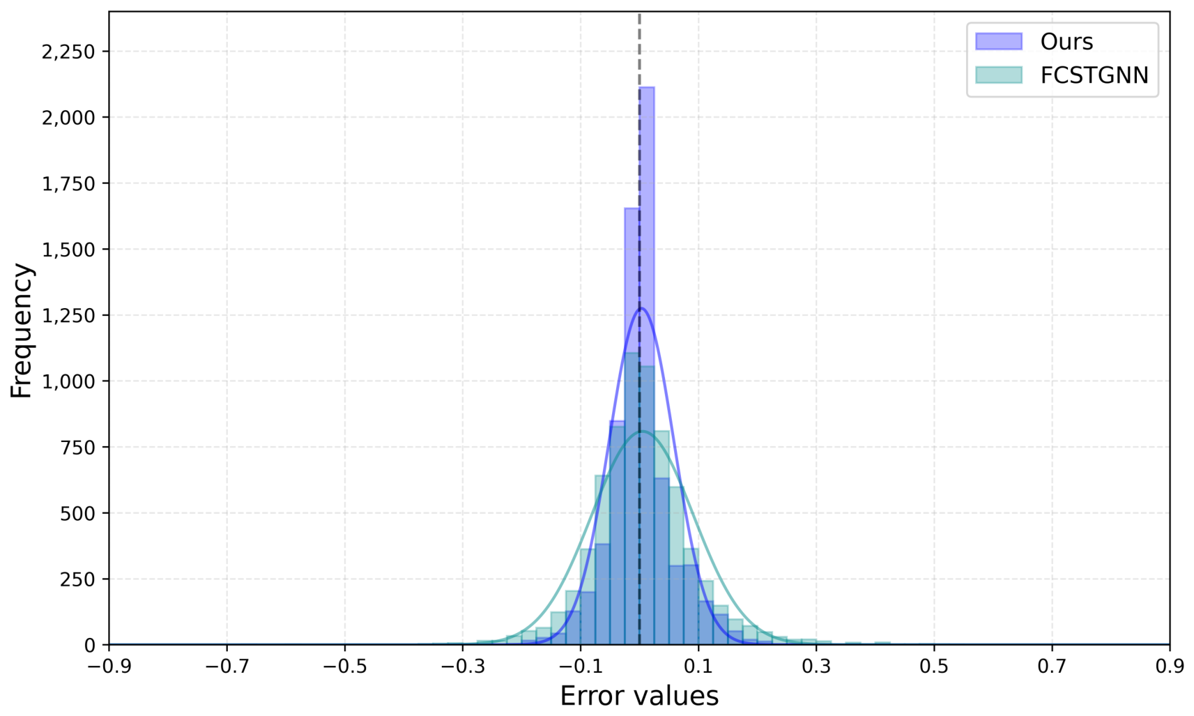
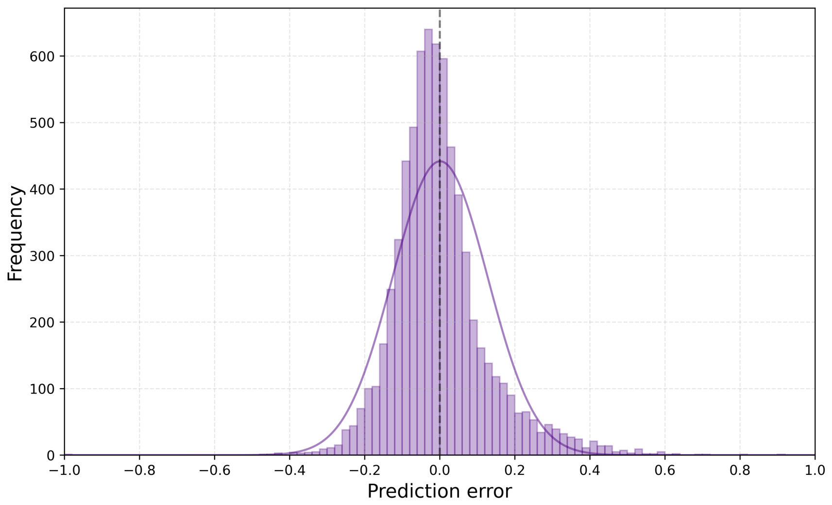
Since the superiority of our method over the second-best method is not very significant in numerical terms, we further conducted a visual comparative analysis. Figure 3 illustrates a histogram comparison of the prediction errors between our method and the second-best baseline model. As observed, the distribution for our method exhibits an extremely sharp, narrow, and concentrated peak centered exactly at zero. This indicates that the vast majority of our predictions are highly precise, with minimal variance. In contrast, the FCSTGNN shows a notably broader and more dispersed bell-shaped distribution, along with significantly longer tails on both the positive and negative sides. The results show that the prediction error distribution of our method is better than that of FCSTGNN.

The superiority of our method can be illustrated as follows. Our method benefits from the synergistic combination of channel–phase embeddings and adaptive dynamic convolution. The embeddings provide a richer initial representation that encodes both stable inter-channel relationships and periodic phase information. Although EMAformer is capable of providing diverse feature embedding representations, it lacks the adaptive learning capability inherent in dynamic convolution. Our dynamic convolution can achieve adaptively convolutional computation based on the input itself. It extracts more relevant features before the sequence is passed to the Transformer encoder. As a result, our method can efficiently predict the energy demand.

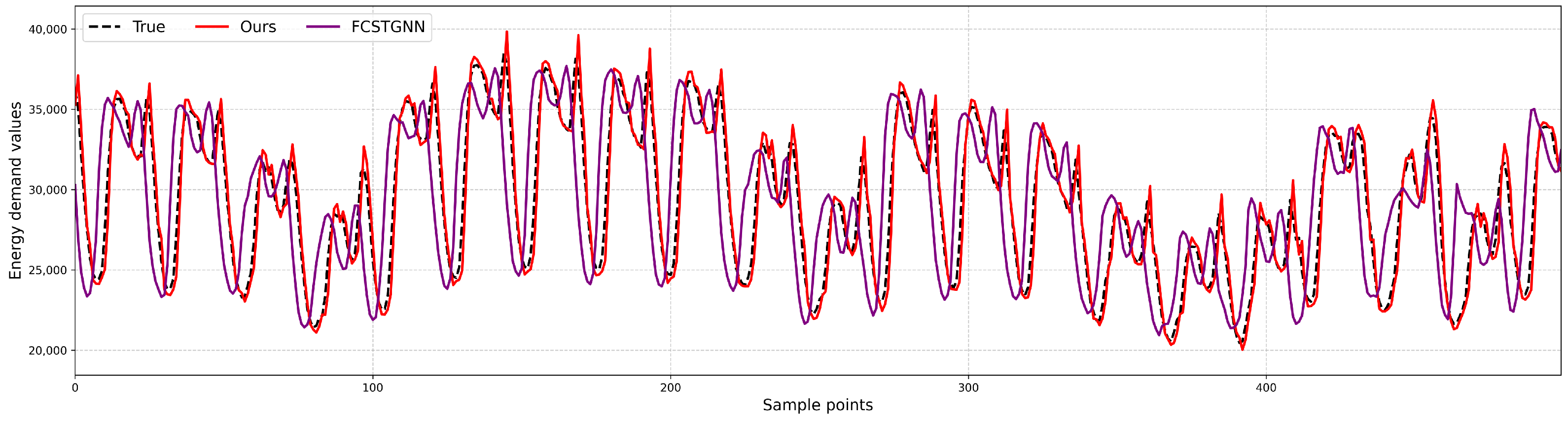
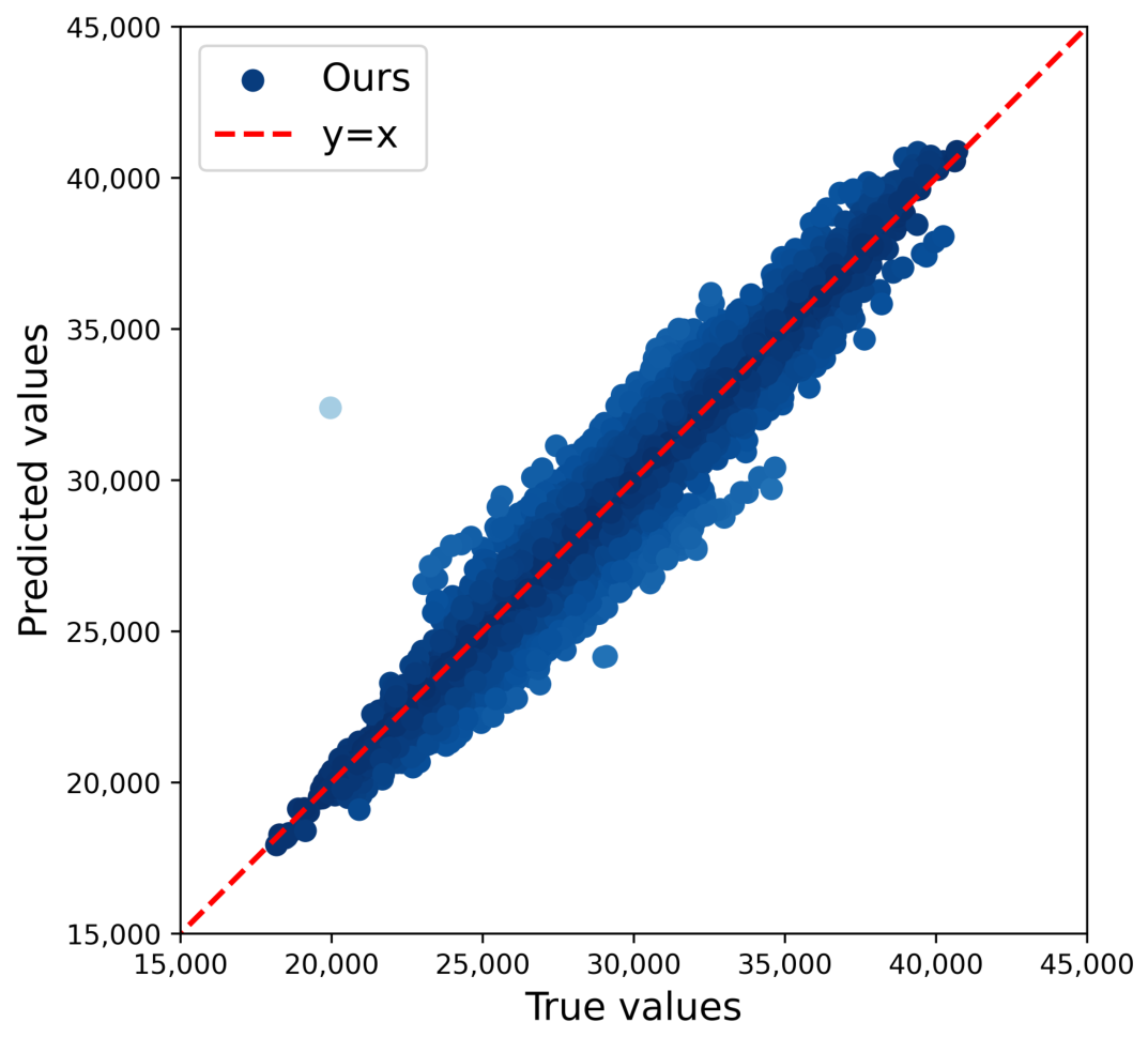
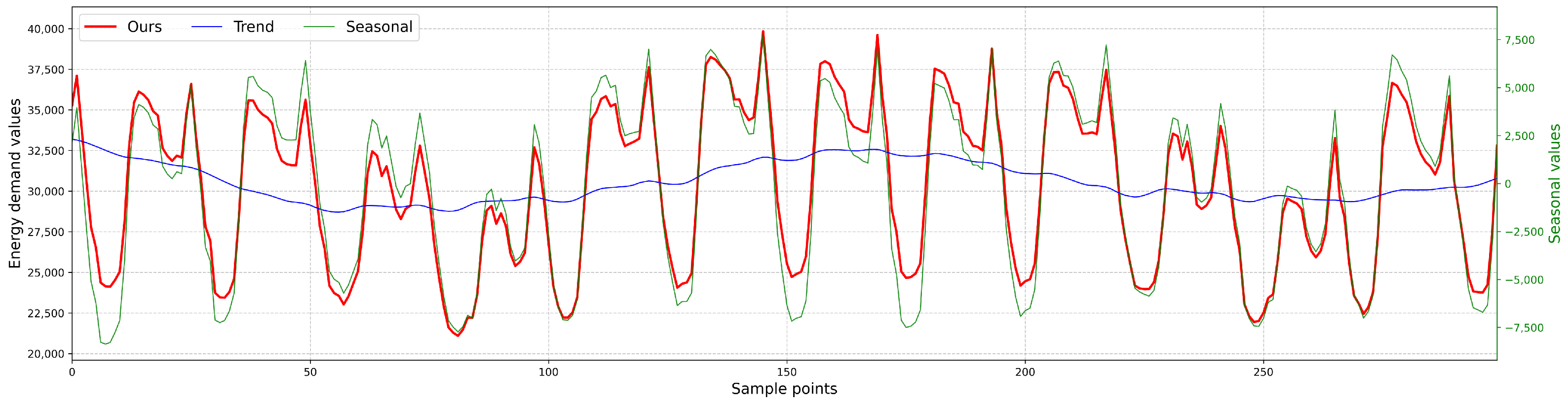
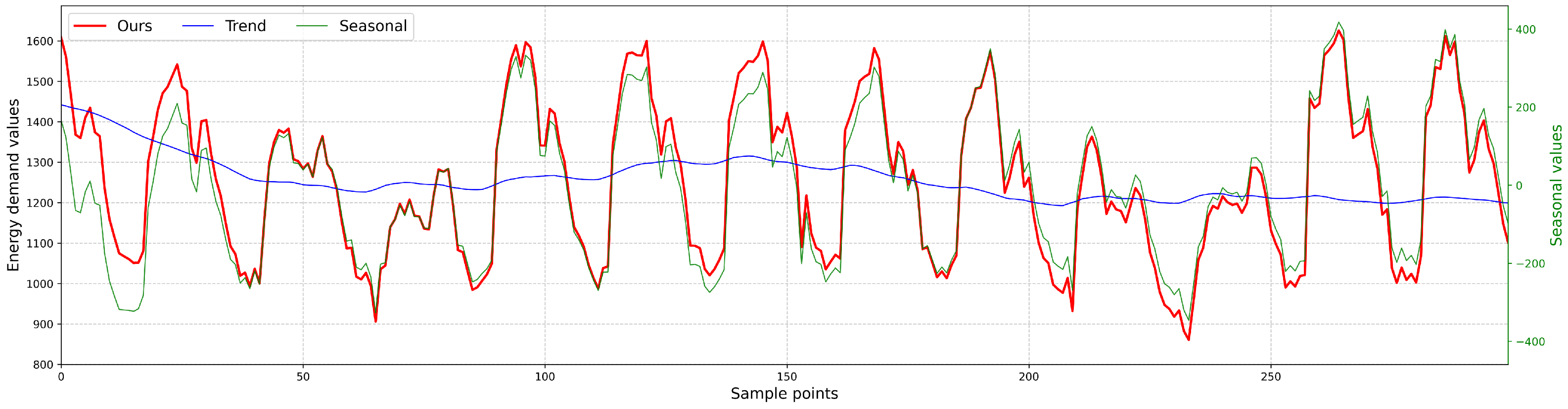
As shown in Figure 4, we present a segment of the prediction curves to clearly compare our method with the second-best one. It can be seen that the predicted energy demand values of our method closely follow the true values across all the time steps. There is no obvious lag or systematic bias in the forecasts. However, the FCSTGNN method, with the second-best performance, shows clear lags in its predictions. Its performance disadvantage becomes more evident when energy demand changes suddenly or drastically. Figure 5 presents a scatter plot of our predictions against the true values. Most points lie near the diagonal line, indicating a strong linear correlation. Only a few points deviate slightly from the line. In addition to the prediction results, we also present their trend and seasonal components. Figure 6 shows that energy demand exhibits clear seasonal variation and cyclical upward and downward trends. This visual evidence explicitly confirms that our method can accurately capture both the magnitude and the fluctuations of the energy demand.

4.2. An Energy Demand Forecasting Case in Panama

In this case, a curated hourly national energy consumption dataset in Panama was collected to validate the effectiveness of our proposed method. The complete dataset contains 48,048 observations spanning from 3 January 2015 to 26 June 2020. Here, the specific energy refers to electrical load. It comes from daily post-dispatch reports published by the grid operator. The calendar information regarding school periods is obtained from the Ministry of Education of Panama. Public holiday schedules are acquired from the “When on Earth” website. There are a total of 22 distinct types of statutory and cultural holidays. The weather variables are retrieved from the Earthdata platform. The target variable represents the national electricity load measured in megawatt hours. The exogenous predictors are systematically categorized into meteorological features and temporal indicators. The meteorological features include temperature at two meters and relative humidity along with liquid precipitation and wind speed. These weather parameters are collected from geographically dispersed monitoring stations in Tocumen, Santiago, and David. The temporal indicators comprise dichotomous flags for holidays and school terms. The original dataset is available at https://data.mendeley.com/datasets/byx7sztj59/1 (accessed on 2 September 2026). A full variable dictionary with units and data types is provided in

Table 2. Variable description.

Variable Name	Description	Unit
T2M_toc	Temperature at 2 m in Tocumen, Panama City	°C
QV2M_toc	Relative humidity at 2 m in Tocumen, Panama City	%
TQL_toc	Liquid precipitation in Tocumen, Panama City	L/m2
W2M_toc	Wind speed at 2 m in Tocumen, Panama City	m/s
T2M_san	Temperature at 2 m in Santiago city	°C
QV2M_san	Relative humidity at 2 m in Santiago city	%
TQL_san	Liquid precipitation in Santiago city	L/m2
W2M_san	Wind speed at 2 m in Santiago city	m/s
T2M_dav	Temperature at 2 m in David city	°C
QV2M_dav	Relative humidity at 2 m in David city	%
TQL_dav	Liquid precipitation in David city	L/m2
W2M_dav	Wind speed at 2 m in David city	m/s
Holiday_ID	Unique identification number	integer
Holiday	Holiday binary indicator (holiday: 1/regular: 0)	0, 1
School	School period binary indicator (school: 1/vacation: 0)	0, 1
Nat_demand	National electricity load (target variable)	MWh

. Here, we also use 70% of the dataset for training, 10% for validation, and 20% for testing.

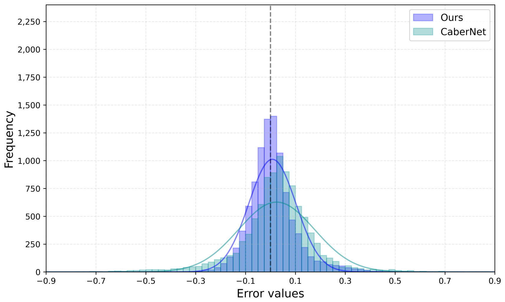
As shown in

Table 3. Comparative results on the case in Panama.

Method	${\mathbf{R}}^2$	MAPE (%)	CV-RMSE (%)
FCSTGNN [48]	0.8882	3.5819	5.1304
MSGNet [50]	0.911	3.5344	4.5771
iTransformer [49]	0.8261	4.8117	6.3998
SKOLR [47]	0.9297	3.1365	4.0698
TimeKan [51]	0.7001	5.8499	8.4026
FreDN [52]	0.6679	6.304	8.8428
EMAformer [45]	0.9391	2.9349	3.7882
CaberNet [38]	0.9418	2.6651	3.7013
Ours	0.9611	2.1542	3.0277

, our method also outperforms all the comparative methods across all evaluation metrics. Compared with graph-based methods like FCSTGNN and MSGNet, our method reduces the CV-RMSE forecasting by approximately 41.0% and 33.9%, respectively. Compared with the Transformer variants, including iTransformer, EMAformer, and FreDN, our method reduces the CV-RMSE by at least approximately 20.1% and by up to approximately 65.76%. As for other advanced methods, including SKOLR and TimeKan, our method has an advantage across all the evaluation metrics. Even when compared to the method ranked second in overall performance, our method still maintains a certain advantage. As shown in Figure 7, our error distribution exhibits a much higher peak and a tighter concentration around zero. However, the error curve for CaberNet shows a wider spread and a lower frequency at the center. This direct comparison also confirms the effectiveness of our method.

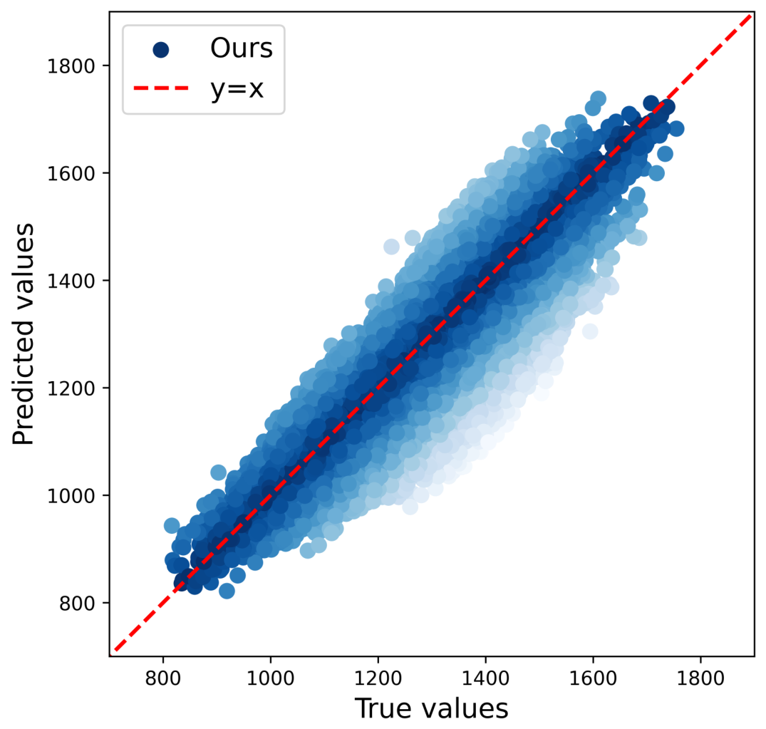
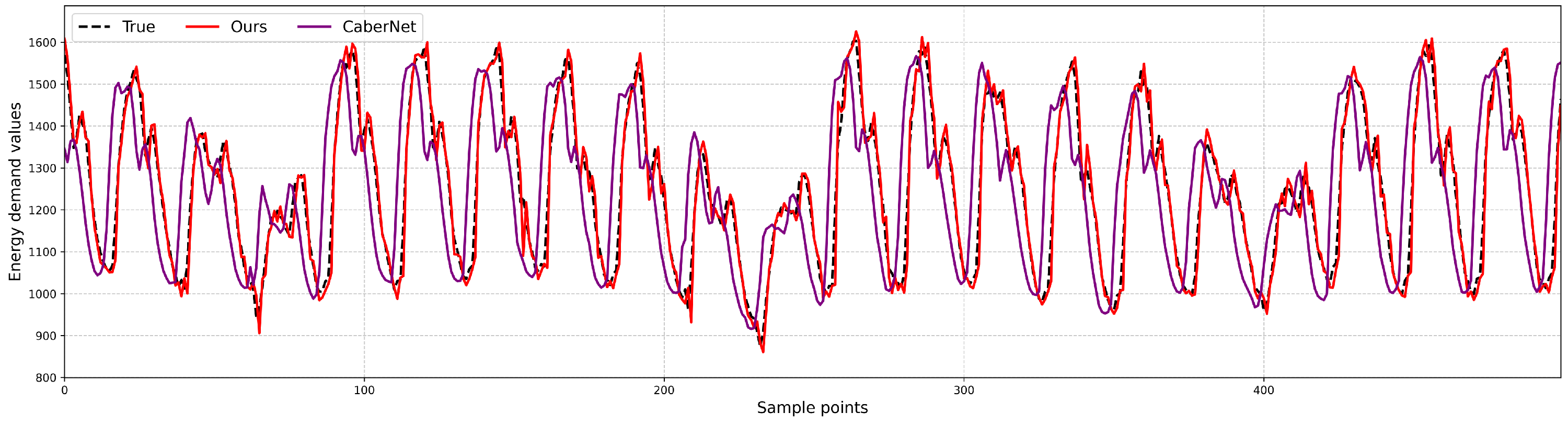
Figure 8 shows that our predicted demand aligns well with the actual data. No significant delays or consistent errors appear in the results. However, the second-best method CaberNet still exhibits clear lag in its predictions, and when energy demand changes suddenly or drastically, it still underperforms our method. Figure 9 displays the scatter plot that compares our predicted results with the corresponding real ones. Most points lie near the diagonal line. This phenomenon reflects an exceptionally strong linear matching relationship between predictions and real observations. As shown in Figure 10, the seasonality and trend predicted by our method are similar to those in the previous case, both showing relatively clear seasonal variation and a non-monotonic trend. All these visual results strongly confirm that our method can capture both the scale and dynamics of energy demand.

In summary, the quantitative and qualitative results highlight the effectiveness of our method. The combination of channel–phase embeddings and adaptive dynamic convolution leads to accurate forecasts. Hence, our method is a practical solution for energy demand forecasting.

4.3. Ablation Experiments

To verify the necessity and effectiveness of each module in our method, we further conduct ablation studies. We use our full method as the baseline model and conduct ablation experiments by removing each of the proposed modules. Specifically, ‘ThrEmd’ denotes the inclusion of all three embeddings (channel, phase, and joint channel–phase embeddings), while ‘Dconv’ denotes the dynamic convolution module. ‘w/o ThrEmd’ and ‘w/o Dconv’ indicate that ‘ThrEmd’ and ‘Dconv’ are removed from our method, respectively. ‘w/o ThrEmd, Dconv’ indicates that both components are removed. This variant is essentially the Transformer. ‘w/channel’, ‘w/phase’, and ‘w/channel–phase’ denote the variants where ‘ThrEmd’ is replaced by channel-only, phase-only, and joint channel–phase embeddings, respectively. ‘w/randSearch’ denotes the variant where the Bayesian optimizer is replaced with random search.

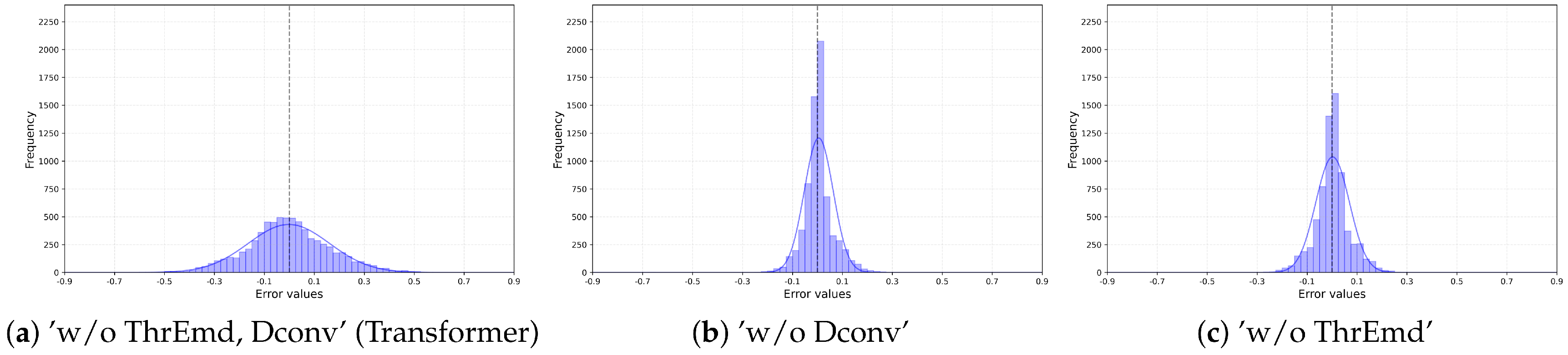
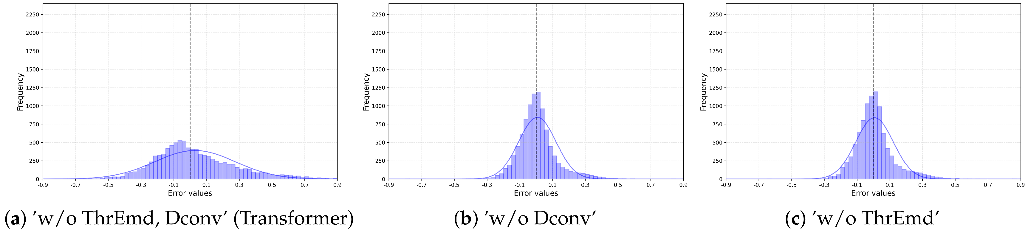
According to

Table 4. Ablation results on the case in Spain.

Module	${\mathbf{R}}^2$	MAPE (%)	CV-RMSE (%)
w/o ThrEmd, Dconv	0.7790	5.8573	7.3617
w/o Dconv	0.9436	2.5345	3.7179
w/o ThrEmd	0.9413	2.7140	3.7948
w/phase	0.9432	2.5426	3.7330
w/channel	0.9381	2.7712	3.8944
w/channel–phase	0.9431	2.5488	3.7353
w/randSearch	0.9350	2.8900	3.9912
Ours	0.9465	2.4626	3.6229

and

Table 5. Ablation results on the case in Panama.

Module	${\mathbf{R}}^2$	MAPE (%)	CV-RMSE (%)
w/o ThrEmd, Dconv	0.8752	4.1284	5.4218
w/o Dconv	0.9542	2.3328	3.2862
w/o ThrEmd	0.9489	2.4655	3.4695
w/phase	0.9594	2.2287	3.0937
w/channel	0.9547	2.3200	3.2651
w/channel–phase	0.9560	2.2912	3.2186
w/randSearch	0.9580	2.2431	3.1441
Ours	0.9611	2.1542	3.0277

, we conducted a comparative analysis from three aspects. (1) By comparing ‘w/o ThrEmd’, ‘w/phase’, ‘w/channel’ and ‘w/channel-phase’ with our full method, we found that all proposed embedding strategies were effective. This indicates that explicit channel position embedding indeed helps the model capture relationships within and between channels. Meanwhile, explicit phase embedding can help the model extract latent periodic features from the data and thus improve learning efficiency. Moreover, the joint use of these embeddings can produce synergistic effects and further improve the algorithmic performance. In addition, ‘w/phase’ achieved higher prediction accuracy than ‘w/channel’. The possible reason is as follows. As shown in Figure 4 and Figure 8, both datasets exhibit latent periodic characteristics. Phase embedding explicitly characterizes this property and is clearly more informative than channel embedding, which provides only positional information. Since the model can exploit more feature information from the data, ‘w/phase’ may contribute more to performance improvement. (2) By comparing ‘w/o Dconv’ with our method, and ‘w/o ThrEmd, Dconv’ with ‘w/o ThrEmd’, we found that dynamic convolution indeed improved algorithm performance. Compared with the standalone Transformer, the introduced dynamic convolution improved ${\mathrm{R}}^2$ by at least 8.4%. This indicates that input-dependent adaptive convolution indeed captures correlations among different variables and thus improves performance. As shown in Figure 11 and Figure 12, dynamic convolution and ‘ThrEmd’ both significantly improve Transformer’s prediction performance, and their prediction error distributions are concentrated near zero. (3) Compared with ‘w/randSearch’, our Bayesian optimization method achieves better optimization performance under the same conditions. This indicates that the kernel density estimation-based Bayesian optimization method can indeed improve the optimization efficiency and achieve better optimization results than random search.

In summary, each module effectively improves the forecasting accuracy, and both are indispensable for achieving the best performance.

4.4. Discussion

Although the experimental results in the previous section confirm the effectiveness of our method, they are based on limited cases and comparison experiments. To further validate the effectiveness of our method, we analyzed it from both the theoretical and practical perspectives.

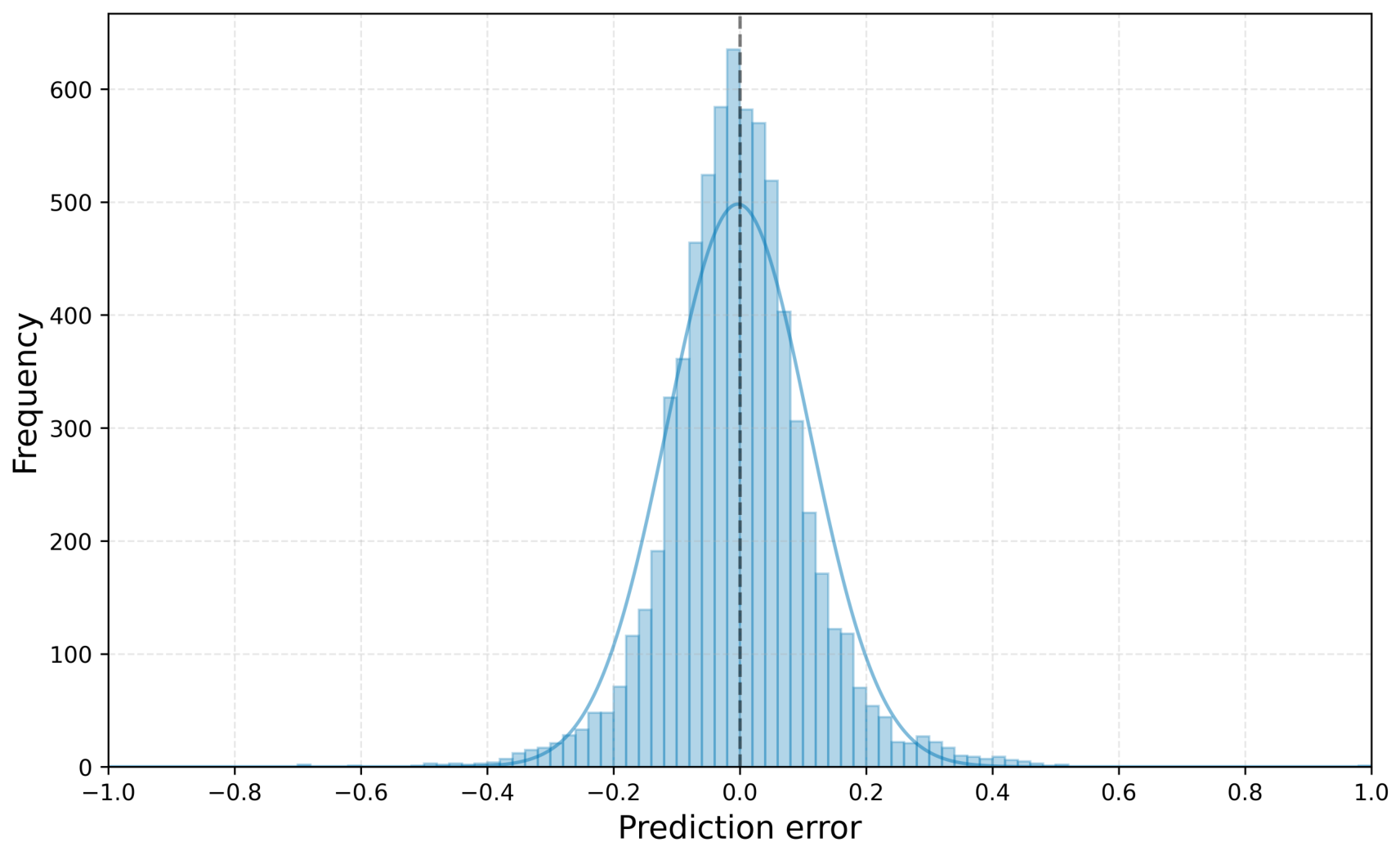
(1) Theoretically, the advantages of our method in the above comparative experiments can be mainly attributed to two aspects. (1) From the perspective of feature embedding, the triple embedding strategy can provide rich input representation, thus helping our method extract both temporal periodicity and channel characteristics. Specifically, the channel embedding provides stable inter-channel relationships, while the phase embedding captures periodic patterns such as daily or weekly cycles. The joint embedding models fine-grained interactions between each channel and its current phase. As shown in the ablation study, adding only the triple embedding module reduces the CV-RMSE scores by at least approximately 39.4% and by up to approximately 49.5%. It also reduces MAPE scores by at least approximately 43.5% and by up to approximately 56.7%. (2) From the perspective of dynamic convolution, it replaces a fixed static kernel with input-dependent one. This allows the method to adaptively extract features according to the input. When both the triple embeddings and the dynamic convolution are used together with Bayesian optimization, the full method achieves the best results across all evaluation metrics. The combination of better input representations, adaptive feature extraction, and automated hyperparameter tuning leads to a clear synergistic effect. In addition to the comparison with the second-best method in the above experiments, we further selected two Transformer variants, iTransformer and EMAformer. By comparing Figure 13 and Figure 14 with Figure 3, we found that our prediction errors were more concentrated near zero and clearly smaller than those of the two variants. These different comparative experimental results clearly demonstrate the effectiveness and superiority of our method.

(2) In terms of practical application, we further evaluated the performance of our method from two aspects. (1) We conducted statistical analysis through multiple independent experiments. As shown in

Table 6. Statistical results of our method on the two cases.

Case	${\mathbf{R}}^2$	MAPE (%)	CV-RMSE (%)
Spain	$0.9464\pm 0.0045$	$2.5448\pm 0.1565$	$3.6229\pm 0.1517$
Panama	$0.9619\pm 0.0007$	$2.1394\pm 0.0276$	$2.9961\pm 0.0287$

, across 10 independent experiments, the standard deviation of the ${\mathrm{R}}^2$ values of our prediction results reached the order of ${10}^{-3}$, and the mean values were close to or even higher than the prediction accuracy reported earlier. This fully demonstrates the high robustness of our method. (2) To evaluate the practical deployment performance of our method, we reported the model size, parameter count, FLOPs, and average inference time per sample. As shown in

Table 7. Deployment performance of our method on the two cases.

Case	Model Size (MB)	Parameter Count (M)	FLOPs (G)	Inference Time (ms)
Spain	105.28	27.59	0.06	0.19
Panama	3880.23	1017.17	2.29	0.22

, the model size, parameter count and FLOPs of our method in the Panama case were larger than those in the Spain case. Overall, the average inference time per sample of our method was only about 0.2 ms, which indicates very low latency. This shows that our method has good practical deployment performance.

5. Conclusions

In this work, an augmented Transformer is proposed by integrating input-adaptive dynamic convolution and joint channel–phase embeddings for energy demand forecasting. The highlights of our work mainly include two aspects. On one hand, we design a dynamic one-dimensional convolution that realizes input-dependent adaptive convolutional computation. On the other hand, we introduce a channel and phase joint embedding strategy, and use an efficient Bayesian optimization to automatically optimize critical hyperparameters, thus achieving adaptively algorithmic design. Experiments on real-world energy demand forecasting task clearly demonstrate the effectiveness and practicality of our method.

The main limitation of our work is that the self-attention mechanism within the Transformer encoder remains unmodified. Although the proposed dynamic convolution enriches local feature extraction and the Bayesian optimization streamlines hyperparameter tuning, the core multi-head self-attention still follows the standard scaled dot-product formulation. This may not be optimally suited for capturing the complex periodicities and dynamics inherent in energy demand time series. Future work may investigate adaptive or learnable attention variants that can dynamically adjust receptive fields or sparsity patterns according to the intrinsic characteristics of industrial energy-load data.

References

1. Elmrini, Y.; Khouili, O.; Zerouaoui, J.; Ettaki, B. Optimized XGBoost Model for High-Fidelity Load Forecasting in Rural Hybrid Energy Systems: A Case Study in Brikcha, Morocco. IEEE Power Electron. Mag. 2026, 13, 89–100. [Google Scholar] [CrossRef] [Scilit]
2. Uhrig, M.N.; Vignolo, L.D.; Muller, O.V. Multivariate forecasting of energy demand using recurrent neural networks. Adv. Eng. Inform. 2026, 71, 104419. [Google Scholar] [CrossRef] [Scilit]
3. Kang, S.J.; Jin, Y.H.; Cao, S. Estimation of Energy Elasticities: A Comprehensive Review of Production, Cost, and Energy Demand Functions. Energies 2026, 19, 2129. [Google Scholar] [CrossRef] [Scilit]
4. Sun, S.; Cui, Z.; Zhang, D.; Wang, J. Enhancing Electricity Demand Forecasting Based on a Hybrid Deep-Learning Framework. IEEJ Trans. Electr. Electron. Eng. 2026, 21, 331–340. [Google Scholar] [CrossRef] [Scilit]
5. Kurz, T.; Zawodnik, V.; Emami, C.A.; Bohslavski, S.; Kienberger, T. A Guideline for Developing Time Series Forecasting Models to Predict Industrial Energy Demands. Energies 2026, 19, 2328. [Google Scholar] [CrossRef] [Scilit]
6. Liu, Q.; Yu, D.; Xue, Y.; Liu, X.; Yang, S. Multi-model ensemble with cross-domain robust stacking for heating season electricity consumption prediction. Energy Build. 2026, 353, 116908. [Google Scholar] [CrossRef] [Scilit]
7. Gao, C.; Guo, Y.; Xu, Y.; Huang, J.; Zhang, F.; Hu, W.; Liu, Q. A deep-learning approach for modeling the demand function of air conditioning resources with respect to the electricity prices. Appl. Energy 2025, 392, 125977. [Google Scholar] [CrossRef] [Scilit]
8. Wu, H.; Shao, H.; Gao, X.Z.; Yan, M.; Heng, J.; Li, Z. Brain-inspired Network with Distinct Brain Mechanisms for Short-term Load Forecasting. IEEE Internet Things 2026, 13, 7167–7178. [Google Scholar] [CrossRef] [Scilit]
9. Song, D.; Rehman, M.S.U.; Deng, X.; Xiao, Z.; Noor, J.; Yang, J.; Dong, M. Accurate solar power prediction with advanced hybrid deep learning approach. Eng. Appl. Artif. Intell. 2025, 148, 110367. [Google Scholar] [CrossRef] [Scilit]
10. Song, C.; Yang, H.; Cai, J.; Yang, P.; Bao, H.; Xu, K.; Meng, X.B. Multi-energy load forecasting via hierarchical multi-task learning and spatiotemporal attention. Appl. Energy 2024, 373, 123788. [Google Scholar] [CrossRef] [Scilit]
11. Zhang, Z.; Li, Y.; Li, Y.; Liu, Y.; Xie, X.; Zeng, Z. A Multi-Task End-to-End Multivariate Long-Sequence Time Series Prediction Model for Load Forecasting. IEEE Trans. Smart Grid 2026, 17, 715–732. [Google Scholar] [CrossRef] [Scilit]
12. Abbas, M.; Che, Y.; Khan, I.U. A novel stacked ensemble framework with the Kolmogorov-Arnold Network for short-term electric load forecasting. Energy 2025, 332, 137216. [Google Scholar] [CrossRef] [Scilit]
13. Adinkrah, J.; Kemausuor, F.; Tchao, E.T.; Nunoo-Mensah, H.; Agbemenu, A.S.; Adu-Poku, A.; Kponyo, J.J. Artificial intelligence-based strategies for sustainable energy planning and electricity demand estimation: A systematic review. Renew. Sustain. Energy Rev. 2025, 210, 115161. [Google Scholar] [CrossRef] [Scilit]
14. Yang, S.; Sima, Q.; Shen, L.; Bao, Y. Global electricity demand forecasting for multi-consumer retailers using a decomposition-based multi-sight convolutional neural network. Comput. Ind. 2026, 174, 104415. [Google Scholar] [CrossRef] [Scilit]
15. Shen, H.; Wang, L.; Li, S.; Deng, L.; Wu, H. Research on Short-term Photovoltaic Power Prediction Considering Meteorological Fluctuations. Recent Adv. Electr. Electron. Eng. 2026, 19, E23520965338243. [Google Scholar] [CrossRef] [Scilit]
16. Li, J.; Meng, X.B.; Huang, Y.; Zhu, C.; Zhang, R. Hamiltonian-system-based GRU with Fourier attention mechanism for industrial steam demand prediction. Energy Build. 2026, 350, 116624. [Google Scholar] [CrossRef] [Scilit]
17. Guo, X.; Zhang, H.; Ning, Y.; Zheng, D.; Cong, W. Logarithmic mapping and multi-algorithm collaborative optimization for high dynamic load forecasting. Electr. Eng. 2025, 107, 10109–10124. [Google Scholar] [CrossRef] [Scilit]
18. Chen, W.; Rong, F.; Lin, C. Short-term building electricity load forecasting with a hybrid deep learning method. Energy Build. 2025, 330, 115342. [Google Scholar] [CrossRef] [Scilit]
19. Joshua, J.R.; Shiva, S.G.; Raja, S.C.; Dharssini, A.C.V. Building LSTM based forecast model with pattern exploration of load profiles for enhancing energy efficiency in electrical laboratories. Electr. Eng. 2025, 107, 12481–12500. [Google Scholar] [CrossRef] [Scilit]
20. Huang, S.; Li, J.; Zeng, R.; Li, Z.; Xu, J. Dynamical Graph Neural Networks for Modern Power Grid Analysis. Electronics 2026, 15, 493. [Google Scholar] [CrossRef] [Scilit]
21. Li, C.; Shi, J. A novel CNN-LSTM-based forecasting model for household electricity load by merging mode decomposition, self-attention and autoencoder. Energy 2025, 330, 136883. [Google Scholar] [CrossRef] [Scilit]
22. Li, Y.; Li, C.; Chen, G.; Zhou, X.; Dong, Z. Multi-Task Graph Adaptive Learning for Multivariate Electricity Price Short-Term Forecasting in Australia’s National Electricity Market. IEEE Trans. Power Syst. 2025, 40, 530–542. [Google Scholar] [CrossRef] [Scilit]
23. Jin, X.; Pan, T.; Yu, H.; Wang, Z.; Cao, W. Electricity Load Forecasting Method Based on the GRA-FEDformer Algorithm. Energies 2025, 18, 4057. [Google Scholar] [CrossRef] [Scilit]
24. Zhu, H.; Liu, X.; Gao, J.; Li, G.; Chen, C. A hybrid approach for long- and short-term time series analysis and prediction combining the Mamba and transformer models. J. Comput. Methods Sci. Eng. 2026, S645–S660. [Google Scholar] [CrossRef] [Scilit]
25. Ma, R.; Zhang, X.; Hou, D.; Wang, X. Electricity Demand Forecasting Based on Long Short-Term Memory Deep Learning Models: Comparison and Analysis. Eng. Lett. 2026, 34, 1001–1007. [Google Scholar]
26. Zhang, Y.; Hu, C.; Yang, Y.; Jiao, F.; Zhang, X.; Zhou, Y. Short term photovoltaic power prediction using multi-scale time and frequency features. Sol. Energy 2026, 310, 114478. [Google Scholar] [CrossRef] [Scilit]
27. Zhang, Y.; Tan, Z. A multi-scale decomposition and hybrid learning framework for accurate and robust building energy forecasting. Energy Build. 2026, 360, 117369. [Google Scholar] [CrossRef] [Scilit]
28. Liu, T.; Liu, G.; Liu, N.; Liu, K.; Ma, J.; Zhang, Z. DS-MS-convformer: Ultra-short-term wind power prediction based on dual-stream multi-scale convolutional transformer and hierarchical dynamic fusion. Appl. Energy 2026, 424, 128477. [Google Scholar] [CrossRef] [Scilit]
29. Zhang, W.; Wang, X.; Wang, J. Multidimensional data fusion and explainable modeling for electricity demand forecasting. Appl. Soft Comput. 2026, 200, 115443. [Google Scholar] [CrossRef] [Scilit]
30. Ye, X.; Yin, J.; Zhang, J.; Li, A.; Liu, Z.; Chen, B.; Yang, J.; Li, S.; Li, H. A Multi-Scale CNN-Transformer Network with Residual Correction for Ultra-Short-Term Photovoltaic Power Forecasting. Processes 2026, 14, 759. [Google Scholar] [CrossRef] [Scilit]
31. Zhang, T.; Wan, F.; Miao, X.; Deng, J.; Xie, X.; Long, Y. A2D2C: Adaptive attention-driven dynamic convolution for local feature adaptation. Pattern Recognit. 2026, 180, 113915. [Google Scholar] [CrossRef] [Scilit]
32. Zhao, X.; Wang, Y.; Yin, J.; Li, W.; Zong, Y.; Vivone, G. Learnable Frequency-Domain Phase Residual and Graph-Contrastive Dynamic Convolution Network for Hyperspectral Anomaly Detection. IEEE Trans. Geosci. Remote Sens. 2026, 64, 5516714. [Google Scholar] [CrossRef] [Scilit]
33. Chen, Y.; Dai, X.; Liu, M.; Chen, D.; Yuan, L.; Liu, Z. Dynamic convolution: Attention over convolution kernels. In Proceedings of the IEEE/CVF Conference on Computer Vision and Pattern Recognition; IEEE: New York, NY, USA, 2020; pp. 11030–11039. [Google Scholar]
34. Tang, H.; Liu, G.; Song, X.; Liu, Z.; Chen, Q. A Novel Dynamic Sparse Convolution Residual Network for Incipient ITSC Fault Diagnosis of Electric Machines. IEEE Trans. Ind. Electron. 2026, 73, 13890–13902. [Google Scholar] [CrossRef] [Scilit]
35. Fu, L.; Mao, T.; Zhou, H.; Chen, W.; Cheng, L. Temporal-physics aware dynamic network for remaining useful life prediction of rolling bearings. Meas. Sci. Technol. 2026, 37, 296105. [Google Scholar] [CrossRef] [Scilit]
36. Bouyakhsaine, K.; Brakez, A.; Draou, M.; Addi, K. Day-ahead residential power load forecasting using adaptive online learning and Particle Swarm Optimization. Adv. Eng. Inform. 2025, 68, 103754. [Google Scholar] [CrossRef] [Scilit]
37. Watanabe, S. Tree-structured parzen estimator: Understanding its algorithm components and their roles for better empirical performance. arXiv 2025, arXiv:2304.11127. [Google Scholar]
38. Zhai, K.; Cui, J.; Zhang, Z.; Xue, J.; Deng, Y.; Wu, K.; Tang, G. CaberNet: Causal Representation Learning for Cross-Domain HVAC Energy Prediction. In Proceedings of the 17th ACM International Conference on Future and Sustainable Energy Systems, Banff, AB, Canada, 22–25 June 2026; Association for Computing Machinery: New York, NY, USA, 2026; pp. 1–14. [Google Scholar]
39. Gammanpila, W.; Gammanpila, A.; Kularathna, A.; Jayasooriya, N. A data-driven method for predicting short-term electricity demand using technical indicators. Energy Inform. 2026, 9, 43. [Google Scholar] [CrossRef] [Scilit]
40. Aksoy, N.; Genc, I. AI-driven energy storage optimization in microgrids: Integrating deep reinforcement learning with BiLSTM and LightGBM models. Appl. Soft Comput. 2026, 190, 114619. [Google Scholar] [CrossRef] [Scilit]
41. Tu, L.; Dang, Y.; Wang, J.; Huang, S. Mixed-frequency fractional derivative grey model for forecasting electricity consumption. Appl. Math. Model. 2026, 150, 116474. [Google Scholar] [CrossRef] [Scilit]
42. Somasundaram, V.; Jothinathan, K. Real-time efficient short-term peak load and day-ahead electricity load forecasting system using machine learning approach. Energy 2026, 342, 139508. [Google Scholar] [CrossRef] [Scilit]
43. Du, P.; Jiang, M.; Yang, B.; Chen, B.; Zhu, H.; Mengke, Q.; Du, Y.; Kong, F.; Liu, T.; Huang, C.; et al. Two-layer decomposition-fused hybrid deep learning enables data-driven electricity demand forecasting for battery swapping station. Energy 2025, 332, 137288. [Google Scholar] [CrossRef] [Scilit]
44. Kaur, S.; Bala, A.; Parashar, A. Explainable deep learning approach to predict residential electricity demand. Int. J. Syst. Assur. Eng. Manag. 2025, 16, 2631–2645. [Google Scholar] [CrossRef] [Scilit]
45. Zhang, Z.; Du, X.; Guo, X.; Wang, W.; Han, W. EMAformer: Enhancing Transformer through Embedding Armor for Time Series Forecasting. In Proceedings of the AAAI Conference on Artificial Intelligence, Singapore, 20–27 January 2026; AAAI Press: Washington, DC, USA, 2026; pp. 1–14. [Google Scholar]
46. Abe, K.; Wang, Y.; Watanabe, S. Tree-Structured Parzen Estimator Can Solve Black-Box Combinatorial Optimization More Efficiently. arXiv 2025, arXiv:2507.08053. [Google Scholar]
47. Zhang, Y.; Ma, L.; Valkanas, A.; Oreshkin, B.N.; Coates, M. SKOLR: Structured Koopman Operator Linear RNN for Time-Series Forecasting. In Proceedings of the Forty-Second International Conference on Machine Learning, Vancouver, BC, Canada, 13–19 July 2025; PMLR: Cambridge, MA, USA, 2025; pp. 1–23. [Google Scholar]
48. Wang, Y.; Xu, Y.; Yang, J.; Wu, M.; Li, X.; Xie, L.; Chen, Z. Fully-connected spatial-temporal graph for multivariate time-series data. In Proceedings of the AAAI Conference on Artificial Intelligence, Vancouver, BC, Canada, 20–27 February 2024; AAAI Press: Washington, DC, USA, 2024; Volume 38, pp. 15715–15724. [Google Scholar]
49. Liu, Y.; Hu, T.; Zhang, H.; Wu, H.; Wang, S.; Ma, L.; Long, M. iTransformer: Inverted Transformers Are Effective for Time Series Forecasting. In Proceedings of the International Conference on Learning Representations, Vienna, Austria, 7–11 May 2024; OpenReview.net: Amherst, MA, USA, 2024; pp. 1–25. [Google Scholar]
50. Cai, W.; Liang, Y.; Liu, X.; Feng, J.; Wu, Y. MSGNet: Learning Multi-Scale Inter-Series Correlations for Multivariate Time Series Forecasting. In Proceedings of the AAAI Conference on Artificial Intelligence, Vancouver, BC, Canada, 20–27 February 2024; AAAI Press: Washington, DC, USA, 2024; Volume 38, pp. 11141–11149. [Google Scholar]
51. Huang, S.; Zhao, Z.; Li, C.; Bai, L. Timekan: Kan-based frequency decomposition learning architecture for long-term time series forecasting. In Proceedings of the International Conference on Learning Representations, Singapore, 24–28 April 2025; OpenReview.net: Amherst, MA, USA, 2025; pp. 1–16. [Google Scholar]
52. An, Z.; You, J.; Li, J.; Tang, Y.; Li, W.; Du, H.; Du, S. FreDN: Spectral Disentanglement for Time Series Forecasting via Learnable Frequency Decomposition. In Proceedings of the AAAI Conference on Artificial Intelligence, Singapore, 20–27 January 2026; AAAI Press: Washington, DC, USA, 2026; Volume 40, pp. 19623–19631. [Google Scholar]
Figure 1. The flowchart of the proposed method.
Energies 19 04289 g001
Figure 2. The schematic architecture of the input-adaptive dynamic convolution.
Energies 19 04289 g002
Figure 3. Comparison of prediction error histograms with kernel density estimation plots between our method and the second-best method, FCSTGNN.
Energies 19 04289 g003
Figure 4. The prediction results of our method and the second-best method on the case in Spain.
Energies 19 04289 g004
Figure 5. Scatter plot of our method’s prediction results on the case in Spain.
Energies 19 04289 g005
Figure 6. Seasonal and trend plot of our method’s prediction results on the case in Spain.
Energies 19 04289 g006
Figure 7. Comparison of prediction error histograms with kernel density estimation plots between our method and the second-best method, CaberNet.
Energies 19 04289 g007
Figure 8. The prediction results of our method and the second-best method on the case in Panama.
Energies 19 04289 g008
Figure 9. Scatter plot of our method’s prediction results on the case in Panama.
Energies 19 04289 g009
Figure 10. Seasonal and trend plot of our method’s prediction results on the case in Panama.
Energies 19 04289 g010
Figure 11. Comparison of prediction error histograms with kernel density estimation plots for different ablation modules on the case in Spain.
Energies 19 04289 g011
Figure 12. Comparison of prediction error histograms with kernel density estimation plots for different ablation modules on the case in Panama.
Energies 19 04289 g012
Figure 13. Prediction error histogram with kernel density estimation plot of iTransformer on the case in Spain.
Energies 19 04289 g013
Figure 14. Prediction error histogram with kernel density estimation plot of EMAformer on the case in Spain.
Energies 19 04289 g014