Investment Decision-Making for China’s Green Methanol Projects Under Carbon Price Uncertainty: A Real Options Approach

Abstract

Green methanol is a key pathway for deep decarbonization of the chemical industry and for absorbing intermittent renewable power, yet its commercialization is hampered by high costs and is highly sensitive to the carbon price, to the pace of technology cost reduction, and to policy support. Since the traditional net present value (NPV) method ignores managerial flexibility, it risks undervaluing projects. This paper develops a real-options model for green methanol investments. We quantify unit carbon-abatement intensity by coupling Aspen Plus simulation with life-cycle assessment, grounding carbon revenue in process data. The carbon price follows a geometric Brownian motion calibrated to China’s market, and the deferral option is valued using three mutually consistent methods: a Boyle trinomial lattice, a closed-form solution, and least-squares Monte Carlo simulation. For a representative project, immediate investment yields a negative NPV of −16.5 billion CNY, whereas the option-inclusive value remains positive at 24.1 million CNY. The real-options threshold exceeds the NPV threshold by a factor of 3.5, driven by both carbon-price uncertainty and deterministic operating-cost declines. The pure uncertainty premium converges to 2.49. With a less than 2% probability of investment within ten years, the option value primarily functions as protection against irreversible commitment. The operating-cost decline rate—dominated by green hydrogen prices—is the main driver of investment timing. Finally, product and investment subsidies exhibit similar efficacy (within 16%) when evaluated at equal fiscal costs, highlighting nuanced implications for policy design.

1. Introduction

Driven by the “dual-carbon” goals, deep decarbonization of the chemical industry—one of China’s principal sources of carbon dioxide emissions—has become a central theme of the industry’s green transition. Green methanol—in particular the green methanol synthesized by hydrogenating captured CO₂ with green hydrogen produced through renewable-powered water electrolysis—can both effectively absorb intermittent renewable power and convert CO₂ into a storable and transportable liquid fuel. Combining the dual value of carbon recycling and energy storage, it is regarded as a key pathway for the deep decarbonization of the chemical industry and as an alternative fuel for hard-to-abate sectors such as shipping [1,2]. Its commercialization, however, faces severe challenges: although the full-life-cycle carbon emissions of green methanol can be 70–90% lower than those of traditional coal-based methanol, its production cost is roughly twice as high, leaving the vast majority of projects stuck at the demonstration stage [3,4].

Green methanol projects exhibit the typical features of “high initial investment, strong irreversibility, and a long payback period,” and are jointly affected by stochastic carbon-price fluctuations and by deterministic trends in green-hydrogen costs, technological learning, and government subsidies. Facing such risk, investors are not passive bearers: they can flexibly choose to “defer investment” to wait for the carbon price to rise or for technology costs to fall, or to “abandon” the project to stop losses under adverse conditions. This managerial flexibility itself constitutes an important strategic value of the project [5]. Existing evaluations, however, mostly rely on static methods such as net present value (NPV) or the levelized cost of methanol (LCOM) [6,7]. Built on the rigid assumption of “invest immediately or never invest,” such methods cannot describe the dynamic evolution of the carbon price and completely erase the value of managerial flexibility. This often leads a project to be readily judged infeasible under current parameters, thereby missing the investment opportunities embedded in the potential upside of uncertainty.

Real-options (RO) theory treats an investment decision as a series of optional rights and can explicitly quantify the value of managerial flexibility. It has become the mainstream analytical framework for low-carbon investment decisions under uncertainty [5] and has been widely applied in fields such as CCS [8], renewable energy [9], and forestry carbon sinks [10]. Despite this, the application of real options to green methanol remains scarce, and the existing literature exhibits two critical limitations that this study addresses. First, the carbon revenue potential of a green methanol project is contingent upon the unit abatement intensity relative to the displaced conventional route, which is in turn a function of specific process configurations and life-cycle accounting boundaries. Existing real-options analyses typically rely on assumed or literature-sourced averages. Consequently, the parameter most pivotal in determining the investment threshold often lacks a rigorous engineering foundation. Second, methodological rigor is often lacking in real-options valuations within this field. Studies frequently report a numerical threshold derived from a single solution method without establishing internal consistency—specifically, whether the stochastic process, discounting conventions, and exercise rules are uniform across the lattice, any closed-form expression, and corroborating simulations. Furthermore, when multiple methods are reported, mere numerical proximity is often presented as validation; however, such correspondence is inconclusive if the underlying procedures address structurally distinct problems.

To bridge these gaps, this study makes four distinct contributions. First, it embeds process-level life-cycle emission accounting directly into the option model. By utilizing an Aspen Plus simulation of the direct CO₂-hydrogenation route to supply material and energy balances, the unit carbon-abatement intensity is derived from first principles. This approach grounds the carbon-revenue term in a traceable engineering basis and renders explicit the sensitivity of the investment threshold to accounting conventions. Second, the valuation is executed within a unified dynamic-programming framework and solved via three mutually consistent procedures—a Boyle moment-matching trinomial lattice, a closed-form perpetual solution, and least-squares Monte Carlo simulation—ensuring identical stochastic processes, discount rates, and exercise rules throughout. The closed-form solution is verified not by simple numerical proximity, but by demonstrating that the lattice threshold converges to it as the time step is refined and the deferral horizon extended. Third, the study decomposes the divergence between the real-options and NPV thresholds, isolating the contribution of carbon-price uncertainty from the effect of assumed deterministic cost declines. Under plausible calibrations, the latter component is shown to be of comparable magnitude to the former. This distinction is critical for policy, as only the uncertainty component is mitigated by measures aimed at stabilizing the carbon market. Fourth, product and investment subsidies are compared on the basis of equal present value of government expenditure. The analysis demonstrates that the significant efficiency disparities reported in prior literature largely stem from the non-comparability of equal subsidy coefficients rather than representing intrinsic differences in the instruments’ effectiveness. The technical roadmap of this study is shown in Figure 1.

The remainder of the paper is organized as follows. Section 2 reviews the related literature; Section 3 accounts for full-life-cycle carbon emissions based on Aspen Plus and LCA and sets the model’s baseline parameters; Section 4 develops the NPV benchmark, the deferral-option model and the closed-form threshold. Section 5 reports the numerical results, the sensitivity analysis and the Monte Carlo cross-validation. Section 6 discusses the results against comparable published work. Section 7 concludes and sets out policy implications and limitations.

2. Literature Review

2.1. Studies on the Techno-Economics of Green Methanol

Regarding the economics of CO₂-hydrogenation-to-methanol technology, scholars at home and abroad have conducted extensive research from multiple dimensions, including cost comparison, scale effects, electricity-use patterns, and business-model innovation. Using process simulation and key-performance-indicator calculation, Pérez-Fortes et al. [11] found that, although a methanol process using captured CO₂ and hydrogen as feedstock has a lower capital cost than a conventional plant, the prices of hydrogen and CO₂ render it financially unviable—profitability would require the methanol price to rise by nearly a factor of two, the hydrogen cost to fall by nearly a factor of 2.5, or the value of CO₂ to reach about EUR222/t. Moioli et al. [12] showed in their economic analysis of small-scale power-to-methanol (PtMeOH) that profitability is possible only when the electricity price is below USD 0.07/kWh and the plant is coupled with a waste-treatment facility. Bellotti et al. [13] further pointed out that, owing to high equipment investment costs, selling oxygen is a key factor in ensuring project economics, and that economies of scale can effectively reduce unit costs. Lee et al. [14] found that the unit cost of green methanol production declines significantly with scale, with feedstock costs (CO₂ capture and renewable-hydrogen production costs) being the key factors affecting economics.

In the Chinese context, Liu Jian et al. [4] used Aspen Plus to simulate and estimate the costs of three methanol-production routes—natural-gas reforming, coal gasification, and CO₂ hydrogenation—and found that CO₂ hydrogenation has the highest cost (CNY 9944.1/t) but the lowest carbon emissions (−0.57 t CO₂/t MeOH). Zhang Xuan et al. [3] estimated that, under current conditions, the break-even selling price of green methanol must reach CNY 5433/t. By comparing CO₂-hydrogenation and CO₂-electrolysis methanol systems, Zhu Chao et al. [6] obtained a dynamic payback period of 13 years for the hydrogenation route. These studies reach a fairly consistent conclusion: the core constraint on the current economic competitiveness of green methanol is the green-hydrogen cost, and its large-scale commercialization depends heavily on the carbon-price level, electricity-price policy, and government subsidies. Yet most existing techno-economic studies are based on static assumptions and do not incorporate the value of managerial flexibility under multiple uncertainties into the decision framework.

2.2. Application of Real-Options Methods in Low-Carbon Investment Decisions

Real-options theory was first proposed by Myers [15]. Dixit and Pindyck [5] systematically established an analytical framework linking uncertainty, irreversibility, and the timing of investment, and Trigeorgis [16] further classified real options into types such as deferral, expansion, contraction, abandonment, and switching, laying the theoretical foundation for real-options applications. In the low-carbon field, real-options methods have been widely applied to CCS, renewable-energy, and forestry-carbon-sink projects.

In the CCS field, Lin Zefu et al. [8] built a real-options model with a deferral option using the carbon-tax rate as the policy variable and solved for the critical tax rate that drives project value to zero, finding that the risk-free rate and the investment amount are the main factors affecting the critical rate. Wang Xiping et al. [17] used a compound-option binomial-tree model to evaluate a coal-fired power plant’s CCS project and obtained the critical carbon prices for investment under different subsidy conditions. Zhang Xian et al. [18] and Chen Wenhui [19] used trinomial-tree models to evaluate the optimal investment timing for CCS retrofits, revealing the influence of multiple uncertainties on the critical investment conditions. In renewable energy, Zhang Xiaoyang and Sun Yan [20] applied a binomial-tree growth-option model to an offshore wind project; Gong Piqin and Li Xinyang [9] used a trinomial-tree model to estimate the trigger prices for three types of renewable-energy projects under a carbon-trading mechanism and found that carbon-price volatility is positively correlated with the trigger price, i.e., although carbon-price volatility increases option value, it may delay actual investment. In forestry carbon sinks, Tan Guifei et al. [10] used a Black–Scholes real-options pricing model to evaluate a carbon-sink afforestation project in Guiping City and found that the real-options valuation is significantly higher than that of the traditional harvest-present-value method.

In research on investment decisions for green methanol and related CCU, Liu et al. [21] proposed an early real-options model incorporating the technological learning effect and found that triggering immediate investment in a CO₂-to-methanol project requires the methanol price to exceed USD 580/t. For a CCUS-to-methanol project at a Chinese integrated refining-chemical enterprise, Fu et al. [22] built a real-options model describing carbon-price uncertainty via geometric Brownian motion and found that, when the initial carbon price reaches CNY 125/t, the enterprise tends to invest immediately, and that a decline in the levelized cost of photovoltaic electricity can significantly advance the optimal investment window. These studies provide an important basis for real-options analysis of green methanol, but they still focus mainly on the single uncertainty of the carbon price and do not embed process-level life-cycle emission data into the decision model, leaving the engineering basis of carbon-abatement-revenue accounting relatively weak.

2.3. Development of Real-Options Pricing Methods

Real-options pricing methods mainly comprise analytical methods (the Black–Scholes–Merton model), lattice methods (binomial and trinomial trees), and numerical simulation methods (Monte Carlo simulation). The B-S model is analytically concise but struggles to handle multiple uncertainties, path-dependent options, and discrete decision points. The binomial-tree model proposed by Cox et al. [23] has advantages in handling discrete-time decisions but contains only the two states of “up” and “down,” giving limited accuracy in fitting the underlying asset’s stochastic process. The moment-matching trinomial-tree model proposed by Boyle [24] introduces an intermediate “price-unchanged” state on top of the binomial tree; by matching the first and second moments of geometric Brownian motion, it uniquely determines the up and down multipliers and the transition probabilities, achieving faster convergence and better pricing stability for the same step size while supporting backward-recursive solution of American options. It is thus an effective tool for the carbon-price-driven deferral-option pricing problem.

Monte Carlo simulation was first introduced into option pricing by Boyle [25]; the least-squares Monte Carlo (LSM) method proposed by Longstaff and Schwartz [26] further enabled it to handle real-options problems with early exercise. Najafi and Talebi [27] used an MC-LSM framework to analyze the influence of five market uncertainties on optimal investment timing and on the exercise value of the deferral option, while Hakam and Saraswani [28] combined a binomial lattice with Monte Carlo simulation to evaluate a multi-stage compound option for CCS in Indonesia. These studies indicate that combining lattice methods with simulation can both capture the fine structure of the price process and provide robustness testing. This paper adopts a similar combination but enforces a critical consistency condition, requiring that all methods solve the exact same problem under the same measure and exercise rules to ensure that numerical proximity reflects true model alignment.

2.4. Literature Appraisal

Existing research on investment decision-making for green methanol projects exhibits three notable gaps.

First, there is a pronounced decoupling between engineering accounting and economic decision-making. Current studies on green methanol are predominantly confined to process design and static cost estimation, while real-options analyses often detach from the underlying process and directly assume exogenous carbon-abatement revenue. This disconnect disrupts the logical chain linking process simulation, abatement accounting, and carbon revenue to investment decisions. Consequently, the unit carbon-abatement intensity—a core parameter in option models—lacks a rigorous engineering foundation and is often treated as an arbitrary input rather than an endogenously determined variable.

Second, the internal consistency and verification of pricing models require strengthening. Most existing studies rely on Black–Scholes or binomial-tree models that offer an insufficient fit for the stochastic dynamics of carbon prices. Furthermore, in studies where multiple solution methods are employed, the conditions required for their agreement to constitute valid verification are seldom examined. In particular, equating a closed-form perpetual solution with a finite-horizon lattice is problematic, as they address structurally distinct problems; mere numerical proximity between the two is, in itself, insufficient evidence for the validity of either model.

Third, there is a scarcity of quantitative comparisons regarding the synergistic incentives of carbon markets and subsidy policies. Given the high-cost bottleneck of green methanol, policy subsidies are critical for triggering early investment. However, existing studies rarely compare product-side and investment-side subsidies on a commensurate economic basis—specifically, under conditions of fiscal equivalence. Without controlling for equal government expenditure, reported differences in incentive efficiency largely reflect disparities in parameterization rather than the intrinsic efficacy of the policy instruments.

3. Full-Life-Cycle Carbon Accounting and Abatement-Intensity Quantification for Green Methanol

3.1. Goal, Functional Unit and System Boundary

This section aims to quantify the full-life-cycle carbon-emission intensity of green methanol produced from biogenic CO₂ and green hydrogen from renewable-powered water electrolysis, comparing it with the traditional coal-based methanol route to compute the unit carbon-abatement intensity. The assessment follows an attributional LCA framework in accordance with ISO 14040 [29] and ISO 14044 [30]. The functional unit is set as the production of 1 kg of green methanol, consistent with the cost–revenue unit of the subsequent investment-decision model. The system boundary adopts a “cradle-to-grave” approach, covering five core stages: (1) upstream green-hydrogen production (including electricity consumption and upstream power generation emissions); (2) biogenic CO₂ capture; (3) methanol synthesis (based on Aspen Plus process-simulation data); (4) road-tanker transport (with an average distance of 500 km); and (5) terminal combustion use of methanol (generating 1.375 kg CO₂ per kg of product). Owing to data availability, embodied emissions from infrastructure manufacturing and decommissioning are not included; this boundary is consistent with the conventional treatment of green methanol LCA by IRENA (2021) [31].

3.2. Aspen Plus Process Simulation

CO₂ hydrogenation to methanol comprises two technical routes—direct and indirect. Given the higher technological maturity and large-scale industrial-production potential of the direct route, this study focuses on the direct process. A plant with an annual methanol capacity of 360,000 t is modeled in Aspen Plus V11, comprising feed-gas compression, synthesis over a commercial Cu/Zn/Al/Zr catalyst, gas separation with recycle, and crude-methanol distillation. Fresh CO₂ and H₂ (3:1 molar ratio) enter at 25 °C and 1 bar, are compressed to 50 bar, heated to 250 °C, and react via three coupled pathways: CO₂ hydrogenation, reverse water-gas shift, and CO hydrogenation. These operating parameters are consistent with the typical industrial-scale operating range for CO₂ hydrogenation to methanol noted in the review by Bowker (2019) [32]. Unconverted gas is separated with 99.25% recycled (0.75% purged for inert removal), while the methanol-rich liquid is purified to <0.1 wt% water with 99.9 wt% recovery. Key modelling specifications are summarized in

Table 1. Key modelling specifications of the Aspen Plus flowsheet.

Section	Block	Model	Specification
MC	MCOMP1	MCompr	CO2 compression; isentropic efficiency 0.72; 3 stages; outlet 50 bar; interstage cooling to 30 °C
MC	MCOMP2	MCompr	H2 compression; isentropic efficiency 0.72; 3 stages; outlet 50 bar; interstage cooling to 30 °C
MS	HE1	Heater	Preheating to 250 °C
MS	RMETOH	RPlug	250 °C, 50 bar; Cu/Zn/Al/Zr; LHHW kinetics; catalyst charge 139 t (bulk density 1140 kg/m3, bed volume 122 m3); GHSV 6000 mL g−1 h−1; ΔP 0.5 bar
GS	HE2	Heater	Cooling to 30 °C
GS	HP	Flash	30 °C, 50 bar
GS	SPLIT	FSplit	99.25% recycle, 0.75% loop purge
GS	VALVE	Valve	Outlet 1.2 bar
GS	LP	Flash	1.2 bar
GS	COMP1	Compr	Recycle compression to 50 bar; isentropic efficiency 0.72; 1 stage
MD	COLUMN	RadFrac	45 theoretical stages; feed stage 22; molar reflux ratio 1.3; 0.1 MPa; ΔP 0.0068 atm; H2O ≤ 0.1 wt%; methanol recovery 99.9 wt%
—	—	—	Property method: RKS-BM (MC, MS, GS), NRTL-RK (MD); recycle tear stream converged by Wegstein method (tolerance 1 × 10−4)

Note: MC = feed-gas compression; MS = methanol synthesis; GS = gas separation and recycle; MD = methanol distillation. Property methods: RKS-BM for MC, MS and GS; NRTL-RK for MD.

.

The feed rates are 75,085.65 kg/h of CO₂ and 10,317.95 kg/h of H₂, which is the stoichiometric ratio of 3 mol H₂ per mol CO₂ to within 0.01%. At the simulated production rate of 52,779.36 kg/h, the design output corresponds to 6820 operating hours per year, an availability of 78%, which reflects the intermittency of the renewable-powered hydrogen supply; this figure is used consistently in the economic analysis of Section 5. The main stream parameters obtained from the simulation are shown in

Table 2. Main stream parameters for direct CO₂ hydrogenation to methanol.

Stream	Temp. (°C)	Pressure (bar)	Molar Flow (kmol/h)	Mass Flow (kg/h)	Main Component (Mole Fraction)	Phase
1 (CO2)	25	1	1706.11	75,085.65	CO2: 1.00	Vapor
2 (H2)	25	1	5118.34	10,317.95	H2: 1.00	Vapor
9 (Crude methanol)	62.23	1.01	1646.94	52,779.36	CH3OH: 0.999	Liquid
10 (Wastewater)	108.32	1.23	1654.16	29,800.08	H2O: 1.000	Liquid
11 Loop purge	40	50	229.47	2831.8	H2 0.742, CO2 0.226, CO 0.032	Vapor

.

The simulation results show that the system’s total heating duty is 124,389.7 kW and the total cooling duty reaches 165,256.6 kW. The cooling duty being markedly higher than the heating duty confirms the strongly exothermic nature of the CO₂-hydrogenation synthesis reaction. The total utility cost is USD 2881.63/h, composed mainly of electricity cost (USD 1383.95/h), heating cost (USD 1371.56/h), and cooling cost (USD 126.12/h). Converted to the functional unit, producing 1 kg of methanol consumes 1.42 kg of CO₂ and 0.196 kg of H₂, and the emission attributable to the electricity consumed in the methanol-synthesis stage is 0.370 kg CO₂eq per kg of methanol. These material and energy results are in good agreement with the material-balance accounting of Pérez-Fortes et al. (2016) for an industrial-scale CO₂-hydrogenation methanol plant [11], verifying the model’s validity. These process-level data are introduced as core parameters in the subsequent life-cycle-inventory accounting.

3.3. Life-Cycle Inventory and Stage Emission Factors

The full-life-cycle carbon emission of green methanol can be expressed as the sum of the products of each stage’s activity data and the corresponding emission factor:

$$E_{\mathrm{total}}={\sum }_{i}A{D}_i\times E{F}_i$$

(1)

where $A{D}_i$ and $E{F}_i$ denote, respectively, the activity data and the corresponding emission factor of stage $i$.

The stage emission factors are set as follows:

• Electrolytic hydrogen. The life-cycle emission factor of 2.90 kg CO₂eq per kg H₂, reported by Kiane et al. [33] as the median for 1025 planned green hydrogen facilities, is adopted. This factor encompasses electrolyzer manufacturing, renewable electricity input, and auxiliary systems. Given a specific consumption of 0.196 kg H₂ per kg methanol, the contribution is calculated as 0.567 kg CO₂eq per kg methanol, representing the largest source of fossil-based emissions in the process.
• Biogenic CO₂ capture and compression. Captured CO₂ incurs the environmental burden of the capture process. Data are derived from a 500,000 t/yr post-combustion demonstration unit, requiring 2.4 GJ of low-pressure steam per tonne of CO₂ for solvent regeneration, alongside 50 kWh per tonne for capture and 100 kWh per tonne for compression. In the baseline scenario, the regeneration steam is extracted from the host bioenergy plant and is therefore biogenic, contributing no fossil CO₂. The combined electricity consumption of 150 kWh per tonne is valued at the national average grid emission factor of 0.5703 kg CO₂ per kWh [34,35]. This results in 0.0855 kg CO₂eq per kg of CO₂ captured, or 0.122 kg CO₂eq per kg of methanol.
• Methanol synthesis. The synthesis loop is strongly exothermic, but the flowsheet still requires a net heating duty of 124,390 kW, mainly for feed preheating and for the distillation reboiler. In the baseline scenario, this duty is supplied by low-pressure steam raised at the host bioenergy plant, on the same basis as the solvent-regeneration steam of the capture stage, and it therefore carries no fossil CO₂. The remaining utility input is electricity, dominated by the compression of feed and recycle gas from 1 bar to 50 bar, requiring 649 kWh per tonne of methanol. Using the grid emission factor, this equates to 0.370 kg CO₂eq per kg of methanol. If renewable electricity is used to power the synthesis island, this value drops to 0.013 kg CO₂eq per kg of methanol.
• Product transport. Transport emissions are calculated using a 32 t road tanker with a fuel consumption of 48.5 L/100 km. Applying a diesel life-cycle emission factor of 3.776 t CO₂ per tonne of diesel [36] yields an intensity of 4.86 × 10⁻⁵ kg CO₂ per t-km. Over a 500 km transport distance, this amounts to 0.024 kg CO₂eq per kg methanol. An identical distance is assumed for the coal-based route to ensure comparability.
• Biogenic carbon flows. Of the 1.422 kg of biogenic CO₂ fed per kilogram of methanol, 0.049 kg exits via the loop purge, while 1.375 kg remains bound in the product and is released upon combustion ($\mathrm{C}{\mathrm{H}}_3\mathrm{O}\mathrm{H}+1.5{\mathrm{O}}_2\to \mathrm{C}{\mathrm{O}}_2+2{\mathrm{H}}_2\mathrm{O}$). These flows close the biogenic balance within 0.002 kg CO₂ per kg methanol (0.1%). Since this carbon was originally sequestered from the atmosphere by biomass and is returned to it, the net life-cycle emissions from these biogenic flows are zero. Accordingly, they are reported separately from fossil flows in accordance with ISO 14067 [37].

Combining the activity data and emission factors of all stages, the full-life-cycle inventory results for green methanol are summarized in

Table 3. Full-life-cycle carbon-emission inventory for producing 1 kg of green methanol.

Life-Cycle Stage	Activity Data ADi	Emission Factor EFi	Fossil CO2eq (kg)	Biogenic CO2 (kg)
Green-hydrogen production	0.196 kg H2	2.90 kg CO2/kg H2	0.567	—
Biogenic CO2 capture and compression	1.422 kg CO2	0.0855 kg CO2eq/kg CO2	0.122	−1.422
Methanol synthesis and purification	649 kWh/t MeOH	0.5703 kg CO2/kWh	0.370	+0.049
Methanol transport (500 km)	500 km	4.86 × 10−5 kg CO2/(kg·km)	0.024	—
End-of-life combustion	1.00 kg MeOH	1.375 kg CO2/kg MeOH	0	+1.375
Full-life-cycle total	—	—	1.083	+0.002

.

3.4. Comparison with Coal-Based Methanol and the Abatement Intensity

Table 4. Life-cycle carbon emissions of green and coal-based methanol under different boundaries.

Item	Cradle to Gate	Cradle to Grave
Green methanol—fossil flows	1.059	1.083
Green methanol—biogenic carbon embodied in the product	−1.373	0 (credited at capture, released on combustion)
Green methanol—total	−0.314	1.083
Coal-based methanol—total	4.091	5.490
Unit abatement intensity ΔE	4.405	4.407

presents an evaluation of both production routes under the two alternative system boundaries. Under the “gate” convention, the biogenic carbon embodied in the product is credited, and the product combustion phase is excluded from both systems. Conversely, under the “grave” convention, both the credit and combustion emissions are included, with the combustion of coal-based methanol classified as a fossil emission and that of green methanol as a biogenic emission. The calculated abatement intensity, ΔE, is invariant under the two conventions, remaining identical to three significant figures. This equivalence is mathematically mandated by the closure of the biogenic carbon balance within the system boundary; it is this consistency, rather than the specific choice of boundary, that validates the robustness of the accounting framework. The treatment of captured and biogenic carbon under alternative system boundaries follows established practice in the life-cycle literature on carbon capture and utilization [38,39,40,41,42,43].

The abatement intensity is accordingly:

$$\Delta E=5.490-1.083=4.407 \mathrm{k}\mathrm{g}\mathrm{C}{\mathrm{O}}_2\mathrm{e}\mathrm{q}/\mathrm{k}\mathrm{g}\mathrm{M}\mathrm{e}\mathrm{O}\mathrm{H}=4.41 \mathrm{t}\mathrm{C}{\mathrm{O}}_2/\mathrm{t}\mathrm{M}\mathrm{e}\mathrm{O}\mathrm{H}$$

(2)

3.5. The Coal-Based Benchmark and the Range of the Abatement Intensity

The benchmark for the displaced route represents the more uncertain term in Equation (2), precluding the treatment of ΔE as a static constant. The existing literature presents conflicting estimates. Qin et al. [38] report a cradle-to-gate carbon footprint of 2.971 t CO₂e per tonne of methanol for the Chinese coal-to-methanol chain, with a range of 2.661 to 3.555; the methanol production process contributes 92.86% of these emissions. When adjusted to a cradle-to-grave basis by accounting for product transport and the release of fossil carbon contained in the product, this corresponds to 4.370 t CO₂e per tonne (range: 4.060 to 4.954). In contrast, the studies cited in [37,38,39] report higher full life-cycle values of 5.0 to 6.5 t CO₂e per tonne. These discrepancies stem from structural variations in coal quality, plant vintage, fuel coal allocation, and the treatment of upstream methane.

Accordingly, the combined range on a matched cradle-to-grave basis is 4.06 to 6.50 t CO₂e per tonne of methanol. We adopt 5.49 as the central value, which lies within this range and yields $\Delta E$ = 4.41 t CO₂ per t of methanol. While the literature does not support a definitive point estimate, this value serves as a plausible central scenario. Crucially, the paper’s conclusions depend on the range rather than a single estimate. The corresponding range of $\Delta E$, which also reflects the two energy-supply scenarios for the green methanol plant, is reported in

Table 5. Range of the unit abatement intensity (t CO₂ per t of methanol).

Green Methanol Footprint	Coal Benchmark 4.06	Coal Benchmark 5.49 (Adopted)	Coal Benchmark 6.50
0.62 (All utilities renewable)	3.44	4.87	5.88
1.083 (Adopted: biogenic steam, grid power)	2.98	4.41	5.42
1.30 (All utilities fossil)	2.76	4.19	5.20

Note: the plausible range of $\Delta E$ is 2.8 to 5.9 t CO₂ per t of methanol. Section 5.3.4 evaluates the investment model over 3.00 to 5.25 and reports the resulting range of the critical carbon price and of the probability of investing; all results are monotone in $\Delta E$, so the endpoints bound the conclusions.

.

3.6. From Abatement Intensity to Carbon Revenue

Integrating ΔE into the economic model requires a critical distinction. The quantity ΔE is a life-cycle, consumption-based metric: it measures the emissions avoided across the value chain when green methanol displaces coal-based methanol. Carbon markets, however, operate on a production basis. Under China’s current ETS and voluntary crediting mechanisms, a CO₂-to-methanol project cannot register and sell its avoided emissions. Consequently, $\Delta E$ is not presently a fully tradable compliance quantity.

To evaluate the project’s investment potential, Section 4, Section 5, Section 6 and Section 7 adopt an explicit crediting scenario, assuming the project’s abatement volumes are certifiable and monetizable at the prevailing carbon price. The model variable $P_t^C$ should thus be read as the carbon value accruing to the project—equivalent to a shadow carbon price or, more practically, the green premium a buyer pays for the low-carbon attribute. It is not the price at which the project transacts allowances today. Accordingly, we use “carbon value” or “carbon revenue” throughout Section 4, Section 5, Section 6 and Section 7, reserving “CEA allowance price” exclusively for the historical series used in Section 5.1. The economic model assumes full monetization of this value, representing an upper bound. Because the model is linear in the product of abatement intensity and carbon price, applying a monetization coefficient $\mathsf{\eta }\in \left[\mathrm{0,1}\right]$ to carbon revenue is observationally equivalent to scaling $\Delta E$ by $\mathsf{\eta }$. Thus, the sensitivity to partial monetization can be inferred directly from the $\Delta E$ sensitivity in Section 5.3.4; for instance, a monetization ratio of 0.75 yields the same effect on the investment threshold as an abatement intensity of 3.31 t CO₂ per t of methanol.

A further caveat concerns this calibration. The drift and volatility of $P_t^C$ are estimated from CEA allowance prices, whereas the modeled quantity is the carbon value or green premium accruing to the project. Using allowance dynamics as a proxy for premium dynamics is an explicit assumption: the two need not share identical risk characteristics, as a premium sustained by regulatory or voluntary demand may exhibit different volatility. We adopt the CEA calibration because it provides the longest liquid, domestically observable carbon-price series. The consequence of this proxy assumption is bounded by the volatility sensitivity analysis in Section 5.3.1, which spans σ from 0.10 to 0.80 against a CEA-implied baseline of 0.2692.

4. A Real-Options-Based Investment Decision Model for Green Methanol

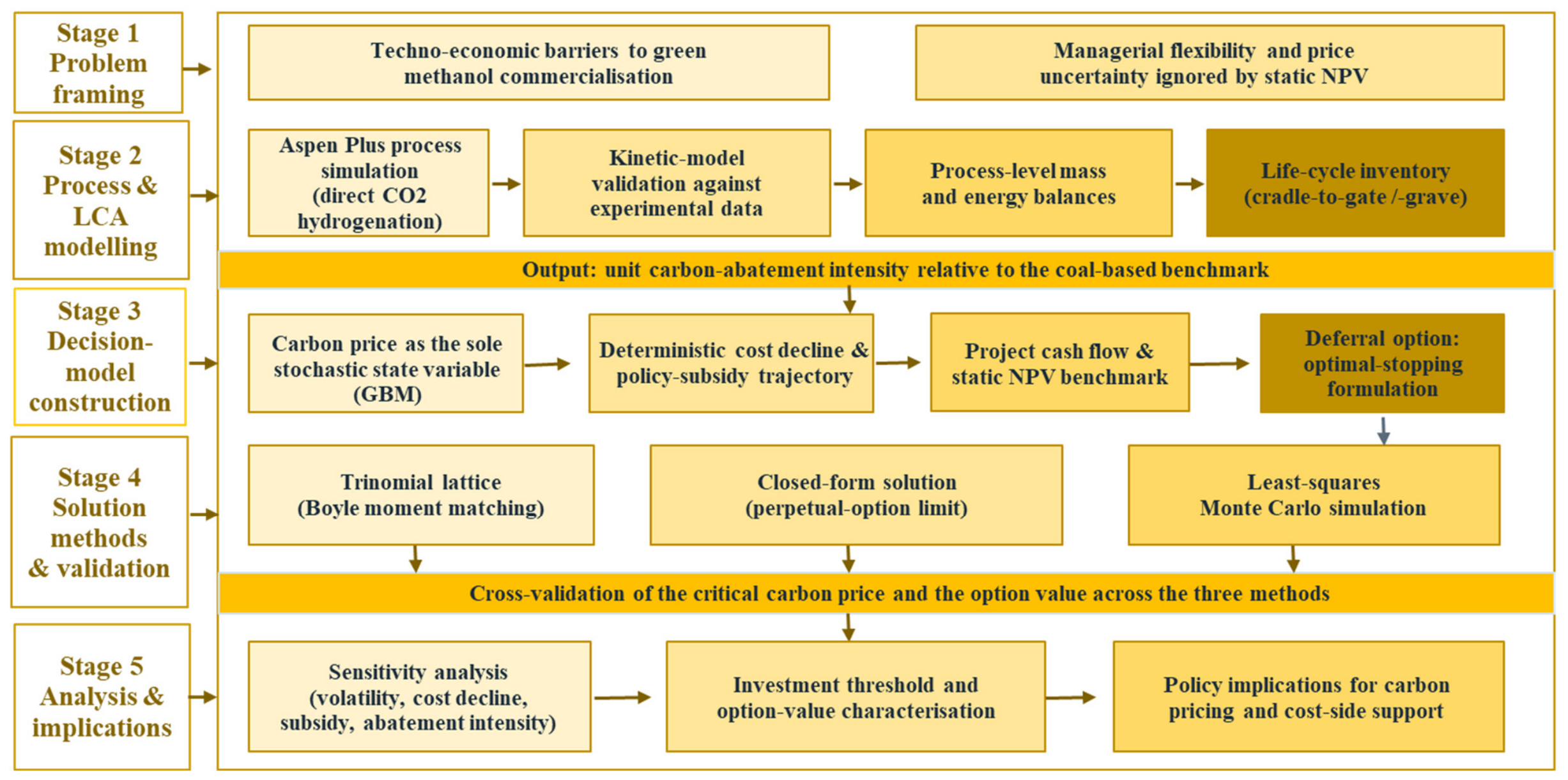
Green methanol projects are characterized by high initial investment, strong irreversibility, and long payback periods, with revenues contingent on fluctuating carbon prices. The traditional net present value (NPV) method, predicated on the rigid assumption of “invest immediately or never,” fails to capture the managerial flexibility to defer investment under uncertainty. Dixit and Pindyck [5] established that when an investment features irreversibility, uncertainty regarding future returns, and discretion over timing, real-options (RO) theory provides a more accurate valuation of a project’s intrinsic value than the NPV method. Accordingly, this section first establishes a traditional NPV model as a static evaluation benchmark. It then introduces a deferral RO framework, employing the Boyle moment-matching trinomial tree [24] to discretize the carbon price, and derives a closed-form solution for the critical carbon price to serve as a validation benchmark for the numerical algorithm.

4.1. Basic Model Assumptions

The model is built on the following core assumptions:

• Full irreversibility and decision flexibility: Once the project is implemented, sunk capital cannot be recovered; but within the investment-decision window the investor holds the flexible right (deferral option) to start the investment or to keep waiting at any discrete time point.
• Stochastic carbon price: The carbon price $P_t^C$ (defined in Section 3.6) is the core driver of revenue uncertainty. Its evolution follows a geometric Brownian motion (GBM) with drift, an assumption widely accepted and applied in low-carbon-investment real-options research [44,45,46].
• Cost-technology learning effect: The methanol product price, feedstock prices (green hydrogen, biogenic CO₂), output, and base operating costs are assumed constant over the operating period, whereas the initial investment cost and unit operating cost decline over time following a deterministic exponential trend in calendar time, a reduced-form treatment consistent with the cost-reduction paradigm of low-carbon technologies in Rubin et al. (2015) [47].
• Frictionless market: The market is assumed frictionless, with no transaction costs, tax effects, or risk-free arbitrage opportunities.
• Optimal exercise rule: When the NPV of immediate investment (intrinsic value) first becomes greater than or equal to the value of the deferral option (waiting value), the investor exercises and invests immediately; otherwise the investor keeps waiting or abandons the project.

4.2. Project Cash Flow and NPV Model

The cash-flow structure of a green methanol project is as follows. During operation, the annual net revenue consists of methanol sales revenue, the monetized value of the life-cycle abatement under the crediting scenario of Section 3.6, and the government product subsidy; the investment cost occurs at the decision point, and the actual outlay after the government investment subsidy is taken into account. The year-t net revenue is defined as

$${\mathsf{\pi }}_t=Q^{\mathrm{MeOH}}{P}^{\mathrm{MeOH}}\left(1+k\right)+\mathrm{C}\mathrm{E}{\mathrm{R}}_t{P}_t^C-C_t^{\mathrm{OM}}$$

(3)

where $Q^{\mathrm{MeOH}}$ is the annual methanol output (t/year); $P^{\mathrm{MeOH}}$ is the market price of methanol (CNY/t); k is the product-subsidy coefficient, denoting the government subsidy rate on methanol sales revenue; ${\mathrm{C}\mathrm{E}\mathrm{R}}_t$ is the carbon abatement in year t (t CO₂/year), determined by the unit abatement intensity computed in Section 3; $P_t^C$ is the carbon price in year t in the sense of Section 3.6; and $C_t^{\mathrm{O}\mathrm{M}}$ is the operating cost in year t.

The investment cost and the O&M cost are assumed to decline exponentially with calendar time:

$$C_t^I=C_0^I{e}^{-\mathsf{\alpha }t},\hspace{1em}\hspace{1em}{C}_t^{\mathrm{O}\mathrm{M}}=C_0^{\mathrm{O}\mathrm{M}}{e}^{-\mathsf{\gamma }t}$$

(4)

where $\alpha$ and $\mathsf{\gamma }$ are, respectively, the annual rate of technological change of the investment cost and of the O&M cost. The technological-learning-curve method quantifies how technology cost declines with cumulative output, knowledge capital, and scale effects, and has been widely used in cost forecasting for low-carbon technologies such as carbon capture and renewable hydrogen production [44]. Equation (4) specifies a deterministic exponential decline in unit costs with calendar time. It is a reduced-form representation of the empirically observed downward trend in low-carbon technology costs, not an endogenous learning curve: cost is not a function of cumulative output, installed capacity, or knowledge capital, and learning is therefore not endogenized to the investment decision. Endogenous-learning specifications, in which costs decline with cumulative deployment through scale and experience effects, are widely used in cost forecasting for carbon capture and renewable hydrogen [44]. We adopt the calendar-time form because a single-firm setting cannot represent industry-wide cumulative deployment, and treat the endogenous-learning extension as a priority.

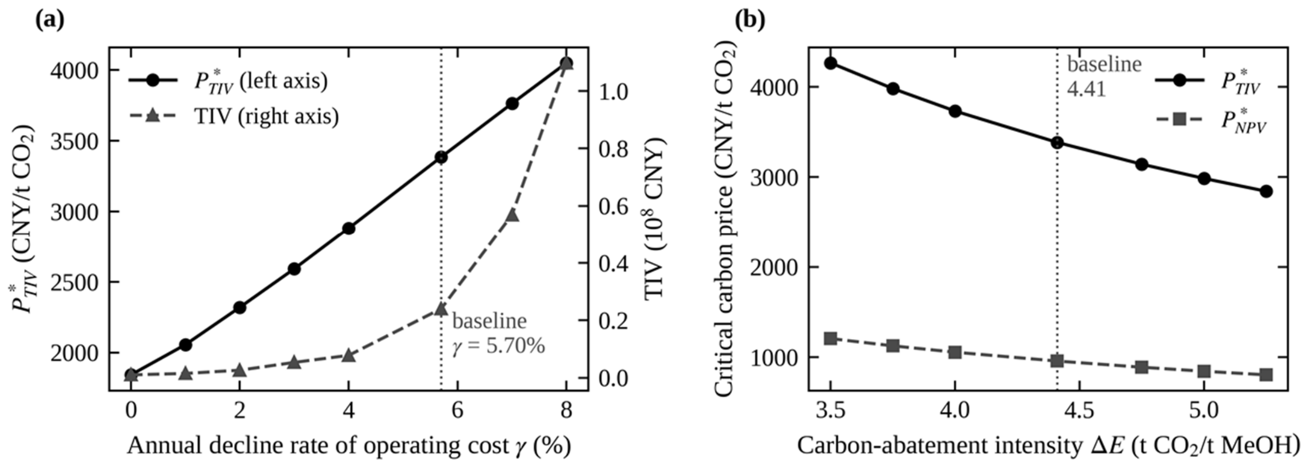
The operating cost of the plant is dominated by green hydrogen, whose delivered cost in China is projected to fall by roughly 6% to 7% per year over the coming decade [48,49]. The baseline value of γ = 5.70% per year therefore lies within the range implied by those projections rather than being assumed independently of them. Because the parameter is deterministic and dominant, it is not treated as a point estimate: Section 5.3.3 varies γ over [0, 8%], a range that spans both a static-cost scenario and a decline substantially faster than any of the cited projections, and reports the resulting range of the option value, the investment threshold and the trigger probability.

Crucially, Equations (5)–(7) evaluate the operating cost at the level prevailing on the commitment date and hold it constant in real terms over the operating period. The decline governed by $\gamma$ therefore rewards deferral of the commitment but does not continue within the operating period. This convention is used consistently in the lattice, the closed-form benchmark, and the Monte Carlo simulation, which is why the NPV of immediate investment in Section 5.3.3 is invariant to $\gamma$.

The project begins construction in the decision year, has a one-year construction period, and operates for 20 years thereafter. Using continuous-compounding discounting at a discount rate r₀, the project NPV is as follows:

$$\mathrm{NPV}\left(t_1\right)=\left[Q^{\mathrm{MeOH}}{P}^{\mathrm{MeOH}}\left(1+k\right)+\mathrm{CER}\cdot P_{t_1}^C\right]A-C_0^I\left(1-\mathsf{\lambda }\right)e^{-\mathsf{\alpha }{t}_1}-C_0^{\mathrm{O}\mathrm{M}}{e}^{-\mathsf{\gamma }{t}_1}A$$

(5)

where A is the annuity factor of the N = 20-year operating period, measured from the commitment date and therefore independent of t₁; with r₀ = 5% and N = 20, A = 11.7277. Equation (5) is stated at the commitment date, and the discounting back to date 0 is performed once, in the backward recursion of Equation (13).

$$A={\displaystyle \sum _{s=2}^{N+1}}{e}^{-r_{0}s}={\displaystyle \frac{e^{-r_0}-e^{-\left(N+1\right)r_0}}{e^{r_0}-1}}$$

(6)

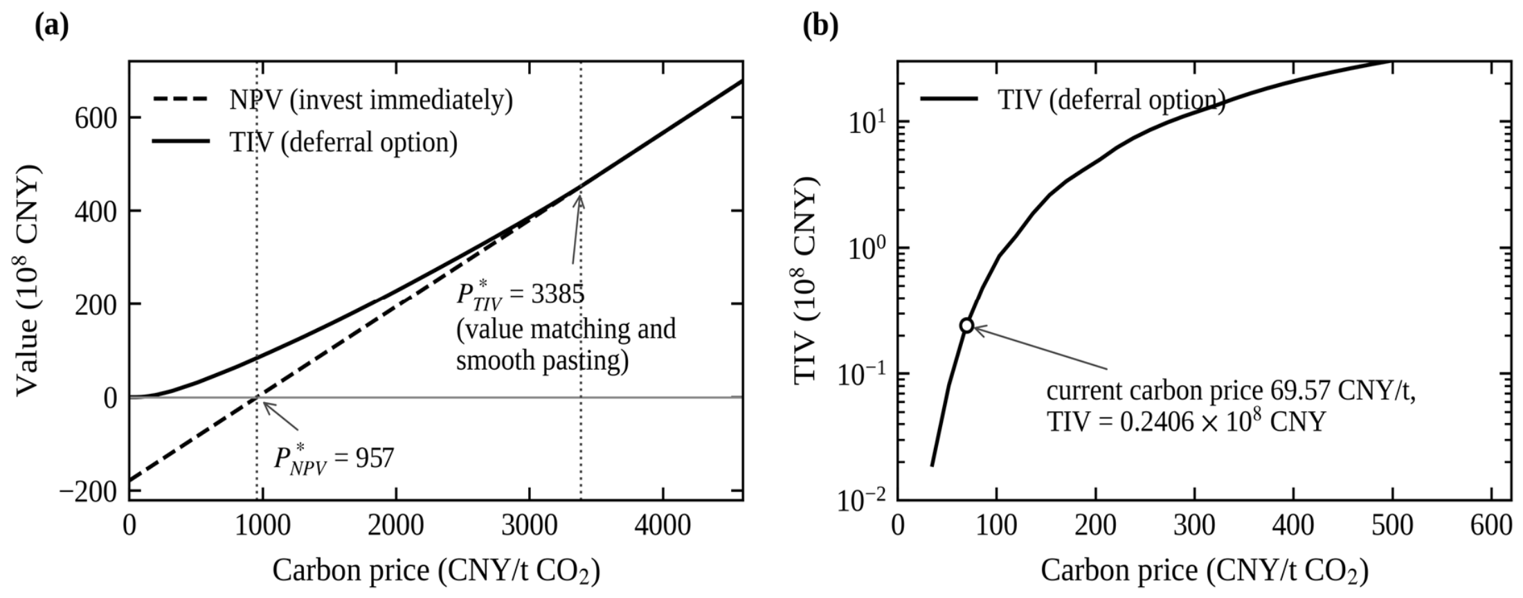
Setting NPV(t₁) = 0, the critical carbon price under the NPV method is obtained:

$$P_{\mathrm{N}\mathrm{P}\mathrm{V}}^{*} = {\displaystyle \frac{C_0^I\left(1-\mathsf{\lambda }\right)e^{-\mathsf{\alpha }{t}_1} + C_0^{\mathrm{O}\mathrm{M}}{e}^{-\mathsf{\gamma }{t}_1}A - Q^{\mathrm{M}\mathrm{e}\mathrm{O}\mathrm{H}}{P}^{\mathrm{M}\mathrm{e}\mathrm{O}\mathrm{H}}\left(1+ k\right)A}{\mathrm{C}\mathrm{E}\mathrm{R}·A}}$$

(7)

$P_{\mathrm{N}\mathrm{P}\mathrm{V}}^{*}$ denotes the minimum carbon price required for project feasibility within the static framework. Since the NPV rule is predicated on the assumption of immediate investment or abandonment, it fails to capture the value of deferral: given the right-skewed distribution of future returns, the flexibility to wait and decide contingently possesses quantifiable economic value [5]. Consequently, the real-options method is introduced.

4.3. The Stochastic Process of the Carbon Price

Empirical studies in low-carbon-investment real options at home and abroad show that the log return of the carbon price approximately follows a Gaussian process with positive drift, and that geometric Brownian motion (GBM) can effectively capture both the random fluctuation and the long-run evolution trend of the carbon price [44,48]. Its continuous-time stochastic differential equation is as follows:

$$d{P}_t^C=\mathsf{\mu }{P}_t^C\hspace{0.17em}dt+\mathsf{\sigma }{P}_t^C\hspace{0.17em}d{W}_t$$

(8)

where μ is the drift rate, denoting the expected growth rate of the carbon price; $\sigma$ is the volatility, denoting the degree of random fluctuation; and $d{W}_t$ is the increment of a standard Wiener process. To discretize the GBM and support a backward-recursive solution of the American option, this paper introduces the moment-matching trinomial-tree model proposed by Boyle (1988) [24]. Compared with the “up-down” two-state evolution of the traditional binomial tree, this model adds an intermediate “price-unchanged” state, achieving higher approximation accuracy to the continuous stochastic process for the same step size, with only linear growth in computational complexity.

Let the initial carbon price be $P_0^C$; after a step size Δt, the carbon price evolves to three states with transition probabilities $P_u$, $P_m$, and $P_d$, subject to the constraint $u·d = 1$. These probabilities are obtained by matching the first two moments of the geometric Brownian motion under the physical measure, using the drift $\mathsf{\mu }$ estimated from market data in Section 5.1; no risk-neutral drift is imposed, and no replicating portfolio is assumed. The valuation instead follows the dynamic-programming formulation of Dixit and Pindyck [5], in which all continuation values are discounted at a constant risk-adjusted rate $\rho$. Matching the two moments determines the up and down multipliers $u$, $d$ and the transition probabilities uniquely.

$$u=\exp \left(\mathsf{\sigma }\sqrt{3\Delta t}\right),d={\displaystyle \frac{1}{u}}$$

(9)

$$P_u={\displaystyle \frac{M_2+d-\left(1+d\right)M_1}{\left(u-d\right)\left(u-1\right)}}$$

(10)

$$P_d={\displaystyle \frac{M_2+u-\left(1+u\right)M_1}{\left(u-d\right)\left(1-d\right)}}$$

(11)

$$P_m=1-P_u-P_d$$

(12)

where the first moment ${ M}_1=e^{\mathsf{\mu }∆t}$, the second moment $M_2=e^{\left(2\mathsf{\mu }+{\mathsf{\sigma }}^2\right)\Delta t}$. Continuation values are discounted at $e^{-\rho \Delta t}$ in the backward recursion of Equation (13).

4.4. The Deferral Real Option and Backward Recursion

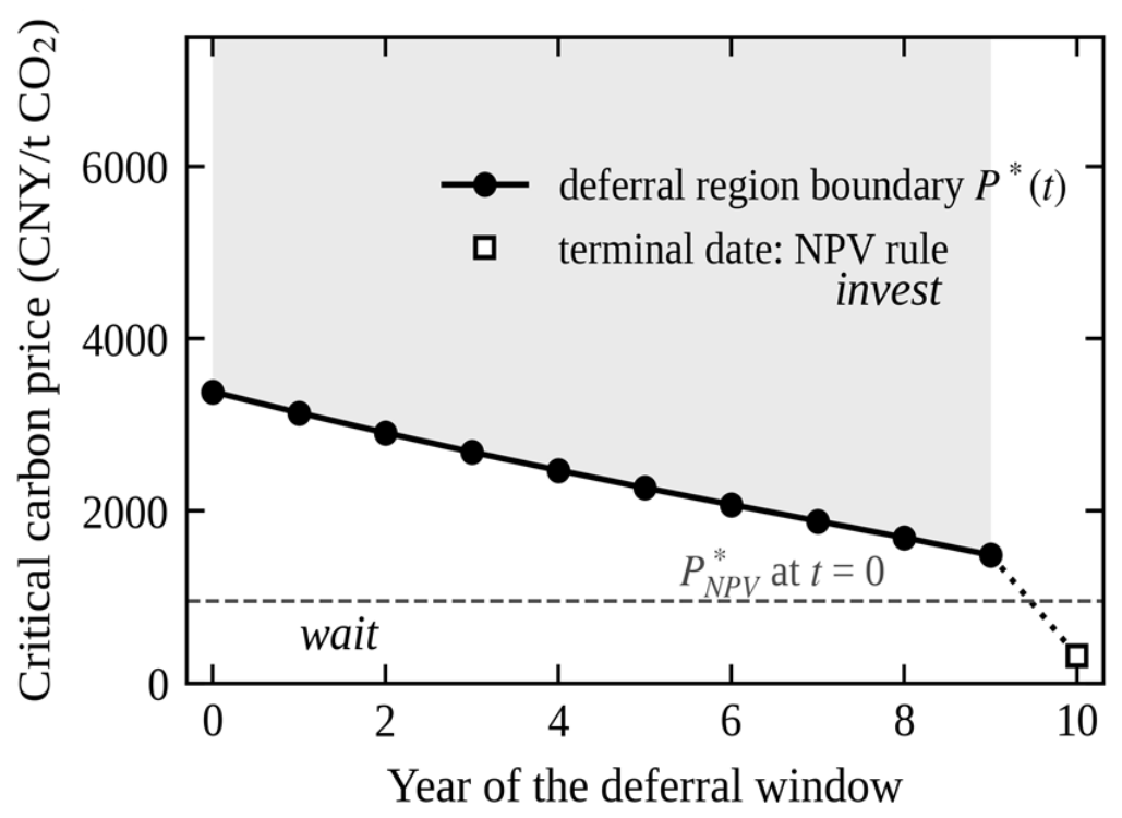
Expanding the initial carbon price along the trinomial tree over the deferral period yields the carbon price $P_{i,j}^C$ at each node (i, j) and the corresponding project NPV (${\mathrm{N}\mathrm{P}\mathrm{V}}_{i,j}$). Under the deferral-option framework, the investor at each node faces the dilemma of “invest immediately” versus “keep waiting”: if ${\mathrm{N}\mathrm{P}\mathrm{V} }_{i,j}$ < 0, immediate investment is abandoned and the node’s immediate investment value is zero; if ${\mathrm{N}\mathrm{P}\mathrm{V}}_{i,j}$ ≥ 0, the immediate investment value is ${\mathrm{N}\mathrm{P}\mathrm{V}}_{i,j}$. Recursing backward from the terminal nodes of the tree to the initial node [11,12,13], the total investment value (TIV) at each node is computed as follows:

$$\mathrm{T}\mathrm{I}{\mathrm{V}}_{i,j}=\mathrm{m}\mathrm{a}\mathrm{x}\{\mathrm{N}\mathrm{P}{\mathrm{V}}_{i,j},e^{-\rho \Delta t}\left[P_u\mathrm{T}\mathrm{I}{\mathrm{V}}_{i+1,j}+P_m\mathrm{T}\mathrm{I}{\mathrm{V}}_{i+1,j+1}+P_d\mathrm{T}\mathrm{I}{\mathrm{V}}_{i+1,j+2}\right]\}$$

(13)

Recursing back to the initial node (0, 0) yields the project’s total investment value including the option value. If and only if a node’s NPV equals its TIV does the deferral-option premium vanish and the investor become indifferent between “waiting” and “investing immediately”; the carbon price corresponding to that node is the critical carbon price under the real-options method, $P_{\mathrm{T}\mathrm{I}\mathrm{V}}^{*}$. The specific decision rules are given in

Table 6. Investment decision rules under the deferral real option.

Project NPV	Total Investment Value	Evaluation Outcome
NPV > 0	TIV > NPV	Defer investment; option premium is positive
NPV > 0	TIV = NPV	Invest immediately; option premium vanishes
NPV ≤ 0	TIV > 0	Defer investment; wait for carbon price to rise
NPV < 0	TIV ≤ 0	Abandon investment

.

4.5. Closed-Form Solution for the Critical Carbon Price and the Uncertainty Premium

Beyond the trinomial-tree numerical solution, this paper further provides an analytical expression for the critical carbon price: to reveal its intrinsic relationship with the techno-economic parameters and to offer a dual cross-validation of the numerical result. Let $V\left(P, t\right)$ be the project investment-option value function. A total-differential expansion of $V\left(P, t\right)$ by Itô’s lemma gives:

$$dV=\left[{\displaystyle \frac{\partial V}{\partial t}}+\mathsf{\mu }P{\displaystyle \frac{\partial V}{\partial P}}+{\displaystyle \frac{1}{2}}{\mathsf{\sigma }}^2{P}^2{\displaystyle \frac{{\partial }^{2}V}{\partial P^2}}\right]dt+\mathsf{\sigma }P{\displaystyle \frac{\partial V}{\partial P}}\hspace{0.17em}dz$$

(14)

The valuation follows the dynamic-programming formulation of Dixit and Pindyck [5] rather than a contingent-claims argument. Chinese carbon allowances are not fully tradable—there is no short selling and no liquid forward market—so a portfolio replicating the option payoff cannot be constructed, and imposing a risk-neutral drift on a non-traded asset with no convenience yield would drive the investment threshold to infinity and degenerate the model. We therefore retain the physical drift $\mathsf{\mu }$ and discount all continuation values at a constant risk-adjusted rate $\rho$. Because no traded replicating portfolio exists in this incomplete-market setting, the required return on the investment opportunity is not pinned down by no-arbitrage and must be supplied externally; setting $\rho$ = r₀ = 5% is accordingly an exogenous calibration choice—not a model result—adopted for parsimony. We adopt r₀ as the natural reference value and examine the sensitivity of the results to this choice in Section 5.3.1. Note that $\rho$ is a required rate of return on the investment opportunity, not the risk-free rate.

In the continuation region, the Bellman equation requires that the expected total return on holding the opportunity over an interval dt equal the required return, $\rho V\hspace{0.17em}dt=E\left[dV\right]$, where the expectation is taken under the physical measure. To obtain a closed-form benchmark, we remove the finite-horizon restriction and seek a time-independent (stationary) value function $V\left(P\right)$. 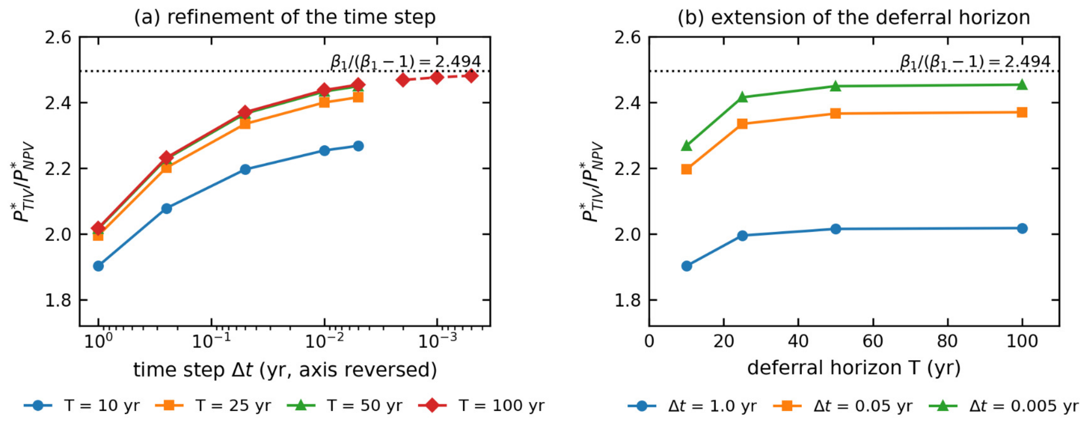This defines the perpetual problem against which the ten-year lattice is later compared in Section 5.2, and should not be read as a claim that the ten-year deferral option is itself perpetual. Since the expectation of the stochastic term vanishes, substituting Itô’s expansion and rearranging yields the second-order ordinary differential equation for the option value:

$${\displaystyle \frac{1}{2}}{\mathsf{\sigma }}^2{P}^2{\displaystyle \frac{d^{2}V}{d{P}^2}}+\mathsf{\mu }P{\displaystyle \frac{dV}{dP}}-\mathsf{\rho }V=0$$

(15)

This is an Euler–Cauchy equation. Assuming the option value function has the power form $V\left(P\right)= A·P^{\beta }$, substitution yields the characteristic equation:

$${\displaystyle \frac{1}{2}}{\mathsf{\sigma }}^2{\mathsf{\beta }}^2+\left(\mathsf{\mu }-{\displaystyle \frac{1}{2}}{\mathsf{\sigma }}^2\right)\mathsf{\beta }-\rho =0$$

(16)

This characteristic equation has one positive and one negative real root. Since the option value $V\left(P\right)$ should increase with the carbon price and tend to zero as $P$ → 0, the positive root, representing the elasticity of the upside-exercise option, is taken:

$${\mathsf{\beta }}_1={\displaystyle \frac{-\left(\mathsf{\mu }- \frac{1}{2}{\mathsf{\sigma }}^2\right) + \sqrt{{\left(\mathrm{\mu }- \frac{1}{2}{\mathrm{\sigma }}^2\right)}^2 + 2{\mathsf{\sigma }}^2\rho }}{{\mathsf{\sigma }}^2}}$$

(17)

Two conditions determine the critical carbon price: value matching, $V\left(P^{*}\right)= \mathrm{N}\mathrm{P}\mathrm{V}\left(P^{*}\right)$, and smooth pasting, $V^{\prime }\left(P^{*}\right)= {\mathrm{N}\mathrm{P}\mathrm{V}}^{\prime }\left(P^{*}\right)$. The payoff on exercise is affine in the carbon price, $\mathrm{N}\mathrm{P}\mathrm{V}\left(P\right)= \mathrm{C}\mathrm{E}\mathrm{R}·A·P - B$, where A is the annuity discount factor of Equation (6) and

$$B=C_0^I\left(1-\mathsf{\lambda }\right)e^{-\mathsf{\alpha }{t}_1}+C_0^{\mathrm{O}\mathrm{M}}{e}^{-\mathsf{\gamma }{t}_1}A-Q^{\mathrm{M}\mathrm{e}\mathrm{O}\mathrm{H}}{P}^{\mathrm{M}\mathrm{e}\mathrm{O}\mathrm{H}}\left(1+k\right)A$$

(18)

Because the payoff used in the closed-form problem is the same affine function of the carbon price that is evaluated at every node of the lattice, the two conditions solve to

$$P_{\mathrm{T}\mathrm{I}\mathrm{V}}^{*}={\displaystyle \frac{{\mathsf{\beta }}_1}{{\mathsf{\beta }}_1-1}}\cdot {\displaystyle \frac{B}{\mathrm{C}\mathrm{E}\mathrm{R}\cdot A}}={\displaystyle \frac{{\mathsf{\beta }}_1}{{\mathsf{\beta }}_1-1}}\cdot P_{\mathrm{N}\mathrm{P}\mathrm{V}}^{*}$$

(19)

If the real-options critical carbon price exceeds the NPV critical carbon price by a multiple, that multiple is the “uncertainty premium” required by the investor in the face of carbon-price uncertainty [5]:

$${\displaystyle \frac{{\mathsf{\beta }}_1}{{\mathsf{\beta }}_1-1}}>1$$

(20)

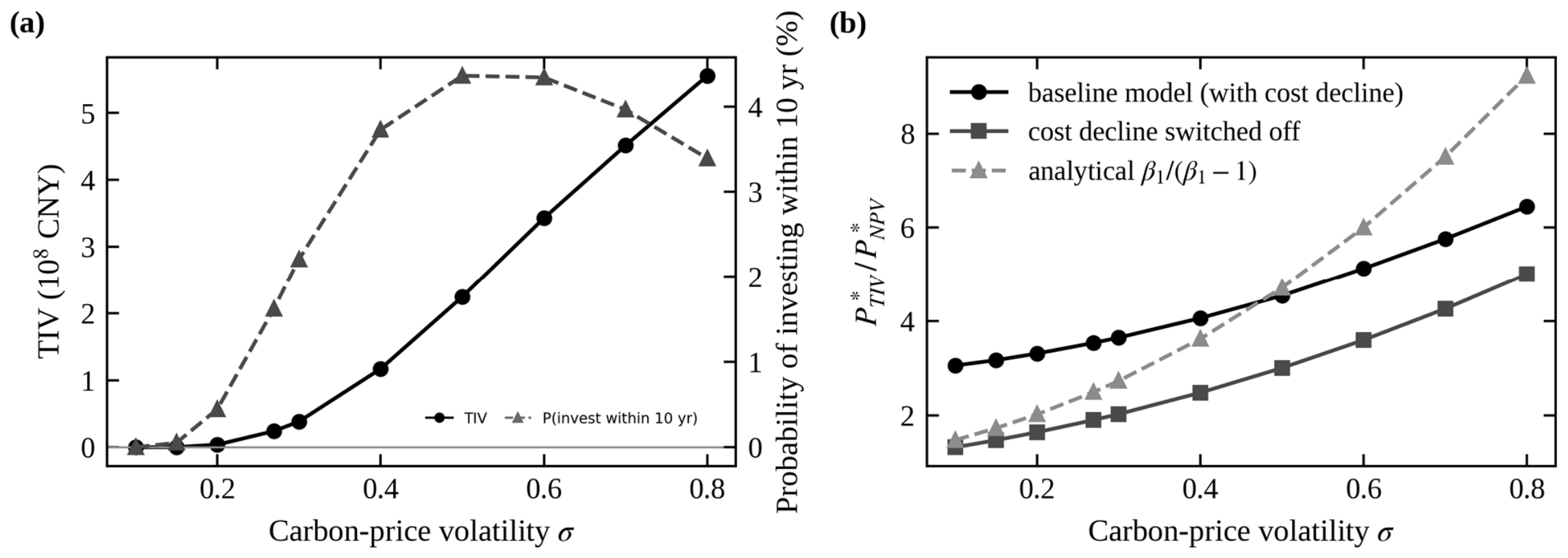
When the volatility $\sigma \to 0$, ${\mathsf{\beta }}_1\to \infty$, so that ${\displaystyle \frac{{\mathsf{\beta }}_1}{{\mathsf{\beta }}_1-1}}\to 1$, the real-options critical carbon price degenerates to the NPV critical carbon price. This degeneration is highly consistent with economic intuition—in a fully deterministic environment, “waiting” can generate no incremental information value and the value of managerial flexibility vanishes; conversely, as $\mathsf{\sigma }$ rises, ${\mathsf{\beta }}_1$ falls and the premium multiple grows correspondingly, indicating that the more violent the carbon-price fluctuation, the higher the waiting compensation the investor demands and the more prominent the strategic value of the deferral option.

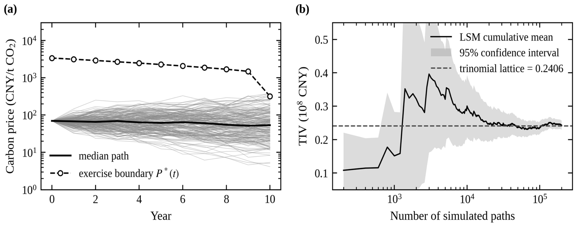
Two qualifications must be attached to Equation (19). First, it is a perpetual solution: the value function is time-independent, whereas the lattice problem imposes a ten-year deferral window, over which the exercise trigger depends on the time remaining. The two are therefore different investment problems, and the numerical closeness of two isolated figures would not validate either one. Section 5.2 accordingly verifies the closed-form result by showing that the lattice threshold converges to it as the time step is refined and the deferral horizon is extended. Second, Equation (19) is exact only when the exercise payoff is time-invariant, that is, when $\alpha = \mathsf{\gamma } = 0$; with deterministically declining costs the intercept B varies with the exercise date and no time-independent threshold exists. The closed-form expression is consequently used as a benchmark for that restricted case, while the baseline model with declining costs is solved numerically.

5. Numerical Simulation and Robustness Testing

5.1. Baseline Data and Parameter Estimation

The numerical analysis is based on a 360,000 t/yr demonstration project for the direct hydrogenation of CO₂ to methanol. Baseline parameters are categorized into technical, economic, carbon-emission, and carbon-price groups (

Table 7. Summary of baseline parameters for the numerical simulation.

Category	Parameter	Symbol	Value	Unit/note
Technical	Annual methanol output	Q	36	104 t/year
	CO2 unit consumption	-	1.42	t/t MeOH (Aspen)
	H2 unit consumption	-	0.196	t/t MeOH (Aspen)
	Project life	t2 − t1	20	years
Economic	Initial investment	C0ᴵ	141,290	104 CNY
	Annual operating cost	C0ᴼᴹ	228,352	104 CNY/year
	Methanol market price	$P^{\mathrm{M}\mathrm{e}\mathrm{O}\mathrm{H}}$	2458	CNY/t (Wind 5-yr mean)
	Discount rate	$\rho =r_0$	5	%
	Investment-cost change rate	α	2.02	%
	O&M-cost change rate	γ	5.70	%
Carbon emission and price	Unit abatement intensity	ΔE	4.41	t CO2/t MeOH
	Annual carbon abatement	CER	158.76	104 t CO2/year
	Baseline carbon price	P0ᶜ	69.57	CNY/t (Wind)
	Drift rate μ	μ	0.0057	—
	Volatility σ	σ	0.2692	—

). Technical parameters derive from the Aspen Plus simulation (Section 3), while the 20-year operating life—commencing after a one-year construction period—follows industry depreciation norms. The initial investment is scaled from the Ordos 100,000 t/yr project [49] (exponent = 0.65). Operating costs, dominated by green hydrogen, include feedstocks and utilities, and the methanol price is the five-year national average (Wind database). Carbon-emission data are drawn from Section 3.

The parameters of the carbon-price stochastic process are estimated from the daily closing-price series of China’s national carbon emissions-trading market (CEA) from 16 July 2021 to 16 July 2025. The log-return series of the carbon price is first computed and annualized at 240 trading days per year, yielding the annualized drift and volatility (see Table 7). Substituting these parameters together with the risk-adjusted discount rate ρ and the step size Δt, into Equations (9)–(12) yields the up and down multipliers u = 1.5940 and d = 0.6273.

5.2. Baseline Scenario: Investment Value and the Critical Carbon Price

Under the baseline scenario without government subsidies ($k=\mathsf{\lambda }=0$), the analysis covers a deferral period of 0–10 years. The trinomial tree is expanded from an initial carbon price of 69.57 CNY/t to map price paths at each node. The project NPV is calculated using Equation (5), and the total investment value (TIV) is derived via backward recursion using Equation (13). Figure 2 illustrates the evolution of NPV and TIV along the baseline, highest, and lowest paths over the deferral horizon.

Figure 2 illustrates the underlying dynamics. Panel (a) depicts the two value functions against the current carbon price. The NPV of immediate investment is linear, crossing zero at $P_{\mathrm{N}\mathrm{P}\mathrm{V}}^{*}$ = 956.9 CNY/t. The TIV remains strictly above the NPV, bounded below by zero, and meets it tangentially at $P_{\mathrm{T}\mathrm{I}\mathrm{V}}^{*}$ = 3384.7 CNY/t. At this point, the value-matching and smooth-pasting conditions are satisfied, signifying that the option premium is fully dissipated. Panel (b) presents a magnified view of the region around the current carbon price on a logarithmic scale. The option value at 69.57 CNY/t is positive but negligible, falling three orders of magnitude below the project’s scale. It rises sharply only as the carbon price approaches several hundred CNY/t. Thus, the economic essence of the deferral option in this project is the avoidance of an irreversible commitment under adverse conditions, rather than the prospect of a large upside gain.

The ratio of the two critical carbon prices is calculated to be 3.54. This figure should not be directly equated to the closed-form multiple ${\displaystyle \frac{{\mathsf{\beta }}_1}{{\mathsf{\beta }}_1-1}}=2.4941$ obtained from Equation (17), as they represent distinct analytical frameworks. Specifically, the lattice model solves a ten-year, annually exercisable option with deterministically declining costs, whereas Equation (19) describes a perpetual, continuously exercisable option with time-invariant costs.

Table 8. Decomposition of the real-options threshold.

Specification	${\mathit{P}}_{\mathbf{T}\mathbf{I}\mathbf{V}}^{\mathsf{*}}$ (CNY/t CO2)	${\mathit{P}}_{\mathbf{T}\mathbf{I}\mathbf{V}}^{\mathsf{*}}$/${\mathit{P}}_{\mathbf{N}\mathbf{P}\mathbf{V}}^{\mathsf{*}}$
T = 10 yr, annual decisions, no cost decline	1820.4	1.902
T = 10 yr, dt = 0.005 yr, no cost decline	2170.1	2.268
T -> inf, dt -> 0, no cost decline (analytical)	2386.5	2.494
T = 10 yr, annual decisions, with cost decline	3384.7	3.537
T = 10 yr, dt = 0.005 yr, with cost decline	3993.3	4.173

decomposes the contributing factors. With cost-decline parameters deactivated, the ten-year lattice yields a ratio of 1.90. Two distinct sources of discrepancy separate this figure from the analytical multiple of 2.494, and they must be relaxed jointly rather than in isolation. Refining the time step alone, at a fixed ten-year horizon, cannot make a finite-horizon option equal to a perpetual one: the ratio rises to 2.268 at Δt = 0.005 yr and then saturates, the residual gap being the value of the exercise opportunities beyond year ten. Conversely, extending the horizon alone at annual decision dates saturates at 2.018, the residual gap being the value of the exercise opportunities forgone between decision dates. Only when both limits are taken together does the lattice approach the analytical value. Figure 3 reports this joint convergence.

Figure 4 reports the finite-horizon exercise boundary. This boundary declines monotonically from 3384.7 CNY/t at t = 0 to 1488 CNY/t at t = 9, reflecting that declining capital and operating costs allow project viability at progressively lower carbon prices. At the terminal date, the option to wait expires, and the decision reverts to the static NPV test, causing the boundary to drop discontinuously to 318 CNY/t. The exercise boundary further contextualizes the baseline results. Simulating the estimated carbon-price process against the boundary in Figure 4 yields a mere 1.60% probability of investment triggering within the ten-year window, with conditional investment occurring almost exclusively at the terminal date. Thus, the baseline scenario implies that waiting for the carbon price to reach 3384.7 CNY/t is highly improbable; rather, immediate investment is suboptimal. The decision should be revisited at the window’s end against a threshold near 318 CNY/t. Absent additional policy support or cost reductions, the project is unlikely to become attractive within the decision horizon.

5.3. Sensitivity Analysis

5.3.1. Carbon-Price Volatility

Carbon-price volatility $\mathsf{\sigma }$ is the core parameter characterizing the uncertainty of the carbon value defined in Section 3.6; its magnitude directly affects the investor’s judgment of the deferral-option value and the setting of the critical investment threshold. This section sets the range of $\mathsf{\sigma }$ to [0.10, 0.80], covering the full spectrum from low to extremely high volatility, with $\mathsf{\sigma }= 0.2692$ being the baseline value estimated from CEA historical daily closing prices. The simulation results are shown in Figure 5.

Two features merit attention. First, Panel (b) demonstrates that the baseline ratio ${\displaystyle \frac{P_{TIV}^{*}}{P_{NPV}^{*}}}$ does not converge to unity as σ declines; instead, it asymptotes near 3.06. This residual premium reflects the deterministic incentive to wait for cheaper technology, which operates independently of uncertainty. Conversely, with cost-decline terms removed, the ratio tracks the analytical multiple. Second, the probability of investment within ten years exhibits a hump-shaped relationship with σ: it rises from negligible levels at $\mathsf{\sigma }=0.10$ to a peak of roughly 4.4% at $\mathsf{\sigma }=0.5-0.6$, before declining to 3.4% at $\mathsf{\sigma }=0.80$. While higher volatility increases the likelihood of reaching a high carbon price, it simultaneously raises the investment threshold; eventually, the latter effect dominates. Consequently, higher volatility enhances the value of the investment opportunity without necessarily increasing the likelihood of execution—a nuance that the option value alone fails to reveal.

5.3.2. Product Subsidy Versus Investment Subsidy

We evaluate two policy instruments: a product subsidy applied at rate $k$ to methanol sales revenue over the operating period, and an investment subsidy applied at rate $\mathsf{\lambda }$ to the initial capital outlay. While both instruments improve project economics monotonically, they cannot be meaningfully compared at equal coefficients, as they apply to distinct monetary bases and operate over different time horizons. Evaluated at the project discount rate, $k=1$ corresponds to a present value of government expenditure of 10,378 million CNY, whereas $\mathsf{\lambda }=1$ corresponds to 1413 million CNY. Consequently, a comparison of $k=1$ with $\mathsf{\lambda }=1$ contrasts fiscal commitments that differ by a factor of 7.3; any ratio of effects derived from such a comparison largely reflects this discrepancy rather than measuring incentive efficiency. We therefore compare the two instruments based on an equal present value of government expenditure. Setting the budget at 1413 million CNY—which exhausts the investment subsidy at $\mathsf{\lambda }=1$—yields a fiscally equivalent product subsidy rate of k = 0.1361.

The results differ significantly from those obtained via a comparison at equal coefficients. At equal fiscal cost, the improvement in net present value (NPV) is identical for both instruments (1413 million CNY), which is not a coincidence: NPV is linear in each subsidy, so a transfer of a given present value passes through unit-for-unit regardless of form. The static criterion is therefore insufficient for ranking the two instruments. Differences emerge only in the option dimension and are modest in magnitude. The product subsidy raises the total investment value (TIV) to 46.36 million CNY against 40.07 million CNY for the investment subsidy, and increases the probability of investment within ten years to 3.39% versus 2.93%; thus, on these two criteria, it is approximately 1.16 times as effective. However, regarding the reduction in the current-date critical carbon price, the investment subsidy performs slightly better, lowering it to 3232.0 CNY/t compared to 3270.3 CNY/t for the product subsidy. This occurs because the investment subsidy targets the fixed-cost component of the exercise payoff, which is not scaled by the operating-period annuity factor.

At comparable fiscal costs, the two instruments are thus broadly equivalent, with the ranking dependent on the adopted criterion. Only when the budget is sufficiently large for the investment subsidy to saturate at $\mathsf{\lambda }=1$ does the product subsidy become clearly superior, as the capital-side instrument can absorb no further expenditure (Figure 6). The policy implication is not that operating-period support should be the primary instrument, but rather that the choice between the two should be governed by the program size and the specific margin the policymaker intends to influence. Claims of large efficiency differences between subsidy instruments should be treated with caution unless they are established at a common fiscal cost.

5.3.3. The Rate of Decline in Operating Costs

The annual operating cost of 2284 million CNY exceeds the initial capital investment of 1413 million CNY and is dominated by the cost of green hydrogen. We assume this cost declines at a rate of $\mathsf{\gamma }=5.70\%$ per year in calendar time. Given that a deterministic decline of this magnitude, sustained over two decades, constitutes a compelling rationale for delaying investment, $\mathsf{\gamma }$ warrants explicit sensitivity analysis. We examine the sensitivity by varying $\mathsf{\gamma }$ over the interval [0, 8%] (Figure 7a).

While the net present value (NPV) of immediate investment remains unaffected—being evaluated at the date-0 cost level—the option value and the investment threshold demonstrate heightened sensitivity to this parameter. As $\mathsf{\gamma }$ increases from 0 to 8%, the total investment value (TIV) rises from 1.02 million to 109.78 million CNY, the critical carbon price increases from 1843 to 4049 CNY/t, and the probability of investment within ten years grows from 0.03% to 10.2%. Thus, the rate of decline in operating costs acts as the single most potent driver of investment timing in this model—exerting greater influence than carbon-price volatility over any plausible range. Consequently, results conditional on $\gamma$ must be interpreted with this sensitivity in mind.

This finding also necessitates a clarification of terminology. Equation (4) models costs as declining exponentially with calendar time. This represents a deterministic time trend rather than an endogenous learning curve driven by cumulative deployment, and it is treated as such throughout this study. A structural learning specification—where cost reductions are driven by cumulative installed capacity and are thus partially endogenous to the investment decision—would alter timing incentives in two opposing directions. It would weaken the incentive to wait, as deferral by all firms slows the very cost decline being awaited, while introducing a strategic incentive to invest early to influence the industry learning path. Capturing this endogeneity requires an equilibrium framework beyond the single-firm setting adopted here, and is identified in Section 7.2 as a priority extension.

5.3.4. Carbon-Abatement Intensity

The unit abatement intensity $\Delta E$, scales the carbon revenue multiplicatively in the payoff function, thereby exerting an inverse influence on the critical carbon price. As detailed in Section 3.5, $\Delta E$ is sensitive to both the coal-based benchmark, which the literature places between 4.06 and 6.50 kg CO₂eq/kg on a matched boundary, and the energy supply assumptions for the green methanol plant. Consequently, we evaluate the model over a $\Delta E$ range of [3.00, 5.25] t CO₂/t MeOH (Figure 6b) rather than treating it as a fixed parameter. Within this interval, $P_{\mathrm{N}\mathrm{P}\mathrm{V}}^{*}$ declines from 1407 to 844 CNY/t and ${P^{*}}_{\mathrm{T}\mathrm{I}\mathrm{V}}$ from 4975 to 2985 CNY/t, while the probability of investment within ten years increases from 0.48% to 2.32%. Although the qualitative conclusion remains robust—the project lacks economic viability across the entire spectrum—the quantitative thresholds are contingent on the abatement benchmark and should be interpreted with this associated uncertainty.

5.3.5. Sensitivity to the Risk-Adjusted Discount Rate

The required return on the investment opportunity, $\rho$, is not pinned down by no-arbitrage in this incomplete-market setting and is calibrated exogenously as $\rho$ = r₀ = 5%.

Table 9. Sensitivity of the baseline results to the risk-adjusted discount rate.

$\mathit{\rho }$	${\mathsf{\beta }}_{\mathbf{1}}$	$\frac{{\mathsf{\beta }}_{\mathbf{1}}}{{\mathsf{\beta }}_{\mathbf{1}}-\mathbf{1}}$	${{\mathit{P}}^{\mathsf{*}}}_{\mathbf{N}\mathbf{P}\mathbf{V}}$ (CNY/t)	${{\mathit{P}}^{\mathsf{*}}}_{\mathbf{T}\mathbf{I}\mathbf{V}}$ (CNY/t)	Ratio	TIV (×108 CNY)	Pperp (CNY/t)	P (≤10 yr)
4%	1.5534	2.807	949.6	4068.2	4.28	0.3025	2665.7	1.69%
5%	1.6693	2.494	956.9	3384.7	3.54	0.2406	2386.5	1.60%
6%	1.7754	2.290	964.6	2957.8	3.07	0.1913	2208.6	1.51%
7%	1.8737	2.145	972.8	2666.4	2.74	0.1521	2086.3	1.42%
8%	1.9658	2.035	981.6	2456.0	2.50	0.1210	1997.9	1.33%

reports the sensitivity of the baseline results to $\rho$ over [4%, 8%]. Both the option value and the threshold premium decline monotonically as $\rho$ rises, because a higher required return discounts the payoff to deferral more heavily: the analytical perpetual multiple ${\displaystyle \frac{{\mathsf{\beta }}^1}{{\mathsf{\beta }}^1-1}}$ falls from 2.81 at $\rho$ = 4% to 2.04 at $\rho$ = 8%, the threshold premium falls from 4.28 to 2.50 times the static level, and the ten-year trigger probability stays below 2% throughout, while the static threshold ${P^{*}}_{\mathrm{N}\mathrm{P}\mathrm{V}}$ is nearly invariant (949.6–981.6 CNY/t). The baseline conclusions—a threshold several times the NPV level, a positive but small option value, and a low probability of investment within the deferral window—are qualitatively unchanged across this range and are therefore not artefacts of the specific value $\rho$ = 5%. As a complementary check that isolates the equality $\rho$ = r₀ holding r₀ fixed at 5% and varying only $\rho$ yields the same qualitative picture, with ${P^{*}}_{\mathrm{T}\mathrm{I}\mathrm{V}}$ moving between 4085 and 2414 CNY/t and the trigger probability essentially unchanged (about 1.6%), which is dominated by the terminal-date decision governed by r₀.

5.4. Monte Carlo Cross-Validation

The deferral option evaluated is of the American style, implying that the continuation value at an intermediate decision date represents a conditional expectation based on the information available at that time. This value cannot be recovered from the subsequent realization of a single simulated path, as doing so would endow the investor with perfect foresight. Therefore, we value the option using the least-squares Monte Carlo method developed by Longstaff and Schwartz [26].

The simulation parameters strictly follow Section 5.1 to ensure comparability: initial carbon price $P_0^C$ = 69.57 CNY/t, annualized drift $\mathsf{\mu }$ = 0.0057, annualized volatility $\mathsf{\sigma }$ = 0.2692 (strictly identical to the trinomial-tree model), step size Δt = 1 year, deferral period T = 10 years, and number of paths N = 10,000; the project fundamentals match the baseline scenario ($k = \mathsf{\lambda } = 0$). The carbon-price paths are generated using the exact Itô discretization form:

$$P_{t+1}^C=P_t^C\mathrm{e}\mathrm{x}\mathrm{p}\left[\left(\mathsf{\mu }-{\displaystyle \frac{1}{2}}{\mathsf{\sigma }}^2\right)\Delta t+\mathsf{\sigma }\sqrt{\Delta t}\hspace{0.17em}{\mathsf{\epsilon }}_t\right]$$

(21)

At each decision date t = 9, …, 1, the continuation value is estimated by regressing the discounted realized continuation values on the basis {1, Pt, Pt2} across the paths that are in the money (i.e., those with a positive immediate investment value). Investment is triggered at the earliest date where the immediate investment value exceeds the fitted continuation value, and the discounted cash flows are averaged over all paths.

Because the option is deeply out-of-the-money at the baseline carbon price, the estimator is dominated by a small fraction of paths, necessitating a large sample size. With 10,000 paths, the standard error is 4.0 million CNY, approximately 16% of the estimate. However, with 4 × 10⁶ antithetic paths, the estimate converges to 24.18 million CNY with a standard error of 0.15 million CNY. This compares favorably with the 24.06 million CNY derived from the trinomial lattice—a difference of merely 0.5%, which lies within one standard error. Since both procedures value the same option under the same probability measure and exercise rule, this agreement constitutes genuine cross-validation rather than a numerical coincidence. It is important to note that the confidence interval reflects sampling uncertainty conditional on the simulation model and does not, by itself, establish equivalence between the two valuation procedures.

For comparative purposes, applying backward induction independently along each simulated path—effectively treating the realized path as known to the investor at every decision date—yields a value of 28.02 million CNY on the same sample. The 16.5% upward bias observed is the perfect-foresight bias that the least-squares regression is specifically designed to eliminate; this illustrates why path-wise recursion is not an admissible method for valuing American-style options.

Figure 8a visualizes 200 of the simulated paths on a logarithmic scale alongside the exercise boundary. The paths diffuse symmetrically in logarithms, consistent with the lognormal property of the process. The visual separation between the bulk of the distribution and the boundary provides a direct illustration of the low trigger probability reported in Section 5.2: the option derives its value exclusively from a thin right tail of trajectories. Panel (b) illustrates the convergence of the least-squares Monte Carlo estimate.

6. Discussion

The results presented in this study diverge significantly from the comparable literature, necessitating a careful decomposition of the underlying drivers. Rather than merely reporting numerical discrepancies, we identify three core dimensions—economic configuration, uncertainty mechanisms, and methodological rigor—that contextualize our findings and validate the analytical framework.

6.1. Sources of Threshold Divergence

The substantial difference between our investment threshold and those of existing studies, such as Fu et al. [22], stems primarily from project configuration rather than option methodology. First, our baseline calibration is validated against static techno-economic literature: our break-even methanol price (6371 CNY/t) lies between the estimates of Zhang Xuan et al. [3] and Liu Jian et al. [4], and our static break-even carbon price (956.9 CNY/t) is consistent with the cost structures reported by Pérez-Fortes et al. [11]. Second, the gap relative to Fu et al. [22] is largely due to the boundary of analysis. While Fu et al. model a retrofit at an integrated site where CO₂ and hydrogen are marginal by-products, we model a greenfield plant purchasing electrolytic hydrogen at market prices. Consequently, our operating costs (2284 million CNY/year) dominate the economics, requiring a significantly higher carbon price to cover the operating deficit before capital recovery. Third, our investment threshold is elevated by deterministic cost declines. When isolating the pure uncertainty premium (by removing cost-decline terms), the threshold ratio aligns closely with theoretical multiples. Finally, the accounting of abatement intensity significantly impacts the threshold; variation in system boundaries and biogenic carbon treatment, as seen in comparisons with Liu Jian et al. [4], can shift the economic conclusion by a factor of 1.7. Thus, thresholds are not portable across studies without explicit documentation of configuration and accounting conventions.

6.2. The Dual Nature of Uncertainty

Our analysis refines the understanding of how carbon-price volatility affects investment. Confirming the findings of Gong Piqin and Li Xinyang [9], we observe that higher volatility raises the investment threshold. However, by explicitly calculating the trigger probability, we reveal a non-monotonic relationship: probability increases with volatility up to a point ($\mathsf{\sigma }$ ≈ 0.5–0.6) but decreases thereafter. This indicates that while uncertainty increases the value of the investment option, it simultaneously raises the hurdle for execution. Consequently, a more volatile carbon market may make the project option more valuable while making actual investment less likely. Furthermore, this dynamic has a policy implication: frequently revised subsidy regimes increase effective volatility, thereby raising the investment threshold and partially offsetting the subsidy’s intended benefit. A stable, pre-announced policy path can compress this uncertainty premium at no additional fiscal cost.

6.3. Methodological Verification and Robustness

This study contributes a rigorous cross-validation framework for real options in emerging markets. Agreement between numerical methods is treated as evidence only when they value the same option under identical measures and exercise rules. We therefore impose convergence tests rather than comparisons of isolated figures. The lattice solution approaches the closed-form perpetual multiple β₁/(β₁ − 1) = 2.4941 only when the two restrictions that separate the two problems are relaxed jointly: refining the time step at a fixed ten-year horizon saturates at 2.268, and extending the horizon at annual decision dates saturates at 2.018, whereas taking both limits together (Δt → 0 and T → ∞) carries the lattice ratio to 2.481. The least-squares Monte Carlo (LSM) estimate of 24.18 million CNY likewise aligns with the lattice value of 24.06 million CNY to within one standard error. It is this convergence, rather than mere numerical proximity, that validates the model. We also demonstrate that naive path-wise recursion carries a significant upward bias (16.5%), highlighting the necessity of LSM for American-style options. The consistent reporting of the finite-horizon exercise boundary, rather than a single trigger price, further enhances the transparency of the investment timing logic.

7. Conclusions and Policy Recommendations

7.1. Research Conclusions

Driven by the “dual-carbon” goals, green methanol represents a critical pathway for the deep decarbonization of the chemical and hard-to-abate sectors; however, its commercialization is constrained by high green-hydrogen costs, policy dependencies, and the volatility of carbon price. This study establishes an investment-timing framework that couples Aspen Plus process simulation with real-options analysis (ROA), validated through a rigorous dynamic-programming approach involving trinomial lattices, closed-form solutions, and least-squares Monte Carlo simulation. Applied to the demonstration project in China, the analysis yields the following conclusions:

First, the static NPV rule does not capture the value of retaining the option to wait and therefore misprices the investment opportunity rather than merely rejecting it. At the current carbon price, immediate investment yields an NPV of approximately –16.5 billion CNY and would be rejected under the static criterion; yet this does not mean the project is viable today. Under the baseline calibration, the probability of investment being triggered within the ten-year window is only 1.60% without additional policy support or further cost reductions, the project is unlikely to become attractive within that horizon. What the real-options framework adds is a positive option value of 24.1 million CNY attached to the flexibility of deferral—waiting and investing contingently rather than committing or abandoning today. The real-options critical carbon price (3384.7 CNY/t) exceeds the static threshold (956.9 CNY/t) by a factor of 3.5. By forcing an immediate invest-or-abandon choice, static appraisal discards this value of waiting entirely. These findings are also robust to the calibration of the risk-adjusted discount rate ρ: over the plausible range [4%, 8%], the threshold premium remains above 2.5 times the static level, the option value stays positive but small, and the ten-year trigger probability remains below 2%.

Second, the gap between the real-options and static-NPV thresholds is driven by both carbon-price uncertainty and the assumed deterministic decline in operating costs. When the cost-decline component is removed, the uncertainty-related threshold multiple converges to the perpetual benchmark of 2.49. The remaining increase reflects the benefit of waiting for lower future operating costs, which are dominated by green-hydrogen costs in the baseline setting. Furthermore, the sensitivity analysis shows that the operating-cost decline rate has a stronger effect on investment timing than carbon-price volatility over the examined ranges. Accordingly, policies that stabilize the carbon market can reduce only the uncertainty-related component of the investment barrier.

Third, carbon-price volatility has different implications for option value and for investment occurrence. Higher volatility raises both the option value and the investment threshold, but its effect on the ten-year trigger probability is non-monotonic: the probability first rises at moderate volatility and then falls once the exercise boundary recedes faster than prices are likely to reach it. A more volatile carbon market can thus increase the value of waiting while making actual investment less likely—an outcome that argues for stable and predictable policy conditions.

Fourth, product and investment subsidies are broadly similar in effectiveness when compared at equal present values of government expenditure. Under this fiscally comparable basis, the product subsidy is modestly more effective (by approximately 16%) in raising option value and the probability of investment, whereas the investment subsidy marginally lowers the immediate exercise threshold. The choice between these instruments should therefore also consider the scale, timing, and administrative feasibility of the policy program, rather than presume a large intrinsic efficiency difference.

7.2. Policy Implications and Future Outlook

The findings indicate that carbon pricing alone is unlikely to trigger investment in the representative green-methanol project within the ten-year decision horizon under the baseline calibration. Measures that improve green-hydrogen affordability and reduce operating costs are therefore central to improving investment prospects, as the assumed cost decline dominates carbon-price volatility in shaping the timing decision. Because product and investment subsidies perform broadly similarly when benchmarked at equal present values of fiscal expenditure, the choice between them should rest on program scale, timing, and administrative feasibility rather than on presumed efficiency differences. Policymakers should also provide stable, pre-announced policy paths: greater uncertainty raises the value of waiting and, beyond moderate levels, makes actual investment less likely, so predictability in the policy environment matters for timing as much as the level of support.

These quantitative results are conditional on the deterministic operating-cost decline, the carbon-abatement accounting boundary, and the single-firm decision setting; the required-return calibration, by contrast, affects none of the qualitative conclusions over the plausible range examined. Future research should therefore model endogenous learning driven by cumulative deployment—capture of which requires an equilibrium framework beyond the single-firm setting adopted here—and treat the availability of compliant carbon-credit methodologies as an explicit stochastic state variable.