Enhancing Long-Term Forecasting Stability in Smart Grids: A Hybrid Mamba-LSTM-Attention Framework

Abstract

Accurate multivariate long-term time series forecasting (LTSF) is critical for smart grid operations. However, non-stationary distribution shifts frequently induce compounding error accumulation in conventional architectures. This study proposes the Mamba-LSTM-Attention (MLA) framework, a distribution-aware architecture engineered for forecasting stability. The pipeline integrates Reversible Instance Normalization (RevIN) to neutralize statistical drift. To address computational bottlenecks, the architecture utilizes a linear-time Selective State Space Model (Mamba) to capture global trend dynamics, cascaded with a single-layer gated Long Short-Term Memory (LSTM) unit to model localized non-linear residuals. A terminal information bottleneck structurally bounds cross-step error propagation. Empirical results across standard ETT and Electricity benchmarks reveal a precision–stability trade-off. By prioritizing structural resilience, the MLA framework limits error accumulation on highly volatile datasets, yielding MSEs of 0.210 and 0.128 on ETTh2 and ETTm2 at the T = 96 horizon. This structural bottleneck inherently smooths high-frequency periodic patterns, yielding lower absolute accuracy on stationary benchmarks such as ETTh1 and ETTm1. Ultimately, the architecture establishes a computationally efficient, structurally stable baseline tailored for non-stationary anomaly tracking in smart grids.

1. Introduction

Accurate multivariate Long-Term Time Series Forecasting (LTSF) remains a critical operational prerequisite for dynamic peak-shaving, anomaly detection, and reliable energy dispatch in modern smart grids [1]. As industrial data acquisition scales, predictive models are increasingly mandated to decode deep periodicities across extended forecasting horizons. However, real-world electrical load sequences are frequently disrupted by extreme meteorological events and sudden socioeconomic fluctuations, resulting in substantial non-stationary distribution shifts [2,3,4,5]. This temporal and feature-level volatility imposes significant demands on the structural robustness of predictive architectures. Conventional recurrent networks and early deep learning paradigms inherently exhibit receptive field decay and cascading autoregressive error accumulation when confronted with such out-of-distribution anomalous load spikes, making them unsuitable for stable long-term grid monitoring [6,7]. Beyond macro-level grid dispatching, precise load forecasting directly impacts the operational integrity of critical infrastructure, particularly power transformers. Anomalous load spikes induce substantial thermal and mechanical stresses, significantly accelerating internal insulation degradation. Consequently, robust predictive models are essential to proactively monitor equipment conditions, prevent sustained overloading, and avert system-wide hardware failures [8].

While Transformer-based architectures have emerged as the dominant paradigm by expanding the global receptive field through self-attention mechanisms [9,10], their quadratic computational complexity $\left(O\right(L^2\left)\right)$ introduces substantial memory bottlenecks during extended historical look-backs [11,12,13,14]. Furthermore, recent dominant strategies treat variables as isolated sequences to mitigate noise, though significantly sacrificing the capacity to model synergistic multivariate interactions. To avoid these computational constraints, Structured State Space Models (SSMs), particularly the Mamba architecture, have regained prominence by achieving linear complexity ($O\left(L\right)$) via a selective hardware-aware scanning mechanism [15,16]. The Mamba architecture isolates macroscopic trend dynamics, maintaining critical long-range states and often matching or exceeding Transformer performance [17,18]. Nevertheless, its application in LTSF remains exploratory [19,20].

Relying solely on linear-time SSMs compromises the high-frequency inductive biases necessary for capturing immediate non-linear local fluctuations [21,22]. Furthermore, without explicit distribution-aware normalization mechanisms, standard state space architectures remain highly sensitive to the substantial statistical drift inherent in volatile power grid data.

To bridge the structural gap between linear-time scalability, non-stationary drift suppression, and high-fidelity local refinement, this study proposes a distribution-aware hybrid architecture: the Mamba-LSTM-Attention (MLA) framework. The architectural core of MLA resides in a progressive “Global-to-Local” frequency-decoupled feature evolution pipeline. Initially, a Reversible Instance Normalization (RevIN) module [4] is integrated to symmetrically align shifting input distributions, neutralizing statistical drift prior to representation learning. Subsequently, the linear-time Mamba module is deployed as the foundational global backbone to encode expansive low-frequency periodicities [23]. To complement this macro-scale extraction, a single-layer gated LSTM is cascaded to recover and refine high-frequency transient residuals without inducing redundant parameterization [24]. A multi-head attention mechanism then dynamically re-weights these multi-scale representations [25]. More importantly, rather than utilizing a standard sequential decoder, the framework imposes a terminal information bottleneck—extracting only the final hidden state—to directly project the forecasting horizon, thereby structurally constraining the pathways for cross-step error propagation.

The MLA framework integrates these structural components. Results from four standard ETT benchmarks reveal an architectural trade-off between point-wise precision and cross-horizon stability ($C{V}_H$). The terminal information bottleneck restricts the propagation of local fluctuations. This configuration prioritizes long-term robustness over short-term point-wise precision. The mechanism mitigates error accumulation under volatility. The framework achieves an MSE of 0.210 and 0.128 on the non-stationary ETTh2 and ETTm2 datasets at the T = 96 horizon. This structural focus limits the capacity to capture high-frequency periodic patterns, as observed in the ETTh1 and ETTm1 benchmarks. Ablation metrics confirm that distribution alignment and frequency-decoupled representations secure the framework’s robustness. The MLA architecture establishes a computationally efficient baseline tailored for non-stationary structural shifts in smart grid operations.

2. Literature Review

2.1. Evolution of Long-Term Temporal Modeling

The transition from traditional statistical methods, such as ARIMA and SARIMAX [26,27], to deep learning has fundamentally reshaped time series forecasting. While early statistical models fail to model non-linear dynamics [27], recurrent networks like LSTM and GRU capture short-term dependencies through internal gating mechanisms [9,10,28,29]. However, they inherently exhibit “receptive field decay” in Long-Term Time Series Forecasting (LTSF) [6]. To address this, attention mechanisms [9,28] and Transformer-based architectures emerged to capture global temporal context in parallel [14]. Models such as Informer [10] and Autoformer [14] have historically established performance benchmarks. Yet, the core limitation of standard Transformers lies in their quadratic computational complexity ($O\left(L^2\right)$), imposing substantial memory bottlenecks during extended historical look-backs [9,16].

To circumvent these constraints, Structured State Space Models (SSMs) have regained prominence. The Mamba architecture utilizes a selective state space mechanism to achieve linear complexity ($O\left(L\right)$) while matching Transformer performance in long-sequence tasks [17,18]. Recent studies have begun exploring the integration of LSTM, Attention, and Transformers to balance global awareness and local refinement [2,19,20,25]. In the context of LTSF, models like Time-Mamba [30] suggest that SSM frameworks can efficiently encode expansive dependencies. Nevertheless, Mamba predominantly extracts macroscopic periodic trends, inadvertently simplifying the fine-grained inductive biases necessary for capturing short-term local fluctuations.

2.2. Multivariate Representation in LTSF

Beyond purely temporal receptive field constraints, multivariate LTSF introduces the complexity of “spatial-temporal duality,” requiring models to decode coupled dynamics across diverse channels [12]. Early autoregressive or CNN-RNN architectures, such as LSTNet [11] and DeepAR [13], face cumulative error propagation over extended horizons. Currently, the landscape is dominated by a debate regarding cross-channel representations. Zeng et al. introduced DLinear [31], arguing that simple linear mappings can preserve channel-specific temporal order better than complex embeddings. Subsequently, Nie et al. proposed the Channel-Independence (CI) strategy in PatchTST [32], treating variables as isolated sequences to mitigate noise, albeit sacrificing the capacity to model synergistic multivariate interactions.

To overcome the limitations of CI, “Channel-Mixing” paradigms have emerged. Crossformer [33] utilizes a two-stage attention mechanism for cross-dimension dependencies, while iTransformer [34] treats entire variables as discrete tokens to learn global correlations. Despite alternative structural solutions like MTGNN [35], TSMixer [36], TimesNet [37], and MLP/CNN-based models like TiDE and SCINet [38], achieving high-dimensional representational fidelity without quadratic computational overhead remains an open challenge.

2.3. Non-Stationary Time Series Forecasting and Smart Grid Applications

Compounding the aforementioned structural representational challenges, smart grid LTSF is further destabilized by the prevalence of non-stationary distribution shifts, a critical issue characterized by high volatility and complex multi-scale dependencies [1,7]. Real-world electrical loads are frequently disrupted by anomalies, resulting in shifting temporal means and variances. Standard models assume independent and identically distributed data, causing error accumulation when confronted with out-of-distribution load spikes. Effective load forecasting requires the precise handling of high-frequency residuals alongside global trend modeling [39].

To address statistical drift, the recent literature focuses on distribution-aware forecasting. Liu et al. proposed the Non-stationary Transformer [40], integrating de-stationary attention to restore temporal distinguishability. More fundamentally, Kim et al. introduced Reversible Instance Normalization (RevIN) [4], a symmetric transformation that removes and restores instance-level statistical metrics. While RevIN mitigates drift, its integration within linear-time SSMs to simultaneously achieve distribution-shift immunity and local precision remains unexplored. Motivated by these domain-specific requirements, the proposed MLA architecture neutralizes distribution shifts and establishes a “Global-to-Local” bottleneck, systematically bridging the gap between computational scalability and grid forecasting stability.

To decode complex load dynamics, contemporary research explores diverse architectural paradigms. Recent applications deploy heterogeneous multiple-experts learning approaches to extract complementary features for low-frequency nonintrusive load monitoring [41]. The MLA architecture adapts this concept of specialized feature extraction by decoupling the frequency domain. Furthermore, recent advancements introduce zero-shot time-series foundation models, such as Chronos [42] and TimeGPT [43]. These architectures utilize large-scale pre-training to achieve broad generalizability. However, smart grid operations demand low-latency execution and localized edge deployment. Large-scale foundation models introduce computational overhead and data privacy constraints. The MLA framework establishes a lightweight, specialized alternative. It directly neutralizes non-stationary statistical drift without requiring billion-parameter architectures.

An explicit comparison of the proposed MLA architecture with recent baseline methodologies is presented in

Table 1. Structural comparison between the proposed MLA framework and recent baseline models.

Model	Computational Complexity	Cross-Channel Interaction	Non-Stationary Handling	High-Frequency Refinement
Informer	O(L2)	Yes	No	No
PatchTST	O((L/P)2)	No (Channel-Independent)	Yes (RevIN)	No
S-Mamba	O(L)	Yes	No	No
MLA (Proposed)	O(L)	Yes	Yes (RevIN)	Yes (LSTM)

. Contemporary models like PatchTST employ channel independence to mitigate noise, yet they forfeit the capacity to capture cross-channel interactions. SSM-based architectures such as Time-Mamba efficiently encode global temporal dependencies but inadvertently smooth over high-frequency local fluctuations due to the absence of dedicated residual refinement. Furthermore, existing models largely assume input stationarity, rendering them vulnerable to statistical drift. The MLA framework directly overcomes these structural deficiencies. By integrating Reversible Instance Normalization (RevIN) for distribution alignment and cascading a single-layer LSTM for high-frequency extraction, MLA provides a robust solution specifically engineered for non-stationary multivariate forecasting.

3. Methodology

3.1. Overall Architecture

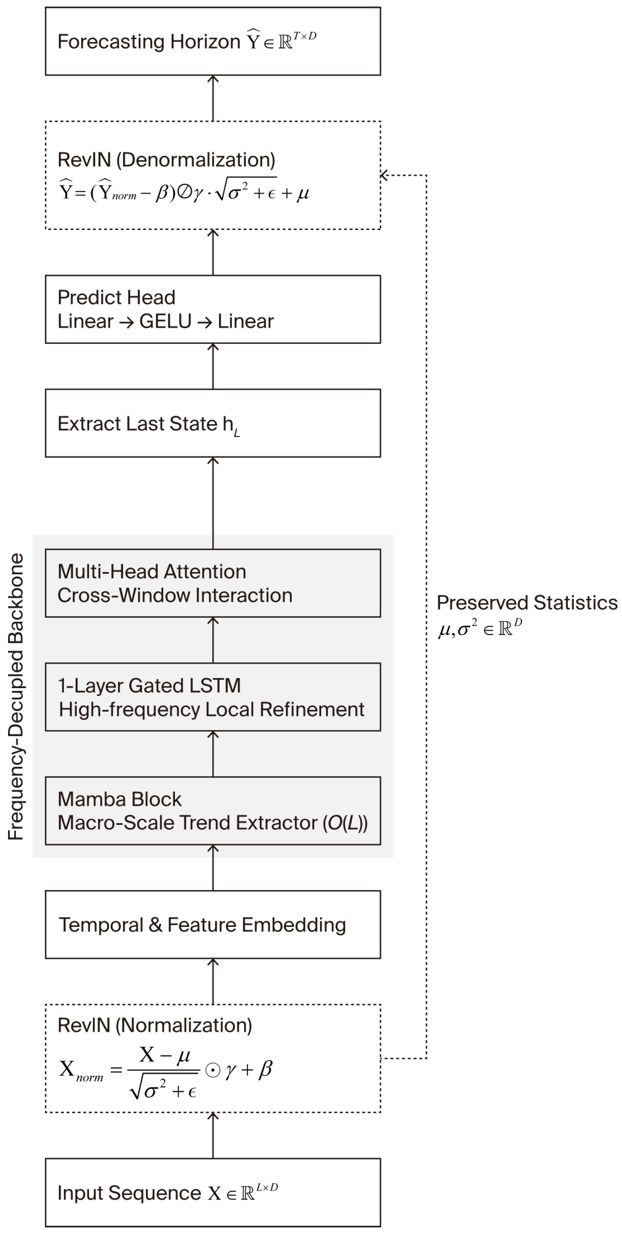
Figure 1 illustrates the overarching topology of the proposed Mamba-LSTM-Attention (MLA) framework, which is fundamentally structured as a progressive pipeline to address non-stationary distribution shifts and cross-horizon forecasting degradation. The architecture initiates with a de-stationarization phase, where a Reversible Instance Normalization (RevIN) module is applied to the historical multivariate load sequence $X\in {\mathbb{R}}^{L\times D}$. This module extracts and preserves the temporal mean $\mu$ and variance ${\sigma }^2$, thereby transforming the raw input into a standardized space $X_{norm}$ to neutralize statistical drift. Following this distribution alignment, the standardized sequence is projected into a high-dimensional space and processed by a frequency-decoupled temporal backbone. Within this hierarchical structure, a Selective State Space Model (Mamba) functions as the foundational macro-scale trend extractor, encoding expansive long-range dependencies with a linear computational complexity. To complement this global encoding, a single-layer gated LSTM is subsequently deployed to extract immediate non-linear dynamics and refine high-frequency local residuals. A Multi-Head Attention mechanism then dynamically re-weights these refined features to capture critical cross-window correlations. Consequently, to prevent the accumulation of high-frequency autoregressive errors across extended horizons, the architecture imposes an information bottleneck by extracting only the final hidden state $h_L$. A multi-layer perceptron maps this bottleneck state directly to the normalized future trajectory ${\widehat{Y}}_{norm}\in {\mathbb{R}}^{T\times D}$. In the final stage, a symmetric RevIN denormalization is executed, reinjecting the preserved statistical parameters $(\mu ,{\sigma }^2)$ to restore the precise physical scale and magnitude of the ultimate forecasting target $\widehat{Y}$.

3.2. Reversible Instance Normalization (RevIN) for Distribution Shift

Real-world electrical load sequences frequently exhibit non-stationary distribution shifts driven by environmental and socioeconomic anomalies. To mitigate the resultant statistical drift, the MLA architecture integrates a Reversible Instance Normalization (RevIN) module prior to representation learning. Given an input sequence instance $X\in {\mathbb{R}}^{L\times D}$, the module computes the temporal mean $\mu \in {\mathbb{R}}^D$ and variance ${\sigma }^2\in {\mathbb{R}}^D$ across the look-back window $L$. The instance is then standardized:

$$X_{norm}={\displaystyle \frac{X-\mu }{\sqrt{{\sigma }^2+ϵ}}}\odot \gamma +\beta$$

(1)

where $ϵ$ is a numerically stable constant, and $\gamma ,\beta \in {\mathbb{R}}^D$ denote learnable affine parameters designed to retain dimension-specific variance properties. Following the extraction of temporal dynamics and projection into the forecasting horizon $T$, a symmetrical denormalization operation is executed on the intermediate prediction ${\widehat{Y}}_{norm}\in {\mathbb{R}}^{T\times D}$:

$$\widehat{Y}=({\widehat{Y}}_{norm}-\beta )\oslash \gamma \cdot \sqrt{{\sigma }^2+ϵ}+\mu$$

(2)

This inverse transformation restores the original physical scale and non-stationary magnitude of the target variables, ensuring stable gradient propagation and limiting the error accumulation prevalent in standard deep learning architectures under anomalous grid demands.

3.3. Mamba State Space Model

To overcome the quadratic computational overhead ($O\left(L^2\right)$) of standard Transformer architectures, the MLA framework employs the Selective State Space Model (Mamba) to encode expansive long-range dependencies. The Mamba module parameterizes a continuous-time signal x(t) to a response y(t) via a latent state h(t), governed by linear ordinary differential equations (ODEs). To process discrete electrical load tokens, a Zero-Order Hold (ZOH) [15,16] discretization is applied. Modulated by a timescale parameter Δ, the continuous evolution matrices $A$ and $B$ are transformed into their discrete counterparts A and B:

$$\overline{A}=\mathit{exp}(\Delta A)$$

(3)

$$\overline{B}=(\Delta A{)}^{-1}(\mathit{exp}(\Delta A)-I)\cdot \Delta B$$

(4)

Consequently, the continuous ODEs are reformulated into an autoregressive discrete recurrence:

$$h_t=\overline{A}{h}_{t-1}+\overline{B}{x}_t$$

(5)

$$y_t=C{h}_t$$

(6)

By integrating hardware-aware parallel scans, this discrete recurrence achieves an empirical global receptive field with $O\left(L\right)$ linear time complexity. This module captures macroscopic temporal dependencies. Through its selective state mechanism, it systematically isolates essential long-term periodic trends and reduces uninformative stochastic noise prior to local refinement.

3.4. LSTM Unit

While the Mamba encoder efficiently establishes a macroscopic contextual foundation, it inherently smooths over transient fluctuations critical for precise load forecasting. To recapture these immediate non-linear dynamics, the MLA architecture cascades the Mamba output into a single-layer gated Long Short-Term Memory (LSTM) network. The LSTM unit is deployed to target localized fluctuations. It regulates the localized information flow through a tightly coupled gating mechanism, circumventing the mandate for long-range retention already fulfilled by the preceding state space module. At each discrete time step $t$, the input sequence is processed via an input gate $i_t$, a forget gate $f_t$, and an output gate $o_t$. The temporal evolution of the cell state $C_t$ and the hidden state $h_t$ is mathematically formalized as follows:

$$\begin{array}{ll}{i}_t& =\sigma (W_{xi}{x}_t+W_{hi}{h}_{t-1}+b_i)\\ f_t& =\sigma (W_{xf}{x}_t+W_{hf}{h}_{t-1}+b_f)\\ g_t& =tanh(W_{xg}{x}_t+W_{hg}{h}_{t-1}+b_g)\\ o_t& =\sigma (W_{xo}{x}_t+W_{ho}{h}_{t-1}+b_o)\\ c_t& =f_t\odot c_{t-1}+i_t\odot g_t\\ h_t& =o_t\odot tanh(c_t)\end{array}$$

(7)

The frequency-domain decoupling is enforced by restricting this operation to a single parametric layer. Because the preceding Mamba module already encodes macroscopic long-range dependencies, deploying a multi-layer LSTM would introduce overlapping temporal receptive fields and redundant parameterization. By utilizing exactly one layer, the recurrent capacity is deliberately limited, forcing the LSTM unit to focus exclusively on immediate high-frequency residuals. This minimal configuration establishes a complementary feature extraction pipeline while preserving the linear-time computational efficiency of the framework.

3.5. Multi-Head Attention Mechanism

To dynamically align and re-weight the refined multi-scale features, the LSTM representations are subsequently projected into a Multi-Head Attention mechanism. This module computes cross-window correlations by mapping the temporal sequence into distinct $\mathrm{Q}\mathrm{u}\mathrm{e}\mathrm{r}\mathrm{y}\left(Q\right)$, $\mathrm{K}\mathrm{e}\mathrm{y}\left(K\right)$, and $\mathrm{V}\mathrm{a}\mathrm{l}\mathrm{u}\mathrm{e}\left(V\right)$ matrices across multiple representation subspaces [9]. The attention weights are calculated via scaled dot-product operations, formulated as

$$Attention(Q,K,V)=softmax\left({\displaystyle \frac{Q{K}^T}{\sqrt{d_k}}}\right)V$$

(8)

where $d_k$ represents the dimensionality of each attention head. This parallel re-weighting emphasizes critical transient shifts within the historical look-back window. However, to translate this sequence-level representation into a multi-step future trajectory without incurring cumulative autoregressive errors, the architecture implements a structural information bottleneck. Rather than mapping the entire temporal sequence, the network isolates the final aggregated hidden state $h_L$ from the attention output matrix. The preceding Multi-Head Attention module computes cross-channel and cross-window correlations prior to this bottleneck. Consequently, the terminal state $h_L$ functions as a fully contextualized vector encompassing the synergistic multivariate interactions, preserving critical cross-channel fidelity. A subsequent multi-layer perceptron utilizes this isolated bottleneck vector to directly decode the standardized multi-step forecasting horizon $Y_{norm}$, thereby structurally bounding the error propagation commonly observed in prolonged sequential decoding.

3.6. Architecture Integration and Optimization Strategy

The MLA framework is designed as an end-to-end differentiable architecture mapping multivariate historical sequences $X$ to future trajectories $\widehat{Y}$. The structural topology follows the progressive feature evolution pipeline: the input sequence is initially standardized via the RevIN module to neutralize distribution shifts, followed by dimensional alignment through an embedding layer. The representation is subsequently processed by the cascaded Mamba-LSTM-Attention backbone. To prevent error accumulation across extended forecasting horizons, the architecture imposes an information bottleneck by extracting only the final aggregated hidden state from the attention mechanism, which is then projected via a multi-layer perceptron and denormalized by RevIN to yield the final prediction.

To ensure optimal training dynamics and maximize parameter efficiency, the hyperparameter space was systematically tuned using Tree-structured Parzen Estimator (TPE) Bayesian optimization [5] rather than conventional grid search. Based on the TPE convergence, the hidden dimension is established at 128, and a consistent sequence look-back window of $L=96$ is utilized to evaluate forecasting horizons $T\in \{96,192,336,720\}$. To mitigate overfitting risks inherent in deep hybrid structures, Dropout regularization $p=0.3$ is uniformly applied across residual connections and attention weights.

The training process employs a customized Huber Loss objective [44] to penalize prediction outliers. The mathematical formulation is defined as:

$$L_{\delta }(y,\widehat{y})=\left\{\begin{array}{ll}{\displaystyle \frac{1}{2}}(y-\widehat{y}{)}^2& for|y-\widehat{y}|\le \delta \\ \delta |y-\widehat{y}|-{\displaystyle \frac{1}{2}}{\delta }^2& otherwise\end{array}\right.$$

(9)

where $y$ represents the ground truth, $\widehat{y}$ denotes the predicted value, and the transition threshold is set to $\delta =1.0$. This piecewise function diminishes gradient sensitivity to anomalous load spikes. The network parameters are updated utilizing the AdamW optimizer with a decoupled weight decay of $3.74\times 10^{-6}$ and a learning rate of $2.84\times 10^{-4}$, to ensure robust generalization on unseen grid data.

3.7. Synergistic Mechanism and Theoretical Justification

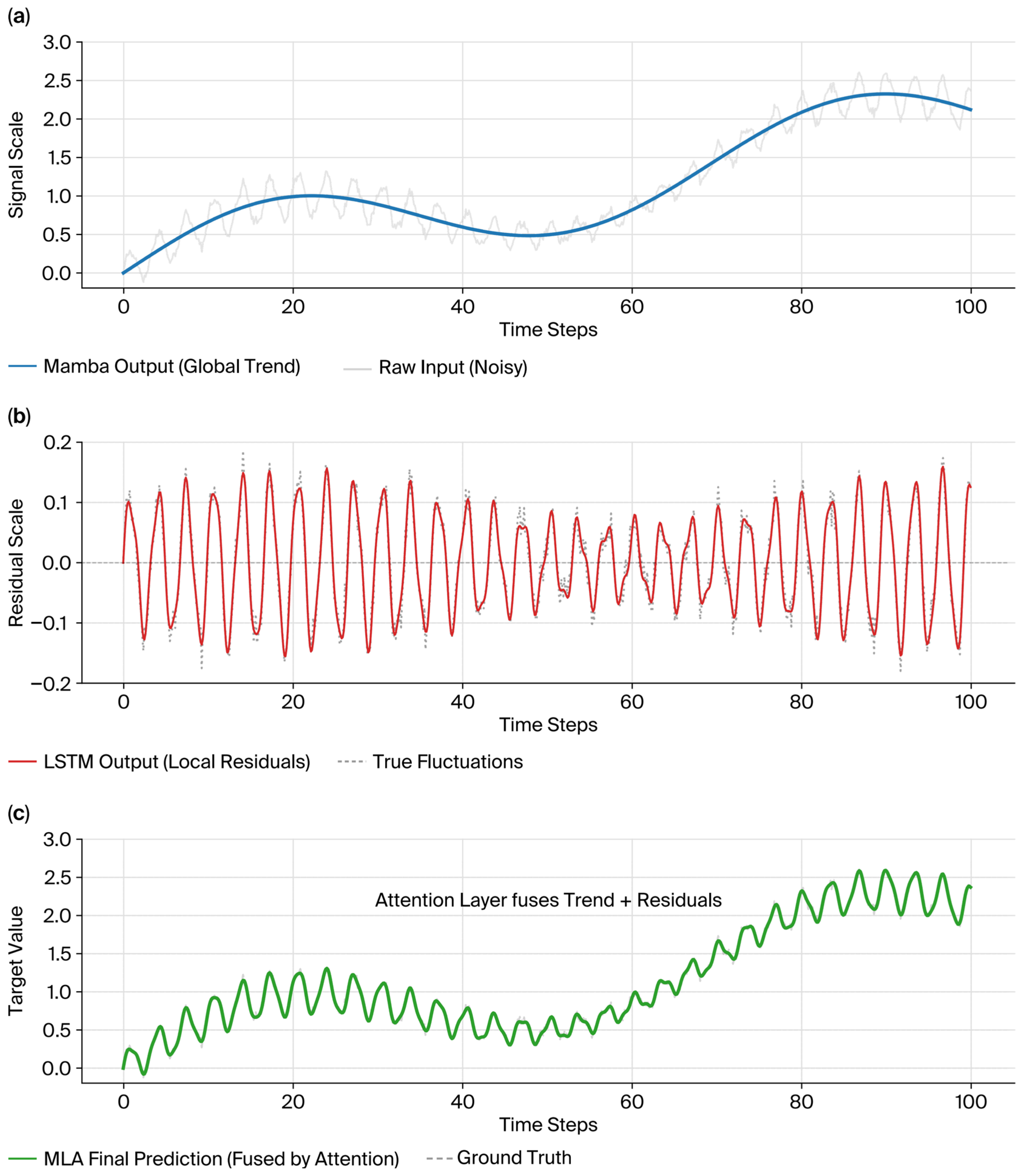
The empirical efficacy of the MLA architecture is fundamentally grounded in its hierarchical “Global-to-Local” feature evolution pipeline. As visualized in Figure 2, this progressive extraction process can be functionally interpreted through a frequency-domain perspective. Specifically, the Mamba module extracts the dominant macroscopic trends over extended horizons. Building upon this macro-scale foundation, the single-layer gated LSTM models the localized non-linear transient residuals that the selective state space mechanism inherently smooths over. Following this decoupling, the Multi-Head Attention mechanism applies adaptive re-weighting to dynamically fuse these multi-scale signals. Notably, rather than employing a traditional iterative autoregressive decoder, the MLA framework consolidates these features through a single-point linear projection. This structural information bottleneck inevitably sacrifices a degree of marginal short-term precision to enhance cross-horizon stability. By extracting only the terminal hidden state, this bottleneck restricts the propagation of microscopic fluctuations. It suppresses the exponential error accumulation typically induced by prolonged sequential decoding, thereby prioritizing long-term structural robustness over immediate point-wise accuracy.

4. Experimental Results and Analysis

4.1. Benchmark Datasets and Data Preprocessing

To evaluate the proposed MLA architecture, empirical experiments were conducted across four standard multivariate benchmark datasets: ETTh1, ETTh2, ETTm1, and ETTm2. These datasets record dynamic electrical load metrics at varying temporal granularities of one hour and fifteen minutes, exhibiting diverse degrees of periodicity and non-stationary structural mutations. Although the primary target variable in the ETT benchmarks is transformer oil temperature, it serves as a highly reliable proxy for macroscopic grid load dynamics. As established by the original architects of the ETT dataset [9], transformer temperature is a direct reflection of underlying grid dispatching stress and equipment health. This empirical substitution is fundamentally supported by the thermodynamic physics of power transformers, where internal temperature fluctuations are predominantly driven by copper losses that are directly proportional to the square of the active electrical load current [45]. Consequently, the non-stationary structural mutations observed in the ETTh2 and ETTm2 sequences mirror the volatility of actual grid dispatching demands, making these datasets a robust testbed for evaluating architectural robustness against real-world load anomalies. To ensure a fair empirical comparison with established baselines, a standard chronological dataset splitting protocol is used to evaluate the proposed framework. The dataset sequences are partitioned into training, validation, and testing sets in a 7:1:2 ratio. The validation set functions exclusively to tune hyperparameters and select the optimal model checkpoint, which prevents temporal data leakage. The model’s predictive performance is quantified using Mean Squared Error (MSE) as the primary optimization objective to penalize extreme prediction outliers, complemented by Mean Absolute Error (MAE) to measure the average physical magnitude of the forecasting deviation. Furthermore, to quantify the framework’s structural robustness against horizon extension, the Coefficient of Variation across Horizons $\left(C{V}_H\right)$ is introduced as a core stability metric, formulated as

$$C{V}_H={\displaystyle \frac{{\sigma }_{MSE}}{{\mu }_{MSE}}}\times 100\%$$

(10)

where ${\sigma }_{MSE}$ and ${\mu }_{MSE}$ represent the standard deviation and the mean of the corresponding MSE values across the four target horizons $(T\in \{96,192,336,720\left\}\right)$, respectively. A lower $C{V}_H$ indicates competitive cross-step forecasting consistency, which constitutes a critical prerequisite for reliable long-term grid dispatching. The absolute deviation at discrete horizons is evaluated using standard metrics. However, these discrete values do not provide a comprehensive picture of the temporal degradation trajectory. The Coefficient of Variation across Horizons ($C{V}_H$) is therefore introduced in order to evaluate the consistency of forecasts made across steps. $C{V}_H$ is defined as a conditional evaluation metric. A relative stability is only considered valuable when the absolute MSE is maintained within a threshold that is operationally viable. The results of models with large absolute errors are disregarded when there is a conflict between relative stability and absolute accuracy, because they produce unusable predictions despite their low variance. The statistical descriptions of the benchmark datasets are summarized in

Table 2. Summary and statistical descriptions of the benchmark datasets. Source: China Southern Power Grid; National Energy Administration; Zhou et al. [9].

Dataset	Domain	Time Granularity	Dimension (D)	Target Variable	Sequence Characteristics Analysis
ETTh1	Electricity	1 h	7	Oil Temperature	Moderate periodicity; serves as the baseline reference point.
ETTh2	Electricity	1 h	7	Oil Temperature	Contains significant structural mutations.
ETTm1	Electricity	15 min	7	Oil Temperature	High-frequency sampling; complex short-term fluctuations.
ETTm2	Electricity	15 min	7	Oil Temperature	High-frequency sampling; complex short-term non-linear fluctuations.
Electricity	Electricity	1 h	321	Electricity Consumption	True consumer-driven non-stationarity; directly represents real-world smart grid load dynamics.

.

4.2. Experimental Setup and Hyperparameters

The empirical evaluation compares the proposed MLA framework against baseline models representing distinct architectural paradigms. All baseline architectures were reproduced locally to ensure a strictly equivalent comparison. Specifically, the implementations for Informer, Autoformer, PatchTST, and iTransformer were sourced directly from the Tsinghua University Time-Series-Library. The S-Mamba architecture was sourced from the official reference repository provided by Wang et al. [46]. This targeted selection covers the primary evolutionary branches of forecasting networks. It provides a structurally diverse context to validate the proposed framework, negating the necessity of compiling an exhaustive list of minor architectural variants.

All comparative experiments were run on a unified hardware platform equipped with an NVIDIA RTX 4090 GPU. To ensure empirical reproducibility, the global random seed was fixed at 42 across all execution environments. The hyperparameter configuration aligns with the optimal parameter space identified through the Tree-structured Parzen Estimator (TPE) Bayesian optimization [5] detailed in Section 3.6. Specifically, the historical look-back window was fixed at 96 and projected the raw inputs into a 128-dimensional continuous space via a linear embedding layer. Within the frequency-decoupled backbone, the Mamba state dimension operates at 64. The high-frequency residual extraction utilizes a single-layer gated LSTM, while the cross-window interaction employs 8 parallel attention heads. To mitigate overfitting, a consistent Dropout rate of 0.3 functions across the residual connections, the attention mechanism, and the fully connected prediction head. The network weights were optimized using the AdamW optimizer with a learning rate of 0.000284, a decoupled weight decay of 3.74 × 10⁻⁶, and a batch size of 64. The training configuration established a fixed computational budget of 15 epochs. To ensure optimal model selection without premature termination, the validation loss was continuously monitored at the end of each epoch. The system systematically saved the model checkpoint whenever the validation error reached a new minimum. Upon completing the entire 15-epoch budget, the optimal network weights from the saved checkpoint were loaded to execute the final testing phase. This configuration ensures stable convergence under the Huber Loss objective, which operates with a standard threshold of [44].

Table 3. Detailed hyperparameter configurations for the proposed MLA model. Source: (Author’s own work).

No.	Configuration	Value	Description (Corresponding Code Elements)
1	Historical look-back window	96	Length of historical observation window (seq_len) and forecasting horizon (pred_len).
2	Prediction horizon	{96, 192, 336, 720}	Length of historical observation window (seq_len) and forecasting horizon (pred_len).
3	Internal Feature Embedding Dim	128	Dimension of internal feature embedding.
4	Mamba State Dim	64	State space dimension of the SSM.
5	LSTM Layers	1	Number of stacked LSTM layers.
6	Dropout rate	0.3	Unified dropout rate applied across LSTM, Attention, and FC layers.
7	Learning Rate	2.84 × 10−4	Learning rate and L2 weight decay for the AdamW optimizer.
8	Weight Decay	3.74 × 10−6	Learning rate and L2 weight decay for the AdamW optimizer.
9	Attention Heads	8	Number of parallel attention heads for cross-window interaction.
10	Optimizer	AdamW	Optimization algorithm for network weight updates.
11	Loss function	Huber Loss (δ = 1.0)	Objective function for robust error optimization.
12	Batch Size	64	Number of sequence samples processed in one training iteration.
13	Epoch Budget	15	Maximum limit of complete passes through the training dataset.

summarizes the detailed parameters.

4.3. Experimental Results and Discussion

The quantitative evaluation against recent baselines reveals a trade-off between point-wise precision and cross-horizon stability (

Table 4. Forecasting performance of the proposed MLA framework and baseline models. All baseline architectures were reproduced locally. The metrics are derived from independent experiments conducted under identical hardware configurations and standard sequential dataset splitting protocols (7:1:2).

Dataset	Model	T = 96 MSE/MAE/RMSE	T = 192 MSE/MAE/RMSE	T = 336 MSE/MAE/RMSE	T = 720 MSE/MAE/RMSE	$\mathit{C}{\mathit{V}}_{\mathit{H}}$
ETTh1	Autoformer	0.449/0.459/0.670	0.500/0.482/0.707	0.521/0.496/0.722	0.542/0.524/0.736	7.93%
	PatchTST	0.419/0.424/0.647	0.469/0.454/0.685	0.501/0.466/0.708	0.500/0.488/0.707	8.15%
	S-Mamba	0.386/0.405/0.621	0.443/0.437/0.666	0.499/0.468/0.706	0.502/0.499/0.709	11.99%
	iTransformer	0.386/0.405/0.621	0.441/0.436/0.664	0.487/0.458/0.698	0.503/0.491/0.709	11.57%
	MLA	0.566/0.538/0.752	0.601/0.564/0.775	0.640/0.589/0.800	0.764/0.660/0.874	13.43%
ETTh2	Autoformer	0.346/0.388/0.588	0.456/0.452/0.675	0.482/0.486/0.694	0.515/0.539/0.718	16.29%
	PatchTST	0.342/0.384/0.585	0.388/0.400/0.623	0.426/0.433/0.653	0.431/0.446/0.657	10.40%
	S-Mamba	0.296/0.348/0.544	0.376/0.396/0.613	0.424/0.431/0.651	0.426/0.444/0.653	16.00%
	iTransformer	0.297/0.349/0.545	0.380/0.400/0.616	0.428/0.432/0.654	0.427/0.445/0.653	16.07%
	MLA	0.210/0.317/0.458	0.237/0.343/0.487	0.253/0.353/0.503	0.304/0.387/0.551	15.75%
ETTm1	Autoformer	0.505/0.475/0.711	0.553/0.496/0.744	0.621/0.537/0.788	0.671/0.561/0.819	12.47%
	PatchTST	0.329/0.367/0.574	0.367/0.385/0.606	0.399/0.410/0.632	0.454/0.439/0.674	13.66%
	S-Mamba	0.333/0.368/0.577	0.376/0.390/0.613	0.408/0.413/0.639	0.475/0.448/0.689	15.03%
	iTransformer	0.334/0.368/0.578	0.377/0.391/0.614	0.426/0.420/0.653	0.491/0.459/0.701	16.57%
	MLA	0.474/0.471/0.688	0.533/0.498/0.730	0.591/0.537/0.769	0.637/0.563/0.798	12.66%
ETTm2	Autoformer	0.255/0.339/0.505	0.348/0.403/0.590	0.509/0.472/0.713	0.433/0.432/0.658	28.34%
	PatchTST	0.175/0.259/0.418	0.241/0.302/0.491	0.305/0.343/0.552	0.402/0.400/0.634	34.16%
	S-Mamba	0.179/0.263/0.423	0.250/0.309/0.500	0.312/0.349/0.558	0.411/0.406/0.642	34.44%
	iTransformer	0.180/0.264	0.250/0.309	0.311/0.348	0.412/0.407/0.642	34.12%
	MLA	0.128/0.242/0.358	0.160/0.272/0.400	0.204/0.305/0.452	0.260/0.349/0.510	30.44%
Electricity	Autoformer	0.201/0.317/0.448	0.222/0.334/0.471	0.231/0.338/0.481	0.254/0.361/0.504	9.67%
	PatchTST	0.181/0.270/0.425	0.188/0.274/0.434	0.204/0.293/0.452	0.246/0.324/0.496	14.23%
	S-Mamba	0.139/0.235/0.373	0.159/0.255/0.399	0.176/0.272/0.420	0.204/0.298/0.452	16.24%
	iTransformer	0.148/0.240/0.385	0.162/0.253/0.402	0.178/0.269/0.422	0.225/0.317/0.474	18.79%
	MLA	0.187/0.291/0.432	0.203/0.304/0.451	0.212/0.313/0.460	0.230/0.326/0.480	8.63%

). The MLA architecture yields lower forecasting errors in non-stationary environments characterized by distribution shifts. On the ETTh2 dataset, the model establishes an MSE of 0.210 at the T = 96 horizon. This result outperforms channel-independent models like PatchTST (0.342) and multivariate architectures, including iTransformer (0.297) and S-Mamba (0.296). The framework replicates this performance on the ETTm2 dataset, achieving a lower absolute MSE (0.128) than the iTransformer baseline (0.180).

To evaluate the efficacy for real-world smart grid operations, the empirical analysis extends to the Electricity dataset. This sequence exhibits consumer-driven non-stationarity across 321 interconnected nodes. Multivariate models like iTransformer and S-Mamba prioritize short-term precision on this dataset, achieving initial MSEs of 0.148 and 0.139 at T = 96. However, they exhibit error compounding across extended horizons, resulting in Coefficient of Variation across Horizons ($C{V}_H$) metrics of 18.79% and 16.24%. In contrast, the MLA framework restricts autoregressive error propagation. It records a structural degradation rate of 8.63% ($C{V}_H$) on the 321-dimensional network. By imposing a terminal information bottleneck, the architecture trades marginal short-term amplitude tracking for long-range forecasting consistency.

Conversely, ETTh1 and ETTm1 sequences exhibit stationary properties with high-frequency periodic patterns. The MLA framework yields lower absolute accuracy on these benchmarks. This performance divergence originates from the interaction between sequence statistical characteristics and architectural constraints. The terminal information bottleneck smooths fine-grained periodic details to prioritize long-range stability. While this structural bottleneck prevents error compounding during structural shifts, it limits the capacity to capture peak amplitudes required to minimize errors on periodic sequences. Furthermore, while models like PatchTST achieve lower relative $C{V}_H$ on these stationary datasets, they coincide with a higher absolute error baseline. An inaccurate baseline prediction trajectory holds limited utility for practical dispatching operations. The MLA framework operates as a specialized architecture for industrial smart grids. It prioritizes stable forecasting trajectories under volatility over marginal accuracy gains in periodic scenarios.

4.4. Ablation Study

The ablation study evaluates the individual contribution of each architectural component on the non-stationary ETTh2 dataset and the highly stationary ETTh1 dataset.

Table 5. Results of the ablation study on the ETTh2 and ETTh1 dataset. Source: (Author’s own work).

Model Variant	Component Removed	ETTh2			ETTh1
		MSE	MAE	ΔMSE (vs. Base)	MSE	MAE	ΔMSE (vs. Base)
MLA(Proposed)	None	0.210	0.317	—	0.566	0.538	—
MLA	RevIN	0.431	0.495	+105.24%	0.716	0.616	+26.50%
LSTM-Attention	Mamba	0.218	0.321	+3.81%	0.571	0.533	+0.88%
Mamba-LSTM	Attention	0.223	0.329	+6.19%	0.633	0.552	+11.84%
Mamba-Attention	LSTM	0.227	0.325	+8.10%	0.582	0.546	+2.83%

details the divergent performance trajectories across these two environments.

On the ETTh2 dataset, the complete MLA framework achieves an optimal MSE of 0.210. Removing the RevIN module increases the MSE to 0.431. This result confirms that symmetric distribution alignment maintains gradient stability under structural mutations. Metrics indicate a complementary relationship within the temporal backbone. Bypassing the multi-head attention mechanism (Mamba-LSTM variant) disrupts cross-window feature fusion and increases the MSE to 0.223. Substituting the Mamba encoder (LSTM-Attention variant) raises the MSE to 0.218. Eliminating the LSTM unit (Mamba-Attention variant) yields an MSE of 0.227. These metrics show that the localized modeling of the single-layer LSTM is equally important as the macroscopic trend extraction of the Mamba module in non-stationary environments.

Conversely, the ablation results on the stationary ETTh1 dataset demonstrate a minimal performance impact when removing structural components. Bypassing the Mamba module (LSTM-Attention variant) increases the MSE by only 0.88% (from 0.566 to 0.571). Eliminating the LSTM unit (Mamba-Attention variant) raises the MSE by 2.83% (from 0.566 to 0.582). In contrast, removing these exact components on the volatile ETTh2 dataset increases the MSE by 3.81% and 8.10%, respectively.

This empirical divergence validates the architectural design. The cascaded Mamba-LSTM topology and the RevIN module function as anti-drift mechanisms engineered to neutralize non-stationary anomalies. In highly regular environments lacking structural mutations, the advanced anti-drift capacity of these components is not fully engaged. The complete architecture yields performance comparable to its simplified variants. These results validate the precision–stability trade-off. They demonstrate that the MLA framework is fundamentally optimized to ensure forecasting robustness under high grid volatility.

4.5. Qualitative Evaluation and Visualization

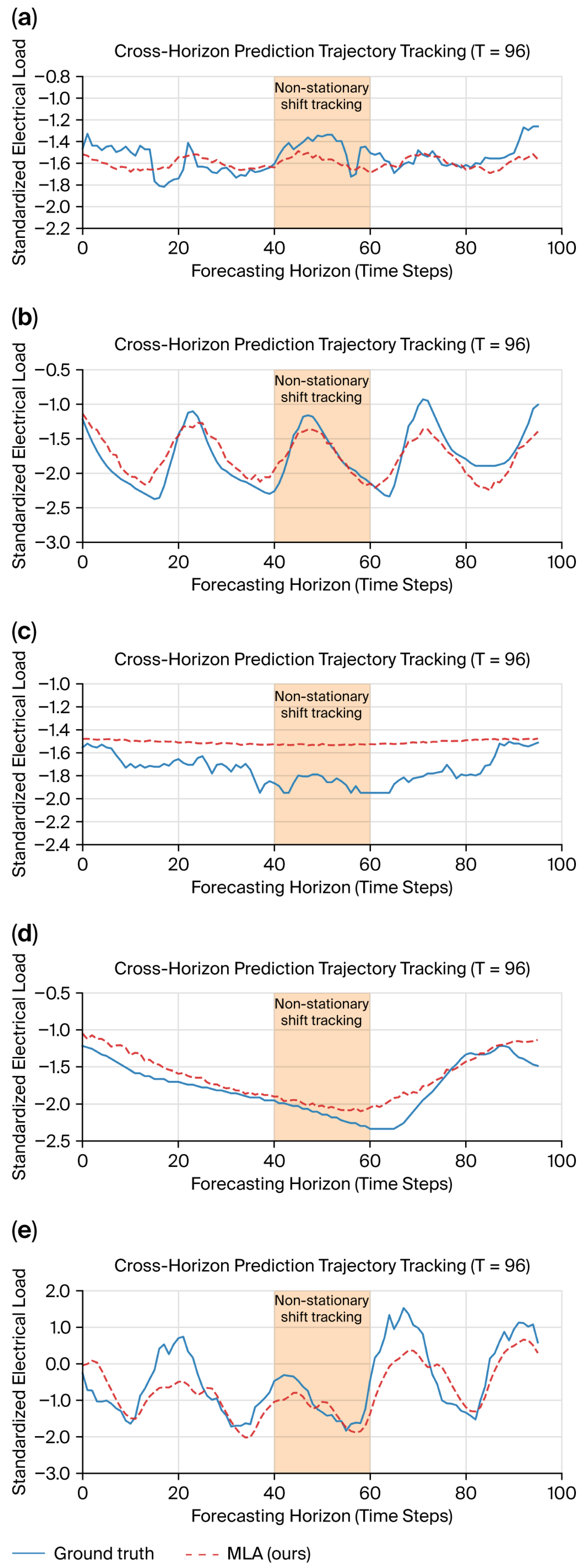
Forecasting trajectories across the five evaluated datasets at the T = 96 horizon provides intuitive validation of the precision–stability trade-off (Figure 3). These visualizations, ordered (a–e) corresponding to ETTh1, ETTh2, ETTm1, ETTm2, and Electricity, exhibit varying adaptability in the frequency-decoupled framework.

Non-stationary sequences exhibit structural mutations captured by the architecture. On the ETTh2 dataset (Figure 3b), standardized electrical load undergoes distribution shifts within the highlighted region (time steps 40–60). The model maintains phase alignment and tracks amplitude changes during this period. The ETTm2 sequence similarly shows tracking of the overarching U-shaped recovery (Figure 3d). Furthermore, primary structural fluctuations are tracked on the dynamic Electricity dataset (Figure 3e). This tracking behavior confirms the capacity of the RevIN and LSTM modules to model non-linear residuals during distribution shifts.

Conversely, ETTh1 and ETTm1 trajectories illustrate the operational effect of the information bottleneck, prioritizing macroscopic trends over high-frequency variance. On the periodic ETTh1 sequence (Figure 3a), consistent phase alignment is achieved while applying conservative amplitude smoothing on marginal high-frequency spikes. Microscopic fluctuations are smoothed under the 15 min sampling resolution of ETTm1 (Figure 3c) to output a stable macroscopic baseline. This structural design restricts autoregressive error accumulation across extended horizons. The cross-dataset visual analysis proves the architecture balances high-frequency noise suppression with transient shift tracking for industrial grid operations.

4.6. Computational Efficiency Analysis

The computational efficiency analysis derives directly from the aforementioned local reproduction process. All baseline models and the proposed MLA framework were evaluated under identical hardware constraints. Computational benchmarks quantify the hardware footprint of the evaluated architectures (

Table 6. Computational efficiency comparison of different architectures. Evaluated on a single NVIDIA RTX 4090 GPU (Look-back window 96, Batch Size 64).

Model	Architecture Type	Training Time (s/Epoch)	Peak Memory (MB)
Autoformer	Transformer-based	4.31	233.28
PatchTST	Transformer-based	3.49	1602.87
S-Mamba	State-Space Model	2.69	147.11
iTransformer	Transformer-based	6.16	161.91
MLA (Ours)	Hybrid (SSM + LSTM)	1.69	175.99

). The empirical evaluation is executed on a single NVIDIA RTX 4090 GPU under identical configurations (look-back window 96, batch size 64). Standard Transformer architectures incur substantial operational overhead. Autoformer requires 4.31 s per epoch. PatchTST reduces this training duration to 3.49 s but consumes 1602.87 MB of peak memory due to its channel-independent patching mechanism. The iTransformer addresses this memory demand. Employing dimension inversion, it limits peak memory allocation to 161.91 MB, though it requires a longer sequential processing time of 6.17 s per epoch.

State-space architectures provide a faster operational alternative. The pure state-space baseline, S-Mamba, requires 2.69 s per epoch and 147.11 MB of peak memory. The proposed MLA framework records an execution time of 1.69 s per epoch with a peak memory allocation of 175.99 MB. The streamlined computational graph of the MLA framework executes faster than the bidirectional sweep mechanism of S-Mamba. Cascading the single-layer LSTM after the Mamba backbone introduces a 28.88 MB memory overhead compared to S-Mamba, but it avoids the memory saturation typical of standard attention networks.

These operational metrics confirm a trade-off among computational efficiency, point-wise precision, and cross-horizon stability. Standard attention mechanisms prioritize short-term precision on stationary sequences at the expense of hardware efficiency. The MLA architecture confines the quadratic attention computation to the final bottleneck stage. This configuration intentionally limits the capacity to capture high-frequency periodic patterns, yielding higher point-wise errors on stationary datasets such as ETTh1. However, this structural constraint bounds exponential error compounding and ensures stable forecasting trajectories under non-stationary shifts. The MLA framework serves as a resource-efficient baseline for volatile industrial grid deployments.

4.7. Hyperparameter Sensitivity Analysis

The hyperparameter sensitivity analysis evaluates the structural robustness of the MLA architecture during the TPE optimization phase (

Table 7. Hyperparameter sensitivity analysis derived from the empirical TPE optimization trials.

Hyperparameter	Range Tested	Optimal Value	Sensitivity	Impact on MSE
Hidden Layers (LSTM)	{1, 2, 3}	1	High	Sharp degradation from 8.59 (1 layer) to 9.68 (3 layers)
Learning Rate	{1.1 × 10−5, 8.5 × 10−4}	2.84 × 10−4	High	Suboptimal convergence at boundaries (e.g., MSE 9.13 at 1.1 × 10−5)
Hidden Dimension	{128, 256, 512}	128	Low	High stability across scales (MSE 8.59 at 128 vs. 8.66 at 512)
Dropout Rate	{0.1, 0.2, 0.3, 0.4}	0.3	Low	Marginal MSE variance (8.59 to 8.75) across the full range

). This evaluation monitors the impact of the LSTM layer count, learning rate, hidden dimension, and dropout rate on the validation MSE.

The architecture exhibits structural sensitivity to the number of recurrent layers. Configurations utilizing a single LSTM layer yield an optimal MSE of 8.59. Increasing the recurrent depth to three layers increases the MSE to 9.68. This empirical penalty validates the architectural constraint limiting the LSTM to a single-layer transient extractor. The model similarly demonstrates high sensitivity to the learning rate. The optimization trajectory converges optimally at 2.84 × 10⁻⁴. Deviating to the search boundaries—such as dropping to 1.1 × 10⁻⁵ or exceeding 8.5 × 10⁻⁴—disrupts gradient stability and increases the MSE beyond 8.98.

Conversely, the framework demonstrates robust stability regarding the hidden dimension and dropout rate. The model maintains stable MSE values (8.59 at 128 and 8.66 at 512) across different hidden dimensions. It also remains stable across dropout rates, showing marginal variance (MSE ranging from 8.59 to 8.75) when the dropout shifts between 0.1 and 0.4. This verified resilience to embedding dimensions, and regularization confirms the core hypothesis. The predictive precision originates from the frequency-decoupled structural design, not from high-dimensional parameter memorization.

5. Conclusions and Future Work

This study addressed the challenge of modeling non-stationary distribution shifts and mitigating long-range error accumulation in multivariate time series forecasting for smart grids. We proposed the Mamba-LSTM-Attention (MLA) framework, engineered around a progressive frequency-domain feature evolution pipeline. Integrating the RevIN module neutralizes statistical drift. Furthermore, the architectural decoupling between the linear-time Mamba module and the single-layer gated LSTM extracts both macroscopic trends and transient residuals.

Evaluations across benchmark datasets revealed a precision–stability trade-off governed by the model’s terminal information bottleneck. In non-stationary environments, the MLA architecture demonstrates predictive stability. The model establishes MSEs of 0.210 and 0.128 on the ETTh2 and ETTm2 datasets, respectively. Conversely, this structural bottleneck prioritizes long-range stability at the expense of capturing fine-grained periodic components. The framework consequently yields lower absolute accuracy on stationary datasets such as ETTh1 and ETTm1.

Nevertheless, this architectural constraint bounds error accumulation during load anomalies. The MLA framework provides a computation-efficient baseline optimized for industrial grid dispatching under structural mutations. To resolve the adaptability constraints in periodic scenarios, future research may explore adaptive Sequence-to-Sequence (Seq2Seq) decoding pathways and learnable parallel feature gating. These mechanisms aim to recover periodic inductive biases while maintaining non-stationary robustness.

References

1. Massaoudi, M.; Abu-Rub, H.; Refaat, S.S.; Chihi, I.; Oueslati, F.S. Deep learning in smart grid technology: A review of recent advancements and future prospects. IEEE Access 2021, 9, 54558–54578. [Google Scholar] [CrossRef]
2. Liu, Y.; Tian, Y.; Zhao, Y.; Yu, H.; Xie, L.; Wang, Y.; Ye, Q.; Jiao, J.; Liu, Y. Vmamba: Visual state space model. Adv. Neural Inf. Process. Syst. 2024, 37, 103031–103063. [Google Scholar]
3. Das, A.; Kong, W.; Leach, A.; Mathur, S.; Sen, R.; Yu, R. Long-term forecasting with Tide: Time-series dense encoder. arXiv 2023, arXiv:2304.08424. [Google Scholar]
4. Kim, T.; Kim, J.; Tae, Y.; Park, C.; Choi, J.-H.; Choo, J. Reversible instance normalization for accurate time-series forecasting against distribution shift. In Proceedings of the International Conference on Learning Representations, Virtual Event, 3–7 May 2021. [Google Scholar]
5. Bergstra, J.; Bardenet, R.; Bengio, Y.; Kégl, B. Algorithms for hyper-parameter optimization. Adv. Neural Inf. Process. Syst. 2011, 24, 2546–2554. [Google Scholar]
6. Lim, B.; Arık, S.Ö.; Loeff, N.; Pfister, T. Temporal fusion transformers for interpretable multi-horizon time series forecasting. Int. J. Forecast. 2021, 37, 1748–1764. [Google Scholar] [CrossRef]
7. Zhang, D.; Han, X.; Deng, C. Review on the research and practice of deep learning and reinforcement learning in smart grids. CSEE J. Power Energy Syst. 2018, 4, 362–370. [Google Scholar] [CrossRef]
8. Ibrahim, R.A.; Hebala, A. A Feature-Enhanced Approach to Dissolved Gas Analysis for Power Transformer Health Prediction Through Interpretable Ensemble Learning and Multi-Model Evaluation. Technologies 2025, 14, 6. [Google Scholar] [CrossRef]
9. Vaswani, A.; Shazeer, N.; Parmar, N.; Uszkoreit, J.; Jones, L.; Gomez, A.N.; Kaiser, Ł.; Polosukhin, I. Attention is all you need. arXiv 2017, arXiv:1706.03762. [Google Scholar]
10. Zhou, H.; Zhang, S.; Peng, J.; Zhang, S.; Li, J.; Xiong, H.; Zhang, W. Informer: Beyond efficient transformer for long sequence time-series forecasting. In Proceedings of the AAAI Conference on Artificial Intelligence, Palo Alto, CA, USA, 2–9 February 2021; pp. 11106–11115. [Google Scholar]
11. Lai, G.; Chang, W.-C.; Yang, Y.; Liu, H. Modeling long-and short-term temporal patterns with deep neural networks. In Proceedings of the 41st International ACM SIGIR Conference on Research & Development in Information Retrieval, Ann Arbor, MI, USA, 12 July 2018; pp. 95–104. [Google Scholar]
12. Lim, B.; Zohren, S. Time-series forecasting with deep learning: A survey. Philos. Trans. R. Soc. A 2021, 379, 20200209. [Google Scholar] [CrossRef]
13. Salinas, D.; Flunkert, V.; Gasthaus, J.; Januschowski, T. DeepAR: Probabilistic forecasting with autoregressive recurrent networks. Int. J. Forecast. 2020, 36, 1181–1191. [Google Scholar] [CrossRef]
14. Wu, H.; Xu, J.; Wang, J.; Long, M. Autoformer: Decomposition transformers with auto-correlation for long-term series forecasting. Adv. Neural Inf. Process. Syst. 2021, 34, 22419–22430. [Google Scholar]
15. Gu, A.; Goel, K.; Ré, C. Efficiently modeling long sequences with structured state spaces. arXiv 2021, arXiv:2111.00396. [Google Scholar]
16. Gu, A.; Dao, T. Mamba: Linear-time sequence modeling with selective state spaces. arXiv 2023, arXiv:2312.00752. [Google Scholar] [CrossRef]
17. Zhu, L.; Liao, B.; Zhang, Q.; Wang, X.; Liu, W.; Wang, X. Vision mamba: Efficient visual representation learning with bidirectional state space model. arXiv 2024, arXiv:2401.09417. [Google Scholar] [CrossRef]
18. Yang, Y.J.; Xing, Z.H.; Yu, L.Q.; Fu, H.Z.; Huang, C.W.; Zhu, L. Vivim: A Video Vision Mamba for Ultrasound Video Segmentation. IEEE Trans. Circ. Syst. Vid. 2025, 35, 10293–10304. [Google Scholar] [CrossRef]
19. Zhang, T.; Yuan, H.; Qi, L.; Zhang, J.; Zhou, Q.; Ji, S.; Yan, S.; Li, X. Point cloud mamba: Point cloud learning via state space model. In Proceedings of the AAAI Conference on Artificial Intelligence, Palo Alto, CA, USA, 25 February–4 March 2025; pp. 10121–10130. [Google Scholar]
20. Gu, A.; Goel, K.; Gupta, A.; Ré, C. On the parameterization and initialization of diagonal state space models. Adv. Neural Inf. Process. Syst. 2022, 35, 35971–35983. [Google Scholar]
21. Wu, L.; Pei, W.; Jiao, J.; Zhang, Q. Umambatsf: A u-shaped multi-scale long-term time series forecasting method using mamba. arXiv 2024, arXiv:2410.11278. [Google Scholar]
22. Wardhana, A.K.; Riwanto, Y.; Rauf, B.W. Performance Comparison Analysis on Weather Prediction using LSTM and TKAN. Int. Things Artif. Intell. J. 2024, 4, 518–525. [Google Scholar] [CrossRef]
23. Liang, A.; Jiang, X.; Sun, Y.; Shi, X.; Li, K. Bi-Mamba+: Bidirectional mamba for time series forecasting. arXiv 2024, arXiv:2404.15772. [Google Scholar]
24. Ahamed, M.A.; Cheng, Q. Timemachine: A time series is worth 4 mambas for long-term forecasting. In Proceedings of the ECAI 2024: 27th European Conference on Artificial Intelligence, Santiago de Compostela, Spain, 19–24 October 2024; p. 1688. [Google Scholar]
25. Smith, J.T.; Warrington, A.; Linderman, S.W. Simplified state space layers for sequence modeling. arXiv 2022, arXiv:2208.04933. [Google Scholar]
26. Box, G.E.; Jenkins, G.M.; Reinsel, G.C.; Ljung, G.M. Time Series Analysis: Forecasting and Control; Holden-Day: San Francisco, CA, USA, 1970. [Google Scholar]
27. Lei, C.F.; Chen, F.S.; Chu, C.W. Optimizing SARIMAX Model with Big Data To Predict Gaming Tourism Destination Demand. Mathematics 2025, 13, 3276. [Google Scholar] [CrossRef]
28. Bahdanau, D.; Cho, K.; Bengio, Y. Neural machine translation by jointly learning to align and translate. arXiv 2014, arXiv:1409.0473. [Google Scholar]
29. Hochreiter, S.; Schmidhuber, J. Long short-term memory. Neur. Comput. 1997, 9, 1735–1780. [Google Scholar] [CrossRef]
30. Wang, J.; Bello, G.; Cheng, Y. Time-Mamba: Towards better multivariate time series forecasting with Mamba. arXiv 2024, arXiv:2403.11142. [Google Scholar]
31. Zeng, A.; Chen, M.; Zhang, L.; Xu, Q. Are transformers effective for time series forecasting? In Proceedings of the AAAI Conference on Artificial Intelligence, Washington, DC, USA, 7–14 February 2023; pp. 11121–11128. [Google Scholar]
32. Nie, Y.; Nguyen, N.H.; Sinthong, P.; Kalagnanam, J. A time series is worth 64 words: Long-term forecasting with transformers. arXiv 2022, arXiv:2211.14730. [Google Scholar]
33. Zhang, Y.; Yan, J. Crossformer: Transformer utilizing cross-dimension dependency for multivariate time series forecasting. In Proceedings of the Eleventh International Conference on Learning Representations, Kigali, Rwanda, 1–5 May 2023. [Google Scholar]
34. Liu, Y.; Hu, T.; Zhang, H.; Wu, H.; Wang, S.; Ma, L.; Long, M. itransformer: Inverted transformers are effective for time series forecasting. arXiv 2023, arXiv:2310.06625. [Google Scholar]
35. Wu, Z.; Pan, S.; Long, G.; Jiang, J.; Chang, X.; Zhang, C. Connecting the dots: Multivariate time series forecasting with graph neural networks. In Proceedings of the 26th ACM SIGKDD International Conference on Knowledge Discovery & Data Mining, San Diego, CA, USA, 23–27 August 2020; pp. 753–763. [Google Scholar]
36. Chen, S.-A.; Li, C.-L.; Yoder, N.; Arik, S.O.; Pfister, T. Tsmixer: An all-mlp architecture for time series forecasting. arXiv 2023, arXiv:2303.06053. [Google Scholar] [CrossRef]
37. Wu, H.; Hu, T.; Liu, Y.; Zhou, H.; Wang, J.; Long, M. Timesnet: Temporal 2d-variation modeling for general time series analysis. arXiv 2022, arXiv:2210.02186. [Google Scholar]
38. Liu, M.; Zeng, A.; Chen, M.; Xu, Z.; Lai, Q.; Ma, L.; Xu, Q. Scinet: Time series modeling and forecasting with sample convolution and interaction. Adv. Neural Inf. Process. Syst. 2022, 35, 5816–5828. [Google Scholar]
39. Chen, K.; Chen, K.; Wang, Q.; He, Z.; Hu, J.; He, J. Short-term load forecasting with deep residual networks. IEEE Trans. Smart Grid 2018, 10, 3943–3952. [Google Scholar] [CrossRef]
40. Liu, Y.; Wu, H.; Wang, J.; Long, M. Non-stationary transformers: Exploring the stationarity in time series forecasting. Adv. Neural Inf. Process. Syst. 2022, 35, 9881–9893. [Google Scholar]
41. Liang, Z.; Chung, C.; Yang, H.; Liang, J.; Zhang, W.; Dong, H.; Zhu, J. A Heterogeneous Multiple-Experts Approach to Low-Frequency Nonintrusive Load Monitoring. IEEE Trans. Smart Grid 2025, 17, 746–765. [Google Scholar] [CrossRef]
42. Ansari, A.F.; Stella, L.; Turkmen, C.; Zhang, X.; Mercado, P.; Shen, H.; Shchur, O.; Rangapuram, S.S.; Arango, S.P.; Kapoor, S. Chronos: Learning the language of time series. arXiv 2024, arXiv:2403.07815. [Google Scholar] [CrossRef]
43. Garza, A.; Challu, C.; Mergenthaler-Canseco, M. TimeGPT-1. arXiv 2023, arXiv:2310.03589. [Google Scholar] [CrossRef]
44. Huber, P.J. Robust Estimation of a Location Parameter; Springer: Berlin/Heidelberg, Germany, 1992; pp. 492–518. [Google Scholar]
45. Susa, D.; Lehtonen, M.; Nordman, H. Dynamic thermal modelling of power transformers. IEEE Trans. Power Deliver. 2005, 20, 197–204. [Google Scholar] [CrossRef]
46. Wang, Z.; Kong, F.; Feng, S.; Wang, M.; Yang, X.; Zhao, H.; Wang, D.; Zhang, Y. Is mamba effective for time series forecasting? Neurocomputing 2025, 619, 129178. [Google Scholar] [CrossRef]
Figure 1. Architectural schematic of the proposed Mamba-LSTM-Attention (MLA) model. Source: Author’s own work.
Energies 19 01855 g001
Figure 2. Frequency-domain visualization of the hierarchical “Global-to-Local” feature evolution mechanism within the MLA framework: (a) Macro-Scale: The Mamba module operates as an O ( L ) trend extractor, isolating dominant periodic components from the input. (b) Micro-Scale: The single-layer LSTM targets localized residuals, capturing transient non-linear fluctuations. (c) Synthesis: The Multi-Head Attention mechanism and structural bottleneck fuse these decoupled signals, producing a prediction trajectory that aligns with the ground truth while limiting error accumulation.
Energies 19 01855 g002
Figure 3. Cross-horizon prediction trajectory tracking T = 96 : (a) ETTh1: Phase alignment with conservative amplitude reconstruction. (b) ETTh2: Tracking of non-stationary shifts within volatile intervals; (c) ETTm1: Macroscopic trend anchoring and attenuation of high-frequency variance. (d) ETTm2: Macro-trend tracking during U-shaped reversals. (e) Electricity: Containment of autoregressive error propagation under consumer-driven non-stationary shifts.
Energies 19 01855 g003