Evaluating the Impact of Energy–Cost Management on Financial and Environmental Performance Using an Exergy-Based Network DEA Framework

Abstract

In the context of the energy transition and increasing environmental pressures, firms’ competitiveness increasingly depends on effective energy–cost management and environmental performance. However, integrating energy, financial, and environmental dimensions into performance evaluation remains methodologically challenging. This study develops an exergy-based two-stage Network Data Envelopment Analysis (NDEA) framework linking energy and cost management in Stage 1 to financial performance under environmental constraints in Stage 2. Using Refinitiv/London Stock Exchange Group (LSEG) data for 45 firms across 18 industries in Portugal and Spain in 2023, the model integrates thermodynamic, financial, and environmental indicators within a unified efficiency framework. The Exergy-to-Sales ratio serves as a fixed intermediate link between thermodynamic and financial efficiency. Results show that incorporating environmental performance increases the number of fully efficient firms in overall efficiency from 3 to 5, while 27 firms move closer to the efficiency frontier. The environmental specification reduces the average improvement required for Return on Sales (ROS) and Return on Equity (ROE) but increases the adjustment needed for Return on Assets (ROA), indicating heterogeneous profitability responses. The study contributes to sustainable performance assessment literature by integrating exergy analysis and NDEA within a unified decision-support framework for managers and policymakers pursuing competitiveness and decarbonization objectives.

1. Introduction

Energy plays a fundamental role in industrial production and constitutes a significant component of firms’ operating costs [1]. Although energy does not directly create value in the same way as labor or capital, inefficiencies in energy use can adversely affect firms’ financial performance and competitiveness [2]. Consequently, effective energy management has become an increasingly important issue, particularly in energy-intensive industries [3].

Recent increases in industrial electricity and natural gas prices in Europe have intensified cost pressures on firms, particularly in energy-intensive sectors. According to the International Energy Agency’s (IEA) Global Energy Review 2026, relatively high energy prices continued to affect industrial demand and competitiveness across several regions in 2025, reinforcing the growing importance of efficient energy management and sustainability-oriented decision-making [4].

Traditional energy management approaches mainly rely on quantity-based indicators, such as energy consumption, which are limited in their ability to capture variations in energy quality and the underlying sources of inefficiency [5]. In this regard, the exergy concept, grounded in thermodynamic theory, provides a more comprehensive framework for assessing energy performance by considering both the quantity and usability of energy flows [6]. The concept of exergy originated in early thermodynamic studies, particularly Carnot’s work (1824), which demonstrated that only a portion of input energy can be converted into useful work under given conditions. This limitation, later formalized through the second law of thermodynamics and entropy, underpins modern exergy analysis [7].

Over time, exergy has evolved from a theoretical construct to a strategic tool for performance evaluation and sustainability. Foundational contributions by Clausius, Gibbs, and Kelvin introduced key ideas on irreversibility and energy availability. These concepts were later refined, with Rant formally introducing the term “exergy,” marking a shift from energy quantity to energy quality. Subsequent developments enabled engineering applications and system-level optimization, particularly through advances in thermodynamic analysis [8].

Since the 2000s, exergy analysis has expanded to energy systems and decision-making contexts, playing a central role in assessing resource efficiency, supporting decarbonization strategies, and integrating environmental considerations into performance evaluation [8,9].

The relevance of exergy analysis lies in its ability to identify inefficiencies beyond conventional energy measures by accounting for both energy losses and internal irreversibility (e.g., heat dissipation, friction, and energy degradation within processes). This enables a more comprehensive evaluation of system performance and supports detailed component-level assessment [10,11].

In the context of global decarbonization, improving both energy and exergy efficiency has become increasingly important [12]. While renewable energy expansion is essential, it does not guarantee efficient resources. Exergy-based approaches support advanced energy management strategies aimed at reducing exergy destruction and improving the effective use of natural energy flows [9,13].

Beyond technical applications, exergy has been incorporated into sustainability assessment frameworks, including life-cycle analysis and industrial ecology [14,15,16]. The development of exergoenvironmental analysis further integrates thermodynamic inefficiencies with environmental impacts, supporting sustainable system design and policy evaluation [17,18].

Exergy analysis has increasingly been linked to economic evaluation. Early studies connected thermodynamic inefficiencies to economic costs, leading to the development of exergoeconomics and thermoeconomics, which link exergy destruction to monetary costs in energy systems [8,19].

At the macroeconomic level, frameworks such as Resource Exergy Services (REXS) and models like MARCO have shown that economic growth is strongly influenced by improvements in thermodynamic efficiency and useful exergy [20,21]. At the microeconomic level, exergy-based approaches have been applied in energy-intensive industries to improve process efficiency and cost performance [22,23,24].

Despite these advances, the integration of exergy into managerial and financial performance evaluation remains limited. Standard financial systems rarely incorporate exergy-based indicators, restricting their role in decision-making and obscuring the economic implications of energy inefficiencies [25].

Data Envelopment Analysis (DEA) is widely used to evaluate efficiency in multi-input, multi-output systems. Recent methodological developments have enhanced its applicability through integration with complementary techniques such as Principal Component Analysis (PCA) and Variable Returns to Scale (VRS) specifications [26,27,28].

To address the limitations of traditional DEA, Network DEA (NDEA) has been developed to model internal structures and intermediate processes. These approaches have been applied across sectors, including transportation, healthcare, and sustainability assessment, demonstrating their ability to capture complex system interactions [17,18,29,30].

The integration of DEA with network structures and dimensionality reduction techniques provides a robust framework for analyzing multi-stage systems and supports more accurate performance evaluation.

Despite significant advances in exergy analysis and performance evaluation methods, existing studies remain highly fragmented. Exergy-based research has primarily focused on thermodynamic efficiency and engineering applications [31,32,33], while DEA and Network DEA studies have mainly examined operational, financial, or environmental performance separately [34,35,36]. Although some studies have incorporated sustainability indicators into efficiency assessment frameworks, environmental, financial, and thermodynamic dimensions are still rarely integrated within a unified firm-level framework [15,37,38]. Moreover, no prior research combines exergy-based energy–cost management with financial and environmental performance using a two-stage Network DEA framework and firm-level data. This lack of integration limits the ability to comprehensively assess efficiency and identify trade-offs across performance dimensions.

Accordingly, this study addresses the following research question: How does incorporating energy and cost variables in the first stage and environmental performance in the second stage—through an exergy-anchored two-stage Network DEA framework— affect firms’ financial efficiency benchmarking?

This study makes three main contributions. First, it provides one of the few firm-level applications integrating financial, energy, and environmental performance within a unified framework, incorporating a thermodynamic perspective through the Exergy-to-Sales ratio. Second, it applies a two-stage Network DEA model under Variable Returns to Scale, combined with PCA, enabling explicit modeling of internal processes and multidimensional indicators using Refinitiv/LSEG data. Third, it delivers empirical insights for firms in Portugal and Spain, with implications for corporate energy management, sustainability strategies, and policy development.

The study is based on a sample of 45 firms operating in Portugal and Spain in 2023. PCA is used to reduce and structure the input and output variables, while the Exergy-to-Sales ratio is incorporated as a link variable within the two-stage Network DEA model.

The remainder of the paper is organized as follows: Section 2 presents the methodological framework and data, Section 3 reports and discusses the empirical results, outlines limitations and future research directions, and Section 4 concludes by summarizing the findings, methodological approach, and main contributions of the study.

2. Materials and Methods

2.1. Research Design and Data

Firm-level financial and sustainability data were obtained from the London Stock Exchange Group (LSEG) database (formerly Refinitiv Eikon) via LSEG Workspace. The database provides comprehensive global coverage of publicly listed firms and includes standardized financial and ESG indicators derived from corporate reports, regulatory filings, and media screening, with systematic verification and regular updates [18]. Owing to its broad coverage and data consistency, LSEG Workspace is widely used in empirical financial and sustainability research. Figure 1 illustrates the overall research design and the sequential methodological steps adopted in this study, including indicator selection, data processing, exergy estimation, and efficiency analysis.

Firm-level data for companies operating in Portugal and Spain were collected for the period 2010–2024. The initial dataset included 831 firms across 39 sectors. To ensure data quality, a multi-stage cleaning and validation procedure was applied. First, non-numeric entries and system-generated errors were removed using Python 3.12.9 (Anaconda). To maintain currency consistency, only firms reporting in euros were retained, reducing the sample to 609 firms.

Data completeness was then assessed across financial, energy, and environmental indicators. This screening identified 2023 as the only year with sufficient data coverage, yielding 114 firms with complete observations. Cross-listed firms were consolidated by retaining the primary listing, resulting in a final sample of 45 unique firms across 18 sectors. Indicators not directly reported in the database were calculated using established formulations described in the following section.

The main steps of the data screening and cleaning process, along with the corresponding sample size at each stage, are summarized in

Table 1. Data screening and cleaning procedure.

Step	Description	Sample Size
Initial dataset extraction	Active firms (Portugal & Spain)	831
Currency filtering	Firms reporting in EUR	609
Completeness check	Firms with complete data (2023)	114
Duplicate removal	Unique firms after removing cross-listed duplicates	45
Final sample	Firms used in empirical analysis	45

Note: Duplicate observations correspond to cross-listed firms appearing under multiple ticker symbols. A total of 69 duplicate entries were identified and consolidated, resulting in 45 unique firms in the final sample.

.

2.2. Variables and Indicators

A rigorous assessment of corporate performance requires a structured set of indicators capable of capturing multiple dimensions of firm-level activity. Accordingly, performance evaluation frameworks increasingly adopt multidimensional approaches to reflect the complexity of modern corporate operations and to enable systematic efficiency analysis.

Consistently, firm performance in the present study is represented through three complementary dimensions: financial, energy, and environmental. These dimensions jointly capture economic performance, resource utilization, and environmental interaction, providing an integrated basis for efficiency analysis within the proposed exergy-based Network DEA framework.

This study considers five key financial dimensions, namely, profitability, growth ability, product cost, liquidity, and working capital, as widely adopted in prior studies [39,40,41,42,43,44,45,46,47,48,49,50]. These dimensions were selected because they collectively reflect the major aspects of firm-level financial performance, including profitability generation, growth capacity, cost efficiency, short-term financial stability, working capital, and operational resource management. For energy performance, five indicators are examined: energy consumption, energy efficiency, exergy, energy productivity, and energy return on energy invested (EROEI) [51,52,53,54,55]. In its turn, environmental performance is assessed using indicators related to energy consumption and reduction, physical indicators, and pollution emissions and air quality [56,57,58,59,60,61,62,63,64,65,66].

This categorization provides a structured basis for evaluating firm-level performance, consistent with established practices in the literature. Detailed definitions and formulations of these indicators are presented below.

2.2.1. Financial Performance Indicators

One of these dimensions is profitability, which reflects how effectively a firm converts its operations into earnings and is represented by twelve indicators:

Return on Assets (ROA): measures the profitability generated from total assets [40].

Return on Equity (ROE): measures the profitability generated from shareholders’ equity [67].

Return on Invested Capital (ROIC): evaluates how efficiently a firm uses invested capital (equity and debt) to generate earnings [68].

Assets Turnover (AT): measures how efficiently assets generate sales revenue [69].

Profit After Tax (PAT): represents net earnings available to shareholders after taxes [70,71,72] (reported in LSEG as “Net Income Available to Common”).

Operating Income to Sales or Operating Profit Margin (OI/S): represents the operating income generated from sales revenue [40].

The above indicators were directly available in the LSEG database. The remaining indicators, reported in Table 2, were not explicitly provided and were therefore computed using the formulas summarized in that table based on the underlying financial variables available in LSEG (e.g., Net Sales/Revenue, EBIT, Operating Income, and Total Assets) [73].

Return on Capital (ROC): measures profits relative to net assets (total assets minus total liabilities) [74].

Return on Sales (ROS): measures how efficiently sales revenue is converted into profit [75].

Operating Income to Assets (OI/A): measures operating income generated from total assets [40].

Operating Income per Employee (OIPE): measures operating income generated per employee and reflects employee productivity, providing insight for staffing decisions [41].

11. Sales Growth (SG): reflects changes in sales performance over time and indicates market demand and strategic effectiveness [42,76,77,78].

Gross Profit (GP): indicates the effectiveness of production, purchasing, and pricing decisions in generating profit [78].

Table 2. Profitability indicators.

Profitability Indicators	Formula	Reference
ROC	${\displaystyle \frac{\mathrm{E}\mathrm{B}\mathrm{I}\mathrm{T}}{\mathrm{T}\mathrm{o}\mathrm{t}\mathrm{a}\mathrm{l} \mathrm{a}\mathrm{s}\mathrm{s}\mathrm{e}\mathrm{t}\mathrm{s}-\mathrm{l}\mathrm{i}\mathrm{a}\mathrm{b}\mathrm{i}\mathrm{l}\mathrm{i}\mathrm{t}\mathrm{y}}}$	[79]
ROS	${\displaystyle \frac{EBIT}{Net sales revenue}}$	[44]
OI/A	${\displaystyle \frac{\mathrm{O}\mathrm{p}\mathrm{e}\mathrm{r}\mathrm{a}\mathrm{t}\mathrm{i}\mathrm{n}\mathrm{g} \mathrm{i}\mathrm{n}\mathrm{c}\mathrm{o}\mathrm{m}\mathrm{e}}{\mathrm{T}\mathrm{o}\mathrm{t}\mathrm{a}\mathrm{l} \mathrm{a}\mathrm{s}\mathrm{s}\mathrm{e}\mathrm{t}\mathrm{s}}}$	[80]
OIPE	${\displaystyle \frac{\mathrm{O}\mathrm{p}\mathrm{e}\mathrm{r}\mathrm{a}\mathrm{t}\mathrm{i}\mathrm{n}\mathrm{g} \mathrm{i}\mathrm{n}\mathrm{c}\mathrm{o}\mathrm{m}\mathrm{e}}{\mathrm{T}\mathrm{a}\mathrm{t}\mathrm{a}\mathrm{l} \mathrm{n}\mathrm{u}\mathrm{m}\mathrm{b}\mathrm{e}\mathrm{r} \mathrm{o}\mathrm{f} \mathrm{e}\mathrm{m}\mathrm{p}\mathrm{l}\mathrm{o}\mathrm{y}\mathrm{e}\mathrm{s}}}$	[41]
SG	Trend on sales growth	[42]
GP	$\mathrm{N}\mathrm{e}\mathrm{t} \mathrm{s}\mathrm{a}\mathrm{l}\mathrm{e}\mathrm{s}-\mathrm{c}\mathrm{o}\mathrm{s}\mathrm{t} \mathrm{o}\mathrm{f} \mathrm{g}\mathrm{o}\mathrm{o}\mathrm{d} \mathrm{s}\mathrm{s}\mathrm{o}\mathrm{l}\mathrm{d}$	[45]

Note: ROC = Return on Capital; ROS = Return on Sales; OI/A = Operating Income to Assets; OIPE = Operating Income per Employee; SG = Sales Growth; GP = Gross Profit.

Table 2. Profitability indicators.

Profitability Indicators	Formula	Reference
ROC	${\displaystyle \frac{\mathrm{E}\mathrm{B}\mathrm{I}\mathrm{T}}{\mathrm{T}\mathrm{o}\mathrm{t}\mathrm{a}\mathrm{l} \mathrm{a}\mathrm{s}\mathrm{s}\mathrm{e}\mathrm{t}\mathrm{s}-\mathrm{l}\mathrm{i}\mathrm{a}\mathrm{b}\mathrm{i}\mathrm{l}\mathrm{i}\mathrm{t}\mathrm{y}}}$	[79]
ROS	${\displaystyle \frac{EBIT}{Net sales revenue}}$	[44]
OI/A	${\displaystyle \frac{\mathrm{O}\mathrm{p}\mathrm{e}\mathrm{r}\mathrm{a}\mathrm{t}\mathrm{i}\mathrm{n}\mathrm{g} \mathrm{i}\mathrm{n}\mathrm{c}\mathrm{o}\mathrm{m}\mathrm{e}}{\mathrm{T}\mathrm{o}\mathrm{t}\mathrm{a}\mathrm{l} \mathrm{a}\mathrm{s}\mathrm{s}\mathrm{e}\mathrm{t}\mathrm{s}}}$	[80]
OIPE	${\displaystyle \frac{\mathrm{O}\mathrm{p}\mathrm{e}\mathrm{r}\mathrm{a}\mathrm{t}\mathrm{i}\mathrm{n}\mathrm{g} \mathrm{i}\mathrm{n}\mathrm{c}\mathrm{o}\mathrm{m}\mathrm{e}}{\mathrm{T}\mathrm{a}\mathrm{t}\mathrm{a}\mathrm{l} \mathrm{n}\mathrm{u}\mathrm{m}\mathrm{b}\mathrm{e}\mathrm{r} \mathrm{o}\mathrm{f} \mathrm{e}\mathrm{m}\mathrm{p}\mathrm{l}\mathrm{o}\mathrm{y}\mathrm{e}\mathrm{s}}}$	[41]
SG	Trend on sales growth	[42]
GP	$\mathrm{N}\mathrm{e}\mathrm{t} \mathrm{s}\mathrm{a}\mathrm{l}\mathrm{e}\mathrm{s}-\mathrm{c}\mathrm{o}\mathrm{s}\mathrm{t} \mathrm{o}\mathrm{f} \mathrm{g}\mathrm{o}\mathrm{o}\mathrm{d} \mathrm{s}\mathrm{s}\mathrm{o}\mathrm{l}\mathrm{d}$	[45]

Note: ROC = Return on Capital; ROS = Return on Sales; OI/A = Operating Income to Assets; OIPE = Operating Income per Employee; SG = Sales Growth; GP = Gross Profit.

Growth ability is the second financial performance dimension and reflects a firm’s capacity to expand income and profits over time alongside profitability. It is represented by three indicators:

Earnings per Share (EPS): represents the portion of a firm’s net profit attributable to each outstanding share and is widely used to evaluate profitability and compare firm performance across time and competitors [81].

Operating Income Growth Rate (OIGR): captures the firm’s ability to increase operating income over time and reflects dynamic profitability and future growth potential [82].

Tobin’s Q (TBQ): measures firm value and growth prospects by relating market valuation to asset base, where higher values indicate stronger expectations of future growth and the presence of intangible assets [46,83,84].

While EPS is directly reported in the LSEG database, OIGR and TBQ are not explicitly available and were therefore computed using the formulations presented in

Table 3. Growth ability indicators.

Growth Ability Indicators	Formula	Reference
OIGR	${\displaystyle \frac{\mathrm{I}\mathrm{n}\mathrm{c}\mathrm{r}\mathrm{e}\mathrm{a}\mathrm{s}\mathrm{e} \mathrm{i}\mathrm{n} \mathrm{o}\mathrm{p}\mathrm{e}\mathrm{r}\mathrm{a}\mathrm{t}\mathrm{i}\mathrm{n}\mathrm{g} \mathrm{i}\mathrm{n}\mathrm{c}\mathrm{o}\mathrm{m}\mathrm{e}}{\mathrm{T}\mathrm{o}\mathrm{t}\mathrm{a}\mathrm{l} \mathrm{o}\mathrm{p}\mathrm{e}\mathrm{r}\mathrm{a}\mathrm{t}\mathrm{i}\mathrm{n}\mathrm{g} \mathrm{i}\mathrm{n}\mathrm{c}\mathrm{o}\mathrm{m}\mathrm{e} \mathrm{i}\mathrm{n} \mathrm{t}\mathrm{h}\mathrm{e} \mathrm{l}\mathrm{a}\mathrm{s}\mathrm{t} \mathrm{y}\mathrm{e}\mathrm{a}\mathrm{r}}}$	[43]
TBQ	${\displaystyle \frac{\mathrm{T}\mathrm{o}\mathrm{t}\mathrm{a}\mathrm{l} \mathrm{m}\mathrm{a}\mathrm{r}\mathrm{k}\mathrm{e}\mathrm{t} \mathrm{v}\mathrm{a}\mathrm{l}\mathrm{u}\mathrm{e} \mathrm{o}\mathrm{f} \mathrm{f}\mathrm{i}\mathrm{r}\mathrm{m}}{\mathrm{T}\mathrm{o}\mathrm{t}\mathrm{a}\mathrm{l} \mathrm{a}\mathrm{s}\mathrm{s}\mathrm{e}\mathrm{t}\mathrm{s} \mathrm{v}\mathrm{a}\mathrm{l}\mathrm{u}\mathrm{e} (\mathrm{b}\mathrm{o}\mathrm{o}\mathrm{k} \mathrm{v}\mathrm{a}\mathrm{l}\mathrm{u}\mathrm{e})}}$	[46]

Note: OIGR = Operating Income Growth Rate; TBQ = Tobin’s Q.

. These calculations rely on underlying financial variables provided by LSEG, including operating income and market capitalization, with the latter used as a proxy for firm market value [73].

Product cost represents the third financial performance dimension and reflects whether sales revenues are sufficient to cover both the cost of goods sold and operating expenses. It is represented by two indicators:

Cost of Goods Sold to Sales (COGS/S): reflects the share of direct production costs relative to sales revenue and is commonly used to evaluate a firm’s efficiency in covering production costs and generating profit from core operations [85].

Total Operating Expenses to Sales (TOE/S): measures cost efficiency by indicating the amount of operating expenses incurred per unit of sales revenue; increasing values suggest declining operational efficiency [86].

COGS/S is directly available in the LSEG database, whereas TOE/S is not explicitly reported and was therefore calculated using the formulation presented in

Table 4. Product cost indicator.

Product Cost Indicator	Formula	References
TOE/S	${\displaystyle \frac{\mathrm{T}\mathrm{o}\mathrm{t}\mathrm{a}\mathrm{l} \mathrm{o}\mathrm{p}\mathrm{e}\mathrm{r}\mathrm{a}\mathrm{t}\mathrm{i}\mathrm{n}\mathrm{g} \mathrm{e}\mathrm{x}\mathrm{p}\mathrm{e}\mathrm{n}\mathrm{s}\mathrm{e}\mathrm{s}}{\mathrm{S}\mathrm{a}\mathrm{l}\mathrm{e}\mathrm{s}}}$	[40,47]

Note: TOE/S = Total Operating Expenses to Sales.

based on underlying financial variables provided by LSEG (e.g., “Operating Expenses Total” and “Net Sales or Revenues”) [73].

Liquidity represents the fourth financial performance dimension and reflects a firm’s ability to meet short-term financial obligations. It is represented by two indicators:

Current Ratio (CR): compares a firm’s current assets to its current liabilities and is widely used to assess short-term liquidity, financial flexibility, and the ability to meet near-term obligations [42,48].

Cash Flow Ratio (CFR): provides a dynamic measure of liquidity by evaluating the firm’s ability to meet short-term obligations through internally generated operating cash flows, indicating financial stability and lower dependence on external financing [48,87].

The Current Ratio is directly available in the LSEG database, whereas the Cash Flow Ratio is not explicitly reported and was therefore calculated using the formulation presented in

Table 5. Liquidity indicator.

Liquidity Indicator	Formula	Reference
CFR	${\displaystyle \frac{\mathrm{O}\mathrm{p}\mathrm{e}\mathrm{r}\mathrm{a}\mathrm{t}\mathrm{i}\mathrm{n}\mathrm{g} \mathrm{c}\mathrm{a}\mathrm{s}\mathrm{h} \mathrm{f}\mathrm{l}\mathrm{o}\mathrm{w}}{\mathrm{C}\mathrm{u}\mathrm{r}\mathrm{r}\mathrm{e}\mathrm{n}\mathrm{t} \mathrm{l}\mathrm{i}\mathrm{a}\mathrm{b}\mathrm{i}\mathrm{l}\mathrm{i}\mathrm{t}\mathrm{i}\mathrm{e}\mathrm{s}}}$	[48]

Note: CFR = Cash Flow Ratio.

based on underlying financial variables available in LSEG (e.g., “Net Cash Flow Operating Activities” to “Current Liabilities Total”) [73].

Working capital indicators capture key aspects of short-term financial management and support decisions regarding aggressive or conservative financial strategies. Five indicators are considered:

Working Capital (WC): measures the firm’s short-term liquidity position and its capacity to meet obligations without raising additional financing [48].

Days Inventory Outstanding (DIO): reflects operational efficiency by indicating how effectively a firm manages inventory and converts it into sales within its operating cycle [49].

Debt Ratio (DR): represents the firm’s level of financial risk and leverage [49].

Working Capital Investment Strategy (WCIS): it reflects the firm’s policy regarding the allocation of assets to short-term operations [49].

Working Capital Financing Strategy (WCFS): indicates the extent to which a firm relies on short-term financing [49].

WC, WCIS, and WCFS are not explicitly provided in the LSEG database and were therefore calculated using the formulations summarized in

Table 6. Working capital indicators.

Working Capital Indicators	Formula	Reference
WC	Current assets—Current liabilities	[48]
WCIS	${\displaystyle \frac{\mathrm{T}\mathrm{a}\mathrm{t}\mathrm{a}\mathrm{l} \mathrm{c}\mathrm{u}\mathrm{r}\mathrm{r}\mathrm{e}\mathrm{n}\mathrm{t} \mathrm{a}\mathrm{s}\mathrm{s}\mathrm{e}\mathrm{t}\mathrm{s}}{\mathrm{T}\mathrm{a}\mathrm{t}\mathrm{a}\mathrm{l} \mathrm{a}\mathrm{s}\mathrm{s}\mathrm{e}\mathrm{t}\mathrm{s}}}$	[49]
WCFS	${\displaystyle \frac{\mathrm{T}\mathrm{o}\mathrm{t}\mathrm{a}\mathrm{l} \mathrm{c}\mathrm{u}\mathrm{r}\mathrm{r}\mathrm{e}\mathrm{n}\mathrm{t} \mathrm{l}\mathrm{i}\mathrm{a}\mathrm{b}\mathrm{i}\mathrm{l}\mathrm{i}\mathrm{t}\mathrm{i}\mathrm{e}\mathrm{s}}{\mathrm{T}\mathrm{o}\mathrm{t}\mathrm{a}\mathrm{l} \mathrm{a}\mathrm{s}\mathrm{s}\mathrm{e}\mathrm{t}\mathrm{s}}}$

Note: WC = Working Capital; WCIS = Working Capital Investment Strategy; WCFS = Working Capital Financing Strategy.

based on underlying financial variables available in LSEG (e.g., “Current Assets Total”, “Current Liabilities Total”, and “Total Assets”). In contrast, DIO and DR are directly available in the LSEG database [73].

2.2.2. Energy Performance Indicators

The energy performance indicators in this study are structured into five dimensions:

Energy consumption: represents the energy input required for a firm’s production processes and directly influences operating costs and exposure to energy price volatility [88].

Energy Efficiency: measures the extent to which energy inputs are converted into useful outputs with minimal losses, reflecting technological and managerial performance and contributing to industrial competitive production [52,89,90].

Exergy: represents the maximum useful work obtainable from an energy system as it approaches thermodynamic equilibrium with its environment and serves as an indicator of energy quality and system inefficiencies by accounting for irreversibility in real processes [25,51,91,92].

Energy Productivity (EP): measures the economic output generated per unit of energy consumed, indicating a firm’s ability to generate revenue through efficient energy use and energy management practices [53].

Energy Return on Energy Invested (EROEI): measures the balance between usable energy gained and energy expended in energy production, indicating net energy availability, energetic sustainability, and long-term economic viability [54,55,93,94].

None of these indicators is explicitly provided in the database. Therefore, they are calculated using the formulas summarized in

Table 7. Energy performance indicators.

Energy Performance Indicators	Formula	Reference
Energy Consumption	Energy cost is added to the final product or service cost of the company	[50]
$\mathbf{E}\mathbf{n}\mathbf{e}\mathbf{r}\mathbf{g}\mathbf{y} \mathbf{E}\mathbf{f}\mathbf{f}\mathbf{i}\mathbf{c}\mathbf{i}\mathbf{e}\mathbf{n}\mathbf{c}\mathbf{y}$	${\displaystyle \frac{\mathrm{U}\mathrm{s}\mathrm{e}\mathrm{f}\mathrm{u}\mathrm{l} \mathrm{o}\mathrm{u}\mathrm{t}\mathrm{p}\mathrm{u}\mathrm{t} \mathrm{o}\mathrm{f} \mathrm{a} \mathrm{p}\mathrm{r}\mathrm{o}\mathrm{c}\mathrm{e}\mathrm{s}\mathrm{s}}{\mathrm{E}\mathrm{n}\mathrm{e}\mathrm{r}\mathrm{g}\mathrm{y} \mathrm{i}\mathrm{n}\mathrm{p}\mathrm{u}\mathrm{t} \mathrm{t}\mathrm{o} \mathrm{a} \mathrm{p}\mathrm{r}\mathrm{o}\mathrm{c}\mathrm{e}\mathrm{s}\mathrm{s}}}$	[52]
Energy Productivity (EP)	${\displaystyle \frac{Revenue}{Total energy use}}$	[53]
Energy Return on Energy Invested (EROI) or (EROEI)	${\displaystyle \frac{\mathrm{E}\mathrm{n}\mathrm{e}\mathrm{r}\mathrm{g}\mathrm{y} \mathrm{R}\mathrm{e}\mathrm{t}\mathrm{u}\mathrm{r}\mathrm{n}}{\mathrm{E}\mathrm{n}\mathrm{e}\mathrm{r}\mathrm{g}\mathrm{y} \mathrm{I}\mathrm{n}\mathrm{v}\mathrm{e}\mathrm{s}\mathrm{t}\mathrm{e}\mathrm{d}}}$	[54]

Note: EP = Energy Productivity; EROI (or EROEI) = Energy Return on Energy Invested.

, based on the raw energy items available in LSEG, such as “Energy Use Total” instead of energy consumption. The sum of “Energy Purchased Direct” and “Energy Produced Direct” represents firms’ direct energy inputs, and this value is divided by “Energy Use Total” rather than by energy efficiency. Exergy was calculated according to the procedure described in Section 2.3. “Net Sales or Revenue” and “Energy Use Total” are used to calculate energy productivity. In this study, the conceptual components of the EROEI formula are operationalized using LSEG data, where “Energy Produced Direct” corresponds to the energy return and “Energy Use Total” represents the energy invested [73].

2.2.3. Environmental Performance Indicators

The environmental performance indicators employed in this study are structured into three dimensions:

Energy consumption and reduction: these indicators capture a firm’s efforts to lower energy use and shift toward renewable energy sources, reflecting progress in resource efficiency, emission mitigation, and long-term ecological sustainability [56,57,58,95].

Physical indicators: represent the material and energy inputs and outputs associated with production processes and are widely used to assess the environmental footprint of corporate operations, particularly energy and resource flows as key drivers of environmental impact [60,61].

Pollution emissions and air quality indicators: they capture the extent to which corporate activities contribute to environmental degradation through the release of harmful substances into the atmosphere, reflecting firms’ impacts on air quality and associated ecological and human health risks [96].

None of these indicators is explicitly provided in the database. This study uses the Renewable Energy Use Ratio from the LSEG database to represent energy consumption and reduction, as it reflects firms’ transition toward renewable energy and better captures sustainability-oriented energy performance than absolute consumption measures [73]. Furthermore, the use of “Renewable Energy Purchased” and “Environmental Innovation Score” as proxy measures for physical environmental indicators aligns with the broader interpretation of environmentally oriented physical performance adopted in this study and with the definitions provided by the LSEG database. Specifically, “Renewable Energy Purchased” reflects firms’ adoption of environmentally preferable energy sources, while the “Environmental Innovation Score” captures environmentally oriented technologies, processes, and eco-designed products, jointly representing firms’ environmental performance through their energy inputs and environmentally oriented innovation outputs [73]. Finally, in this study, the impact of corporate air pollution is represented using the “Emission Score” from the LSEG database. According to the LSEG definition, the Emission Score “Emission category score measures a company’s commitment and effectiveness towards reducing environmental emission in the production and operational processes.” [73].

2.3. Exergy Estimation and Data Preprocessing

2.3.1. Exergy Estimation Methodology

Exergy is employed as a thermodynamically grounded indicator of useful energy potential, providing a more accurate measure of resource efficiency than conventional energy metrics. Accordingly, sector-level exergy is estimated using the Primary–Final–Useful (PFU) methodology developed by Brockway et al. [97].

Exergy values were calculated by multiplying total energy consumption by the corresponding sector-level exergy-to-energy conversion coefficient (φ) assigned under the PFU framework:

Exergy = Energy Consumption × φ

where φ represents the sector-specific exergy-to-energy conversion factor associated with the dominant useful-energy end-use category.

Following the Country-Level Primary-Final-Useful (CL-PFU) framework, each economic sector is linked to its dominant useful energy end-use(s) and the corresponding exergy-to-energy conversion factor (φ). In this study, sectors reported in the LSEG dataset for the sampled firms are mapped to their primary end-use categories based on the exergy-to-energy ratios reported by Brockway et al. [97]. These mappings are complemented by sectoral energy-use profiles derived from the International Energy Agency (IEA) World Energy Balances and the IEA Energy End-Uses and Efficiency Indicators database. Additional reference sources commonly used in PFU-based analyses, including the Observatory on Energy Efficiency and the Monitoring of Energy Efficiency Policies in Europe (ODYSSEE-MURE) database and the U.S. Manufacturing Energy Consumption Survey (MECS), are consulted to ensure consistency with international sectoral energy-use patterns.

To clarify the scientific basis of the adopted exergy estimation approach,

Table 8. Scientific justification pillars for the exergy estimation approach.

Justification Pillar	Why It Matters	How It Is Addressed
Reference to scientific sources	Method validity	Citing Brockway, IEA, phi constants
Transparency of sector mapping	Reproducibility	Clear mapping of Sector → Use type → φ
Conservative approach	Avoids overestimation	Lower φ values for uncertain sectors
International comparability	Benchmarking	Same approach as international PFU models

Note: φ denotes the exergy-to-energy conversion factor.

presents the main justification pillars and their implementation, supported by the established literature and recognized data sources.

As summarized in Table 8, the adopted exergy estimation approach ensures transparency, reproducibility, and consistency with established PFU-based international exergy models [95,97], while remaining aligned with reference datasets such as ODYSSEE-MURE. Before presenting the sector-to-end-use mapping developed in this study,

Table 9. Reference exergy-to-energy ratios (φ) used in this study.

Energy Product	ϕ
Primary and final stages
Solar thermal heat	0.25
Heat	0.60
Electricity	1.00
Food & feed	1.00
Natural gas	1.04
Coal & coal products	1.06
Oil & oil products	1.06
Waste & biofuels	1.11
Biomass	1.15
Useful stage (selected)
Low temperature cooling (−10 °C)	0.11
Low temperature heat (20 °C)	0.05
Medium temperature heat (300 °C)	0.50
High temperature heat (1600 °C)	0.85
Light	0.95
Machine mechanical work	1.00
Human mechanical work	1.00
Road Propulsion	1.00

Note: φ denotes the exergy-to-energy conversion factor. Adapted from [97].

reports the exergy-to-energy ratios (φ) reported by Brockway et al. [97]. These reference φ values provide the scientific foundation for the exergy estimation method and are used to assign appropriate φ coefficients to each LSEG sector. Based on these reference coefficients,

Table 10. Mapping of LSEG Sectors to Useful Energy End-use Categories and Exergy-to-Energy Ratios (φ).

No	LSEG Sector	Useful Energy End-Use	Φ (Phi)	Market
1	Automobiles and Parts	Industrial mechanical (mech.) & medium heat	0.6	Spain
2	Construction and Materials	Mechanical + medium heat	0.6	Spain—Portugal
3	Electricity	Electricity generation/transmission	1	Spain
4	Food Producers	Low/medium heat + mechanical	0.5	Spain
5	General Industrials	Mechanical + medium heat	0.6	Spain—Portugal
6	Industrial Materials	High temperature heat	0.85	Spain—Portugal
7	Industrial Metals and Mining	High temperature heat	0.85	Spain
8	Industrial Support Services	Mechanical + logistics	0.6	Spain
9	Industrial Transportation	Road/rail propulsion	1	Spain—Portugal
10	Media	IT + lighting	0.95	Spain
11	Oil, Gas and Coal	Mechanical + pumps	1.05	Spain
12	Personal Care, Drug and Grocery Stores	Lighting + HVAC	0.3	Portugal
13	Pharmaceuticals and Biotechnology	Medium temperature process	0.5	Spain
14	Real Estate Investment and Services	Office energy	0.5	Spain
15	Retailers	Lighting + HVAC	0.35	Spain
16	Software and Computer Services	Electricity (IT)	1	Spain
17	Telecommunications Service Providers	Electricity + IT	1	Spain—Portugal
18	Travel and Leisure	HVAC + mechanical	0.5	Spain

Note: φ denotes the exergy-to-energy conversion factor. Sectoral values are assigned based on Brockway et al. [98] and adjusted according to IEA energy end-use classifications.

shows how each LSEG sector (covering 45 firms) is mapped to its dominant useful-energy end-use(s) and the corresponding exergy-to-energy ratio (φ), drawing on Brockway et al. [97] and the CL-PFU phi constants dataset. Where sector-specific end-use information was unavailable, conservative or average φ values were used to avoid overestimating exergy. In this study, each LSEG sector is mapped to one or more useful energy end-use categories based on the Energy End-Uses and Efficiency Indicators framework of the International Energy Agency [95]. Within this framework, industrial sectors are primarily associated with process heat and mechanical energy, service-related activities with lighting, heating, ventilation and air conditioning (HVAC), ICT/IT electricity, and auxiliary energy use, while transport-related sectors are classified according to their dominant propulsion mode.

As summarized in Table 10, the exergy-to-energy ratio (φ) is assigned on a sector-specific basis, reflecting differences in dominant useful energy end-uses across industries. Selected examples are briefly explained below.

Based on Table 10, sector-level exergy-to-energy ratios were assigned according to the dominant useful energy end-use of each sector. Manufacturing sectors characterized by mixed mechanical work and medium-temperature heat (e.g., Automobiles and Parts; Construction and Materials; General Industrials; Industrial Support Services) were assigned φ = 0.60, while sectors dominated by high-temperature process heat (Industrial Materials; Industrial Metals and Mining) were assigned φ = 0.85. Electricity-intensive sectors, including transport propulsion and ICT-related services, were assigned a φ value of 1.00. Service sectors with mixed lighting, HVAC, and refrigeration demands were assigned conservative values of φ = 0.30–0.50, whereas fossil fuel extraction and transmission activities were assigned a representative value of φ = 1.05.

Across the 18 LSEG sectors considered in this study, useful-energy end-uses were assigned according to the PFU methodology and the IEA end-use classification framework. For each sector, the corresponding exergy-to-energy ratio (φ) was selected from Brockway et al. [97] or the CL-PFU phi constants dataset when a direct match with a dominant useful-energy service existed (e.g., electricity, mechanical work, or medium-temperature process heat). In sectors characterized by multiple concurrent end-uses—particularly retail, media, and service-sector activities—composite φ values were derived according to the PFU principle of conservatism, whereby the lowest applicable φ within the relevant end-use group was adopted to avoid overestimating useful exergy.

Although certain sectors, such as Pharmaceuticals and Biotechnology, may involve heterogeneous end-use profiles (e.g., HVAC, sterilization, and process heating), sector-level φ assignments were based on the dominant useful-energy service identified within the PFU framework.

To improve methodological transparency, detailed sector-level justifications for the assignment of useful-energy end-use categories and corresponding φ coefficients are provided in Appendix A. The assignments were based on the PFU methodology, IEA end-use classifications, and Brockway et al. [97], with conservative composite φ values adopted for sectors characterized by mixed thermal, mechanical, and service-related energy demands.

Although the empirical analysis compares firms operating in Spain and Portugal, the PFU framework treats useful-energy end-use categories as broadly comparable across countries. Accordingly, the present study assumes that φ assignments are primarily determined by technical process requirements rather than country-specific energy mixes. Useful energy services reflect the technical and operational requirements of production and service processes (e.g., lighting, HVAC, high-temperature heat, IT electricity), which are determined by process characteristics rather than geographic location. Accordingly, while country-specific differences affect final energy quantities, the end-use classification and φ assignment remain constant across countries, ensuring methodological consistency, reproducibility, and alignment with international PFU-based exergy accounting practices [97].

2.3.2. Treatment of Sales and Size Normalization

All used indicators related to sales are based on “Net Sales or Revenues” as defined in the LSEG database. Net Sales represent gross sales adjusted for discounts, returns, and allowances, ensuring consistency and comparability across firms [73]. Given the substantial variation in firm size, indicators not originally defined as ratios were normalized by Net Sales or Revenues prior to PCA. This approach mitigates scale effects and ensures that the resulting measures capture relative performance and efficiency rather than absolute firm size, which is essential for meaningful comparison within the Network DEA framework. Accordingly, variables such as Net Income Available to Common, Gross Profit (GP), working capital (WC), Total Energy Use, exergy, and Renewable Energy Purchased were converted into ratio-based indicators using Net Sales.

In contrast, several financial indicators—including ROA, ROE, ROIC, Total Debt to Total Assets, Operating Income to Sales (Operating Profit Margin), and COGS to Sales—are inherently ratio-based and reported by LSEG as percentage measures. These indicators were therefore used in their original form to maintain consistency with LSEG definitions [73].

2.4. Dimensionality Reduction via PCA

Principal Component Analysis (PCA) was employed to reduce dimensionality and mitigate multicollinearity among the financial, energy, and environmental indicators prior to efficiency analysis [26]. Given the heterogeneous measurement units, all variables were standardized using Z-scores to ensure comparability [98]. The suitability of the dataset for PCA was assessed through Pearson correlation analysis, confirming meaningful interrelationships among variables. Principal components were retained based on a cumulative explained variance threshold of approximately 80%, balancing information preservation and model parsimony. Although the Kaiser criterion (eigenvalues > 1) was considered [99], it was not adopted due to its tendency to retain excessive components when the number of variables is large [98]. Factor loadings were used to identify key indicators, and PCA-derived composite scores were calculated as weighted linear combinations of retained components. These scores were then used as inputs in the subsequent two-stage Network DEA framework.

2.5. Two-Stage Network DEA Framework

Network Data Envelopment Analysis (Network DEA) extends the conventional DEA framework by modeling decision-making units (DMUs) as interconnected stages rather than a single black-box process. In contrast to classical DEA, which assumes a direct transformation of inputs into outputs, this approach captures internal production structures where intermediate measures play a central role. Within this framework, firm performance is evaluated using a two-stage Network DEA structure with a fixed intermediate link variable. In Stage 1, financial and energy-related inputs (after size normalization) are evaluated relative to an intermediate measure, Exergy/Sales, which serves as the link variable and is taken directly from the normalized dataset. Stage 1 efficiency is obtained through an input-oriented optimization that minimizes inputs while maintaining the observed level of the link variable. In Stage 2, the same link variable (Exergy/Sales) is treated as a given input to the second stage without modification. Stage 2 efficiency is computed by maximizing final outputs while keeping the level of the link variable fixed.

Two output configurations are considered: a financial-only scenario and an extended scenario incorporating environmental outputs. Overall system efficiency is computed as the geometric mean of stage efficiencies. DEA targets are further derived to identify potential input reductions in Stage 1 and required output expansions in Stage 2 for inefficient firms, while ensuring that the link variable remains fixed and consistent across both stages.

To account for heterogeneity in firm size and operating scale, the Variable Returns to Scale (VRS) assumption is adopted based on the Banker–Charnes–Cooper (BCC) specification. This approach allows the model to distinguish pure technical efficiency from scale efficiency, providing a more realistic representation of firm performance across firms with heterogeneous production capacities [100].

3. Results and Discussion

3.1. Data Preprocessing and Descriptive Analysis

Following normalization, correlation analysis revealed a structured pattern of relationships among the indicators (see

Table 11. Correlation strength categories and associated indicator relationships.

Correlation Categories	Range of Correlation	Indicators
very strong correlation	(|r| ≥ 0.70)	Financial-financial
		Energy-Energy
		Energy-Environmental
strong correlations	(0.50 ≤ |r| ≤ 0.69)	Financial-financial
		Financial-Energy
Moderate correlation	(0.30 ≤ |r| ≤ 0.49)	Financial-financial
		Financial-Energy
		Financial-Environmental
		Environmental-Environmental
Weak correlations	(|r| < 0.30)	were not analyzed individually

). Very strong correlations indicate a close linkage between energy use and environmental performance. Strong correlations further highlight the connection between energy use and financial performance. Moderate correlations suggest partial interactions across financial, energy, and environmental dimensions. Weak correlations, which account for most variable pairs, were not examined individually due to their limited explanatory relevance. These patterns provide initial evidence of the interconnected nature of financial, energy, and environmental performance, supporting the use of an integrated efficiency framework.

3.2. PCA Results and Indicator Structure

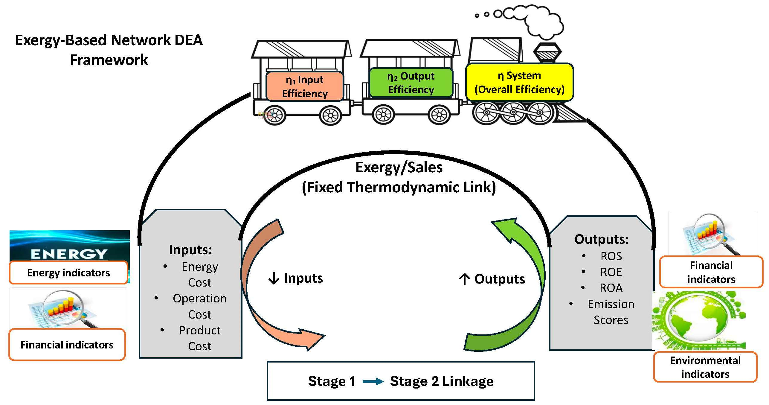
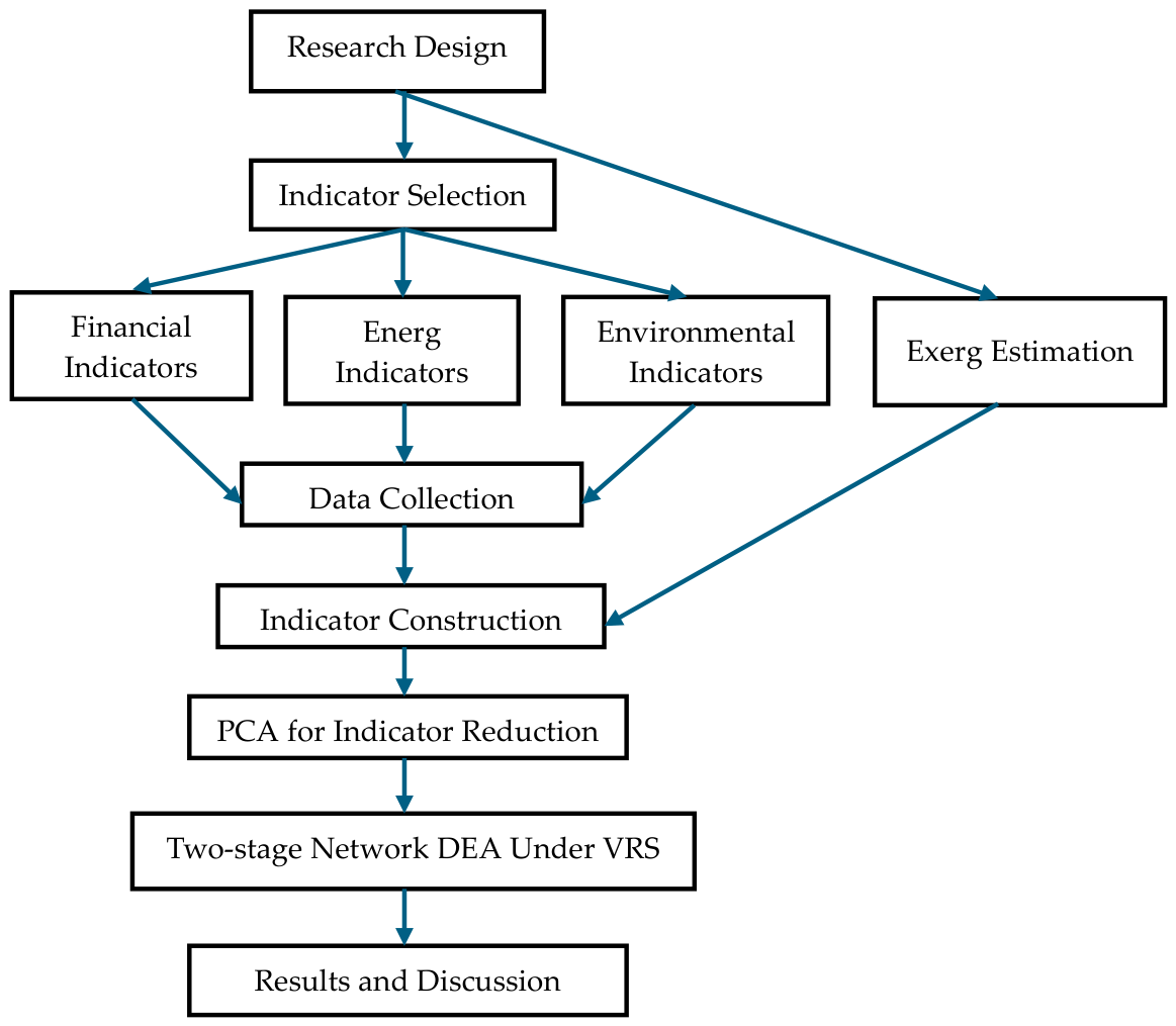
Principal Component Analysis (PCA) was applied to reduce the dimensionality of financial, energy, and environmental indicators by capturing their joint variation. As shown in

Table 12. Eigenvalues and cumulative explained variance of principal components.

Component	Eigenvalue	Explained Variance (%)	Cumulative Variance (%)
PC1	7.863	23.297	23.297
PC2	4.677	13.859	37.157
PC3	3.944	11.687	48.844
PC4	3.418	10.128	58.971
PC5	2.445	7.245	66.216
PC6	2.006	5.944	72.161
PC7	1.745	5.171	77.331
PC8	1.456	4.315	81.647

, the first eight principal components account for over 80% of the total variance, indicating that most of the information in the original variables is preserved in the reduced representation. Accordingly, these components were retained for subsequent analysis. This dimensionality reduction enhances the robustness of the efficiency model by mitigating multicollinearity and improving the discriminatory power of the DEA framework.

In addition, PCA loadings were analyzed to identify the dominant indicators underlying each principal component. Indicators with the highest absolute loadings were used to interpret the economic meaning of each component and to determine whether they primarily reflect financial, energy, or environmental performance dimensions.

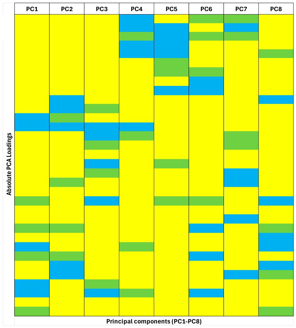
Figure 2 presents the distribution of absolute loadings, highlighting the relative contribution of each indicator category across components.

The results reveal distinct patterns across components. PC1, PC2, PC3, and PC8 are predominantly driven by financial indicators. In contrast, PC4 is mainly characterized by energy and environmental variables. PC5 is primarily energy-oriented, with a notable contribution from key financial indicators. PC6 reflects a mixed structure with substantial environmental and financial contributions, while PC7 exhibits a more balanced combination of financial, energy, and environmental indicators. The dominance of financial indicators across several principal components suggests that financial variables remain a major source of heterogeneity among firms, reflecting substantial differences in firms’ profitability structures and financial performance patterns.

Moreover, PCA scores provide the relative positioning of each industry with respect to the retained principal components.

Table 13. Sector-level average absolute PCA scores by component group (financial, energy, environmental and mixed).

Sector	PC1 3,8 (Fin)	PC4 (En/Env)	PC5 (En/Fin)	PC6 (Env/Fin)	PC7 (Mix)
Automobiles and Parts	0.574	0.050	0.612	0.635	0.640
Construction and Materials	0.800	0.765	0.027	0.995	0.026
Electricity	0.590	2.695	2.765	0.400	0.693
Food Producers	0.702	0.454	0.007	0.066	1.566
General Industrials	0.569	0.131	0.282	0.084	1.275
Industrial Materials	1.028	4.634	2.774	0.500	0.489
Industrial Metals and Mining	0.577	0.476	0.024	0.376	0.562
Industrial Support Services	0.909	0.006	0.595	1.844	1.682
Industrial Transportation	1.082	0.370	0.327	0.190	1.741
Media	0.812	0.611	0.133	0.180	1.028
Real Estate Investment and Services	1.374	1.384	1.112	0.006	1.734
Retailers	1.069	1.833	1.203	3.003	0.413
Software and Computer Services	0.740	1.060	0.074	0.142	2.891
Oil, Gas and Coal	0.418	0.299	0.026	0.707	0.065
Personal Care, Drug and Grocery Stores	0.996	0.185	0.869	0.983	0.297
Pharmaceuticals and Biotechnology	1.244	1.252	0.063	0.623	0.093
Telecommunications Service Providers	0.707	0.069	2.324	0.952	1.038
Travel and Leisure	1.484	0.814	0.519	1.430	0.152

Note: Fin = Financial; En = Energy; Env = Environmental; Mix = Mixed.

reports sector-level average absolute PCA scores, aggregated by the dominant loading structure for each component (financial, energy, environmental, or mixed). Higher magnitudes indicate a stronger alignment of each sector with the corresponding performance dimension, enabling the identification of predominant sectoral orientations.

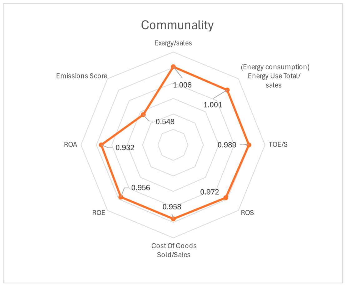
The selection of input, link, and output indicators for the Network DEA model was not arbitrary, but followed a structured, data-driven, and conceptually grounded approach. First, a Principal Component Analysis (PCA) was conducted to examine the contribution of candidate indicators across the retained components, ensuring that only variables with high communalities were retained. As illustrated in Figure 3, most selected indicators exhibit high communality values, confirming their ability to capture the dataset’s dominant variance structure.

From a managerial and operational perspective, the input indicators—Energy Use Total to Sales, TOE per Sales, and Cost of Goods Sold to Sales—represent controllable factors that firms can actively manage and optimize, particularly in the context of energy–cost management and operational efficiency. The Exergy-to-Sales ratio was selected as the link variable, as it integrates physical energy efficiency with economic scale, enabling the transmission of energy performance effects from operational inputs to financial and environmental outputs within the network.

Finally, financial performance indicators (ROS, ROE, and ROA) and the Emissions Score were selected as outputs to capture both economic and environmental outcomes. Although the Emissions Score exhibits a relatively lower communality value (0.548) compared to other indicators, its inclusion is justified by its critical environmental relevance and its role in reflecting sustainability-oriented performance, consistent with the recent literature on energy, exergy, and environmental efficiency assessment.

Following the PCA-based dimensionality reduction and indicator selection process, the retained variables were incorporated into a two-stage Network DEA framework. While PCA ensured that the selected indicators captured the dominant variance structure of the dataset, Network DEA enables the evaluation of operational and financial efficiency within an interconnected production structure. This integrated approach enables the assessment of how energy- and cost-related inputs are transformed into financial and environmental outcomes through intermediate link variables.

3.3. Network DEA Results: Baseline Scenario

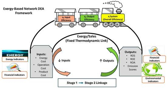
Following the PCA-based indicator selection, the retained variables were incorporated into a two-stage Network DEA model. Unlike the standard DEA framework, the proposed structure explicitly captures the internal production process. In Stage 1, energy- and cost-related inputs (Energy Use Total/Sales, TOE/S, Cost of Goods Sold/Sales) are transformed into an intermediate link variable (Exergy/Sales), which serves as the output of Stage 1 and the input of Stage 2, transmitting efficiency effects between the two stages without altering its intrinsic definition. In Scenario I, only financial indicators (ROS, ROE, ROA) are considered as outputs. In Scenario II, the Emissions Score is additionally incorporated as an environmental output to account for sustainability performance. This structure enables the assessment of operational (energy–cost) efficiency, financial efficiency, and interaction within an integrated network framework.

The model is estimated under Variable Returns to Scale (VRS) assumptions. System efficiency is computed as the geometric mean of Stage 1 and Stage 2 efficiencies, ensuring balanced performance across both sub-processes. To satisfy DEA non-negativity requirements, a constant shift was applied to standardized variables when necessary. The analysis includes 45 decision-making units (DMUs).

For clarity, the empirical findings are presented in a stage-wise sequence. Since the environmental indicator is introduced only in Stage 2 under Scenario II, Stage 1 results remain identical across scenarios. Accordingly, Stage 1 efficiencies are reported first, followed by Stage 2 and overall system efficiency under both scenarios. In addition to efficiency scores, target analysis is conducted to provide managerial insights. Stage 1 targets reflect the proportional reduction required in energy- and cost-related inputs, while Stage 2 targets indicate the expansion needed in financial outputs and, under Scenario II, environmental performance. This structure enables the assessment of how incorporating environmental performance reshapes firms’ improvement paths.

3.3.1. Stage 1: Operational (Energy–Cost) Efficiency

In Stage 1, an input-oriented VRS Network DEA model was applied to evaluate the operational efficiency of firms in transforming energy- and cost-related inputs into the intermediate link variable (Exergy/Sales). This stage assesses how efficiently companies manage energy intensity and cost structures while maintaining the same thermodynamic performance level. Stage 1 efficiency reflects the minimum proportional reduction in all inputs required to maintain the observed level of the intermediate link variable.

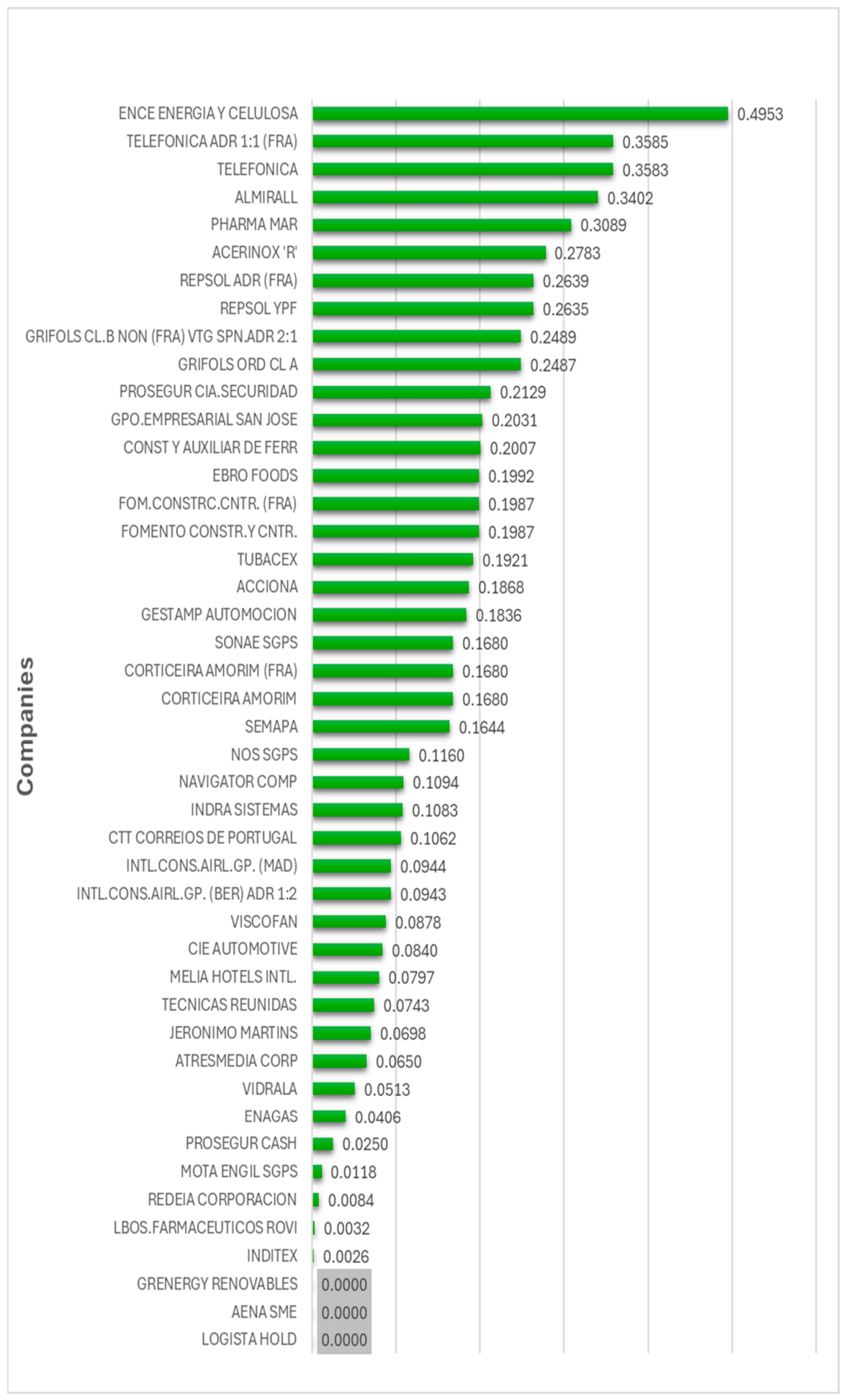
The results indicate that only a subset of firms lies on the Stage 1 efficiency frontier (efficiency score = 1), demonstrating optimal management of energy and cost inputs. Firms with efficiency scores below unity exhibit proportional input excesses, implying potential reductions in energy consumption and cost intensity without affecting the intermediate link performance. Figure 4 illustrates the distance of each firm from the efficiency frontier. The distance from the efficiency frontier was calculated as (1 − Efficiency Score). Therefore, values close to zero indicate firms operating near the efficiency frontier, while small negative values may occur due to numerical precision and rounding to five decimal places. Firms with larger distances require greater proportional reductions in inputs to reach the frontier, whereas firms close to zero distance operate near best-practice performance. Due to numerical precision, some efficiency scores slightly exceed unity (e.g., 1.00005). Therefore, firms were considered strictly efficient only when the efficiency score was equal to one at full numerical precision (without rounding).

Based on strict numerical precision, eight firms are identified as fully efficient in Stage 1. This finding indicates that only a limited subset of firms achieves optimal energy–cost management relative to their thermodynamic performance level. The limited number of fully efficient firms suggests substantial heterogeneity in firms’ ability to manage energy- and cost-related inputs while maintaining the same thermodynamic performance level. This may reflect differences in operational structures, energy management practices, and sectoral exposure to energy intensity. Firms located farther from the frontier are likely to face greater inefficiencies in balancing energy consumption, operational costs, and exergy-related performance.

Table 14. Stage 1 Efficiency Scores and Sector Classification.

Firms	Sector	Stage 1 Efficiency
INDRA SISTEMAS	Software and Computer Services	1
AENA SME	Industrial Transportation	1
ENAGAS	Oil, Gas and Coal	1
ENCE ENERGIA Y CELULOSA	Industrial Materials	1
GREENERGY RENOVABLES	Electricity	1
LOGISTA HOLD	Industrial Transportation	1
PHARMA MAR	Pharmaceuticals and Biotechnology	1
REDEIA CORPORACION	Electricity	1

reports the Stage 1 efficiency scores along with firms’ sectoral classification. Eight firms are identified as fully efficient (efficiency score = 1), indicating optimal energy–cost management relative to their thermodynamic performance level.

3.3.2. Stage 2: Financial and Environmental Output Efficiency

In Stage 2, an output-oriented VRS Network DEA model was employed to evaluate how efficiently firms generate financial performance (ROS, ROE, and ROA) given the observed level of the intermediate link variable (Exergy/Sales). The link variable, carried over from Stage 1, acts as a fixed input in this stage. The objective is to determine the proportional expansion required in financial outputs to maintain the same Exergy/Sales level and reach the efficiency frontier.

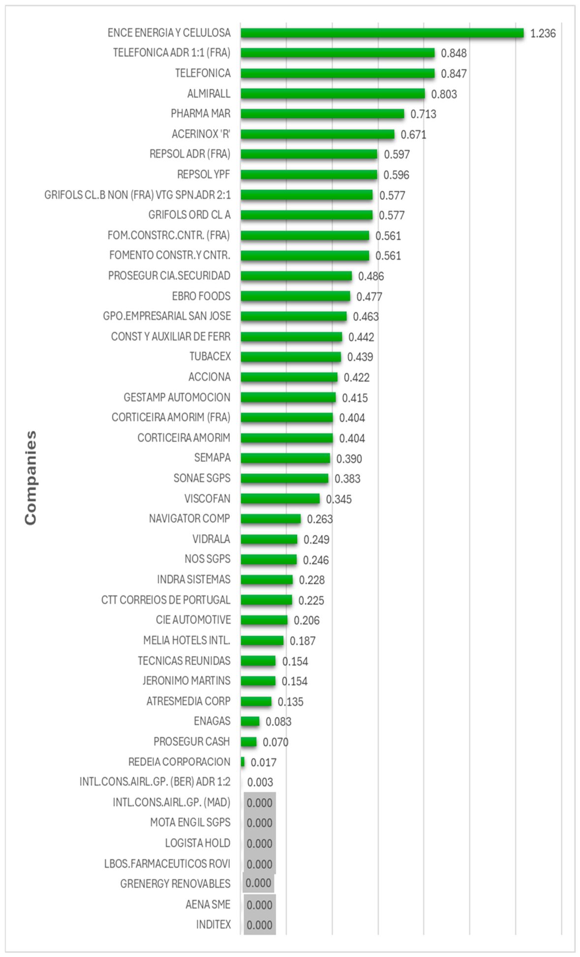
An efficiency score of 1 represents full efficiency, meaning the firm maximizes its financial performance given its observed Exergy/Sales ratio. Firms with efficiency scores lower than 1 are located below the frontier and require proportional increases in their financial outputs to attain best-practice performance. Due to numerical precision considerations, firms were classified as strictly efficient only when their efficiency score was exactly equal to 1 at full computational precision. Based on this criterion, seven firms were identified as fully efficient in Stage 2. The distance to the frontier was computed as (Efficiency − 1) and is illustrated in Figure 5.

Figure 5 shows a wider dispersion of distances compared to Stage 1, indicating greater variability in firms’ financial performance. This broader dispersion may reflect differences in firms’ financial structures, market conditions, and sectoral profitability patterns, which introduce greater variability into financial efficiency assessment compared with operational energy–cost performance. Firms with larger distances require greater proportional improvements in financial indicators to achieve efficiency. The results reveal substantial heterogeneity across firms, indicating that strong operational (energy–cost) efficiency in Stage 1 does not necessarily translate into superior financial performance in Stage 2. To facilitate interpretation of the Stage 2 results under Scenario I (financial outputs only),

Table 15. Stage 2 Efficiency Scores and Sector Classification (Scenario I).

Firms	Sector	Stage 2 Efficiency
INDITEX	Retailers	1
AENA SME	Industrial Transportation	1
GREENERGY RENOVABLES	Electricity	1
LBOS.FARMACEUTICOS ROVI	Pharmaceuticals and Biotechnology	1
LOGISTA HOLD	Industrial Transportation	1
MOTA ENGIL SGPS	Construction and Materials	1
INTL.CONS.AIRL.GP. (MAD)	Travel and Leisure	1

reports the firms identified as fully efficient (efficiency score = 1) together with their industry classification. This presentation allows a clearer comparison with the extended model under Scenario II and highlights structural differences across stages. Notably, not all firms efficient in Stage 1 remain efficient in Stage 2, indicating that strong operational (energy–cost) efficiency does not automatically translate into superior financial performance.

To examine the effect of incorporating environmental performance into the evaluation framework, Stage 2 efficiency scores were recalculated under Scenario II, in which the Emissions Score was included as an additional output. Including the environmental indicator altered the efficiency classification of several firms. Specifically, the number of fully efficient firms increased from 7 in Scenario I to 9 in Scenario II, indicating that environmental performance strengthened the relative positions of certain companies within the network structure. Interestingly, the two firms that reached full efficiency under Scenario II, the Software and Computer Services sector (INDRA SISTEMAS) and the Oil, Gas, and Coal sector (ENAGAS), respectively, were already efficient in Stage 1. This suggests that strong operational (energy–cost) efficiency, when complemented by favorable environmental performance, enhances firms’ ability to reach the financial efficiency frontier in the extended model.

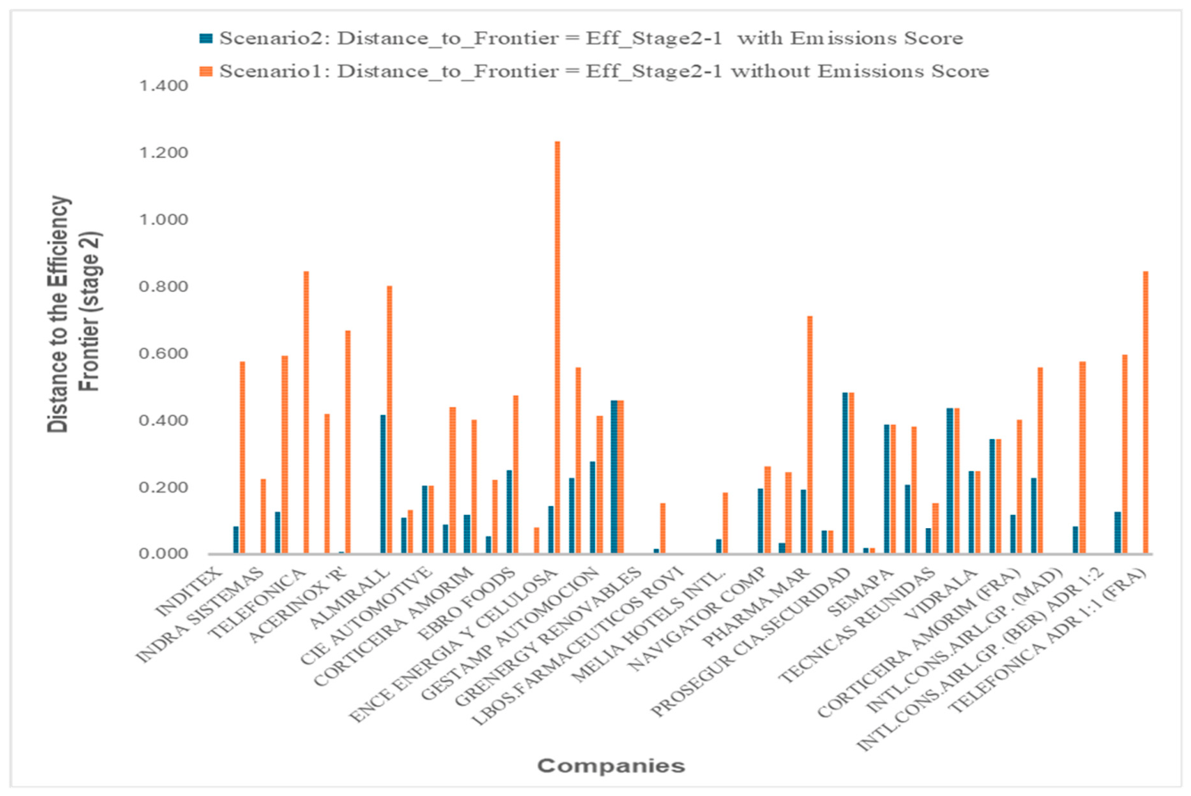
Comparative inspection (Figure 6) indicates that incorporating environmental performance reduces inefficiency for a large proportion of firms, shifting them closer to the frontier. However, for some firms, efficiency levels remain unchanged, suggesting limited sensitivity to environmental factors. These findings highlight that incorporating environmental dimensions can reshape firms’ improvement pathways by recognizing strengths that are not captured when only financial outputs are considered.

To provide a clearer structural comparison between Scenario I and Scenario II,

Table 16. Reclassification of Firms After Incorporating Environmental Output in Stage 2.

Classification	Scenario I	Scenario II	Change
Fully efficient firms	7	9	+2
Inefficient firms (total)	38	36	−2
Inefficient—unchanged	-	9	+9
Inefficient—improved (distance reduced)	-	27	+27
Total firms	45	45	-

summarizes the reclassification of firms after incorporating the environmental output. The table reports the number of fully efficient firms and the distribution of inefficient firms by whether their efficiency status improved or remained unchanged.

The results show that incorporating the environmental indicator increased the number of fully efficient firms from 7 to 9, while reducing inefficient firms from 38 to 36. Notably, 27 firms improved their positions relative to the frontier, highlighting the positive role of environmental performance in enhancing efficiency, while nine showed no change in efficiency. Importantly, the incorporation of the environmental indicator did not cause any previously efficient firms to become inefficient.

3.3.3. System: Financial and Environmental Output Efficiency

System efficiency was computed by integrating the efficiencies of the two stages within the Network DEA framework. Stage 1 captures operational (energy–cost) efficiency relative to the intermediate link variable (Exergy/Sales), whereas Stage 2 assesses financial efficiency conditional on the thermodynamic performance achieved in Stage 1.

Overall system performance was obtained using the geometric mean of stage-specific efficiencies:

$${\mathrm{E}}_{\mathrm{S}\mathrm{y}\mathrm{s}\mathrm{t}\mathrm{e}\mathrm{m}}=\sqrt{{\mathrm{E}}_{\mathrm{S}\mathrm{t}\mathrm{a}\mathrm{g}\mathrm{e}1}\times {\mathrm{E}}_{\mathrm{S}\mathrm{t}\mathrm{a}\mathrm{g}\mathrm{e}2}}$$

(1)

The geometric mean ensures balanced performance across both stages and avoids overestimation when one stage performs strongly while the other underperforms, making it particularly suitable for interconnected network structures.

The results indicate that only a limited number of firms lie on the system efficiency frontier, reflecting strong integrated performance across both operational and financial dimensions. Firms with system efficiency below unity exhibit inefficiencies in at least one stage, requiring improvements in either energy–cost management (Stage 1) or financial output expansion (Stage 2).

To measure deviation from the frontier symmetrically, the absolute distance from full efficiency was calculated as:

$$Distance=\lceil {\mathrm{E}}_{\mathrm{S}\mathrm{y}\mathrm{s}\mathrm{t}\mathrm{e}\mathrm{m}}-1\rceil$$

(2)

Figure 7 presents the absolute distance of each firm from the system efficiency frontier. Only three firms exhibit zero distance, confirming full integrated efficiency across both stages. The remaining firms show positive deviations, indicating inefficiencies in at least one stage that constrain overall system performance. Firms with shorter distances operate closer to best-practice integrated performance, whereas larger distances reflect greater imbalances between operational and financial efficiency.

To assess the impact of environmental performance at the system level, efficiency scores were recalculated under Scenario II. The number of firms on the system efficiency frontier increased from 3 to 5, indicating that incorporating the environmental output enhances firms’ ability to achieve fully integrated operational–financial–environmental efficiency. While some firms remained unchanged, many reduced their distance to the frontier, reflecting improved overall performance consistency across stages.

Table 17. Reclassification of Firms After Incorporating Environmental Output in System.

Classification	Scenario I	Scenario II	Change
Fully efficient firms	3	5	+2
Inefficient firms (total)	42	40	−2
Inefficient—unchanged	-	13	+13
Inefficient—improved (distance reduced)	-	27	+27
Total firms	45	45	-

presents a comparative overview of firms’ system-level classifications under both scenarios. Unlike Stage 2, the system perspective captures the combined effect of operational and financial efficiencies, reflecting structural changes in overall performance positioning following the inclusion of the environmental output.

At the integrated level, the number of firms achieving full system efficiency increased from 3 to 5 after incorporating the environmental indicator. Although most firms remained below the frontier, a substantial proportion moved closer to best-practice performance. Thirteen firms have no change, suggesting that environmental performance alone is insufficient to offset inefficiencies originating from either Stage 1 or Stage 2. Overall, the results indicate that environmental considerations improve alignment between operational and financial performance, but do not uniformly alter firms’ relative positions.

An important observation is that the 27 firms whose distance to the frontier decreased in Stage 2 under Scenario II are the same firms that exhibit a reduction in system-level distance. This one-to-one correspondence confirms that improvements driven by the environmental output in Stage 2 are consistently transmitted to the overall system efficiency through the geometric aggregation structure. This finding indicates that environmental performance enhancements are not isolated at the sub-process level but effectively translate into integrated efficiency gains.

The very small difference between the average improvement in Stage 2 (67.66%) and the system level (68.58%) further confirms the strong transmission effect of environmental performance through the geometric aggregation mechanism of the Network DEA model. This numerical proximity indicates that improvements generated in Stage 2 are almost proportionally reflected in overall system efficiency.

3.3.4. Target: Energy and Cost Input Efficiency

Target values in Stage 1 are calculated exclusively for inefficient firms. The input-oriented VRS Network DEA model determines the minimum proportional reductions in energy- and cost-related inputs required to reach the Stage 1 efficiency frontier. The intermediate link variable (Exergy/Sales) is treated as a fixed carry-over component and is not directly optimized in this stage.

Accordingly, target adjustments reflect proportional input contractions based on each firm’s efficiency score, indicating the extent to which firms must reduce operational resource usage to achieve best-practice performance without altering the intermediate linkage structure.

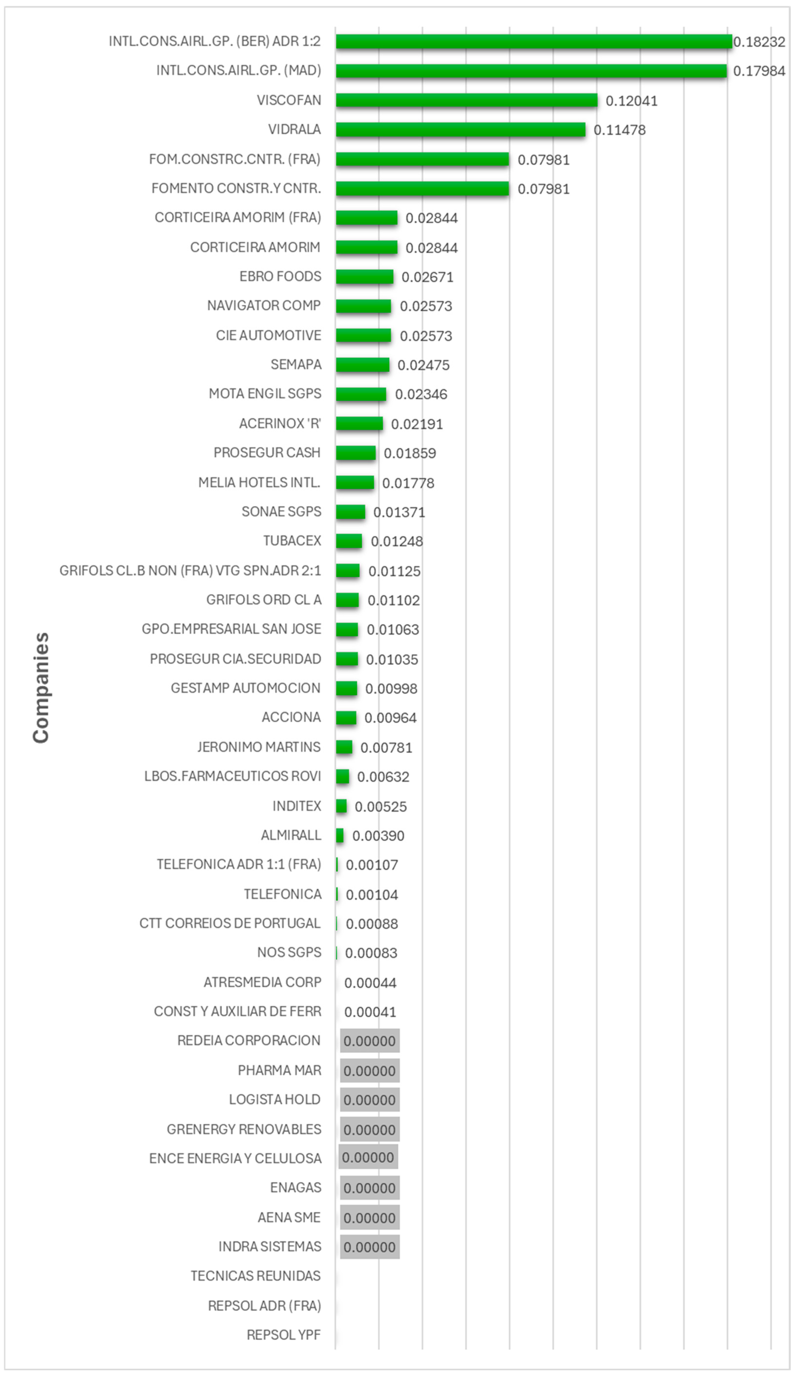
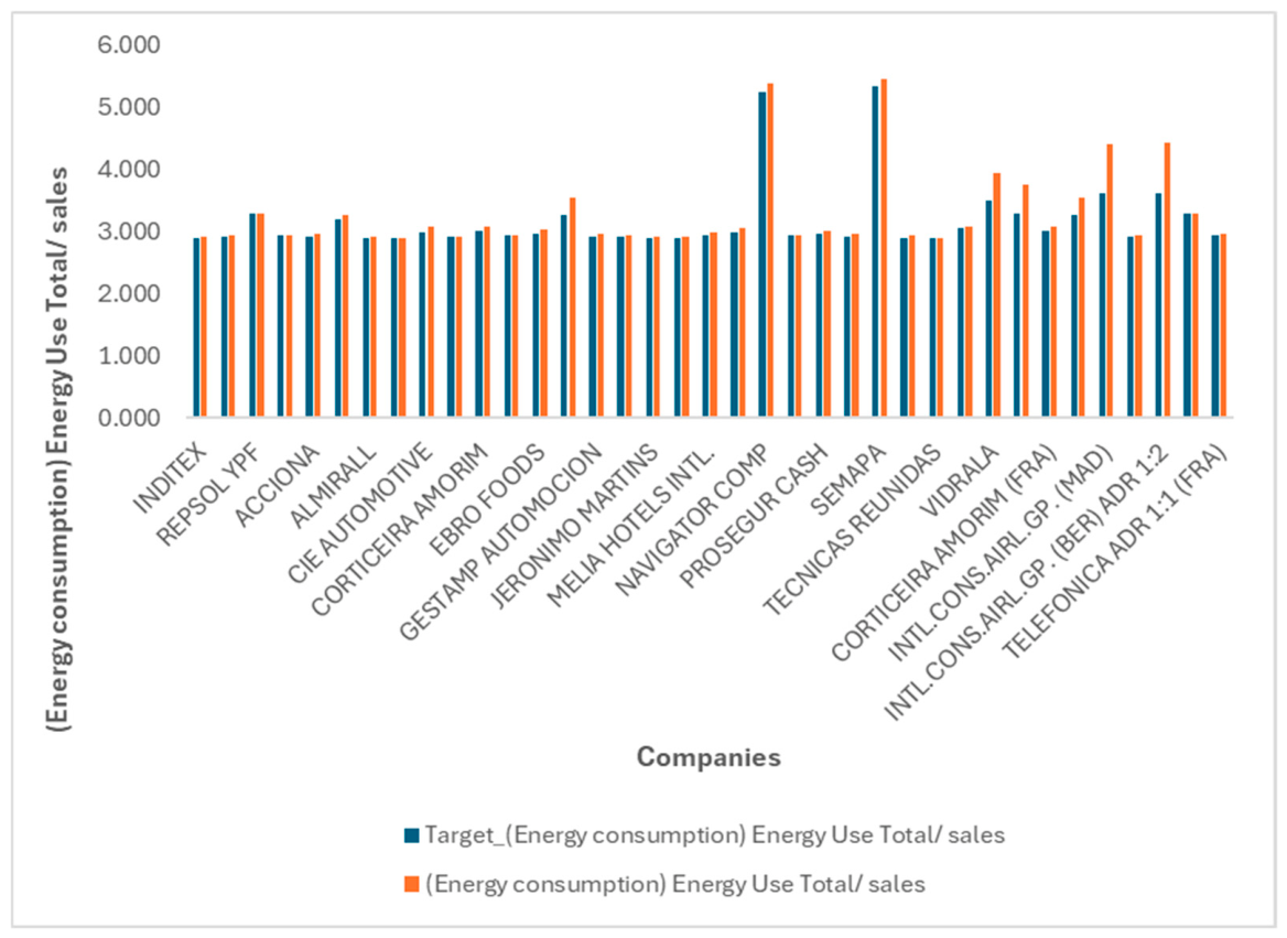
The comparison between the observed and target energy consumption-to-sales ratios indicates that inefficient firms must reduce their energy intensity to reach the Stage 1 efficiency frontier. On average, the required reduction across the 37 inefficient firms is approximately 3%, with a standard deviation of 4.70%, indicating substantial heterogeneity in adjustment requirements. However, adjustment levels vary substantially, ranging from 0.005% to 18.23%. The largest reduction is associated with INTL.CONS.AIRL.GP. (BER) ADR 1:2, reflecting significant inefficiency in energy utilization, while minimal adjustments correspond to firms already operating close to the frontier. Figure 8 illustrates the gap between observed and target ratios.

As shown in Figure 8, target ratios are consistently lower than observed values for inefficient firms, confirming the proportional input reductions required to reach the Stage 1 efficiency frontier.

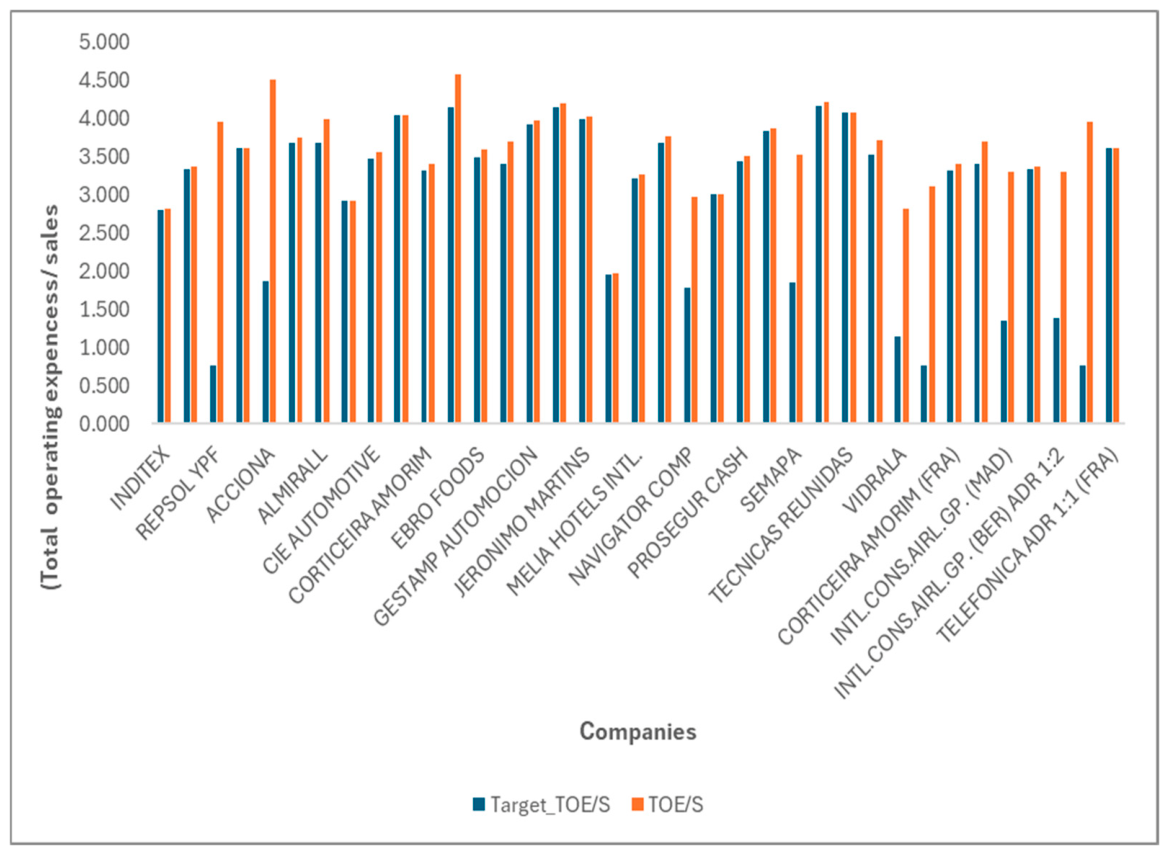
The target analysis for the Total Operating Expenses-to-Sales (TOE/S) ratio reveals substantially larger adjustment requirements than those observed for energy consumption-to-sales. On average, inefficient firms must reduce their TOE/S ratio by approximately 16.92% to reach the Stage 1 efficiency frontier, with required reductions ranging from 0.005% to 80.98%. The largest adjustment is observed for Repsol YPF, indicating a significant imbalance between operating expenses and revenue, while minimal adjustments are observed for firms already operating close to the frontier. As shown in Figure 9, target TOE/S values are consistently lower than observed levels. Compared with the average 3% reduction in energy consumption-to-sales required, these results suggest that cost inefficiency is the primary source of Stage 1 performance gaps. This finding suggests that, for many firms, operational inefficiency is driven more by cost structure and expense management than by excessive energy consumption alone. In other words, firms may operate with relatively acceptable energy intensity while still remaining inefficient due to unfavorable operating or production cost patterns.

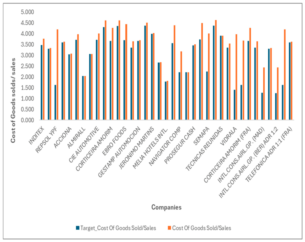
The target assessment for the Cost of Goods Sold-to-Sales (COGS/S) ratio indicates substantial adjustment requirements among inefficient firms in Stage 1. On average, firms must reduce their COGS/S ratio by approximately 15.48% to reach the efficiency frontier, with required reductions ranging from 0.005% to 64.88%. As shown in Figure 10. The largest adjustment is observed for VIDRALA, operating in the General Industrials sector, reflecting a significant misalignment between production costs and revenue, while minimal reductions for Técnicas Reunidas, from the Oil, Gas and Coal sector, suggest operation near the optimal cost structure.

Overall, the wide dispersion in required adjustments highlights heterogeneous cost structures across industries and underscores the critical role of production cost management in driving Stage 1 inefficiency. The similarity between average adjustments in TOE/S and COGS/S further suggests that operational cost components jointly account for many input-side inefficiencies. Overall, the results indicate that Stage 1 inefficiencies are driven more by operational and production cost factors than by energy consumption inefficiencies alone.

These findings collectively indicate that, while energy inefficiency is relatively limited, operational cost components—particularly production costs—dominate inefficiencies in Stage 1.

3.3.5. Target: Financial and Environmental Output Efficiency

Prior to incorporating the environmental variable, Stage 2 results show that 38 out of the 45 firms are inefficient, with only seven firms located on the efficiency frontier. In this stage, the intermediate link variable (Exergy-to-Sales) from Stage 1 remains fixed and is not optimized.

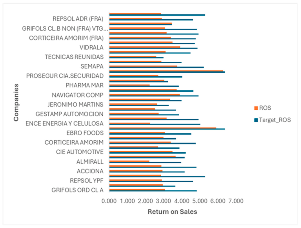
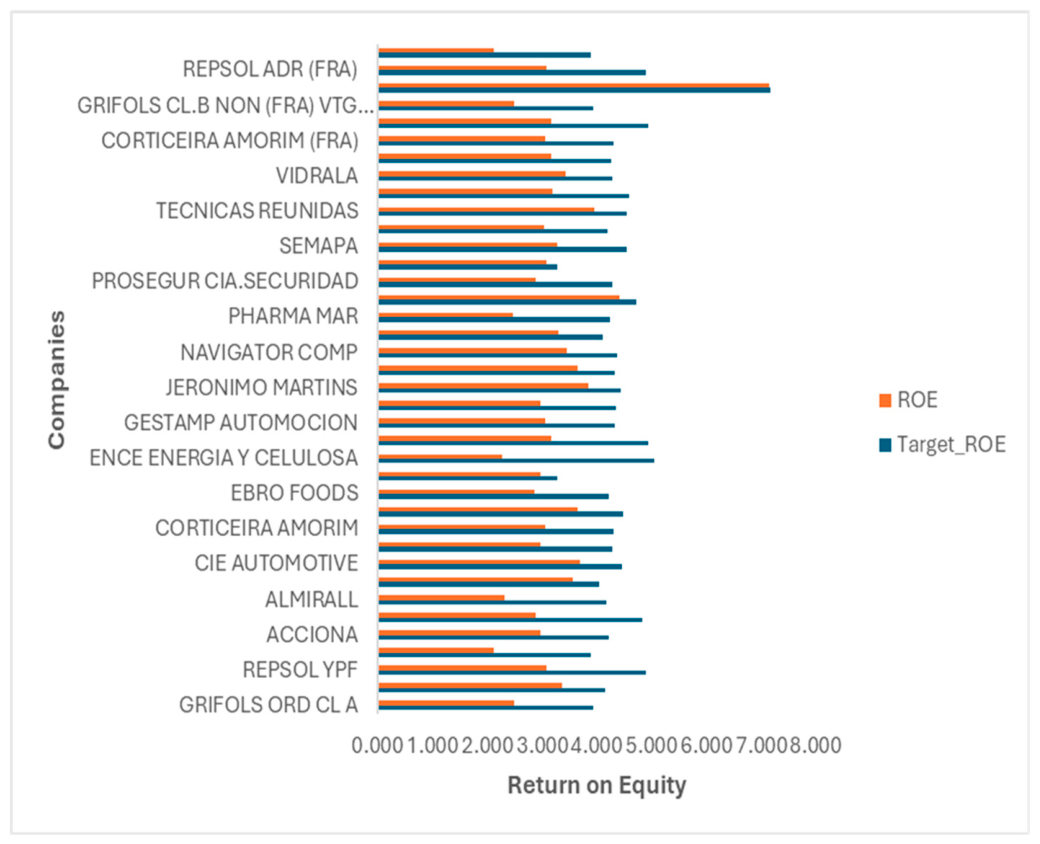
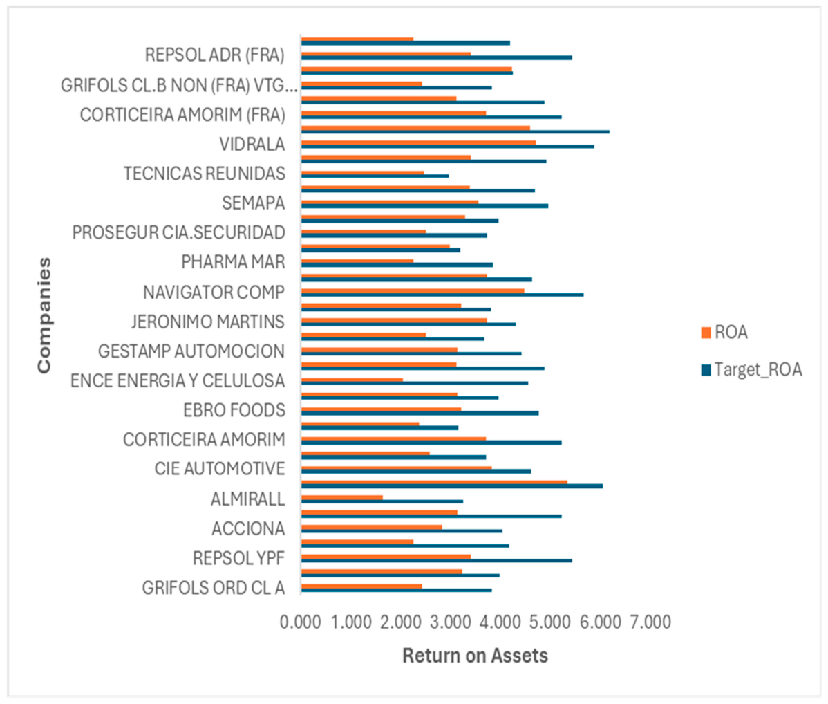
Target values are therefore defined for the financial output indicators (ROS, ROE, and ROA) of the inefficient firms. On average, firms must increase ROS by 42.02%, ROE by 41.94%, and ROA by 43.67% to reach the Stage 2 efficiency frontier. The required improvements vary substantially, ranging from 0.33% to 123.58%, while the similarity in average adjustment levels across ROS, ROE, and ROA suggests that financial inefficiency is broadly distributed across multiple dimensions of firm performance rather than concentrated in a single profitability indicator.

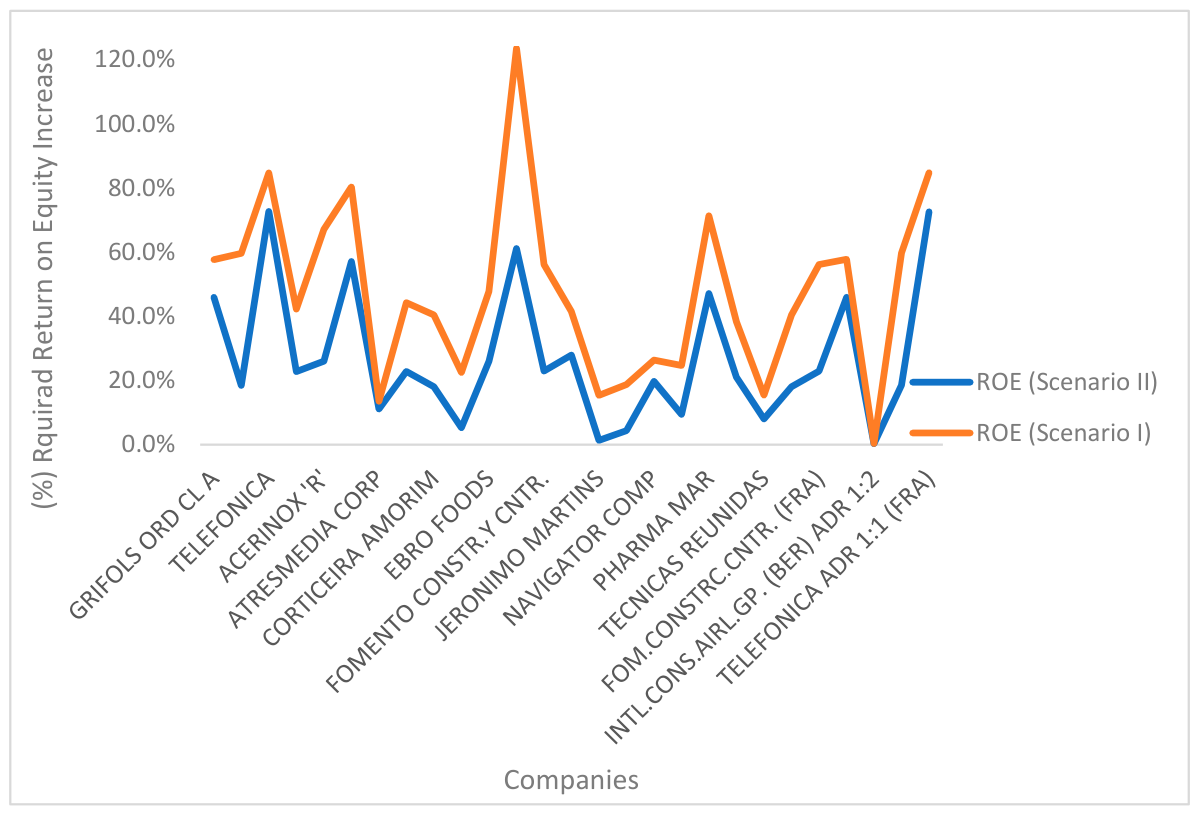
Given that the Exergy-to-Sales ratio remains unchanged, the required increases in financial outputs reflect the extent to which firms must enhance profitability without modifying the energy-to-sales relationship established in Stage 1. Figure 11, Figure 12 and Figure 13 illustrate the comparison between observed and target values of the financial output indicators in Stage 2 prior to the incorporation of the environmental variable. The visible gap between observed and target levels highlights the magnitude of financial performance improvement required for inefficient firms to reach the efficiency frontier while preserving a fixed Exergy-to-Sales ratio.

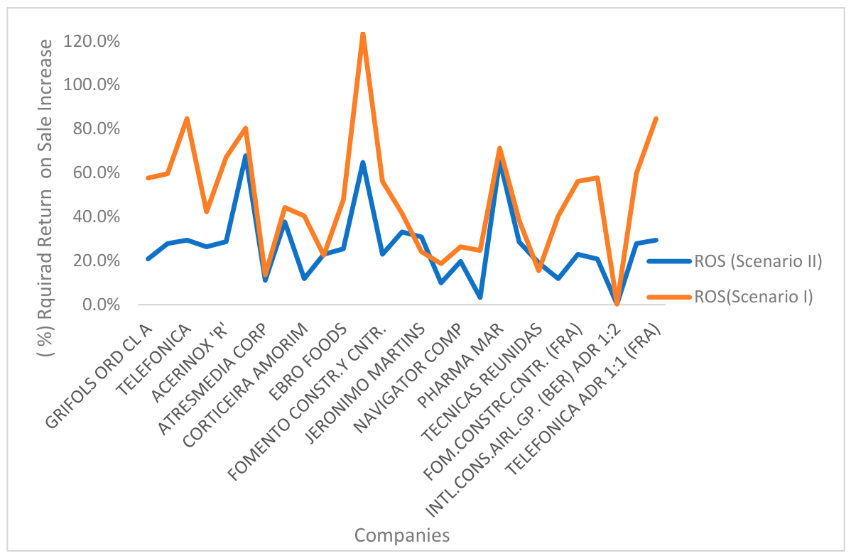
After incorporating the environmental variable (Emissions Score), the number of inefficient firms decreases from 38 to 36, with nine firms remaining fully efficient. The analysis, therefore, focuses on the remaining 27 firms. As illustrated in Figure 14, the required ROS increase varies substantially across firms, ranging from 0.30% to 123.58%. Compared to the baseline scenario, the inclusion of the environmental indicator significantly alters both the distribution and magnitude of the required financial adjustments, indicating that part of the previously observed financial inefficiency appears to be associated with environmental performance considerations. For these 27 firms, the average required ROS increase declines from 48.11% to 26.68% after incorporating the environmental dimension. This substantial reduction indicates that accounting for environmental performance reduces the estimated financial inefficiency. The narrowing gap between observed and target values implies that firms move closer to the efficiency frontier when environmental performance is explicitly considered.

For the 27 remaining inefficient firms, the inclusion of the environmental variable leads to a substantial reduction in the required ROE adjustments. Prior to incorporating the Emissions Score (Scenario I), firms required an average ROE increase of 47.79% to reach the Stage 2 efficiency frontier. After incorporating the environmental dimension (Scenario II), this average declines to 26.93%. As illustrated in Figure 15, the gap between observed and target values narrows under Scenario II, indicating that firms approach the efficiency frontier with comparatively smaller financial improvements when environmental performance is explicitly incorporated into the model.

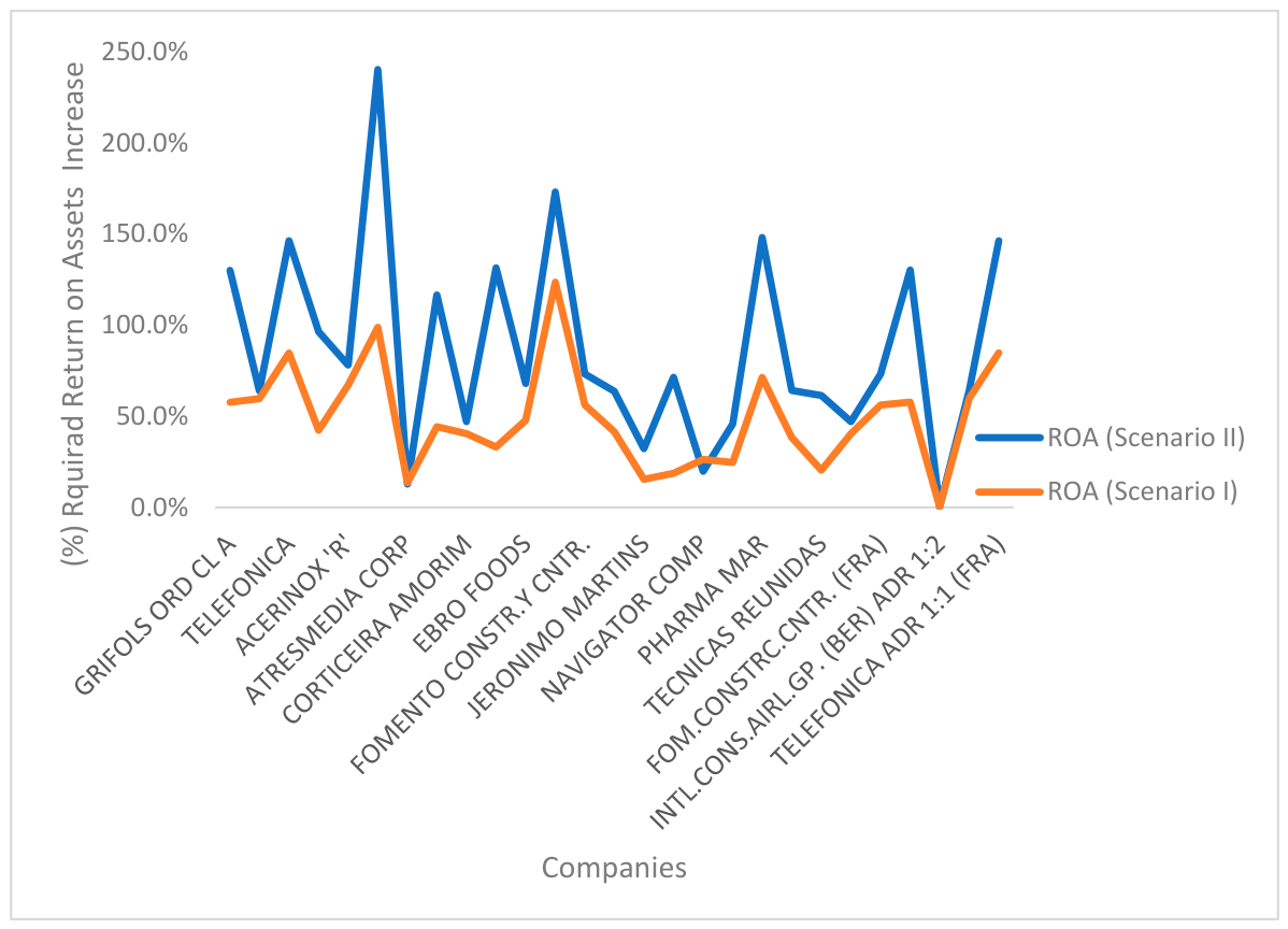
In contrast to ROS and ROE, the inclusion of the environmental variable (Emissions Score) leads to a substantial increase in the required ROA adjustments. For the 27 firms that remain inefficient, the average required ROA increase rises from 49.05% under Scenario I to 86.83% under Scenario II (Figure 16). The dispersion of adjustments also expands considerably, with the maximum required increase rising from 123.58% to 240.35%, while the minimum adjustment remains nearly unchanged (0.33% versus 0.31%).

This pattern indicates that incorporating the environmental dimension reshapes the efficiency frontier, making asset utilization requirements more stringent. Under the augmented framework, firms are benchmarked not only against financially strong peers but also against firms that jointly exhibit strong financial and environmental performance.

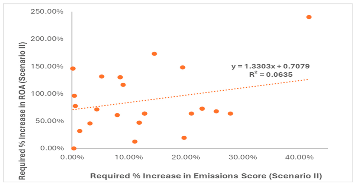
Importantly, no clear monotonic or direct relationship is observed between the required increase in Emissions Score and the magnitude of the required ROA adjustment. Some firms with minimal environmental gaps still require substantial improvements in ROA. This suggests that the environmental variable does not directly determine financial performance adjustments; rather, its inclusion alters the composition of the reference set and reconfigures the multi-dimensional efficiency frontier. Consequently, under Scenario II, achieving efficiency in the asset-return dimension requires larger proportional adjustments than under the purely financial specification.

Figure 17 illustrates the relationship between the required percentage increase in ROA and the required improvement in the Emissions Score under Scenario II. Although the estimated slope is positive, the very low coefficient of determination (R² = 0.0635) indicates a weak linear association between the two variables. Moreover, the slope coefficient is not statistically significant (p = 0.205), suggesting that the observed positive relationship is not statistically distinguishable from zero. This suggests that the substantial increase in required ROA adjustments after incorporating the environmental dimension is not directly driven by the magnitude of the environmental gap. Instead, the inclusion of the environmental variable reshapes the efficiency frontier and alters the structure of the reference set, thereby imposing stricter asset-efficiency requirements on certain firms. While ROS and ROE consistently move closer to the efficiency frontier under Scenario II, the opposite pattern observed for ROA reflects a structural shift in benchmarking criteria rather than a direct effect of environmental performance. This highlights the importance of considering multi-dimensional interactions when interpreting efficiency adjustments.

These findings suggest that firms aiming to improve sustainability performance may experience heterogeneous impacts across different financial dimensions, particularly in asset utilization efficiency.

3.4. Comparative Analysis and Managerial Implications

The inclusion of the environmental output does not directly improve or impair financial performance. Instead, it redefines the efficiency frontier by altering the reference set against which firms are evaluated. Consequently, financial indicators respond asymmetrically to this change: ROS and ROE require relatively smaller adjustments under Scenario II, whereas ROA requires substantially larger improvements. This may indicate that asset-utilization efficiency is more sensitive to the redefinition of the efficiency frontier after incorporating environmental performance, particularly because asset-related measures are more strongly affected by structural differences across firms.

This pattern indicates that environmental integration reshapes benchmarking relationships rather than generating mechanical performance effects. This interpretation is broadly consistent with the recent sustainability-accounting literature emphasizing that changes in environmental accounting boundaries and responsibility attribution can reshape the relative positioning of actors within interconnected systems [101]. From this perspective, the asymmetric responses observed across ROS, ROE, and ROA may reflect structural changes in the multidimensional efficiency frontier following environmental integration.

ROS and ROE tend to converge toward the efficiency frontier, whereas ROA becomes more demanding under the redefined frontier. Overall, incorporating environmental performance modifies the benchmarking structure associated with financial efficiency assessment. These findings extend prior DEA-based studies on integrated sustainability and energy-efficiency assessment [102] by demonstrating that environmental integration changes firms’ relative financial positioning rather than producing uniform financial effects.

The Exergy-to-Sales ratio plays a crucial structural role in this framework. As a fixed intermediate link connecting thermodynamic performance to financial outcomes, it remains fixed across scenarios. Therefore, all estimated financial adjustments are based on an identical thermodynamic benchmark, ensuring that observed differences stem from frontier reconfiguration rather than changes in the intermediate stage.

From a managerial perspective, environmental integration affects firm positioning in a differentiated manner. The increase in the number of efficient firms and the reduction in average distance to the frontier suggest that sustainability considerations can enhance relative efficiency for a substantial number of firms, although not uniformly across financial dimensions. Managers should recognize that environmental performance reshapes competitive benchmarks, potentially easing some efficiency requirements while tightening others.

The results also suggest differentiated managerial implications across firm types. Firms exhibiting Stage 1 inefficiencies should primarily focus on improving operational and production cost structures, as energy-related inefficiencies appear comparatively limited. Since the Exergy-to-Sales ratio functions as a fixed intermediate link, these managerial adjustments are interpreted within a stable thermodynamic benchmarking structure. Firms that move closer to the efficiency frontier under Scenario II may benefit from leveraging environmental performance as a strategic competitive advantage. In contrast, firms requiring substantial ROA adjustments under the sustainability-augmented framework may need to improve asset utilization efficiency and capital allocation practices in order to remain competitive under increasingly integrated financial and environmental performance expectations.

At the policy level, embedding environmental metrics within performance systems grounded in physical production structures is essential. Linking sustainability indicators to thermodynamically anchored measures such as Exergy-to-Sales enables policymakers and analysts to move beyond purely symbolic ESG integration and capture the structural dynamics of firm performance.

Despite its contributions, this study presents several limitations that open avenues for future research. First, the analysis is based on a cross-sectional dataset for a single year (2023), which does not capture dynamic changes in firms’ efficiency over time. Future studies could extend the framework to panel data, enabling the assessment of efficiency dynamics and the impact of evolving energy and environmental policies.

Second, the sample is limited to firms operating in Portugal and Spain, which may constrain the generalizability of the findings. Expanding the analysis to a broader set of countries and institutional contexts would allow for cross-country comparisons and more robust policy insights. Moreover, the empirical sample was restricted to firms with sufficiently complete and consistent energy, environmental, and financial disclosures for 2023, which constrained the final number of observations included in the analysis.

Third, although the model integrates financial, energy, and environmental dimensions, the social dimension of sustainability is not included due to the lack of standardized and quantifiable indicators compatible with the Network DEA framework.

Future research could explore ways to incorporate social performance metrics, particularly as ESG data availability improves. Additionally, the use of a deterministic DEA approach does not account for statistical noise or measurement errors; thus, future work could consider stochastic or robust DEA extensions to enhance methodological rigor. While bootstrap DEA techniques could provide additional statistical inference regarding efficiency estimates, the present study focuses primarily on the structural and comparative properties of the proposed exergy-based Network DEA framework. The application of bootstrap DEA is acknowledged as a valuable extension for future research.

Finally, further research could explore alternative specifications of the intermediate link variable and investigate the integration of exergy-based indicators into corporate accounting and reporting systems, strengthening the practical applicability of the framework.

3.5. Sensitivity Analysis of Exergy Coefficients

To evaluate the robustness of the proposed framework with respect to uncertainty in the exergy conversion coefficients (ϕ), a sensitivity analysis was conducted by varying all sector-level ϕ coefficients by ±10%. Following each perturbation scenario, the exergy values were recalculated and the complete analytical procedure—including normalization, correlation analysis, PCA, and the two-stage Network DEA model—was re-estimated.

The results indicate that moderate variations in the ϕ coefficients do not materially affect the overall structure of the model. Although minor changes were observed in correlations involving the Exergy-to-Sales ratio, the PCA loading structure, retained components, and indicator selection remained unchanged across scenarios. Similarly, the Network DEA results exhibited strong stability. Firms identified as efficient under the baseline specification remained efficient under both perturbation scenarios, and the principal findings regarding the asymmetric behavior of ROS, ROE, and ROA under Scenario II were preserved.

These findings suggest that the proposed framework is robust to moderate variations in the exergy conversion assumptions adopted from the PFU-based literature.

4. Conclusions

This study develops an exergy-based two-stage Network DEA framework to evaluate firms’ efficiency by integrating financial, energy, and environmental performance dimensions within a unified analytical structure. The analysis addresses how incorporating energy and cost variables in Stage 1 and environmental performance in Stage 2 reshapes the structure of financial efficiency assessment, moving beyond isolated financial evaluation toward a multidimensional perspective grounded in physical production logic.

From a methodological perspective, the study demonstrates the value of integrating dimensionality reduction techniques, such as Principal Component Analysis (PCA), within a network DEA framework to address data complexity and multicollinearity. In this structure, Stage 1 captures energy-and cost-related inefficiencies, while Stage 2 reveals how environmental integration reshapes financial performance assessment, providing a more comprehensive understanding of the structural drivers of inefficiency across interconnected stages.

The findings show that incorporating environmental performance does not exert a uniform mechanical effect on financial indicators but instead redefines the efficiency frontier by altering the reference set. Under the sustainability-augmented scenario, ROS and ROE require smaller adjustments and move closer to the efficiency frontier, whereas ROA requires substantially larger proportional adjustments under the redefined frontier. This heterogeneous response highlights that financial indicators react differently when environmental performance is embedded within the evaluation structure.

A central structural feature of the framework is the Exergy-to-Sales ratio as a fixed intermediate link. Because this thermodynamic indicator remains unchanged across scenarios, the observed differences in financial adjustments are driven by frontier reconfiguration rather than operational changes. The results, therefore, reflect structural shifts in benchmarking rather than mechanical performance distortions, confirming that environmental integration reshapes the multidimensional efficiency space rather than simply improving or deteriorating financial performance.

From a practical perspective, the results provide potentially useful insights for managers and policymakers. At the firm level, the findings highlight that inefficiencies are primarily driven by cost structures rather than energy consumption alone, suggesting that improving operational cost management—particularly production and operating expenses—can yield significant efficiency gains without necessarily requiring major technological changes. Moreover, the results indicate that incorporating environmental performance changes the way financial efficiency is evaluated. After including the environmental dimension, firms generally required smaller improvements in ROS and ROE to reach the efficiency frontier, while larger improvements were needed for ROA. This suggests that environmental performance does not affect all profitability indicators equally. Therefore, firms should not assume that improvements in environmental performance will uniformly reduce the adjustment requirements of all financial indicators, since some indicators may require smaller improvements, while others may require larger ones. From a policy perspective, the results may provide useful insights for the design of integrated policy approaches that go beyond traditional energy efficiency measures. The evidence that environmental performance reshapes efficiency frontiers suggests that incorporating environmental criteria into benchmarking systems, regulatory frameworks, and incentive schemes (e.g., subsidies, tax incentives, or ESG-linked financing) may contribute to improving overall system efficiency. Importantly, anchoring such policies in thermodynamic indicators, such as exergy, enables a more accurate assessment of resource use and avoids distortions associated with purely energy-based metrics. This approach may provide a useful analytical perspective for future decarbonization-oriented policy discussions by aligning economic incentives with both energy quality and environmental performance.

The study contributes to the literature by demonstrating that financial efficiency cannot be adequately assessed in isolation from energy quality and environmental performance. The proposed exergy-based two-stage Network DEA framework provides a thermodynamically grounded and structurally integrated approach to evaluating firm-level efficiency. By linking energy–cost management to financial outcomes through a physically grounded intermediate variable, the model advances performance evaluation beyond conventional single-stage or purely financial analyses.