Data-Driven Digital Twin for Real-Time Management of Community-Scale Grid-Connected Battery Energy Storage Systems

Abstract

In Australia’s National Electricity Market (NEM), community-scale battery energy storage systems (BESS) operate under five-minute price volatility and frequent negative pricing. However, unmeasured internal states and degradation processes constrain the effectiveness of rule-based and simplified optimisation methods for real-time arbitrage. To address these challenges, this study proposes a data-driven digital-twin framework for real-time management of a 1 MW/4 MWh grid-connected community BESS. The framework integrates a control-oriented single-particle model (SPM), an Unscented Kalman Filter (UKF)-based estimation layer for state-of-charge (SOC), state-of-health (SOH) and internal-state estimation and a degradation-aware nonlinear model predictive control (NMPC) strategy. Within this architecture, the SPM provides an interpretable electrochemical representation, the estimation layer reconstructs internal states from measurable signals, and the NMPC performs five-minute rolling arbitrage subject to voltage, power, and SOC constraints while accounting for ageing-related costs and ramp penalties. Simulation case studies based on high-volatility daily price profiles from four NEM regions indicate that the proposed framework can coordinate arbitrage-oriented dispatch, constraint-aware operation, and degradation-related cost consideration under the tested conditions. These results suggest the potential of the SPM–UKF–NMPC digital-twin architecture for supporting real-time community-scale BESS management, while further validation under forecast uncertainty and hardware or field conditions remains necessary.

1. Introduction

1.1. Background: Community-Scale BESS and Five-Minute NEM Volatility

Community-scale BESS, positioned between residential batteries and utility-scale storage, can absorb excess photovoltaic generation, relieve distribution-network pressure, and support local energy management [1,2,3]. In Australia, the market value of community-scale BESS has been further enhanced as it participates in the NEM, primarily due to the high volatility of NEM electricity prices over short timescales.

A defining feature of the NEM is five-minute dispatch and settlement. As wind and solar penetration increases, the five-minute market structure captures short-term price fluctuations and exposes BESS operation to more frequent negative-price intervals. For grid-connected BESSs, this market environment presents significant arbitrage potential, allowing the system to charge during periods of low or negative electricity prices and discharge during periods of high electricity prices [4,5,6]. However, this also significantly increases the complexity of operation and dispatch, as the realisation of energy storage revenue depends on the accurate identification and timely response to rapidly changing market signals.

Many community-scale BESSs still rely on rule-based scheduling or limited state-feedback control. Under five-minute NEM price variations, such methods often fail to meet real-time scheduling requirements when state-of-charge (SOC), power, safety and degradation constraints must be satisfied simultaneously [7,8]. This motivates a real-time framework integrating physical battery modelling, online state estimation and market-driven predictive control.

1.2. Existing Energy Management Approaches and Their Limitations

Existing BESS operation methods include rule-based scheduling, linear or mixed-integer optimisation model predictive control (MPC) and the learning-based energy management system (EMS) [9,10]. Rule-based methods are simple but reactive; linear optimisation can include forecasts and constraints but often relies on simplified battery representations; and many MPC studies still use weak health feedback, fixed degradation proxies, or single-region/low-volatility evaluations [11,12,13,14,15].

Recent studies have also improved the computational tractability of microgrid energy management by reformulating non-convex dispatch components into convex representations. For example, Liang et al. developed a steady-state convex model for bidirectional converters in hybrid AC/DC networked microgrids, where least-squares approximation was used to represent dynamic converter efficiency and sufficient conditions were derived to avoid simultaneous rectification and inversion [16]. This work demonstrates the value of convex reformulation for reducing the computational burden of short-term economic dispatch. However, it mainly focuses on converter-level modelling and hybrid AC/DC networked microgrid dispatch, whereas the present study focuses on electrochemical-state-aware operation of a grid-connected community-scale BESS.

These limitations motivate a physics-informed framework combining online state-of-charge (SOC)/state-of-health (SOH) estimation and degradation-aware predictive control.

1.3. Battery Modelling and State Estimation for Digital-Twin Applications

Battery modelling and state estimation are central to a BESS digital twin because significant internal variables, including electrode lithium concentration, the SOC and SOH, cannot be directly measured. A reliable framework must therefore combine an electrochemical model with an estimator that reconstructs these states from measurable voltage and current signals [17,18].

From a modelling perspective, existing methods typically need to strike a balance between model simplification and physical interpretability. Equivalent circuit models (ECM) are computationally efficient but provide limited access to internal electrochemical dynamics. In contrast, while high-fidelity electrochemical models can more accurately describe the internal mechanisms of the battery, their high computational cost often makes them unsuitable for real-time control. On this basis, the single-particle model (SPM) provides a suitable compromise for digital twin-based real-time energy management because it retains the dominant diffusion and reaction dynamics of lithium-ion batteries while remaining computationally feasible for online estimation and predictive control [12,19].

Within the SPM-based digital-twin, state estimation links the physical battery model to real-time scheduling decisions. Because the SOC and SOH determine available energy, safety margins, and degradation-aware scheduling decisions, they should be estimated online rather than treated as fixed parameters. The Unscented Kalman Filter (UKF) is suitable for this nonlinear estimation problem because it avoids explicit linearisation of the voltage model. Therefore, in digital-twin application scenarios where model uncertainty, measurement noise, and ageing effects coexist, the UKF typically exhibits strong robustness and estimation accuracy [20,21].

Thus, modelling and estimation jointly form the state-aware basis for real-time control, enabling digital twins to balance economic efficiency and battery health under real-world operational constraints.

1.4. Research Gap and Motivation

Despite progress in battery modelling, estimation, and energy management, several gaps remain for community-scale BESS operation in the NEM. Existing studies often address modelling, SOC/SOH estimation and dispatch optimisation separately, which limits real-time coordination between battery states and control decisions [11,20]. In addition, ECMs are computationally efficient but provide limited physical insight, while higher-fidelity electrochemical models are often too complex for online control. Degradation and the SOH are also often simplified, so battery health is weakly reflected in arbitrage decisions [19,22,23]. Finally, many evaluations rely on simplified scenarios or coarse time resolution, which do not adequately represent five-minute price volatility in the NEM [24,25,26,27]. These gaps motivate the proposed digital-twin framework integrating control-oriented modelling, real-time estimation and degradation-aware predictive control. Therefore, the gap addressed in this study is not the absence of individual modelling, estimation, or predictive control methods, but the lack of an integrated, state-aware, and degradation-aware digital-twin implementation for community-scale BESS operation under five-minute NEM price volatility.

1.5. Aim, Contributions, and Paper Structure

The aim of this paper is to develop a data-driven digital-twin framework for the real-time management of a community-scale grid-connected BESS under five-minute NEM operation. The framework integrates a control-oriented single-particle model, a five-state augmented-state UKF for weakly coupled joint SOC/SOH estimation, and a degradation-aware nonlinear model predictive control (NMPC) strategy for price-driven battery dispatch.

The contribution of this work does not lie in proposing a completely new SPM, UKF, or NMPC algorithm in isolation. Instead, the novelty lies in the integration and adaptation of these established methods into a unified digital-twin framework for community-scale BESS operation under five-minute NEM price signals. Specifically, the contributions are threefold. First, a closed-loop SPM–UKF–NMPC digital-twin architecture is developed to couple electrochemical state representation, online state estimation, and market-driven dispatch within the same real-time management framework. Second, a five-state augmented UKF is implemented to jointly represent fast electrochemical states and a slowly varying lithium-inventory-related SOH state, thereby providing state-aware feedback for the controller. Third, the proposed framework is evaluated using high-volatility five-minute regional price profiles from the Australian NEM, with comparisons across regions, prediction horizons, degradation-penalty settings, and a causal rule-based baseline strategy.

The remainder of this paper is organised as follows. Section 2 presents the proposed methodology, Section 3 reports the main results, Section 4 discusses the findings and practical implications, and Section 5 concludes the paper and outlines future work.

2. Materials and Methods

2.1. Overall Digital-Twin Framework

The proposed framework manages a 1 MW/4 MWh community BESS under five-minute NEM operation through a closed loop linking measurement, modelling, estimation, and control, as shown in Figure 1. A control-oriented SPM forms the electrochemical core, a five-state augmented UKF estimates fast and slow battery states, and a degradation-aware NMPC computes rolling dispatch actions under operational constraints [28,29].

2.2. Control-Oriented SPM of the Community BESS

A control-oriented SPM was adopted because it balances physical interpretability and real-time tractability. In contrast to ECMs, the SPM retains the dominant lithium diffusion and voltage-generation mechanisms, while avoiding the computational burden of higher-order electrochemical models. In this study, each electrode was represented by a single spherical particle, and only solid-phase diffusion was considered under standard simplifying assumptions, including isothermal operation and uniform electrolyte concentration [19]. The isothermal assumption is adopted as a control-oriented simplification for five-minute dispatch simulation. Since the mapped pack operates at approximately 0.25 C per cell under rated power and practical community-scale BESS installations normally rely on thermal management systems, the cell temperature is assumed to remain near 25 °C in the present model. Thermal effects on diffusion, voltage response, and degradation are therefore not explicitly simulated and are discussed as a limitation in Section 4.5.

At the electrochemical level, the solid-phase lithium concentration in each particle satisfies the diffusion equation:

$${\displaystyle \frac{\partial c_{s,i}(r,t)}{\partial t}}={\displaystyle \frac{D_{s,i}}{r^2}}{\displaystyle \frac{\partial }{\partial r}}\left(r^2{\displaystyle \frac{\partial c_{s,i}(r,t)}{\partial r}}\right),i\in \left\{n,\left.p\right\}\right.$$

(1)

where $c_{s,i}(r,t)$ is the solid-phase lithium concentration, $D_{s,i}$ is the diffusion coefficient and $i=n,p$ denote the negative and positive electrodes respectively. For online estimation and predictive control, the electrochemical description is reformulated into a reduced-order state model that forms the fast electrochemical substate of the augmented-state UKF introduced in Section 2.3 [30],

$$x_{k+1}=f_{\mathrm{S}PM}(x_k,u_k),$$

(2)

where $x_k$ is the reduced electrochemical state vector and $u_k$ denotes the input current or its control-equivalent representation at time step $k$.

To connect the internal states with operational battery charge level, the electrode surface stoichiometry is defined as:

$${\theta }_i={\displaystyle \frac{c_{s,i}^{\mathrm{s}urf}}{c_{s,i}^{max}}},i\in \{n,p\},$$

(3)

where $c_{s,i}^{\mathrm{s}urf}$ is the surface concentration and $c_{s,i}^{max}$ is the maximum lithium concentration of electrode i. In this study, the battery SOC used for feedback and constraint handling is represented by the negative-electrode surface stoichiometry, i.e., $\mathrm{S}\mathrm{O}\mathrm{C}\equiv {\theta }_n$.

The model output is the terminal voltage, expressed in simplified form as:

$$V_k=U_p\left({\theta }_{p,k}\right)-U_n\left({\theta }_{n,k}\right)+{\eta }_{p,k}-{\eta }_{n,k},$$

(4)

where $U_p(\cdot )$ and $U_n(\cdot )$ are the open-circuit potentials of the positive and negative electrodes, and ${\eta }_{p,k}$ and ${\eta }_{n,k}$ are the corresponding overpotentials. This voltage equation provides the physical measurement interface for the subsequent estimation and control layers.

To extend the cell-level model to a community-scale BESS, a 35.4 Ah LFP/graphite cell was mapped to a 1 MW/4 MWh pack through linear series-parallel scaling of voltage and current. The pack was configured with 320 cells in series and 104 parallel strings, with a nominal cell voltage of 3.32 V. This gives a nominal pack energy of approximately 3.91 MWh, calculated from $E_{pack}=N_s{V}_{cell,nom}{C}_{cell}{N}_p/1000$. The rated pack power was approximately 979 kW, corresponding to a per-cell rated current of approximately 8.86 A, or about 0.25 C relative to the 35.4 Ah cell capacity. This linear scaling assumes electrically balanced series-parallel strings and neglects cell-to-cell heterogeneity, which is acceptable for the present control-oriented simulation but should be refined in future pack-level validation. A five-minute discretisation was used to match the NEM settlement interval and the receding-horizon controller. This scaled SPM therefore served as the predictive plant model for the subsequent five-state augmented-state UKF and the NMPC layer.

2.3. Fast-State Estimation in the Five-State Augmented-State UKF

A five-state augmented UKF reconstructs fast electrochemical states and SOC from current and voltage measurements. The estimator was built on the control-oriented SPM introduced in Section 2.2, so that the nonlinear state-transition and measurement mappings remained physically consistent with the digital twin. In the present implementation, the augmented-state vector is defined as

$${x_{ukf}=\left[{\overline{c}}_n,{\overline{q}}_n,{\overline{c}}_p,{\overline{q}}_p,n_{\mathrm{L}\mathrm{i}}\right]}^T,$$

(5)

where ${\overline{c}}_n$ and ${\overline{c}}_p$ denote the average solid-phase lithium concentrations in the negative and positive particles, ${\overline{q}}_n$ and ${\overline{q}}_p$ are the corresponding reduced-order diffusion-related states, and $n_{\mathrm{L}\mathrm{i}}$ is a slowly varying lithium-inventory state used as the SOH-related variable. The first four states form the fast electrochemical substate, while the fifth state evolves more slowly to represent lithium-inventory loss. At each sampling instant, the pack current was used as the input excitation, while the terminal voltage served as the measured output for correction [31].

The estimator is based on the nonlinear discrete-time process model:

$$x_{k+1}=f(x_k,u_k)+w_k,$$

(6)

and the corresponding measurement model:

$$y_k=h(x_k,u_k)+v_k,$$

(7)

where $x_k$ denotes the augmented-state vector of the UKF, $u_k$ is the measured pack current, $y_k$ is the terminal-voltage measurement, and $w_k$ and $v_k$ denote process noise and measurement noise, respectively. In this framework, the nonlinear function is derived from the reduced-order SPM, while h is given by the terminal-voltage relation in Section 2.2. The voltage measurement model depends explicitly on the first four electrochemical states, whereas the lithium-inventory state affects the controller through the SOH feedback and effective capacity scaling. The UKF was implemented using the Unscented Kalman Filter object in MATLAB R2025b (The MathWorks, Inc., Natick, MA, USA), with additive voltage measurement noise. The sigma-point parameters were kept at the MATLAB default values, and the sampling interval was set to 300 s to match the five-minute NEM dispatch interval. The initial covariance, process-noise covariance, and measurement-noise variance used in the simulation are reported in the UKF-configuration table in Section 3.1.1 to improve reproducibility.

The UKF was selected because the SPM exhibits nonlinear voltage behaviour, for which Jacobian-based linearisation may degrade robustness under model mismatch and measurement noise. Instead of linearising the dynamics, the UKF propagates a set of sigma points through the nonlinear process and measurement models to update the posterior state estimate and covariance [32,33]. In this study, the fast electrochemical states associated with SOC are corrected at each five-minute step using voltage measurements, while the SOH-related lithium-inventory state evolves more slowly within the same augmented-state UKF. The resulting SOC estimate is updated every five minutes and passed directly to the NMPC layer for state feedback and constraint enforcement.

2.4. Slow SOH Representation in the Five-State Augmented-State UKF

In contrast to SOC, SOH evolves on a slower timescale and reflects long-term ageing. Therefore, this study represents SOH as a slowly varying lithium-inventory state embedded in the same five-state augmented-state UKF, thereby enabling health estimation without introducing excessive sensitivity into the fast state-estimation process. The health state is represented by the remaining cyclable lithium inventory, $n_{\mathrm{L}\mathrm{i}}$, whose gradual reduction is closely related to capacity fade [20,21].

The SOH indicator is defined as

$${\mathrm{S}\mathrm{O}\mathrm{H}}_k={\displaystyle \frac{n_{\mathrm{L}\mathrm{i},k}}{n_{\mathrm{L}\mathrm{i},0}}},$$

(8)

where $n_{\mathrm{L}\mathrm{i},k}$ is the estimated cyclable lithium inventory at time step $k$ and $n_{\mathrm{L}\mathrm{i},0}$ is its initial value. This definition provides a physically interpretable health variable that is compatible with the control-oriented SPM and can be directly linked to ageing-related capacity reduction.

To represent this slow health evolution, the augmented-state UKF includes a slowly varying degradation-related state variable. In general form, the augmented dynamics can be written as

$$x_{k+1}^{\mathrm{a}\mathrm{u}\mathrm{g}}=f^{\mathrm{a}\mathrm{u}\mathrm{g}}(x_k^{\mathrm{a}\mathrm{u}\mathrm{g}},u_k)+w_k,$$

(9)

where the augmented state $x_k^{\mathrm{a}\mathrm{u}\mathrm{g}}$ includes both the fast electrochemical states and the slowly evolving health-related variable. Equivalently, the lithium inventory can be interpreted as following a slow update law,

$$n_{\mathrm{L}\mathrm{i},k+1}=n_{\mathrm{L}\mathrm{i},k}-g_{\mathrm{a}\mathrm{g}\mathrm{e}}(x_k,u_k),$$

(10)

where $g_{\mathrm{a}\mathrm{g}\mathrm{e}}(\cdot )$ is a simplified ageing function representing cumulative degradation effects [34,35]. It is intended to provide a slowly varying SOH-related state for closed-loop control rather than to reproduce all detailed electrochemical ageing mechanisms. In particular, the present proxy does not explicitly model temperature-accelerated SEI growth, lithium plating, depth-of-discharge-dependent cycle ageing, calendar ageing, or mechanical stress effects.

The SOH state therefore evolves conservatively, responding to persistent battery utilisation rather than short-term voltage fluctuations. The estimated SOH is fed back to the digital twin to update the effective battery capacity and support degradation-aware control. The resulting SOH trajectory should be interpreted as an internal health-state indicator for dispatch comparison, not as an experimentally validated absolute SOH prediction.

2.5. Degradation-Aware NMPC for Five-Minute Arbitrage

A degradation-aware NMPC is adopted as the decision layer for five-minute BESS arbitrage. At each dispatch interval, the controller solves a receding-horizon optimisation problem based on the current battery state and forecast electricity prices, while only the first control action is implemented before the optimisation is repeated at the next step. This structure allows the BESS to respond adaptively to rapid price variations, including negative-price charging and high-price discharging opportunities [13,36].

The optimisation objective combines electricity-market revenue, degradation suppression, control smoothing and terminal-state regulation [12,35,37]. The degradation term is represented by a throughput-based cost, which is used as a control-oriented proxy for battery wear rather than as a fully validated electrochemical ageing model. In this study, the degradation coefficient is calculated as ${\lambda }_{\mathrm{d}\mathrm{e}\mathrm{g}}=C_{replace}/\left(2NEFC\right)$, where $C_{replace}$ denotes the assumed battery replacement-cost coefficient and NEFC denotes the nominal equivalent-full-cycle life. The three penalty terms have different roles in the optimisation: ${\lambda }_{\mathrm{d}\mathrm{e}\mathrm{g}}$ penalises energy throughput and therefore represents the profit–wear trade-off, ${\lambda }_{\mathsf{\Delta }u}$ suppresses aggressive power changes, and the terminal SOC penalty prevents the controller from ending the horizon at an undesirable SOC solely to maximise short-term arbitrage revenue. This formulation penalises both charging and discharging throughput, thereby discouraging unnecessary cycling during low-value price fluctuations while maintaining computational tractability for five-minute rolling NMPC. In compact form, the NMPC solves

$$\underset{\left\{P_{k:j}\right\}}{\min }{\displaystyle \sum _{j=0}^{N_p-1}}\left[-{\pi }_{k+j}{E}_{k+j}+{\lambda }_{\mathrm{d}\mathrm{e}\mathrm{g}}{\Phi }_{\mathrm{d}\mathrm{e}\mathrm{g}}\left(P_{k+j|k}\right)+{\lambda }_{\mathsf{\Delta }P}(P_{k+j|k}-P_{k+j-1|k}{)}^2\right]+\rho {\left(z_{k+N_p|k}-z_{\mathrm{r}\mathrm{e}\mathrm{f}}\right)}^2,$$

(11)

where ${\pi }_{k+j}$ is the forecast electricity price, $E_{k+j}$ is the energy transacted during step $k+j$, ${\Phi }_{\mathrm{d}\mathrm{e}\mathrm{g}}(\cdot )$ is the degradation-related throughput penalty, ${\lambda }_{\mathrm{d}\mathrm{e}\mathrm{g}}$ and ${\lambda }_{\mathsf{\Delta }P}$ are weighting coefficients, and the terminal penalty drives the predicted state $z_{k+N_p|k}$ toward a desired reference $z_{\mathrm{r}\mathrm{e}\mathrm{f}}$. Here, z denotes the SOC-related control state used for horizon-end regulation.

The transacted energy over each dispatch interval is given by

$$E_k=P_k\mathsf{\Delta }t,$$

(12)

where $P_k$ is the pack power command and $\mathsf{\Delta }t=5/60\mathrm{h}$ is the five-minute market interval in hours. The negative sign in the revenue term reflects a cost-minimisation formulation, so profitable discharging at high prices and charging during sufficiently low or negative prices are both naturally represented within the same optimisation problem.

The control problem is subject to the predictive plant dynamics and operational constraints,

$$x_{k+1}=f_{\mathrm{S}PM}\left(x_k,u_k\right),$$

(13)

$${\mathcal{Z}}_{min}\le {\mathcal{Z}}_k\le {\mathcal{Z}}_{max},$$

(14)

$$V_{min}\le V_k\le V_{max},$$

(15)

$$P_{min}\le P_k\le P_{max},$$

(16)

$$\left|P_k-P_{k-1}\right|\le \mathsf{\Delta }{P}_{max},$$

(17)

where the constraints enforce allowable SOC range, voltage safety limits, pack power limits and ramp-rate restrictions. Unlike profit-only arbitrage control, the proposed NMPC therefore balances short-term economic gain against long-term battery health preservation, providing a more realistic framework for community-scale BESS operation in the five-minute NEM environment.

The NMPC problem was solved in MATLAB using fmincon with the sequential quadratic programming (SQP) algorithm. The sampling time was 300 s, and the prediction horizon was set to 48 steps for the 4 h case and 96 steps for the 8 h case. The maximum number of iterations and function evaluations were set to 500 and 30,000, respectively. The step tolerance and constraint tolerance were both set to ${10}^{-5}$, while the optimality tolerance was set to ${10}^{-4}$. Warm starting was applied by shifting the previously optimised input sequence at each receding-horizon step. The main economic weights were ${\lambda }_{\mathrm{d}\mathrm{e}\mathrm{g}}=0.025\mathrm{A}\mathrm{U}\mathrm{D}/\mathrm{k}\mathrm{W}\mathrm{h}$ and ${\lambda }_{\mathsf{\Delta }u}=0.01\mathrm{A}\mathrm{U}\mathrm{D}/{\mathrm{A}}^2$, with a terminal SOC reference of ${\theta }_{n,\mathrm{r}\mathrm{e}\mathrm{f}}=0.7$. Cell-voltage limits of 2.70–4.20 V and pack power limits were enforced as hard constraints. These solver and controller settings were kept identical across all regional cases and horizon comparisons. All simulations were conducted in MATLAB 2025b on a Windows 11 64-bit workstation equipped with an Intel Core Ultra 9 185H processor (Intel, Santa Clara, CA, USA) and 32 GB RAM.

2.6. Data Sources and High-Volatility Scenario Selection

This study uses historical five-minute Regional Reference Price (RRP) data published by the Australian Energy Market Operator (AEMO) as the main external input to the proposed digital-twin framework. The analysis focuses on four NEM regions, namely New South Wales (NSW), Queensland (QLD), South Australia (SA), and Victoria (VIC). Five-minute price data are adopted because they match the temporal resolution of real market settlement and capture short-duration spikes, rapid ramps, and negative-price intervals that are important for battery arbitrage [38,39].

Representative high-volatility trading days are selected for each region from historical RRP data. The selection criteria include intraday price range, short-term volatility, and the occurrence of negative-price intervals. This selection approach does not pursue extreme price scenarios but rather constructs operating conditions that are meaningful for stress testing and representative. To ensure fairness in comparison, all BESSs, SPMs, UKFs and NMPCs use exactly the same parameters and configurations in each regional case, with only the regional price trajectories changed.

2.7. Performance Metrics and Evaluation Protocol

The framework is evaluated in terms of SOC RMSE, net arbitrage profit, constraint satisfaction, degradation proxy, and computation time. State estimation performance is primarily measured by the RMSE of SOC, while the slowly varying SOH trajectory is analysed jointly in terms of its stability and physical consistency.

The SOC RMSE is defined as

$${\mathrm{R}\mathrm{M}\mathrm{S}\mathrm{E}}_{SOC}=\sqrt{{\displaystyle \frac{1}{N}}{\displaystyle \sum _{k=1}^N}{\left({\widehat{SOC}}_k-SO{C}_k^{\mathrm{r}\mathrm{e}\mathrm{f}}\right)}^2},$$

(18)

where ${\widehat{SOC}}_k$ is the estimated SOC and $SO{C}_k^{\mathrm{r}\mathrm{e}\mathrm{f}}$ is the reference SOC at sampling instant $k$.

The economic indicators are evaluated based on the net arbitrage profit per day under the five-minute regional electricity price signal. To reflect usage intensity and degradation exposure, total energy throughput and equivalent full cycles (EFCs) are also calculated. Operational feasibility is verified by checking whether SOC, power and voltage constraints are satisfied throughout the closed-loop simulation. Computational performance is evaluated using the optimisation time per control step to determine whether the NMPC can be solved within the five-minute scheduling interval.

All test cases employ a completely consistent evaluation scheme, encompassing BESS configuration, model parameters, state estimator settings, and controller weights, with only the regional electricity price input or prediction time horizon being altered. This setup ensures that the differences in simulation results primarily stem from variations in market conditions and time horizon length, rather than inconsistencies in model assumptions or parameter settings.

3. Results

3.1. Battery State Estimation Results Based on the UKF

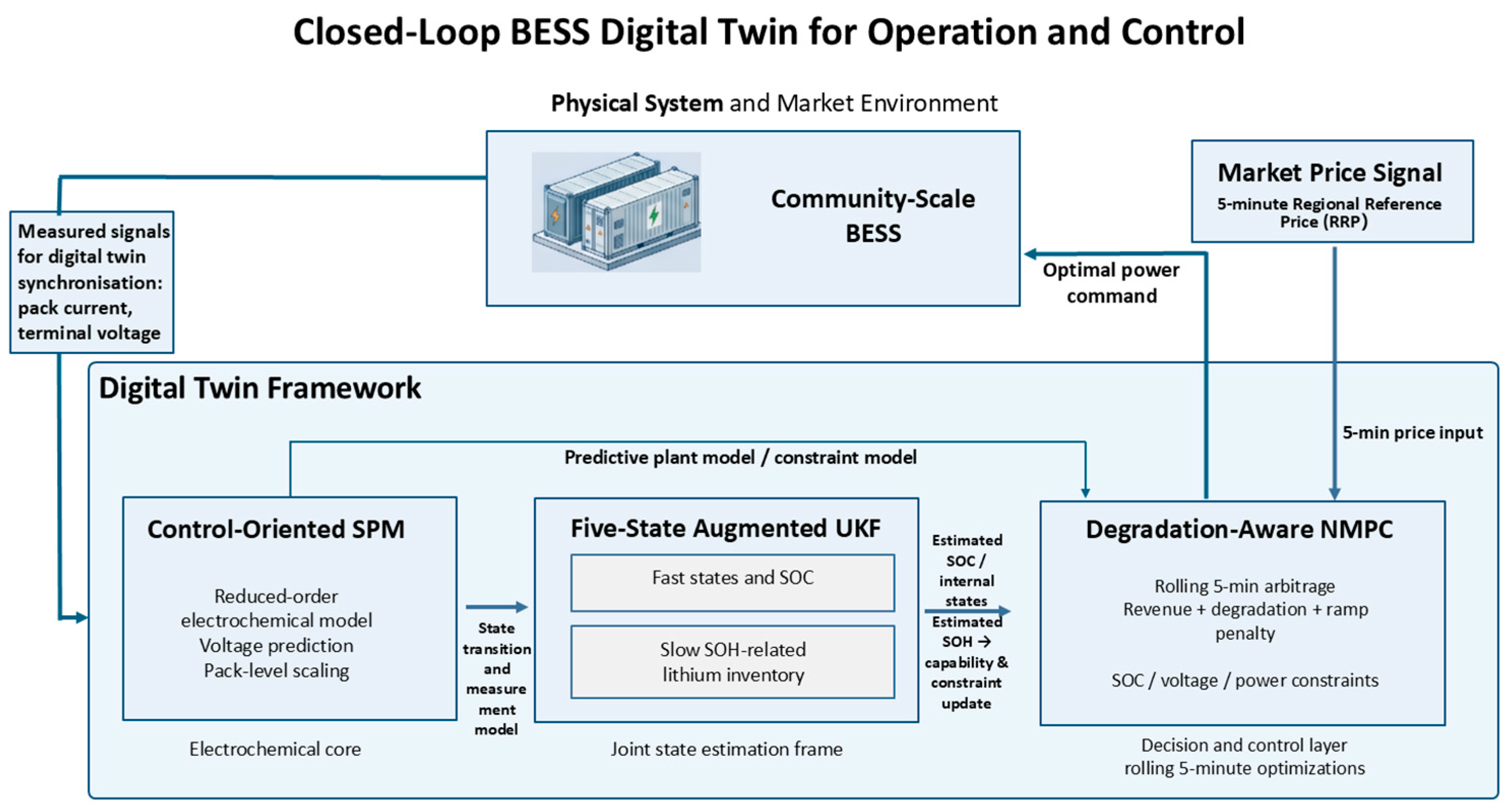
Before analysing the dispatch results, the performance of the UKF-based state estimation is first examined. In the proposed framework, the UKF updates the internal SPM states using terminal voltage measurements and provides SOC- and SOH-related information for the NMPC controller. The SOC result is used to evaluate the short-term tracking behaviour, while the SOH-related result is interpreted as a lithium-inventory-based health proxy rather than an independently validated ageing measurement. The following analysis presents the SOC tracking performance and SOH-oriented state evolution under dynamic charge–discharge operation.

3.1.1. SPM Parameterisation and Model Configuration

Table 1. SPM parameters.

Symbol	Anode	Cathode	Unit
$c_{s,i}^{\mathrm{m}\mathrm{a}\mathrm{x}}$	31,370	22,806	mol/m3
Ri	1.6192 × 10−5	9.7183 × 10−6	m
Si	11	22.3	m2
Ds,i	5.3125 × 10−14	1 × 10−14	m2/s
$c_{s,i}^0$	12,548	15,964	mol/m3
ki	9.9964 × 10−9	1.2496 × 10−11	m2.5 mol−0.5 s−1
R	8.3143		J mol−1 K−1
F	96,487		C/mol
T	298		K
c	1000		mol/m3

summarises the key parameters used in the control-oriented SPM adopted in this study. These parameters define the electrochemical characteristics of the battery cell and its aggregation into a 1 MW/4 MWh community-scale battery energy storage system.

The symbols denote maximum solid concentration $c_{s,i}^{\mathrm{m}\mathrm{a}\mathrm{x}}$, particle radius $R_i$, active surface area $S_i$, solid diffusion coefficient $D_{s,i}$, initial solid concentration $c_{s,i}^0$, reaction-rate constant k_i, gas constant R, Faraday constant F, temperature T, and electrolyte concentration c.

In addition to the SPM parameters listed in Table 1, the UKF configuration is specified to improve the reproducibility of the state-estimation results. The estimator uses a five-dimensional augmented-state vector, including four reduced electrochemical states and one lithium-inventory-related state. The terminal voltage is used as the measurement output, and additive voltage measurement noise is assumed. The main UKF covariance and noise settings are summarised in

Table 2. UKF configuration used in the state estimation simulation.

Item	Setting
State vector	${\left[{\overline{c}}_n,{\overline{q}}_n,{\overline{c}}_p,{\overline{q}}_p,n_{\mathrm{L}\mathrm{i}}\right]}^T$
Initial lithium inventory	$n_{\mathrm{L}\mathrm{i},0}=0.4c_{s,n}^{\mathrm{m}\mathrm{a}\mathrm{x}}{S}_n$
Measurement output	Terminal voltage
Measurement model	$V=h\left(x_{1:4},u\right)$
Additive measurement noise	Yes
Initial covariance P0	$diag\left[{\left(0.01c_{s,n}^{\mathrm{m}\mathrm{a}\mathrm{x}}\right)}^2,{\left(0.02\right)}^2,{\left(0.08c_{s,p}^{\mathrm{m}\mathrm{a}\mathrm{x}}\right)}^2,{\left(0.02\right)}^2,{\left(0.1n_{\mathrm{L}\mathrm{i},0}\right)}^2\right]$
Process noise Q	$diag\left[{\left(10^{-5}{c}_{s,n}^{\mathrm{m}\mathrm{a}\mathrm{x}}\right)}^2,{\left(10^{-6}\right)}^2,{\left(10^{-5}{c}_{s,p}^{\mathrm{m}\mathrm{a}\mathrm{x}}\right)}^2,{\left(10^{-6}\right)}^2,{\left(10^{-4}{n}_{\mathrm{L}\mathrm{i},0}\right)}^2\right]$
Measurement noise R	$(5\times 10^{-3}{)}^2{\mathrm{V}}^2$
Sampling time	300 s
Sigma-point parameters	MATLAB default values

.

The battery cell considered here is a 35.4 Ah LFP/graphite cell operating at 25 °C, with a nominal voltage of about 3.2 V. Fixed electrochemical parameters are kept constant, whereas lithium-inventory- and capacity-related variables are updated online through the UKF framework. In particular, those variables related to lithium inventory and effective capacity are allowed to vary slowly over time, so that the model can reflect the gradual degradation that occurs during operation.

3.1.2. State-of-Charge (SOC) Estimation Results

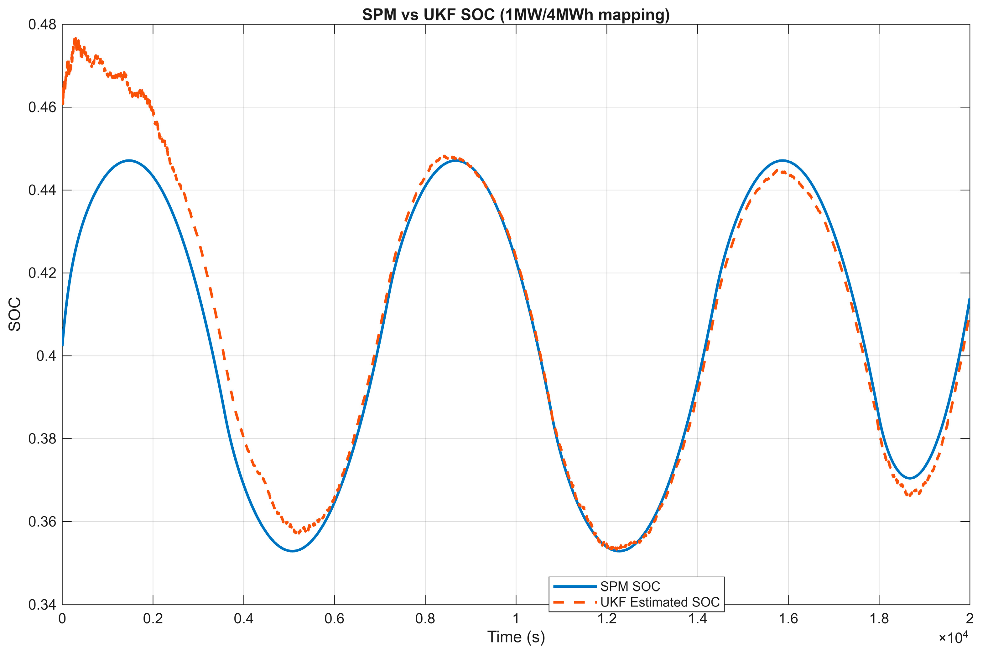
Figure 2 compares the UKF-estimated SOC with the simulated SPM reference SOC under the dynamic charge–discharge profile. The estimated SOC follows the main variation trend of the reference trajectory over the simulation period. A small deviation can be observed during transient changes, but the estimator remains stable and does not show divergence.

The SOC estimation error is further quantified using the root mean square error (RMSE). The obtained SOC RMSE is 0.0114 in absolute fraction, corresponding to approximately 1.14%. This result indicates that the UKF provides a reasonable SOC estimate for the subsequent NMPC dispatch calculation under the tested simulation condition.

It should be noted that the reference SOC is generated from the SPM-based simulation environment. Therefore, this comparison is interpreted as a model-based consistency check rather than an experimental validation using measured battery ageing data.

3.1.3. State-of-Health (SOH) Estimation Results

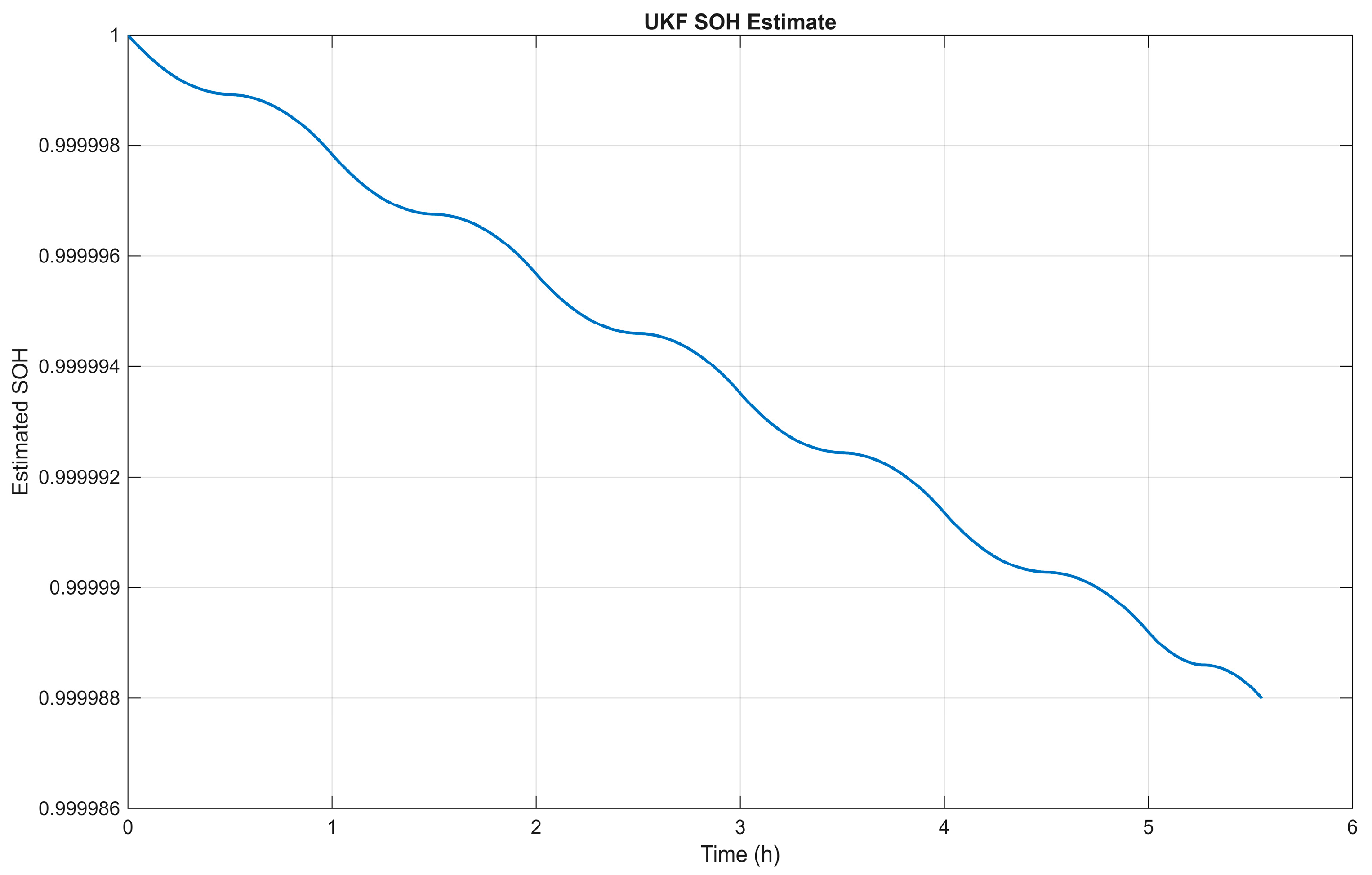
Figure 3 presents the evolution of the SOH-related state during the same dynamic operating condition. In this study, the SOH result is derived from the lithium-inventory-related state in the augmented SPM–UKF framework. Therefore, it should be interpreted as a model-consistent health-state proxy rather than an independently validated measurement of battery ageing.

The SOH-related trajectory changes gradually over the simulated operating period, which is consistent with the slow timescale of battery degradation compared with SOC dynamics. Unlike the SOC, which responds directly to charge and discharge current, the SOH-oriented state mainly reflects the accumulated effect of battery utilisation within the simplified degradation representation. The smooth evolution of this state suggests that the estimator can provide a stable internal health indicator for the degradation-aware NMPC controller.

However, because the simulation window is relatively short and no external ageing dataset is used for validation, the SOH result is not intended to demonstrate absolute ageing estimation accuracy. Instead, it is used to support the closed-loop control framework by providing a consistent internal health-state signal for comparing different dispatch strategies. Therefore, the quantitative assessment of degradation exposure in this study is mainly based on throughput, EFC, and degradation cost reported in

Table 3. Economic and battery utilisation metrics for the four regional 8 h NMPC cases.

Region	NSW (1 January 2025)	QLD (26 January 2023)	SA (8 December 2023)	VIC (15 August 2023)
Energy cashflow (A$)	659.74	661.40	6593.95	3641.84
Degradation cost (A$)	230.16	180.21	216.29	238.04
Ramp cost (A$)	3.72	14.39	17.44	19.53
Terminal penalty (A$)	26.17	29.14	94.48	57.66
Net profit (A$)	399.70	437.65	6265.75	3326.61
Throughput (kWh)	9206.3	7208.6	8651.6	9521.7
EFC	1.18	0.92	1.11	1.22
Final SOC, ${\theta }_n$	0.5911	0.6077	0.6009	0.6069

,

Table 4. Economic and battery utilisation comparison under 4 h and 8 h prediction horizons.

Region	Horizon	Energy Cashflow (A$)	Degradation Cost (A$)	Net Profit (A$)	Throughput (kWh)	EFC	Final SOC, ${\mathsf{\theta }}_{\mathbf{n}}$
NSW	4 h	623.45	206.65	387.01	8266.0	1.06	0.5913
	8 h	659.74	230.16	399.70	9206.3	1.18	0.5911
QLD	4 h	721.30	182.74	493.14	7309.8	0.93	0.6077
	8 h	661.40	180.21	437.65	7208.6	0.92	0.6077
SA	4 h	6628.97	218.81	6294.18	8752.3	1.12	0.5991
	8 h	6593.95	216.29	6265.75	8651.6	1.11	0.6009
VIC	4 h	3778.92	293.43	3407.03	11,737.1	1.50	0.6070
	8 h	3641.84	238.04	3326.61	9521.7	1.22	0.6069

and

Table 5. Sensitivity of 4 h NMPC results to the degradation-penalty weight.

Region	Case	Energy Cashflow (A$)	Degradation Penalty (A$)	Net Value (A$)	Throughput (kWh)	EFC	Final SOC, θn
NSW	${\mathsf{\lambda }}_{\mathrm{d}\mathrm{e}\mathrm{g}}$ = 0.025	623.45	206.65	387.01	8266.0	1.06	0.5913
	${\mathsf{\lambda }}_{\mathrm{d}\mathrm{e}\mathrm{g}}$ = 0	612.94	0	596.74	9728.7	1.24	0.6340
QLD	${\mathsf{\lambda }}_{\mathrm{d}\mathrm{e}\mathrm{g}}$ = 0.025	721.30	182.74	493.14	7309.8	0.93	0.6077
	${\mathsf{\lambda }}_{\mathrm{d}\mathrm{e}\mathrm{g}}$ = 0	640.40	0	599.59	12,002.6	1.53	0.6289
SA	${\mathsf{\lambda }}_{\mathrm{d}\mathrm{e}\mathrm{g}}$ = 0.025	6628.97	218.81	6294.18	8752.3	1.12	0.5991
	${\mathsf{\lambda }}_{\mathrm{d}\mathrm{e}\mathrm{g}}$ = 0	6656.04	0	6545.16	15,872.6	2.03	0.6023
VIC	${\mathsf{\lambda }}_{\mathrm{d}\mathrm{e}\mathrm{g}}$ = 0.025	3778.92	293.43	3407.03	11,737.1	1.50	0.6070
	${\mathsf{\lambda }}_{\mathrm{d}\mathrm{e}\mathrm{g}}$ = 0	3695.37	0	3626.20	13,169.3	1.68	0.6288

, while the SOH trajectory is used as a model-consistent internal health indicator.

3.2. Economic Dispatch Results Based on NMPC

We use the UKF-based state estimation results to evaluate the economic dispatch performance under the NMPC framework, where the estimated SOC and SOH are fed into the controller to determine the charging and discharging actions.

The analysis is organised into seven parts: (i) intraday dispatch behaviour in NSW under an 8 h horizon, (ii) cross-regional comparison, (iii) the impact of prediction horizon length, (iv) degradation-penalty sensitivity, (v) forecast-error sensitivity, (vi) comparison with a rule-based baseline strategy, and (vii) computational performance under the five-minute dispatch interval.

It should be noted that the price inputs used in this study are historical five-minute NEM RRP data rather than forecasted prices. Therefore, the dispatch results are interpreted as a perfect-foresight simulation benchmark for evaluating the proposed control framework, rather than as a fully forecast-driven real-time operation result. In this sense, the reported arbitrage values should be regarded as an upper-bound assessment of the proposed NMPC structure under the selected price profiles.

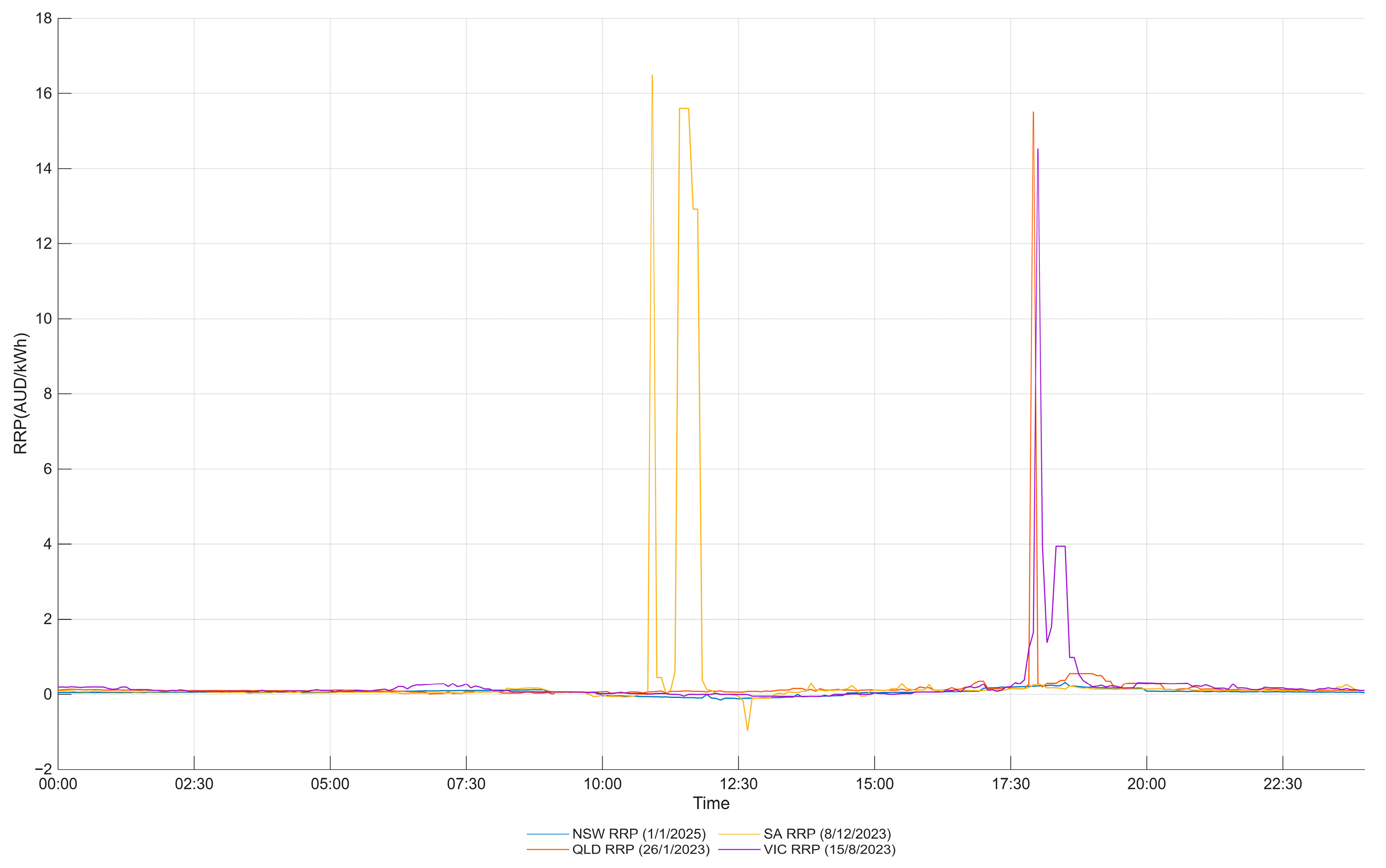
Figure 4 shows the electricity price curves for the selected representative day in the four states. Price variation in NSW is relatively smooth, whereas the other three states exhibit extreme price spikes. VIC, for example, includes not only extreme events but also sustained high-price periods at the level of several thousand dollars, which create a strong incentive for arbitrage. Negative electricity prices occur in both the NSW and SA markets. The presence of these differences allows our analysis to cover a range of different market conditions.

3.2.1. Intraday Dispatch Behaviour in NSW Under an 8 h Prediction Horizon

The NSW case is simulated for 24 h using five-minute settlement data. At each time step, the UKF-based digital twin provides an estimated augmented state for NMPC initialization, and this state includes the fast-varying state variables related to the SOC as well as the SOH. Then, NMPC solves the nonlinear optimisation problem over an eight-hour prediction horizon in order to determine the final control action.

The objective maximises arbitrage value while regularising degradation and control smoothness: a throughput-based degradation penalty with ${\lambda }_{\mathrm{d}\mathrm{e}\mathrm{g}}=0.025\mathrm{A}\mathrm{U}\mathrm{D}/\mathrm{k}\mathrm{W}\mathrm{h}$ and a ramp penalty with ${\lambda }_{\mathsf{\Delta }u}=0.01\mathrm{A}\mathrm{U}\mathrm{D}/{\mathrm{A}}^2.$ A terminal SOC soft constraint is enabled to steer the negative-electrode SOC toward ${\theta }_{n,\mathrm{r}\mathrm{e}\mathrm{f}}=0.7$, with an adaptive terminal weight scaled by the maximum |price| within the prediction window. Operational constraints include electrode SOC bounds [0.03, 0.97], cell-voltage limits (2.70–4.20 V), and a pack power limit. SOH feedback is enabled such that the effective energy capacity and power limit are scaled proportionally with the SOH, reflecting degradation-aware operational capability.

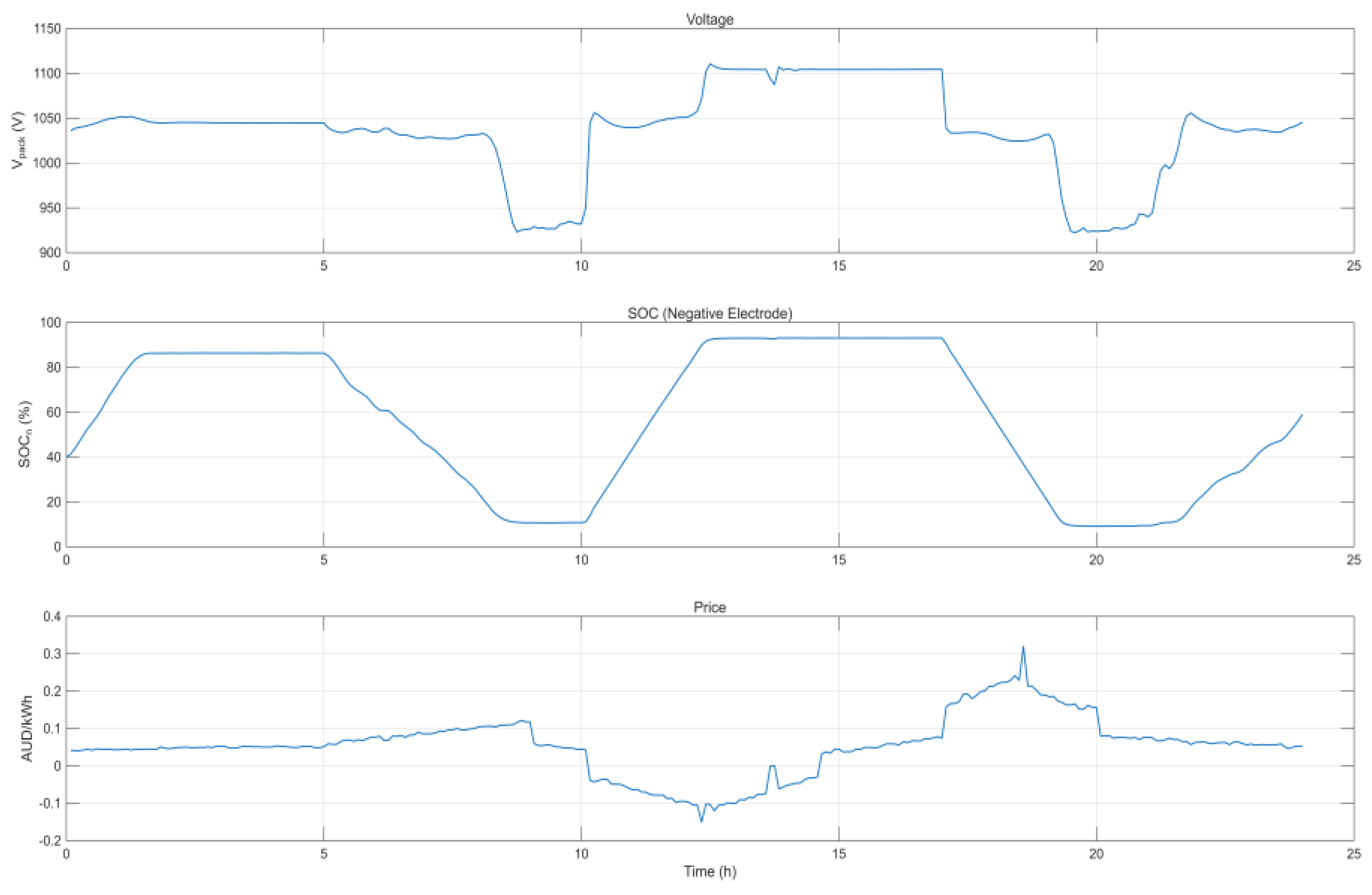
Figure 5 presents the electricity price, battery voltage, and SOC trajectories for the NSW case under the 8 h prediction horizon. Overall, the SOC variation is broadly consistent with the arbitrage logic of charging during low-price periods and discharging during higher-price periods. In the early hours, the electricity price remains positive and changes only moderately. The SOC first stays at a relatively high level and then decreases between approximately 5 h and 9 h, indicating that the battery releases energy when the price is still favourable compared with the later low-price period.

A more obvious charging response occurs around the middle of the day. When the electricity price drops to a low or negative level, the SOC increases rapidly from a low value to a high value. This indicates that the controller charges the battery when electricity is economically favourable. Such behaviour is consistent with the purpose of price arbitrage, because storing energy during negative- or low-price intervals can create value for later discharge.

Later in the day, the electricity price rises again and reaches a higher level in the evening. During this period, the SOC decreases sharply, showing that the stored energy is discharged during the high-price interval. Therefore, the NSW result generally follows the expected economic dispatch pattern of charging at low prices and discharging at high prices. At the same time, the SOC trajectory also shows that the controller does not respond only to the current price. Instead, it considers the price distribution over the 8 h prediction horizon, together with SOC constraints, voltage limits, degradation-related cost, and the terminal SOC requirement.

3.2.2. Cross-Regional Comparison Under an 8 h Prediction Horizon

Table 3 summarises the economic and battery utilisation metrics for the four regional cases under the 8 h prediction horizon. The results show clear regional differences in arbitrage performance. Among the four regions, SA achieves the highest net profit, reaching A$6265.75. This is mainly due to its much larger energy cashflow of A$6593.95, which reflects the presence of strong price spreads within the selected day. VIC also shows a high net profit of A$3326.61, indicating that its price profile provides substantial arbitrage opportunities, although the total revenue is lower than that of SA.

In contrast, NSW and QLD show much lower net profits, with A$399.70 and A$437.65, respectively. Their energy cashflows are also close, both around A$660. However, QLD obtains a slightly higher net profit than NSW because its degradation cost is lower. This suggests that similar revenue levels can lead to different final profits once battery utilisation and degradation-related cost are considered.

The battery utilisation metrics further show that higher profit does not depend only on the maximum electricity price. VIC has the highest throughput and EFC, reaching 9521.7 kWh and 1.22 EFC, respectively. This indicates more intensive battery cycling and also explains why VIC has the highest degradation cost among the four cases. SA, although having the highest net profit, does not have the highest throughput or degradation cost. This implies that its profit is mainly driven by more favourable price spreads rather than simply by heavier battery usage.

Overall, the cross-regional comparison demonstrates the trade-off between arbitrage revenue and battery wear. Regions with larger price spreads can generate higher energy cashflow, but the final profit is also affected by degradation cost, ramping cost, terminal penalty, and the amount of battery throughput. Therefore, the dispatch performance cannot be explained by electricity price peaks alone. It depends on how profitable price events are distributed over time and how much battery utilisation is required to capture them.

3.2.3. Comparison Between 4 h and 8 h Prediction Horizons Across Regions

Table 4 shows that increasing the prediction horizon from 4 h to 8 h does not consistently improve the daily net profit. In NSW, the 8 h horizon gives a slightly higher net profit, increasing from A$387.01 to A$399.70. However, this improvement is obtained with higher throughput and degradation cost, indicating that the additional profit comes with more intensive battery use. In QLD, SA, and VIC, the 8 h horizon reduces the degradation cost, but the penalised net profit is also slightly lower than that of the 4 h case. This suggests that a longer horizon changes the trade-off between arbitrage revenue and battery utilisation, rather than simply improving all performance indicators.

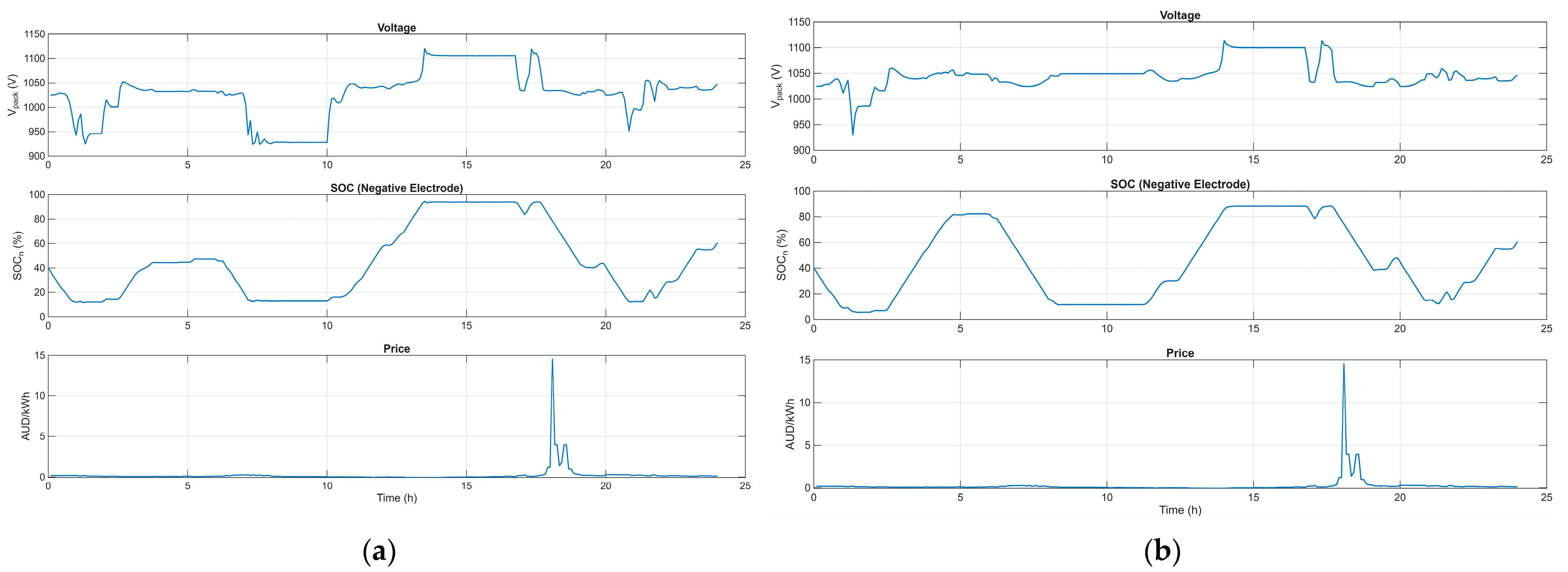
Figure 6 further illustrates the difference between the two horizons using the VIC case, where the change in SOC behaviour is more visible. Under the 4 h horizon, the SOC changes more actively in response to short-term price variations, which leads to higher throughput and a higher EFC. This is consistent with the numerical results in Table 4, where the 4 h case reaches 11,737.1 kWh throughput and 1.50 EFC. Under the 8 h horizon, the SOC trajectory is less aggressive, and the battery is used more conservatively over the same price profile. As a result, the throughput decreases to 9521.7 kWh and the EFC decreases to 1.22.

In the VIC case, the 4 h horizon achieves a slightly higher net profit of A$3407.03, while the 8 h horizon gives A$3326.61. However, the 8 h horizon reduces the degradation cost from A$293.43 to A$238.04. Therefore, the 8 h horizon does not maximise the one-day profit in this case, but it reduces battery cycling intensity and degradation-related cost. This comparison indicates that the prediction horizon affects not only the economic return, but also how intensively the battery is used. The horizon length should therefore be understood as a trade-off between short-term arbitrage revenue and degradation-aware operation, rather than as a parameter that is always better when made longer.

3.2.4. Degradation-Penalty Sensitivity Analysis

To examine the influence of the degradation penalty in the NMPC objective, an additional sensitivity case is conducted by setting ${\mathsf{\lambda }}_{\mathrm{d}\mathrm{e}\mathrm{g}}$ = 0. In the original degradation-aware case, ${\mathsf{\lambda }}_{\mathrm{d}\mathrm{e}\mathrm{g}}$ is set to 0.025 A$/kWh. The comparison is performed under the 4 h prediction horizon for all four regions. The ${\mathsf{\lambda }}_{\mathrm{d}\mathrm{e}\mathrm{g}}$ = 0 case removes the degradation penalty from the optimisation objective, so the controller becomes more focused on short-term arbitrage revenue. Therefore, this case serves as a degradation-agnostic NMPC ablation for evaluating the behavioural effect of the degradation-aware term.

Table 5 shows that removing the degradation penalty generally increases battery utilisation. In all four regions, the ${\mathsf{\lambda }}_{\mathrm{d}\mathrm{e}\mathrm{g}} = 0$ case produces higher throughput and EFC than the original degradation-aware case. This effect is especially clear in QLD and SA, where EFC increases from 0.93 to 1.53 and from 1.12 to 2.03, respectively. This indicates that, without the degradation penalty, the controller is more willing to use the battery intensively to capture price differences.

The change in energy cashflow is not uniform across regions. In SA, removing the degradation penalty slightly increases the energy cashflow, while in NSW, QLD, and VIC it does not. This suggests that higher cycling does not always lead to higher arbitrage revenue. Some additional charge–discharge actions increase throughput but do not necessarily provide sufficient economic benefit.

The reported net value of the ${\mathsf{\lambda }}_{\mathrm{d}\mathrm{e}\mathrm{g}} = 0$ case is higher because the degradation penalty is excluded from the objective. Therefore, it should not be interpreted as a degradation-inclusive profit. The main purpose of this comparison is to show how the degradation penalty changes the dispatch behaviour. Overall, the results confirm that including ${\mathsf{\lambda }}_{\mathrm{d}\mathrm{e}\mathrm{g}}$ helps limit unnecessary battery cycling and supports a more degradation-aware operating strategy.

3.2.5. Forecast-Error Sensitivity Analysis

The previous dispatch results are based on a perfect-foresight price benchmark, where the historical RRP trajectory is used inside the NMPC prediction horizon. To examine the effect of imperfect price information, a forecast-error sensitivity test is further conducted under the 4 h prediction horizon. In this test, uniform random errors of ±5% and ±10% are added only to the predicted future prices used by the NMPC. The realised economic performance is still evaluated using the original historical RRP data. Forecast errors were introduced as multiplicative uniform perturbations to the future prices used inside the NMPC prediction horizon. Specifically, ${\widehat{\pi }}_{k+j}={\pi }_{k+j}(1+{ϵ}_{k+j})$, where ${\pi }_{k+j}~U(-r,r)$, with $r$ = 0.05 or 0.10. The current dispatch price was not perturbed, and the realised economic performance was evaluated using the original historical RRP. A fixed random seed was used for reproducibility, so

Table 6. Forecast-error sensitivity results under the 4 h prediction horizon.

Region	Forecast Case	Net Profit (A$)	Change vs. Perfect (%)	Energy Cashflow (A$)	Degradation Cost (A$)	Throughput (kWh)	EFC	Final SOC, θn
NSW	$\mathrm{P}\mathrm{e}\mathrm{r}\mathrm{f}\mathrm{e}\mathrm{c}\mathrm{t}$	387.01	–	623.45	206.65	8266.0	1.06	0.5913
	±5% error	449.64	+16.18	692.24	214.15	8566.1	1.10	0.5934
	±10% error	457.21	+18.14	690.63	206.08	8243.3	1.05	0.5954
QLD	$\mathrm{P}\mathrm{e}\mathrm{r}\mathrm{f}\mathrm{e}\mathrm{c}\mathrm{t}$	493.14	–	721.30	182.74	7309.8	0.93	0.6077
	±5% error	453.47	−8.04	681.61	184.06	7362.5	0.94	0.6102
	±10% error	465.10	−5.69	697.78	189.40	7575.8	0.97	0.6124
SA	$\mathrm{P}\mathrm{e}\mathrm{r}\mathrm{f}\mathrm{e}\mathrm{c}\mathrm{t}$	6294.18	–	6628.97	218.81	8752.3	1.12	0.5991
	±5% error	6298.05	+0.06	6629.44	219.23	8769.1	1.12	0.6013
	±10% error	6299.25	+0.08	6624.63	218.15	8725.8	1.12	0.6038
VIC	$\mathrm{P}\mathrm{e}\mathrm{r}\mathrm{f}\mathrm{e}\mathrm{c}\mathrm{t}$	3407.03	–	3778.92	293.43	11,737.1	1.50	0.6070
	±5% error	3403.46	−0.10	3721.84	245.29	9811.6	1.25	0.6094
	±10% error	3405.52	−0.04	3721.39	244.64	9785.6	1.25	0.6115

reports one reproducible random realisation rather than a Monte Carlo average. Therefore, this test does not represent a new electricity price scenario, but a robustness check of the controller under imperfect price forecasts.

The percentage change in net profit is calculated relative to the perfect-foresight case as:

$${\mathsf{\Delta }}_{\mathrm{p}\mathrm{r}\mathrm{o}\mathrm{f}\mathrm{i}\mathrm{t}}(\%)={\displaystyle \frac{J_{\mathrm{e}\mathrm{r}\mathrm{r}\mathrm{o}\mathrm{r}}-J_{\mathrm{p}\mathrm{e}\mathrm{r}\mathrm{f}\mathrm{e}\mathrm{c}\mathrm{t}}}{J_{\mathrm{p}\mathrm{e}\mathrm{r}\mathrm{f}\mathrm{e}\mathrm{c}\mathrm{t}}}}\times 100\%$$

where $J_{\mathrm{p}\mathrm{e}\mathrm{r}\mathrm{f}\mathrm{e}\mathrm{c}\mathrm{t}}$ is the net profit obtained using the original historical RRP trajectory in the prediction horizon, and $J_{\mathrm{e}\mathrm{r}\mathrm{r}\mathrm{o}\mathrm{r}}$ is the net profit obtained when forecast errors are added to the predicted future prices.

Table 6 shows that the influence of forecast error is region-dependent. In NSW, the perturbed forecast cases lead to higher net profit than the perfect-foresight case. This does not mean that forecast errors are beneficial in general. Rather, it shows that the random perturbation can slightly change the timing of charge and discharge actions, and in this particular daily profile the resulting schedule gives a higher realised value.

In QLD, the forecast-error cases reduce the net profit by about 5.69% to 8.04%. This suggests that the QLD case is more sensitive to price prediction errors, likely because the value of dispatch is strongly affected by short-duration price events. In contrast, SA and VIC show very small changes in net profit. For SA, the variation is less than 0.1%, while for VIC it is also close to zero. This indicates that the dispatch results in these two cases are relatively stable under the tested ±5% and ±10% forecast perturbations.

The battery utilisation metrics also show that forecast errors can change the cycling pattern. For example, VIC has lower throughput and EFC under the perturbed forecasts than under the perfect case, while QLD shows a slight increase in throughput and EFC. Overall, the sensitivity test indicates that moderate forecast errors do not fundamentally change the main conclusions of the dispatch analysis.

3.2.6. Comparison with the Rule-Based Baseline Strategy

To provide a benchmark for the proposed NMPC strategy, a causal rolling-quantile rule-based baseline is used for comparison. Unlike the NMPC case, this baseline does not use the future price trajectory within a prediction horizon. At each five-minute step, it updates the charging and discharging thresholds using only the previously observed RRP values. After a two-hour warm-up period, the battery is charged when the current price is below the historical 25th percentile and discharged when the current price is above the historical 75th percentile. SOC reserve limits are also imposed to avoid over-charging or over-discharging. In the final four hours, a terminal recovery mode is applied to guide the SOC back towards the target value. The same degradation cost, ramping cost, and terminal penalty formulations are then used to evaluate both strategies.

Table 7. Comparison between the proposed NMPC and the rule-based baseline under the 8 h prediction horizon.

Region	Proposed NMPC Net Profit (A$)	Rule-Based Baseline Net Profit (A$)	Improvement (A$)	Relative Improvement (%)	NMPC Degradation Cost (A$)	Baseline Degradation Cost (A$)
NSW	399.70	427.43	−27.73	−6.49	230.16	280.45
QLD	437.65	−354.88	792.53	223.32	180.21	249.03
SA	6265.75	6078.89	186.86	3.07	216.29	390.99
VIC	3326.61	2810.54	516.07	18.36	238.04	253.81

compares the penalised net profit and degradation cost of the proposed NMPC and the rule-based baseline under the 8 h prediction horizon. The results show that the proposed NMPC achieves higher net profit than the baseline in QLD, SA, and VIC. The improvement is especially clear in QLD, where the baseline produces a negative net value, while the proposed NMPC achieves a positive net profit of A$437.65. In SA and VIC, the NMPC also improves the net profit by A$186.86 and A$516.07, respectively.

The NSW case shows a different result. The rule-based baseline obtains a slightly higher net profit than the NMPC, with A$427.43 compared with A$399.70. However, this higher return is accompanied by a larger degradation cost. The baseline degradation cost in NSW is A$280.45, while the NMPC degradation cost is A$230.16. Similar patterns can also be observed in the other regions, where the NMPC consistently results in a lower degradation cost than the baseline.

This comparison indicates that the proposed NMPC does not simply maximise short-term arbitrage revenue. Instead, it balances energy cashflow with degradation-related cost and other penalty terms. As a result, the NMPC can reduce battery wear in all four cases, while still improving or maintaining competitive net profit in most regions. The baseline comparison therefore supports the degradation-aware nature of the proposed dispatch strategy.

Since the NMPC uses the historical price trajectory within the prediction horizon as a perfect-foresight benchmark, this comparison should not be interpreted as a fully realistic real-time forecasting test. Rather, it quantifies the potential value of predictive optimisation compared with a simple causal rule-based strategy under the selected simulation setting.

3.2.7. Computational Performance Under the Five-Minute Dispatch Interval

To evaluate the computational performance of the proposed NMPC implementation, the solver time of each five-minute dispatch step is recorded.

Table 8. NMPC solver-time statistics and real-time feasibility under 4 h and 8 h prediction horizons.

Region	Horizon	Mean Solve Time (s)	Max Solve Time (s)	95th Percentile (s)	Failed/Unfinished NLP Steps
NSW	4 h	3.95	30.51	16.60	13/288
	8 h	18.74	128.10	92.81	63/288
QLD	4 h	4.70	21.32	14.70	0/288
	8 h	20.21	57.03	55.79	73/288
SA	4 h	4.45	34.90	15.82	3/288
	8 h	18.99	63.84	55.12	89/288
VIC	4 h	2.59	13.21	8.51	4/288
	8 h	16.04	57.49	50.79	33/288

summarises the mean, maximum, and 95th percentile solve times for the four regional cases under the 4 h and 8 h prediction horizons.

The results show that all tested cases complete each optimisation step within the five-minute dispatch interval of 300 s. For the 4 h horizon, the mean solve time remains below 5 s in all regions, and the maximum solve time is no more than 34.90 s. When the prediction horizon is extended to 8 h, the computational burden increases, with the mean solve time rising to about 16–20 s and the maximum solve time reaching 128.10 s in the NSW case. However, these values are still below the 300 s scheduling interval.

The increase in computation time is expected because the 8 h horizon contains more decision variables and constraints than the 4 h horizon. This indicates a clear trade-off between longer look-ahead capability and computational complexity. In addition to solver time, the closed-loop SOC, voltage, and power trajectories were checked against the imposed hard constraints, and no hard-constraint violations were observed in the reported simulation cases. Although the time requirement is satisfied in all cases, some optimisation steps are marked as failed or unfinished, especially under the 8 h horizon. Therefore, the results suggest that the current MATLAB implementation is time-compatible with five-minute dispatch in the tested simulations, but further solver tuning and convergence robustness improvement would be required before real-time field deployment.

4. Discussion

4.1. Interpretation of the Main Findings

The results demonstrate that the proposed digital-twin framework enables economically meaningful five-minute arbitrage while maintaining operational feasibility. Across the tested scenarios, the SPM–UKF–NMPC structure translated volatile price signals into physically admissible charge–discharge decisions, including low- or negative-price charging and high-price discharging.

Prediction-horizon length also affected dispatch quality. The 8 h horizon enabled more anticipative and, in some cases, smoother SOC trajectories. However, it did not consistently improve daily net profit across all regions, indicating a trade-off between look-ahead capability, cycling intensity, degradation cost, and solver convergence quality [10,36].

The results also show that the key factor affecting dispatch behaviour and final profit is not simply the price magnitude itself, but more importantly the shape of the regional electricity price curve. Differences in the timing, duration, and clustering of negative electricity prices and evening price peaks directly lead to different charge–discharge patterns across regions. The inclusion of degradation and ramping penalties suppresses overly aggressive cycling, indicating that profitability can be improved without treating battery health as a secondary consideration [12,35].

4.2. Comparison with Existing Studies

These findings are consistent with prior studies showing that physics-informed battery models and predictive control improve grid-connected storage operation. In particular, the results support the use of SPMs as a tractable electrochemical model and UKF-based estimators for nonlinear battery-state reconstruction [19,32,40]. The proposed framework extends these ideas to five-minute NEM arbitrage while maintaining feasible SOC trajectories and stable estimation behaviour.

Compared with prior work, the main contribution is the integration of the control-oriented SPM, joint SOC/SOH estimation, and degradation-aware NMPC within a unified five-minute community-BESS arbitrage setting, extending studies that treat modelling, estimation, and optimisation separately or under less volatile price conditions [11,20,27].

From a computational-dispatch perspective, this study is also complementary to recent convex reformulation methods for energy management. For instance, Liang et al. improved the tractability of hybrid AC/DC networked microgrid dispatch by convexifying bidirectional-converter modelling [16]. In contrast, the present work does not focus on converter-level AC/DC dispatch convexification, but on electrochemical-state-aware BESS operation through SPM-based modelling, UKF-based SOC/SOH estimation, and degradation-aware NMPC under five-minute NEM price signals.

At the same time, the results remain in line with the broader literature in showing that profitability depends strongly on price shape, forecast horizon, and operational constraints [13,35,41]. Therefore, the findings should be interpreted as evidence of practical integration and scenario-based usefulness rather than as a universal performance advantage over all existing BESS control methods.

4.3. Practical Implications for Community-Scale BESS Operation

The results have several practical implications for community-scale BESS operation. First, they suggest that short-interval market participation should not rely only on fixed charging thresholds or heuristic peak–valley rules, because such methods are less able to respond to rapid price reversals and negative-price events. Instead, operators benefit from a control framework that combines state estimation with predictive optimisation, so that charging and discharging decisions remain consistent with SOC, voltage, power, and degradation limits [7,13].

For the 1 MW/4 MWh case, a moderately longer prediction horizon improved SOC smoothness and terminal-SOC management while remaining within the five-minute timing limit in the tested simulations, although the higher number of unfinished NLP steps indicates that solver robustness must be improved before deployment. This supports deployment strategies that reduce myopic dispatch behaviour. With more detailed ageing models and network constraints, the framework could be extended from arbitrage to peak shaving, grid support, and multi-service coordination [11,26,42,43].

4.4. Field Implementation and Validation

Since the present study is simulation-based, direct field-trial results are not reported. To address practical deployment,

Table 9. Proposed staged implementation and validation plan for field deployment of the digital-twin BESS framework.

Stage	Validation Activity	Baseline/Stress Case	Exit Criteria	Corrective Action
Offline simulation	Run the SPM–UKF–NMPC framework using historical five-minute NEM price data.	Rule-based control baseline; perfect-forecast case; forecast-error case; ±10% perturbation in key SPM parameters, including solid-phase diffusion coefficients, reaction-rate constants, internal resistance, effective capacity, and OCV coefficients.	No SOC, voltage, or power-limit violations; solver success rate ≥ 95%; net profit remains positive under stress cases; terminal SOC deviation remains within the predefined tolerance band.	Re-tune NMPC weights, terminal penalty, solver tolerances, model parameters, or safety margins before moving to HIL validation.
Model calibration	Calibrate the control-oriented SPM using measured current, voltage, SOC, and temperature data.	Charge, discharge, and rest-period data from BMS logs.	Voltage and SOC tracking errors remain within acceptable engineering limits; estimated internal states remain physically bounded.	Re-identify SPM parameters, revise OCV fitting, or simplify the model before controller integration.
Hardware-in-the-loop validation	Test the controller using a real-time battery emulator or digital real-time simulator.	Extreme positive-price spikes; deep negative-price periods; high-SOC and low-SOC boundary cases; noisy current/voltage measurements; missing price data; communication delay; solver non-convergence.	95th-percentile computation time < 60 s; maximum computation time < 300 s; failed or unfinished NLP steps < 5%; solve-time coefficient of variation < 20%; no hard-constraint violations.	Keep the controller in HIL testing; revise warm start, horizon length, solver tolerances, constraint margins, or fallback rule-based control.
Pilot field deployment	Apply the NMPC command as a supervisory EMS-level signal under BMS/PCS protection.	Shadow-mode comparison or controlled A/B test against existing rule-based control using the same price and battery-state data.	NMPC provides positive incremental net value compared with rule-based control; no increase in safety-limit violations; BMS/PCS override events remain rare; measured power tracking error remains within the accepted tolerance.	Continue shadow-mode operation, reduce control aggressiveness, or revert to rule-based control until safe incremental benefit is verified.
Long-term monitoring	Evaluate the controller over several weeks or months of operation.	Seasonal price variation; renewable-generation variability; long-term throughput accumulation; repeated high-volatility days.	Economic benefit remains stable across operating periods; EFC and SOH-proxy trends remain consistent with expected ageing behaviour; controller availability remains high.	Update degradation parameters, recalibrate the SOH proxy, revise the market-operation strategy, or adjust maintenance thresholds.

outlines a staged field implementation and validation plan, including offline testing, model calibration, hardware-in-the-loop validation, pilot deployment, and long-term monitoring.

The listed exit criteria are proposed for future field validation and are not presented as completed experimental results in this study.

4.5. Limitations

Several limitations should be noted. First, the framework was evaluated through simulation using representative high-volatility NEM price profiles but has not yet been validated through hardware-in-the-loop testing or field deployment.

Second, the control-oriented SPM and the degradation representation simplify thermal behaviour and detailed ageing mechanisms. The lithium-inventory SOH state and throughput-based degradation penalty are used as control-oriented proxies for battery health awareness rather than as experimentally validated ageing models. They do not explicitly capture temperature-dependent SEI growth, lithium plating, depth-of-discharge-dependent cycle ageing, calendar ageing, or mechanical stress. In addition, because an electro-thermal model is not included, possible residual errors caused by temperature gradients or heat-generation-dependent diffusion changes are not quantified in this study. Therefore, the reported SOH trajectory and degradation cost should be interpreted as comparative indicators for dispatch evaluation, rather than absolute predictions of long-term battery ageing.

Third, the current NMPC focuses on price arbitrage and does not explicitly include feeder-level network constraints, local load uncertainty, ancillary services, or grid-forming inverter dynamics.

Finally, price trajectories are treated as external inputs using historical five-minute RRP data within the prediction horizon. Therefore, the dispatch results represent a perfect-foresight benchmark rather than a fully forecast-driven real-time implementation. Forecasting errors, price bias, and uncertainty propagation may reduce realised arbitrage value and change the timing of charge–discharge decisions. A limited forecast-error sensitivity test is included in Section 3.2.5 using ±5% and ±10% random perturbations under the 4 h horizon. However, this test is limited to deterministic random-error cases and does not replace a fully forecast-driven, robust, or stochastic NMPC implementation.

5. Conclusions and Future Work

5.1. Main Conclusions

This study developed a data-driven digital-twin framework for simulation-based real-time management of a community-scale grid-connected BESS under five-minute NEM price signals. By integrating a control-oriented SPM, a five-state augmented UKF for weakly coupled SOC/SOH estimation, and degradation-aware NMPC, the framework coordinated internal battery-state estimation, constraint-aware dispatch, and degradation-related cost consideration under representative high-volatility price scenarios. The horizon comparison showed that longer prediction horizons can produce smoother SOC trajectories and reduce cycling intensity in some cases, but they do not always improve daily net profit. The recorded solver times remained below the five-minute dispatch interval in the tested simulations, although unfinished NLP steps indicate that further solver tuning is required before field deployment. Overall, these results support the potential of integrating mechanistic modelling, online estimation, and predictive control for community-BESS operation in volatile electricity markets, while further validation under forecast uncertainty, electro-thermal effects, and hardware or field conditions remains necessary.

5.2. Future Work

Future work should extend the proposed digital-twin framework in four directions. First, price and load forecasting uncertainty should be incorporated into the control layer through robust or stochastic NMPC. Second, the battery model can be enriched by including electro-thermal dynamics and more detailed ageing mechanisms. Third, the control objective can be expanded from single-service arbitrage to multi-service operation, including peak shaving, frequency support, and grid-forming inverter coordination. Finally, learning-based or edge-assisted control methods may be explored to reduce online computational burden and improve scalability for distributed community-BESS operation [44,45].