A Template-Based Approach for Generating Modelica Models of Building Electrical Systems from Semantic Models

Abstract

Building electrical systems are becoming increasingly complex as designers evaluate AC, DC, and hybrid distribution architectures, integrate distributed energy resources, and maintain alignment with evolving performance and reliability goals. Existing design tools are typically limited, non-interoperable, and unable to support continuous modeling across design phases, resulting in fragmented workflows and significant manual effort. This paper presents a template-based workflow that automates the generation of high-fidelity Modelica simulation models of building electrical systems from semantic models. The workflow supports both basic safety analysis and the power-flow simulation of AC, DC, and hybrid system architectures. A Python-based middleware (RDF2EMO) was developed to automate data extraction, template instantiation, and parametric model generation, enabling rapid and consistent iteration through schematic design, design development, and construction documentation phases. Verification of the middleware automation (RDF2EMO) using a reference medium-sized office building demonstrates that the generated Modelica model is internally consistent with the Building Information Model. A case study demonstrates how the workflow supports design decisions, including system architecture selection, equipment sizing impacts and optimization, and reliability analysis.

1. Introduction

Building electrical systems—encompassing power distribution, resiliency sources (e.g., diesel/gas generators, energy storage), and diverse loads (e.g., HVAC, lighting, miscellaneous electric loads)—can be designed in many different architectures (e.g., AC, DC, hybrid AC/DC), each offering distinct advantages. AC systems dominate legacy infrastructure due to their direct compatibility with utility grids. DC systems excel in integrating energy storage/generation equipment and DC-native loads, such as LED lighting and miscellaneous electric loads (MELs), with fewer conversion losses [1,2,3]. Hybrid AC/DC architectures combine flexibility for mixed loads with energy storage integration but introduce design complexity. Therefore, designers face several critical design decisions, such as whether to convert DC power from energy storage to AC for distribution or connect it directly to DC loads, and at what level (device, panel, zone, or building) to perform said conversions. These choices significantly impact system energy cost, resiliency, and alignment with other design goals, necessitating robust modeling and simulation to evaluate options.

Traditional mechanical, electrical, and plumbing (MEP) workflows typically follow a sequential process: conceptual design, schematic design (SD), design development (DD), construction document (CD), and commissioning. At each phase, data is generated, modified, or transferred, often manually, across tools like Revit, EasyPower, and ETAP to make design decisions [4,5,6]. For example, during the SD phase, engineers define the initial system architecture and component specifications, which are later finalized in the DD or CD phase by performing additional analysis. However, these design workflows are fragmented, involving multiple stakeholders—architects, electrical engineers, contractors, and facility managers—who use disparate tools and data formats at each design phase. This fragmentation leads to loss of critical data such as component specifications, connectivity details, or operational parameters, thereby complicating iterative design, increasing errors, and delaying project timelines. For instance, designers and contractors might not share models even in the same tools for short circuit analysis and equipment specification (e.g., EasyPower) and may manually build separate models, risking inconsistencies.

Building Information Modeling (BIM) offers a structured, machine-readable representation of building systems [7]. Semantic models, derived from BIM, enhance interoperability by using the ASHRAE 223 ontology for data. Modelica, an equation-based modeling language, excels in simulating complex systems with high fidelity, supporting dynamic analyses of AC, DC, and hybrid electrical systems. This paper proposes an automated workflow with a template-based modeling methodology that generates Modelica models populated with components from the BEEAM library using semantic information derived from Revit models. By mapping semantic data to executable Modelica code, the method reduces manual effort, preserves data integrity, and supports iterative design, enabling designers to explore architecture trade-offs, optimize equipment sizing, and ensure compliance with fire safety requirements.

2. Background

2.1. Existing Tools for Electrical Systems Modeling and Analysis

Many existing tools are available for use by MEP firms for designing building electrical systems. Some of the most commonly used and novel tools are summarized in

Table 1. Existing tools used by MEP firms for designing electrical systems [5,6,8,9,10,11,12,13,14].

	ElectroBIM	EasyPower	ETAP	SKM	PSSE	PowerWorld	MATPOWER	OpenIPSL	BEEAM
Language	–	–	–	–	–	–	MATLAB	Modelica	Modelica
License type	Licensed	Licensed	Licensed	Licensed	Licensed	Licensed	Open source	Open source	Open source
Scope	Buildings	Buildings	Buildings, Grid	Buildings, Grid	Grid	Grid	Grid	Grid	Buildings
Architecture	AC	AC, DC, hybrid	AC, DC, hybrid	AC, DC, hybrid	AC	AC	AC, DC	AC	AC, DC, hybrid
Model development	Revit plugin	Proprietary software	Proprietary software	Proprietary software	Proprietary software	Proprietary software	MATLAB IDE	Modelica IDE	Modelica IDE
Use cases	Voltage drop, short circuit, arc flash, selective coordination	Simple power flow, short circuit, arc flash, selective coordination	AC and DC load flow, AC and DC short circuit	AC and DC load flow, AC and DC short circuit, fault analysis	Power flow, short circuit, dynamic/ transient stability	Power flow, optimal power flow, fault analysis, transient stability	AC and DC power flow, continuous and optimal power flow	Dynamic phasor time-domain power flow	Harmonic power flow
Developer	Design Master	EasyPower	ETAP	SKM	Siemens	Power World corp.	Cornell University	ALSETLab at RPI	NRL

. While most existing tools are focused on analyzing short circuits, voltage drops, arc flash, and selective coordination, some are capable of power flow analysis. Similarly, while most tools require models to be developed in an internal and proprietary environment, some tools support integration with other building design tools (e.g., BIM) or modeling and simulation environments (e.g., MATLAB, Modelica).

The generally limited scope and interoperability of these existing tools require designers to manually recreate building system models to perform analyses. This fragmented environment introduces inconsistencies, increases modeling effort, and limits the reuse of data across design phases.

2.2. Automated Model Generation

A critical component of an integrated design and analysis workflow is the ability to generate simulation models from a central data source and then rapidly iterate multiple experiments on them. Previous work has proposed the use of templates for the automated generation of Modelica models. Nytsch-Geusen et al. [15] proposed an approach where generic Modelica models for HVAC air-side systems are constructed with indexed instances for the various components using an external templating engine. This allows users to conveniently generate various configurations with the use of table data structures, which are simple text-based classes that include the information required to generate and configure a wide variety of simulation models supported by the template. Gautier et al. [16] improved upon it with a Modelica-based templating methodology. Nytsch-Geusen et al. [17] also proposed the use of Modelica simulation model generation from templates, with the input being an Industry Foundation Classes (IFC) BIM file. The input file is parsed via the use of IfcOpenShell library, and the information is used to automatically generate a building thermal model with the Code Templating Tool (CoTeTo), a Python library specifically designed for generating thermal zone models. Similarly, Andriamamonjy et al. [18] proposed the use of IFC models for the generation of Modelica models that incorporate both the building thermal zones and the air-handling systems. The models are generated using a novel Python package called Ifc2Modelica.

Previous work clearly demonstrates that template and vectorization methodologies can be suitable and highly adaptable approaches for model generation across multiple building engineering domains. However, existing work is mostly focused on the modeling of mechanical systems and thermal energy and does not support electrical systems (e.g., lighting, appliances, battery energy storage systems) and electrical energy. Furthermore, while some previously demonstrated workflows tout integration with Building Information Models and related data models (i.e., IFC), they do not necessarily extend to the operational domain. Notably, no existing work was found that demonstrates the use of the emerging ASHRAE 223 ontology for building systems and leverages its ability to model building systems with high fidelity, including low-level functions and connectivity details that impact real-world performance.

3. Proposed Workflow

The proposed workflow leverages BIM tools that are foundational to most new construction and major retrofit projects. It incorporates four existing tools and one newly developed tool. Revit is used to design electrical systems and capture equipment, connectivity, and control details (e.g., load ratings, breaker sizes, wire gauges, control zones). ElectroBIM enables one-line diagram generation and fire-safety-compliant voltage drop, fault, and arc-flash calculations within Revit. Power flow simulation is enabled by Modelica, an object-oriented language for modeling cyber-physical systems.

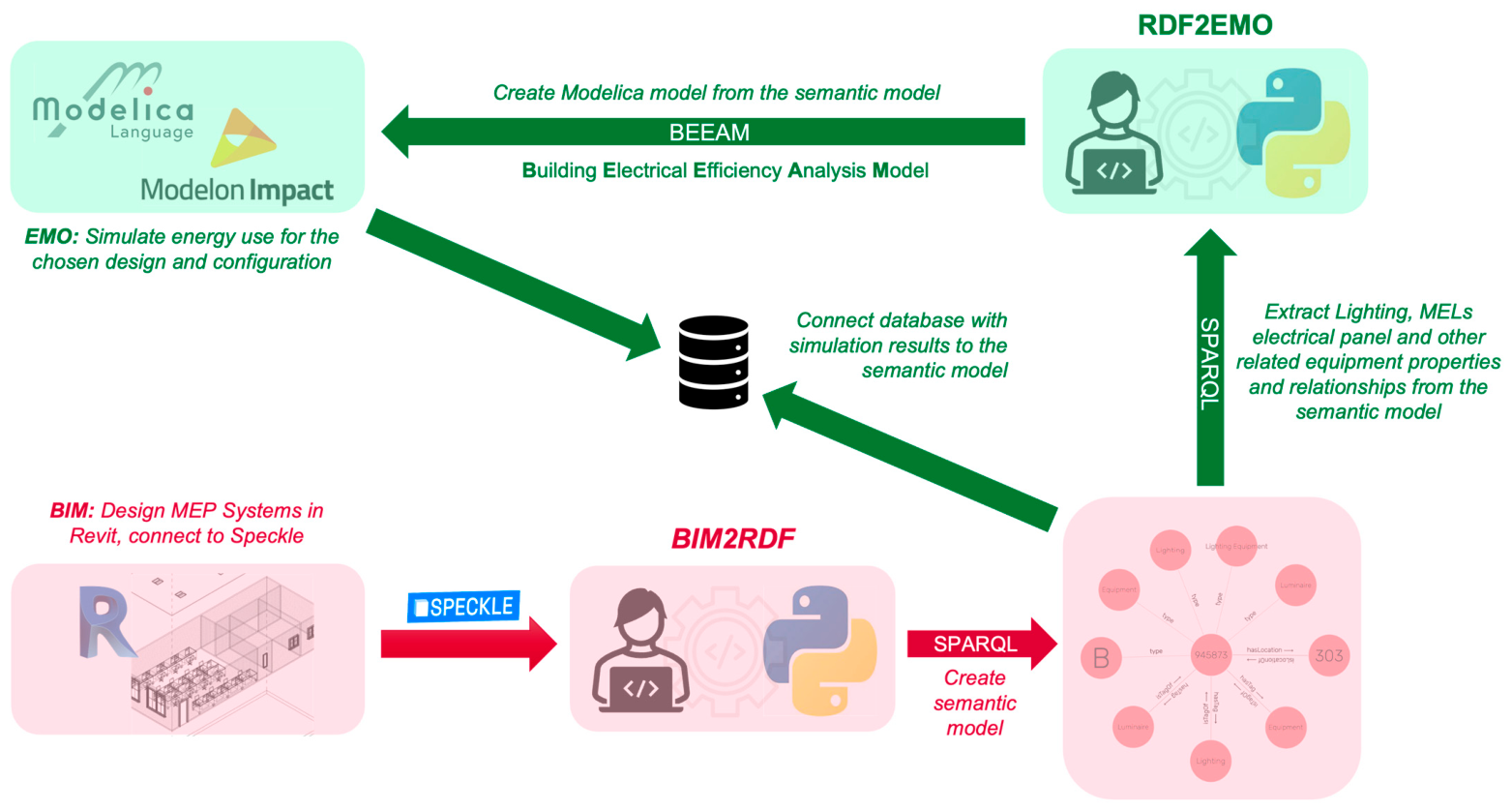
The tools and approach for generating Modelica models are summarized in Figure 1. BIM2RDF, a previously developed tool [19], is used to generate ASHRAE 223-compliant semantic models from the BIM through a Speckle interface [20]. Notably, the currently released version of BIM2RDF is limited to BIMs that can be connected to Speckle. A newly developed Python middleware tool (RDF2EMO) is used to create Modelica simulation models from the semantic model using the BEEAM Modelica library. BEEAM was previously verified and found to be capable of estimating power demand and energy use with an accuracy of ±5% [21,22,23]. The Modelica model is simulated in the Modelon Impact Integrated Development Environment (IDE) [24]. Modelica is an open-source language that in principle facilitates interoperability across IDEs. While the BEEAM library has been demonstrated to be compatible with other IDEs, including Dymola and OpenModelica, the results presented here are exclusively produced using Modelon Impact 4.113.0 [25,26,27]. Simulation results are connected back to the semantic model to provide the context necessary for analysis.

The workflow supports iterative design across the SD, DD, and CD phases. In SD, preliminary one-line diagrams and load estimates guide architecture selection. In DD and CD, detailed simulations refine equipment sizing and architecture selection and verify compliance with fire safety and utility requirements. The use of ASHRAE 223 to provide metadata context for the simulation results reduces the complexity and time required to configure digital twin applications that compare simulated and operational data. Notably, ASHRAE 223 leverages modern and powerful semantic web technologies that facilitate complex queries required by emerging approaches for automated control configuration, commissioning, fault detection and diagnostics, and performance management.

3.1. Automated Model Creation

Automated model creation is crucial for modeling whole building systems, which may include hundreds or even thousands of electrical devices on each floor. To address this challenge, three approaches were considered for developing the RDF2EMO Python tool that automates the creation of Modelica models.

3.1.1. Approach 1: Python Assembly Using Python Objects

In this approach, Python objects are created for each Modelica class, and a Python script assembles the entire model by instantiating the Python objects and populating their parameter values. This approach is simple to implement but can become complicated for large models. Python IDEs generally do not understand Modelica and thus cannot verify the Modelica code in the Python objects. As a result, models need to be loaded into a Modelica IDE to identify Modelica syntax errors, making verification a two-step process.

3.1.2. Approach 2: Python Assembly Using Model Templates

In this approach, model templates are created manually in the Modelica IDE. A Python script is used to assemble the entire model by instantiating these model templates and populating their parameter values. This approach is simple to implement, and the templates are inherently verified during their development in the Modelica IDE. Python scripts are only used to create the data record that instantiated the model templates. However, this approach requires the creation of a sufficient set of system model templates that support different electrical system architectures and connections.

3.1.3. Approach 3: Python Assembly Using Modelica IDE API Calls

In this approach, a Python script uses API calls to assemble the model by instantiating Modelica classes and populating their parameter values. As the entire model is created using an API, there is no need for complicated pre-built templates. However, this approach is very IDE dependent and requires that the Modelica IDE API has methods that can be used to make connections and configure parameters.

3.2. A Template-Based Approach to Automated Model Creation

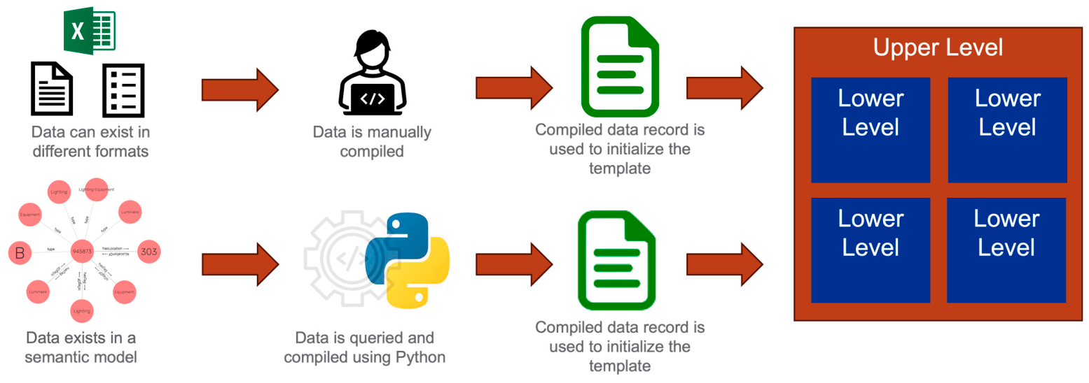
Approach 2 was selected for further development based on the compelling results delivered by previous work that used a similar approach for HVAC systems [15,16,17,18]. A whole-building electrical system is modeled as a two-level system such that the upper level defines the system architecture and the lower level defines the sub-systems (e.g., lighting and plug loads). These templates are instantiated using data records that can be created from data in a prescribed format or from querying a semantic model (Figure 2).

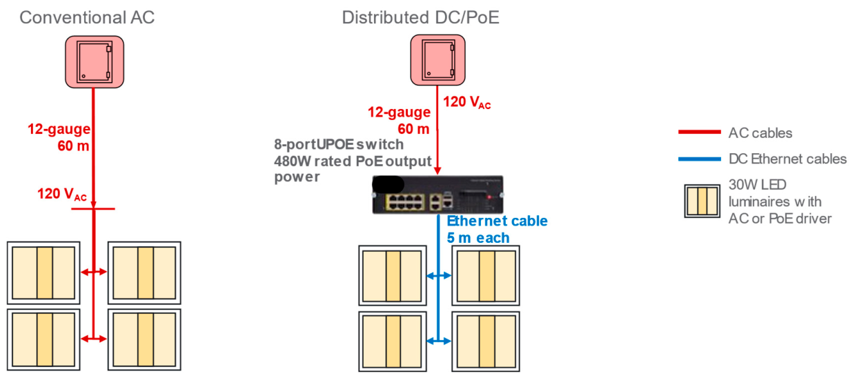
The two-level system was developed by considering two simple four-luminaire lighting systems, one powered by a conventional AC architecture and the other by a distributed DC/Power-over-Ethernet (PoE) architecture (Figure 3).

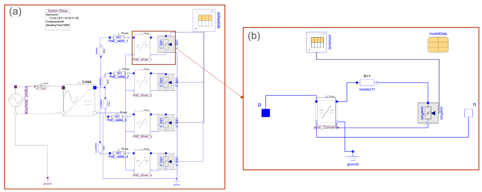
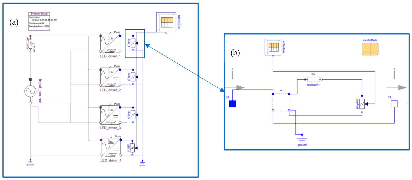
When the distributed DC/PoE system is modeled in Modelica, it mainly consists of an input source, an AC/DC converter (PoE switch), four DC/DC converters (PoE drivers), and four variable DC loads (LED modules), as shown in Figure 4a. As there are multiple instances of DC/DC converters and variable loads, a simple lower-level load template can be created from a distributed DC whole-system model, consisting of a DC/DC converter with a variable load (Figure 4b).

Similarly, when a conventional AC system is modeled in Modelica, it mainly consists of an input source, four AC/DC converters (AC LED drivers), and four variable loads, as shown in Figure 5a. This system does not have DC/DC converters. The same load template can be used in this case as well by making the DC/DC converter a replaceable component and setting it to an electrical “short” (Figure 5b).

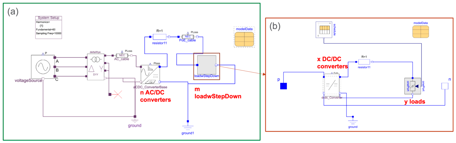
Using this common lower-level load template “loadwStepDown”, a simple upper-level template can be created that supports multiple system architectures (Figure 6a). The simple upper-level template consists of an input source (voltage source and transformer), vectorized AC/DC converters, and vectorized loadwStepDown. Each loadwStepDown consists of vectorized replaceable DC/DC converters and vectorized variable DC loads. This vectorization of components enables the user to expand the system model that consists of ‘n’ AC/DC converters, each with ‘m’ loadwStepDown (internally consisting of ‘x’ DC/DC converters, each with ‘y’ loads) and achieve multiple system architectures (Figure 6b).

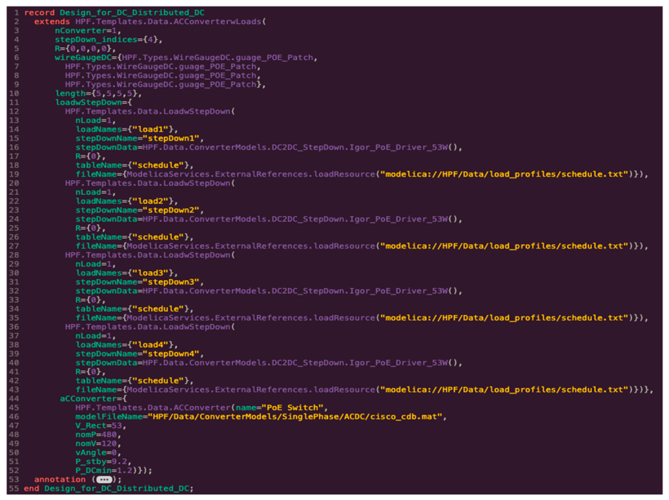
This template can be configured via a data record that is automatically generated from a user input file using a Python script. In Modelica, a data record can have variables, just like a model, but cannot include equations. Data records are primarily used to group data together. Model parameter values that correspond to different components in the template are given as input to the Python script. In this demonstration, the input is in the form of a JSON object read from a file. In the integrated workflow, the input will be directly generated by queries on the semantic model. Python functions are used to generate text blocks that assign parameter values for each converter type per the Modelica language data record syntax. All these blocks of text are combined into a Modelica data record that is used to instantiate the template (Figure 7).

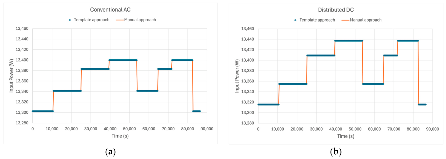
This template is verified by configuring it for the two four-luminaire lighting systems. The template is configured to represent a four-luminaire distributed DC/PoE system by setting n = 1, m = 4, and x = 1, y = 1 for each m. Similarly, the template is configured to represent a four-luminaire conventional AC system by setting n = 4, m = 1 for each n, and x = 1, y = 1 for each m. The template is simulated with data records for each of the two lighting systems, and the results are compared with the manually constructed model. The input power draw of the models constructed using the template and the manual approach matched in both conventional AC and distributed DC/PoE architectures (Figure 8). This shows that the template approach generates accurate models and can be used to build models for whole-building electrical systems.

4. Workflow Verification

Following the template-based method, whole-building lighting system models are created from a semantic model. An upper-level template is created that supports three high-fidelity implementations of a reference medium office model that was derived from one of the U.S. Department of Energy’s suite of commercial prototype building models [28]. The three electrical implementations have different system architectures: one that uses Conventional AC distribution, one that uses a hybrid of Conventional AC and Distributed PoE distribution, and one that uses a hybrid of Conventional AC and Centralized PoE distribution.

4.1. Conventional AC

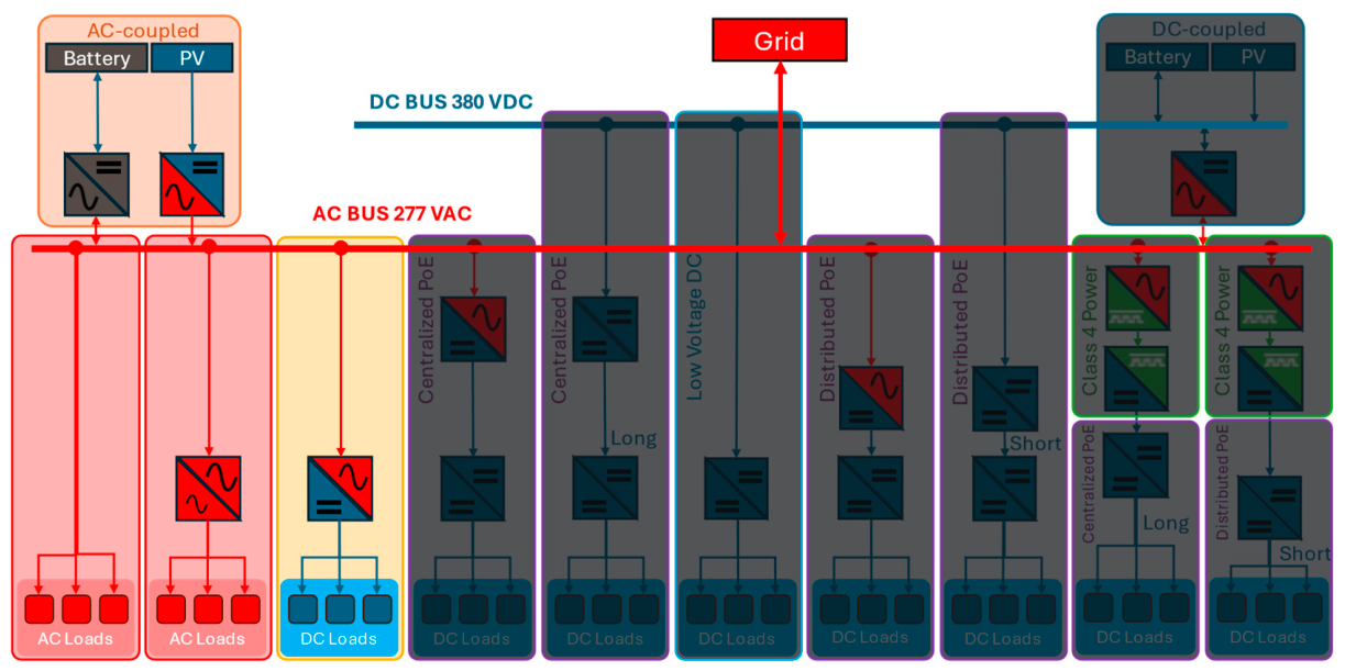
Conventional AC is the most common architecture found in buildings, where everything is coupled to the AC bus. PV is AC-coupled via an inverter, AC loads are directly coupled, and the DC loads are coupled via AC/DC converters at each load (Figure 9).

4.2. Distributed PoE

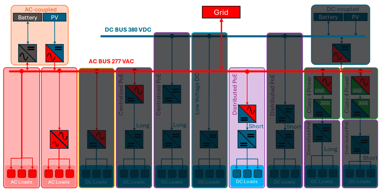
In the Distributed PoE architecture, PV is AC-coupled via an inverter and the AC loads are directly coupled to the AC bus. The DC loads are powered via a higher number of smaller PoE switches (AC/DC converters) distributed throughout the building, closer to the loads, and PoE drivers (DC/DC converters) at each load (Figure 10).

4.3. Centralized PoE

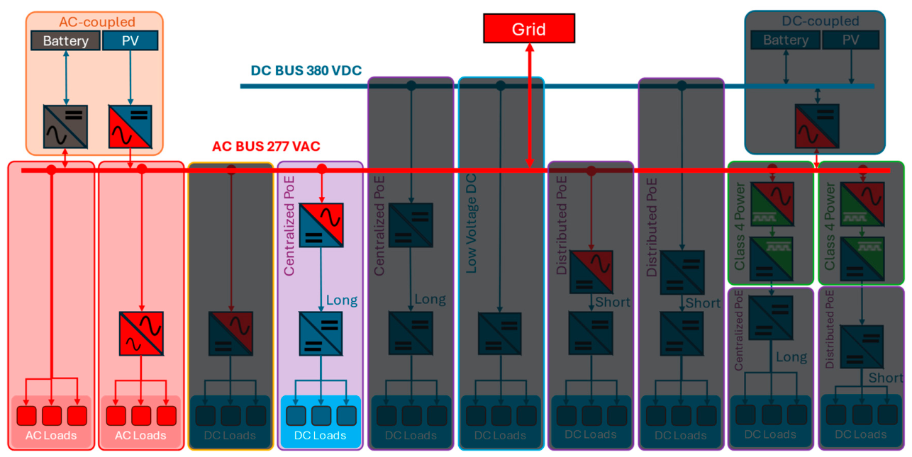
The Centralized PoE architecture is similar to the Distributed PoE architecture, except for the placement and type of PoE switches. In this architecture, bigger PoE switches capable of powering a higher number of loads are placed in a central location in the building. DC loads are powered via PoE drivers (DC/DC converters), with each driver connected to a central PoE switch via longer PoE cables (Figure 11).

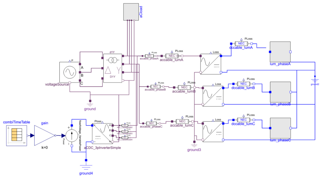
The designed upper-level template supports all three whole-building electrical architectures mentioned above and captures their electrical phases, control zones, and load types. It is similar to the simple upper-level template previously shown, with a three-phase input voltage source, a three-phase transformer, vectorized AC/DC converters connected to a vectorized lower-level load template on all three phases, three-phase AC loads, a PV system, and a three-phase inverter (Figure 12).

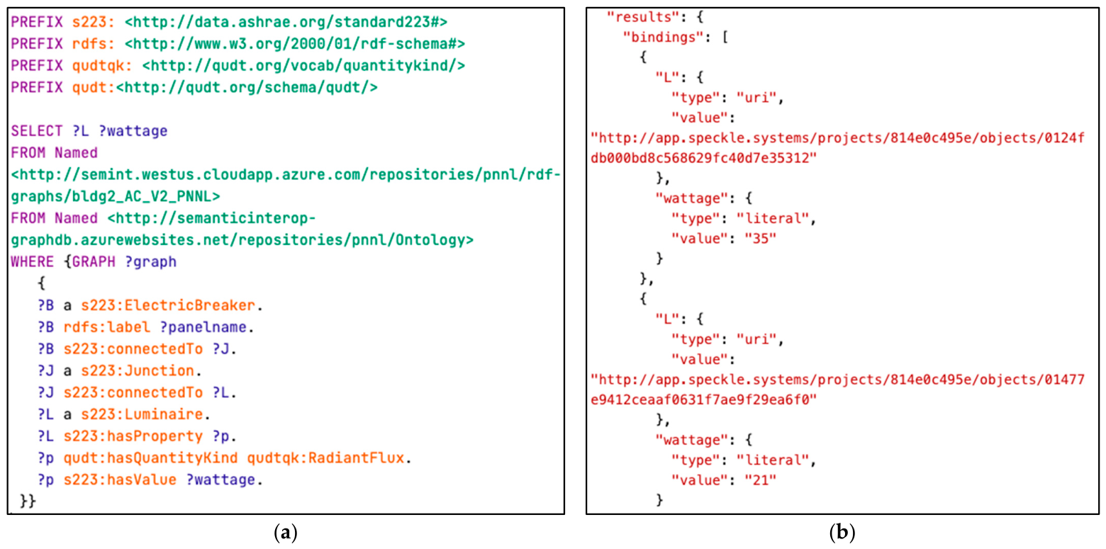
Data from a whole-building ASHRAE 223 semantic model is used to instantiate and assign parameter values to the template. A SPARQL query to the semantic model retrieves the electrical load information (e.g., load type, load specification, converter type, control zone) as a JSON object (Figure 13). Values assigned to each of the vectorized components determine the electrical architecture of the building.

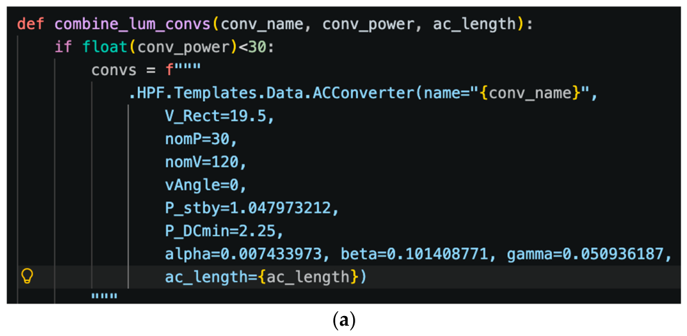
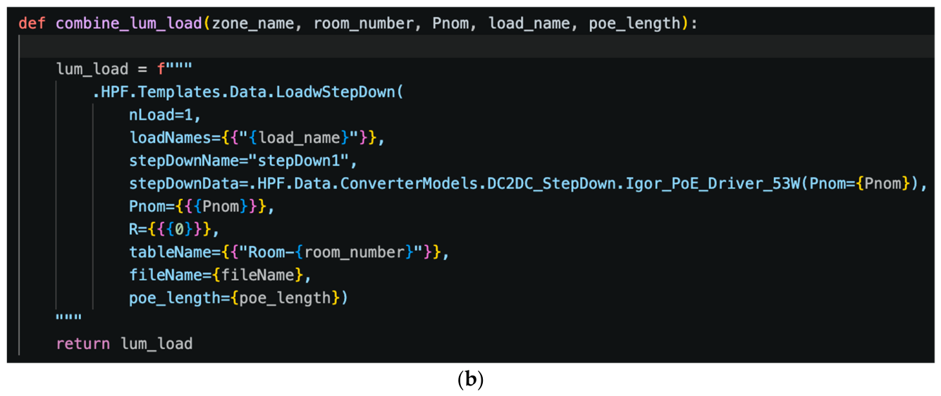
The semantic query output in JSON format is fed as an input to the Python middleware that generates a Modelica data record to instantiate the template. Functions are developed to generate blocks of text with parameter values for the vectorized components (Figure 14). Based on the number and types of devices and how they are connected, the Python 3.14 script uses these functions to generate the complete data record.

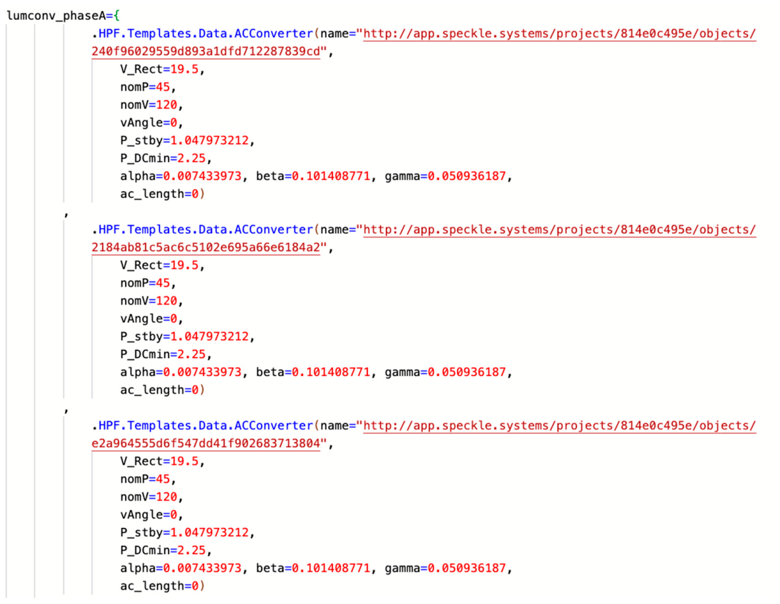
The generated data record has information about the number of AC/DC converters (e.g., LED drivers, PoE switches) in each phase, how many DC/DC converters and loads are connected to each AC/DC converter, the efficiency model and rated electrical data for each of the converters, and load schedules for each load (Figure 15).

To verify the template-based model generation method, the luminaire and MEL counts in the Modelica model were compared by rated load with those found in the ground truth Revit model (

Table 2. Whole-building workflow verification results.

Equipment Type	Rated Load	Revit Count	Modelica Count
Luminaire	13 W	9	9
	20 W	4	4
	21 W	88	88
	22 W	24	24
	25 W	52	52
	28 W	120	120
	31 W	352	352
	34 W	28	28
	35 W	28	28
	40 W	128	128
	42 W	20	20
Laptop	57 W	268	268
Monitor	46 W	268	268
Display	127 W	15	15
Printer	875 W	27	27

). The exact match observed for this whole-building model and its 1431 total devices demonstrates that the template-based approach can be applied to building electrical systems.

5. Case Study

Following the verification of the BEEAM Modelica library in previous work and the verification of RDF2EMO in this work, the ability of the proposed workflow to support design decisions in the SD and CD phases is demonstrated for the development of a reference medium office building. The building comprises 53,600 ft², three floors, 2 elevators, five thermal zones per floor, 204 lighting zones, 853 lighting fixtures, and 587 MELs. On-site energy storage and generation resources are considered for improving reliability when experiencing electric utility outages. Design support is demonstrated for system architecture and energy storage/generation resource sizing decisions.

Three system architectures are explored: AC-coupled energy storage and generation with AC lighting and MELs, AC-coupled energy storage and generation with DC lighting and MELs, and DC-coupled energy storage and generation with DC lighting and MELs. Each architecture is evaluated for energy losses, peak export, and reliability—using the metric of backup time following an outage.

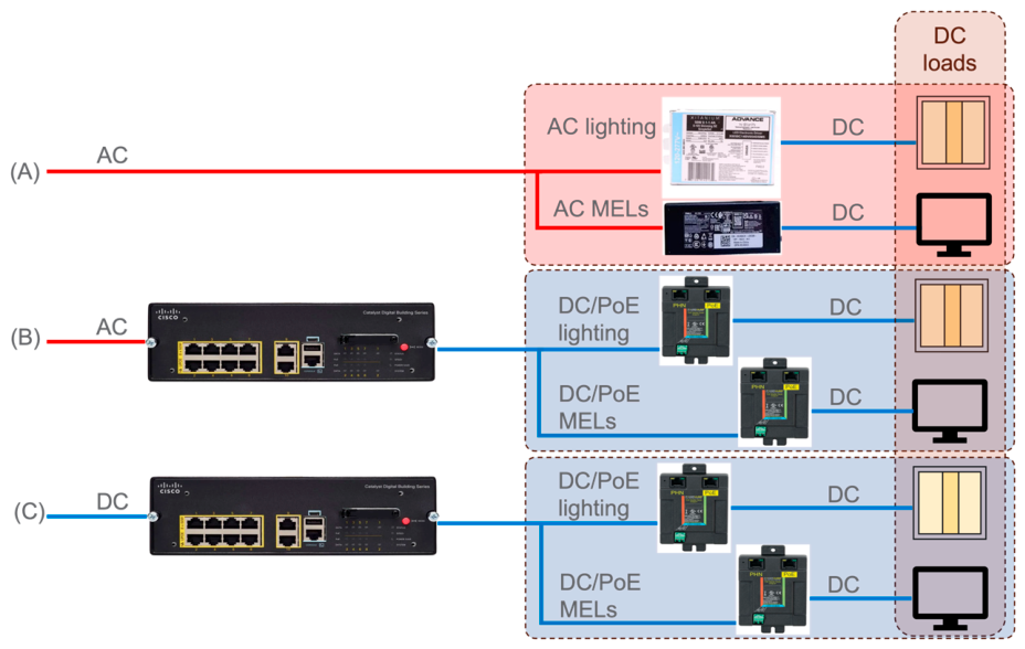
Lighting and MEL power flow details for all three system architectures are illustrated in Figure 16. In the AC-coupled architecture with AC lighting and MELs, AC power is distributed to AC/DC converters that produce the low-voltage DC power required by LED lighting loads and typical office MELs. In the AC-coupled architecture with DC lighting and MELs, AC power is distributed to PoE switches that convert AC power to low-voltage DC power. In the DC-coupled architecture with DC lighting and MELs, high-voltage DC power is distributed to PoE switches that convert high-voltage DC to low-voltage DC. The energy efficiency of the three architectures is affected by both converter efficiencies and wire types, lengths, and related losses.

5.1. SD Phase

5.1.1. Load, Breaker, and Wire Sizing

In the SD phase, HVAC and elevator loads are modeled based on actual equipment properties, while lighting loads and MELs are modeled for each space/zone based on industry reference power densities. The distribution of pure AC loads, DC loads powered via a DC/DC converter, and DC loads powered via an AC/DC converter is summarized as an AC:DC/DC:AC/DC ratio. Notably, in the SD phase model, lighting and MEL magnitudes do not vary by electrical distribution system architecture, and both DC-coupled architectures have the same AC:DC/DC:AC/DC ratio. SD phase loads are summarized in

Table 3. SD phase load summary.

Design Phase	System Architecture	HVAC Heating Load (kW)	HVAC Cooling Load (kW)	Elevator Load (kW)	Lighting Load (kW)	MELs (kW)	AC: DC/DC: AC/DC Ratio
SD	AC coupled	187.750	217.263	8.517	32.475	39.451	85:0:15
	DC coupled	187.750	217.263	8.517	32.475	39.451	85:15:0

. ElectroBIM calculates breaker sizes based on these load values and fire safety requirements (i.e., load values do not exceed 80% of the breaker rating) and performs voltage drop calculations for feeder and branch circuits, again ensuring fire safety requirements (i.e., less than a 3% voltage drop for feeders and 2% for branches) are met. If the calculated voltage drop exceeds the fire safety threshold, ElectroBIM automatically increases the wire size and updates the one-line diagram.

5.1.2. Peak and Average Demand

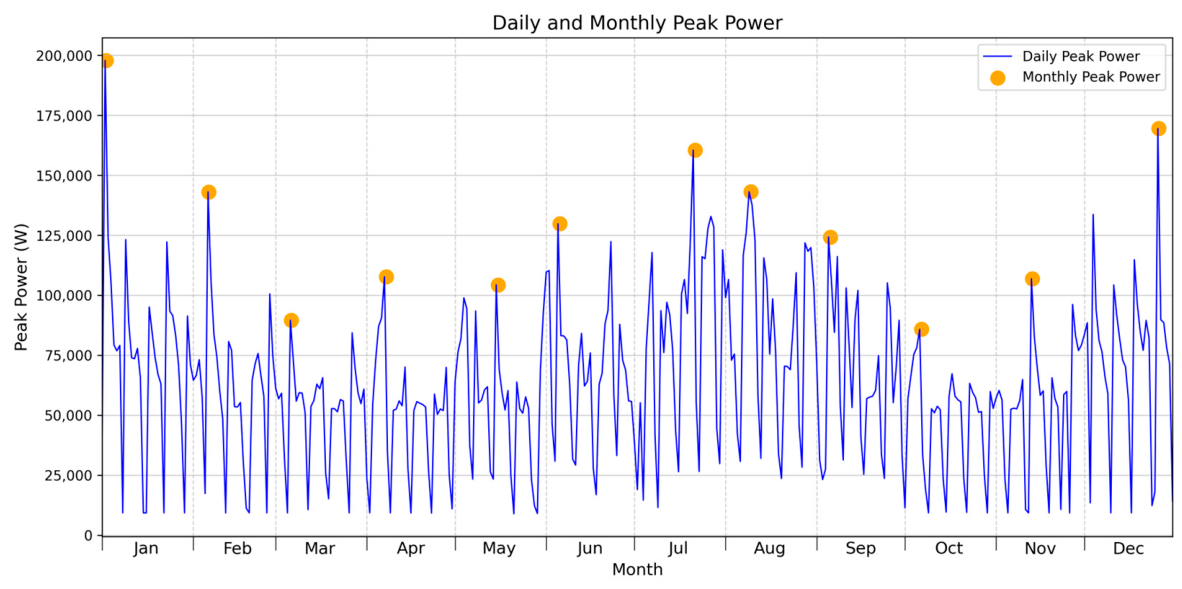
An SD-phase semantic model is generated from the Revit BIM with all parameter values. Using the template-based method, an SD Modelica model is generated directly from this semantic model. Electrical system power demand and energy use are inherently a function of how the systems are controlled and operated, and can be modeled with varying degrees of sophistication based on use-case needs. Given the simple approach to SD-phase load modeling (i.e., based on power densities), load control in this example is modeled by assigning simple schedules to all loads. The SD model is simulated for one year in Modelon Impact without any on-site generation or energy storage to determine daily and monthly peak loads (Figure 17). Simulation results are summarized in

Table 4. SD phase peak demand, average demand and average operational AC:DC/DC:AC/DC demand ratios, by load type, over a one-year simulation.

Design Phase	System Architecture	Peak HVAC Demand (kW)	Peak Elevator Demand (kW)	Peak Lighting Demand (kW)	Peak MEL Demand (kW)	Average HVAC Demand (kW)	Average Lighting +MEL Demand (kW)	Average AC:DC/DC: AC/DC Demand Ratio
SD	AC coupled	175.183	11.376	21.568	10.716	12.534	16.740	41:0:59
	DC coupled	175.183	11.376	21.568	10.716	12.534	16.740	41:59:0

.

5.1.3. Design Decisions

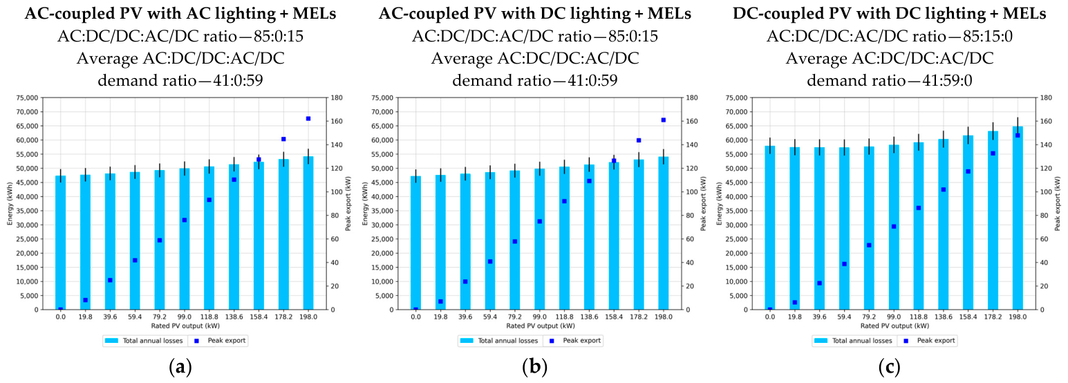
In this case study example, initial simulation results—for a design without any on-site generation and energy storage—are used to configure a second set of simulations that explore practical storage and generation sizing options. The size and range of this and any parametric study are inherently dependent on designer focus and constraints. In this example, four battery energy storage options (100 kWh, 250 kWh, 500 kWh, and 1000 kWh) and ten PV size options (spanning 10–100% of the estimated ~198 kW peak yearly building load) were evaluated. This second set of simulations is used to inform SD phase design decisions. Annual whole-building electrical losses (represented by blue bars) for the three system architectures under consideration are shown in Figure 18.

The AC-coupled PV with DC lighting + MELs architecture is estimated to be the most efficient for this building. Notably, this conclusion is highly dependent on multiple building design details, including its space types and sizes and corresponding system (e.g., lighting) requirements, AC:DC/DC:AC/DC ratios, and energy converter efficiencies. The DC-coupled architecture presents unique design considerations. Energy losses initially decrease as PV size increases, because PV initially serves DC loads via a more efficient energy converter. However, once PV generation exceeds DC demand, energy losses start increasing with further PV size increases, as the excess power routes through an AC/DC conversion to serve AC loads or export, introducing additional conversion loss.

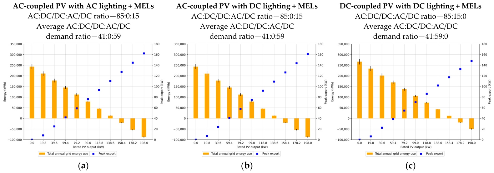
Simulation results indicate that increasing PV size reduces grid energy costs (orange bars) and increases peak energy export (blue squares), as illustrated in Figure 19.

Notably, simulation results do not reveal obvious deterministic design choices for this building. Rather, they enable the designer to make decisions based on quantitative analysis that should be notable improvements over qualitative comparisons, provided that modeling choices and assumptions (i.e., representative power density, control model) are suitable. The design of a building with both on-site storage and generation requires careful consideration of their intended uses and meaningful performance metrics. Furthermore, there is no single or best way to size both systems. For example, a designer might define and weigh multiple performance metrics and evaluate all parametric permutations through a mathematical optimization of the multi-metric analysis, or focus on one system at a time, along with the performance metric(s) that are most dependent on that system.

In this example, a version of that latter approach is pursued, focusing initially on sizing the PV system to meet a defined objective, and then sizing the battery energy storage system to meet a specific objective. The most suitable PV system size is determined by evaluating simulation results against two potential design objectives. In the first case, where a designer aims to restrict peak export to the grid interconnect agreement limit of 150 kW, a PV size of 178.2 kW might be selected for AC-coupled PV with DC lighting + MELs architecture. Alternatively, if the objective is to minimize annual grid energy consumption and associated costs, a PV size of 158.4 kW might be preferable for the same system architecture, as net grid energy use turns negative at this capacity—signifying that the building becomes a net exporter of energy.

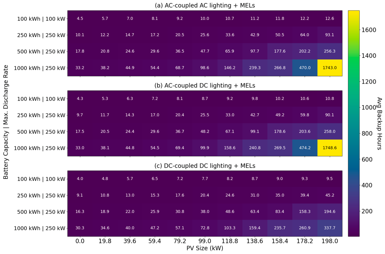
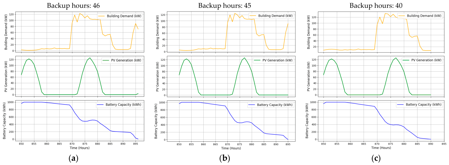
Continuing with the design approach for this case study, now that the PV system is sized, the most suitable battery energy storage system size is determined by evaluating simulation results against a single, more sophisticated design objective. In this example, the designer is focused on using the battery system solely to maximize building resilience to electrical outages; notably, this means that the battery is not discharged during normal grid operation. Multiple performance metrics might be considered, along with their dependencies on modeling choices and assumptions (i.e., control model). For this case study, a metric of average backup time over the course of a year is defined and evaluated for normal operation of the building (i.e., not altering the control of any of the building’s electrical systems to extend battery discharge duration). As a further simplification, the simple schedule-based load control model used for previous analyses is maintained. Average backup time is calculated by first simulating an outage at every hour of the year (again, with an assumption of normal building operation during the outage) and estimating how long the energy storage (and generation, if applicable) can continue to power the building, and then averaging this backup time for the entire year. Simulation results are shown in Figure 20. A representative outage scenario initiated at the 850th hour of the year, for a battery with a capacity of 1000 kWh and a maximum discharge rate of 250 kW, is shown for each system architecture in Figure 21.

In this example, simulation results reveal that for the previously selected system architecture (AC-coupled PV with DC lighting + MELs) and candidate PV sizes (158.4 kW and 178.2 kW), a battery with a 500 kWh capacity is needed to achieve a design target of one week of backup time (i.e., 168 h).

5.2. CD Phase

In the CD phase, designs typically become more detailed as building architectural details are finalized (e.g., individual rooms/spaces, lighting and HVAC service zones), and equipment load estimates based on industry-reference power densities are replaced by actual equipment ratings.

5.2.1. Load, Breaker, and Wire Sizing

ElectroBIM recalculates breaker sizes based on the updated loads, performs voltage-drop calculations using wire lengths, and enforces 3%/2% feeder/branch limits. Where the voltage drop exceeds the threshold, ElectroBIM automatically increases the wire size, producing an optimized one-line diagram. SD and CD phase loads for this case study example are summarized in

Table 5. SD and CD phase load summary.

Design Phase	System Architecture	HVAC Heating Load (kW)	HVAC Cooling Load (kW)	Elevator Load (kW)	Lighting Load (kW)	MEL Load (kW)	AC: DC/DC: AC/DC Ratio
SD	AC coupled	187.750	217.263	8.517	32.475	39.451	85:0:15
	DC coupled	187.750	217.263	8.517	32.475	39.451	85:15:0
CD	AC coupled	187.750	217.263	8.517	25.841	58.723	82:0:18
	DC coupled	187.750	217.263	8.517	25.841	58.723	82:12:6

. The AC load (HVAC and elevator) is unchanged, while the modest reduction in lighting load is offset by a more significant increase in MELs, resulting in a small change in the AC:DC/DC:AC/DC load ratios.

5.2.2. Peak and Average Demand

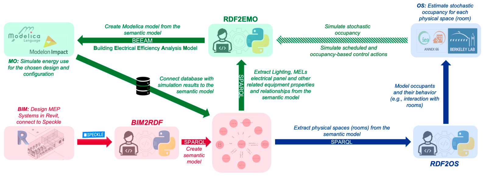
A CD phase semantic model is generated from the CD phase Revit BIM using BIM2RDF, as described previously. A CD phase Modelica model is generated from this semantic model using RDF2EMO, as described previously. As the AC loads (HVAC and elevators) remain unchanged from SD to CD, their control is again modeled by assigning simple schedules. Given the more detailed approach to CD-phase DC load modeling (i.e., actual equipment ratings), load control is modeled using an occupancy-based strategy, rather than the simple schedule-based approach used for the SD phase analysis. A previously developed tool (RDF2OS) is used to extract physical information from the semantic model and semi-automatically generate stochastic occupancy models for each space in the building, as well as the occupant types (e.g., manager, custodian). The models are simulated using a previously developed occupancy simulator (Figure 22) [29].

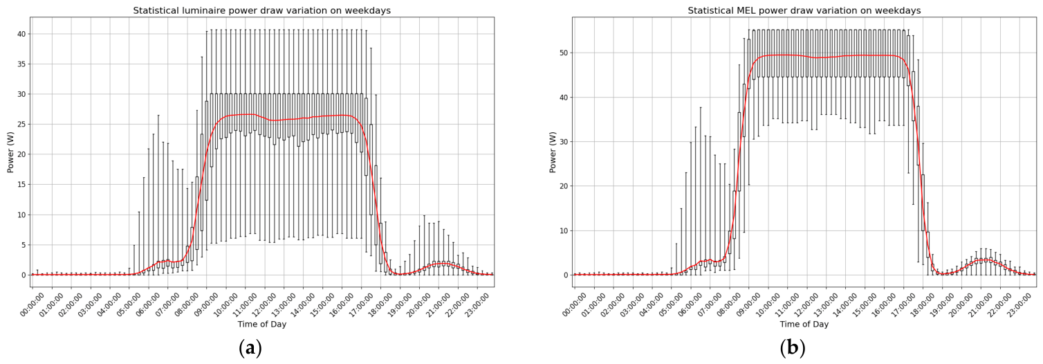
An occupancy-based control strategy can be designed and modeled with varying degrees of sophistication based on use-case needs. In this example, a simple approach is used, whereby all lighting and MELs in a control zone are turned ON if the zone is occupied and turned OFF when the zone is unoccupied. Human occupancy sensing is assumed to be ideal (i.e., if the control zone is occupied, the sensor perfectly detects occupancy with no false positives or negatives). The statistical weekday power demand for lighting loads and MELs that results from the simulation of this occupancy-based control strategy for a period of one year is shown in Figure 23.

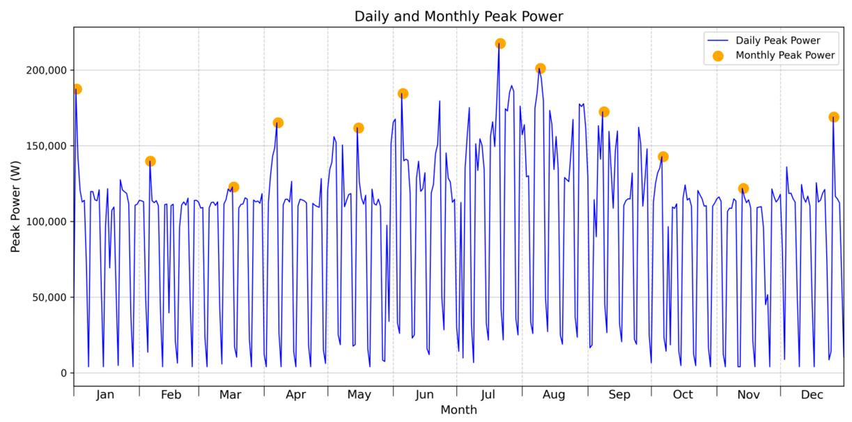
The CD model is simulated for one year in Modelon Impact without any on-site generation or storage to refine the daily and monthly peak load estimates (Figure 24). Notably, the peak yearly demand estimate increases from 198 kW to 218 kW, while the average yearly demand increases from 29.26 kW to 38.99 kW.

Simulation results are summarized in

Table 6. SD and CD phase peak demand, average demand, and average AC:DC/DC:AC/DC demand ratios over a one-year simulation.

Design Phase	System Architecture	Peak HVAC Demand (kW)	Peak Elevator Demand (kW)	Peak Lighting Demand (kW)	Peak MEL Demand (kW)	Average HVAC Demand (kW)	Average Lighting + MEL Demand (kW)	Average AC:DC/DC: AC/DC Demand Ratio
SD	AC coupled	175.183	11.376	21.568	10.716	12.534	16.740	41:0:59
	DC coupled	175.183	11.376	21.568	10.716	12.534	16.740	41:59:0
CD	AC coupled	175.183	11.376	25.066	57.325	12.534	25.878	72:0:28
	DC coupled	175.183	11.376	25.066	57.325	12.534	25.878	72:24:4

. The CD phase demand ratios are significantly different from the SD phase ratios for both system architectures, revealing the impact of higher lighting and MEL demand that results from a net higher rated load and the change from a simple schedule-based control to an occupancy-based control strategy.

5.2.3. Design Decisions

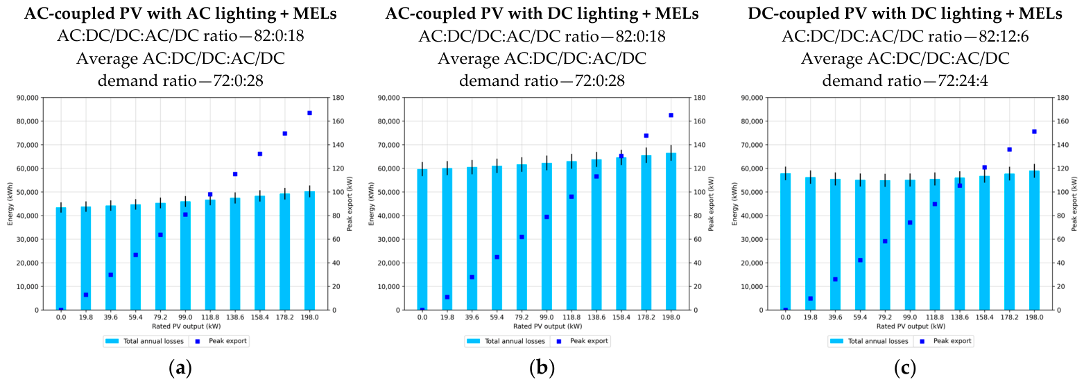
Continuing with this case study example, the exploration of practical generation and storage sizing options is updated for the CD phase designs using the same approach and parametric variations as were used for the SD phase design. Updated annual whole-building electrical losses for the three system architectures under consideration are shown in Figure 25.

The updated analysis reveals that the AC-coupled PV with AC lighting + MELs architecture is now estimated to be the most efficient for this building, a change from the SD phase design choice of an AC-coupled PV with DC lighting + MELs architecture.

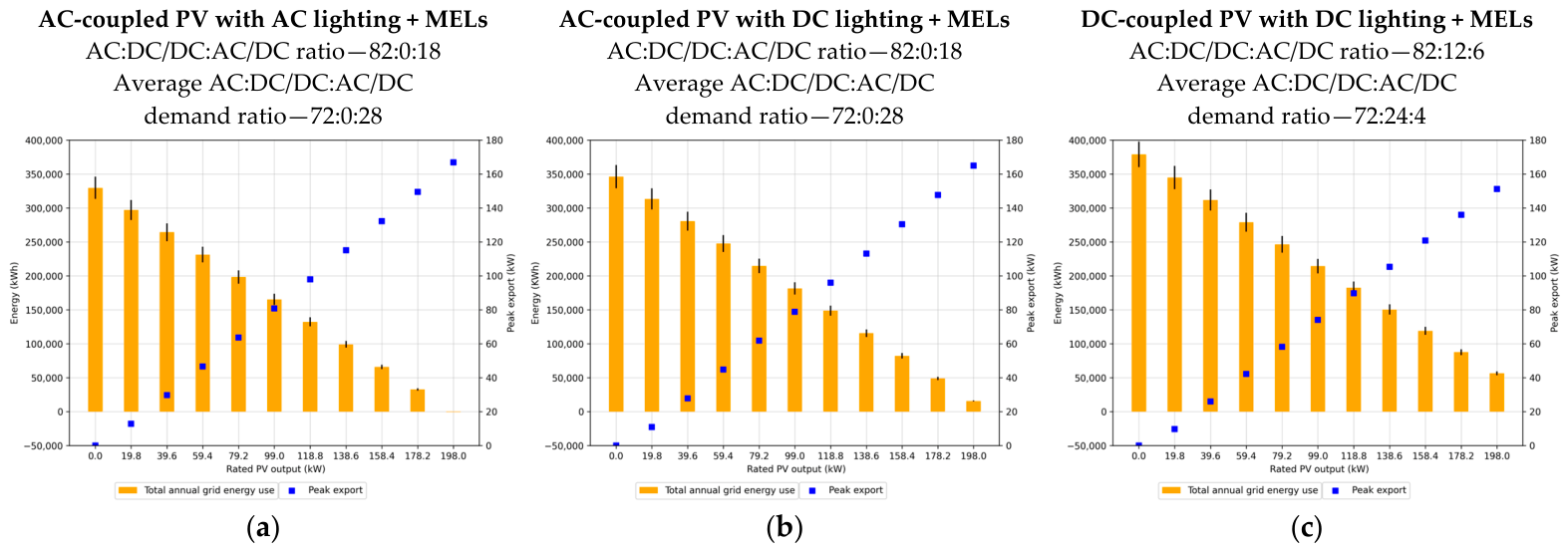
In this example, the SD phase approach of focusing initially on sizing the PV system is pursued in the CD phase as well. The most suitable PV system size is refined by evaluating simulation results against the same two design objectives (Figure 26). In the first case, where a designer aims to restrict the peak export to the grid interconnect agreement limit of 150 kW, a PV size of 158.4 kW might be selected for the AC-coupled PV with AC lighting + MELs architecture. Alternatively, if the objective is to minimize annual grid energy consumption and associated costs, a PV size of 198.0 kW might be preferable for the same system architecture, as the net grid energy use turns negative at this capacity—signifying that the building becomes a net exporter of energy.

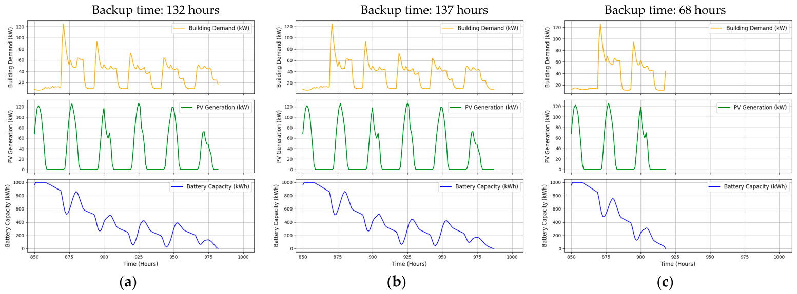
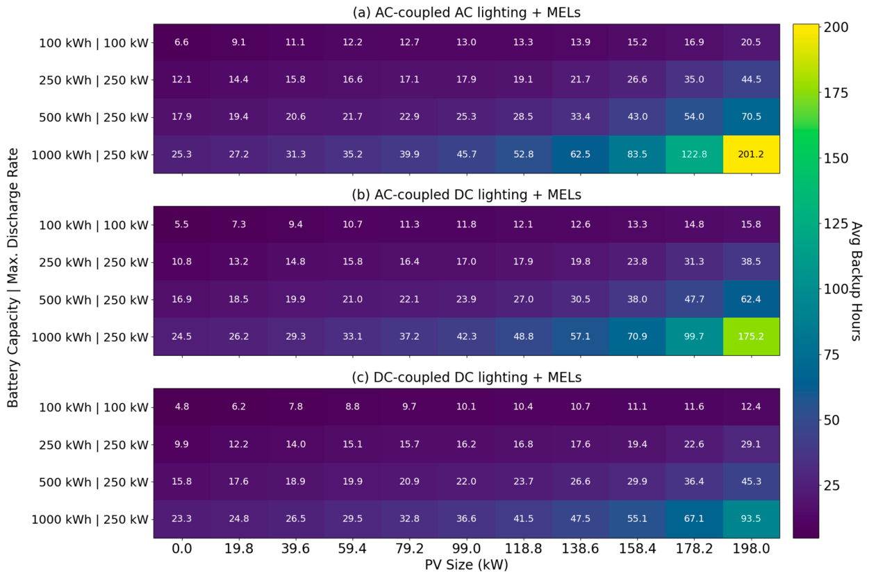
Following the PV system size revision, the most suitable battery energy storage system size is determined by evaluating simulation results against the same single design objective: to maximize building resilience to electrical outages. The SD-phase metric of average backup time over the course of a year is evaluated for normal operation of the building, using the updated modeling of normal operation and associated simulation results described previously (i.e., simple schedule-based load control for AC loads and occupancy-based load control for DC loads). Simulation results are shown in Figure 27. A representative outage scenario initiated at the 850th hour of the year for a battery with a capacity of 1000 kWh and a maximum discharge rate of 250 kW is shown for each system architecture in Figure 28.

Simulation results for this case study reveal that for the previously selected system architecture (AC-coupled with AC lighting + MELs) and peak-export limiting PV size (158.4 kW), a battery bigger than 1000 kWh capacity is needed, as none of the simulated battery sizes was able to provide the targeted one week of backup time (i.e., 168 h). However, for the grid energy cost minimizing PV size (198 kW), a 1000 kWh capacity is found to be sufficient.

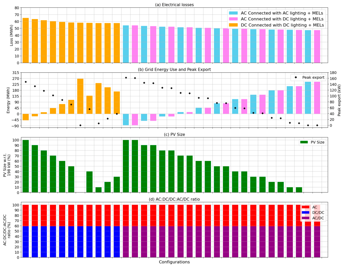
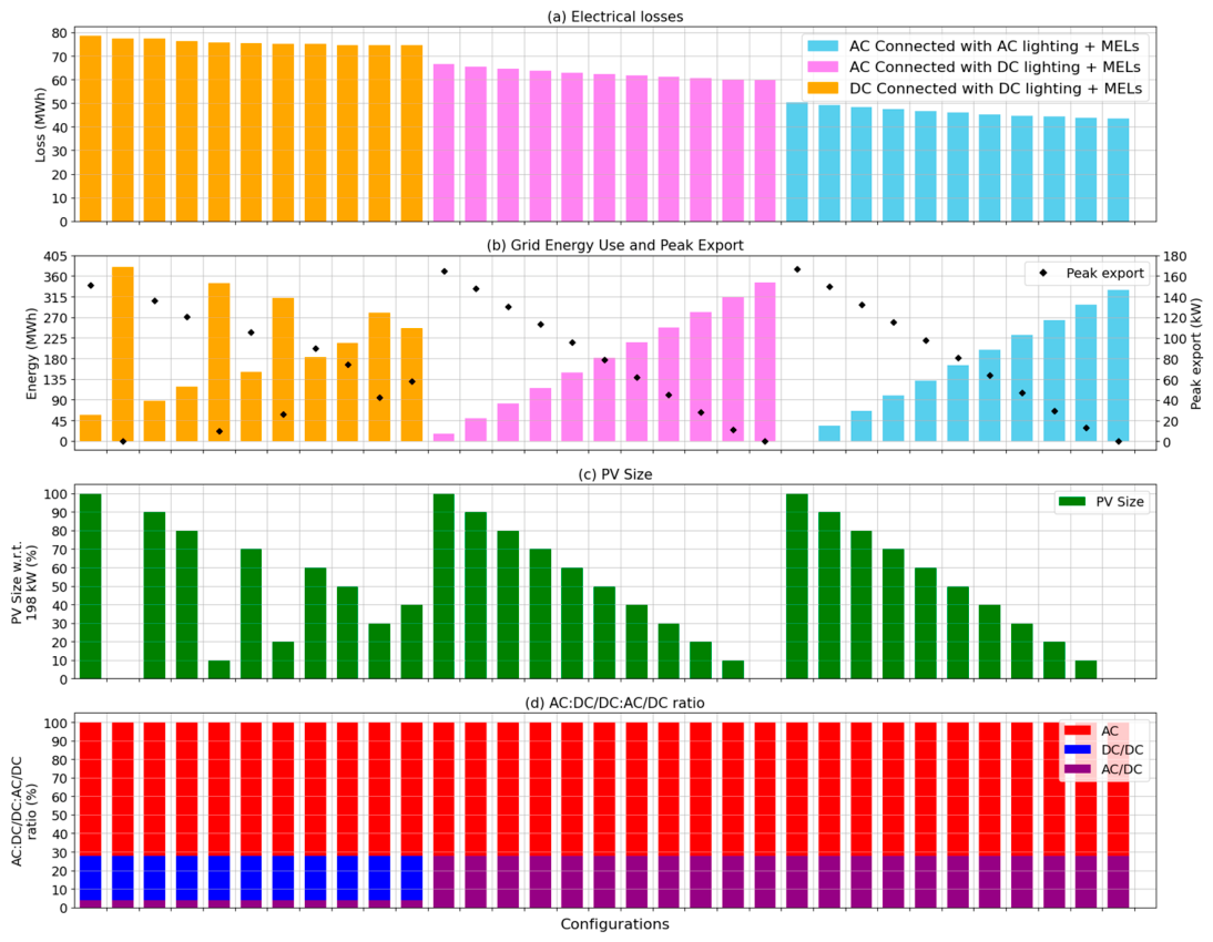
Simulation results for the SD and CD phases are summarized in Figure 29 and Figure 30 by visualizing the electrical losses that result from all simulated system architecture and PV size configurations. This case study example demonstrates that optimal design decisions are dynamic and may change as the project progresses through various phases, highlighting the importance of performing simulations at each stage of the design process. It is important to note that performance metrics and corresponding design choices cannot be universally applied; rather, they are influenced by design and modeling choices, including system architecture details, equipment ratings, and control strategies. Therefore, simulation and careful analysis are essential to inform decisions tailored to the unique needs of each project. Notably, the comparison of configurations that lead to design decisions is dependent on the modeling detail, assumptions, and accuracy. While modeling and simulation facilitate quantitative analyses and comparisons that can be better than qualitative ones, they are subject to choices made by the modeler. For example, the case study presented here modeled load control as simple schedules that integrated one or more underlying control strategies or a single occupancy-based strategy for all lighting and MELs; both are simplifications of real-world systems that may or may not have significant implications for simulation accuracy and configuration comparisons. Similarly, while the power converter efficiencies in the utilized Modelica models were derived from the characterization of representative real-world equipment (e.g., luminaires, computers), they may or may not be representative of the equipment that is actually installed in the building—especially if there is wide variation in market-available equipment or a significant improvement in technology over time that is not captured by updates to the models or the model library.

6. Conclusions

This paper presents a comprehensive workflow for designing modern building electrical systems. The workflow seamlessly connects Building Information Models, semantic models, and Modelica simulation models. It supports AC, DC, and hybrid AC + DC electrical systems as well as energy storage and generation systems, and is suitable for evaluating designs as they progress from typical SD to CD phases. A new Python middleware tool, RDF2EMO, is described in detail. It leverages a template-based approach to semi-automate Modelica model generation from a semantic model. This automation significantly reduces modeling effort, enables the consideration of more design choices, and improves design decision confidence. Verification of RDF2EMO using a reference medium office building demonstrates that the generated Modelica model is internally consistent with the Building Information Model.

The workflow supports data-driven decision-making throughout the design process by enabling designers to evaluate electrical system behaviors, analyze architectural tradeoffs, and evaluate the impact of equipment characteristics (e.g., power conversion efficiency) and sizing (e.g., energy storage or generation capacity). Automation allows more options to be considered in early design phases and more details to be captured in later design phases, thereby ensuring that the decisions made in early design phases remain justified as the design becomes more mature and detailed.

The included case study example demonstrates these workflow capabilities and provides evidence for accepting the hypothesis that motivated this work—that modern building electrical system complexity and design choices warrant the use of modeling and simulation tools. Notably, the case study results do not provide evidence that any particular modeling choice or design decision is right or wrong or can be directly applied to other designs—and the reader is cautioned against inferring or otherwise drawing such conclusions. Rather, the presented case study aims to demonstrate the interdependent relationship between modeling choices and assumptions, design choices, and performance objectives—and the ability of the workflow to quantify the impact of these choices, assumptions, and objectives. The importance of modeling choices and assumptions can be revealed by examining the impact of changing from simple energy-density based load models and schedule-based load control models in the SD phase to equipment-based load models and an occupancy-based load control model in the CD phase. The interdependent relationship between design choices can be revealed by examining the impact of system architecture and energy generation capacity on system energy losses. The importance of performance objectives can be revealed by examining the impact on PV system capacity of a focus on peak export vs. grid energy use. Finally, multiple interdependencies can be revealed in the approach taken towards sizing the battery energy storage system, including the choice of performance objectives (i.e., focusing only on resilience to electrical outages), performance metrics (i.e., average backup time), and the approach taken to making design decisions (i.e., sequencing decisions with a focus on specific objectives). It is likely that different design choices would be made if different performance objectives and metrics were used, or if a different design approach was employed.

This paper does not intend to imagine or execute a definitive parametric analysis over an exhaustive modeling and design space that spans all possible permutations; on the contrary, it proposes that such an analysis is impractical for a practitioner and perhaps even impossible for a researcher. Rather, we propose that there is a happy medium between such a comprehensive quantitative approach and conventional approaches that often (a) rely on inherently limited recommended practices and qualitative analysis, (b) learn by project-by-project trial and error, and (c) over-emphasize risk and responsibility management by siloing legal responsibilities. This happy medium integrates designer choice and experience with tools and workflows that allow the designer to quantify the impacts of chosen areas of focus, and create feedback loops that drive performance improvement faster than typical project-by-project trial and error lessons. For example, if—as in the presented case study—occupant behavior is known or believed to have a significant impact on system performance, then occupancy behavior can be modeled to varying degrees of fidelity. If control strategy performance is paramount, then the designer might pursue higher-fidelity modeling of control strategies than those presented in the case study—perhaps accounting for sensor degradation or the probability of false positives or negatives. Similarly, if equipment technology is improving significantly or the market offers a wide range of performance, they might pursue the use of equipment-specific models rather than generic, representative models. The key imagined benefit of the presented tools and workflow is indeed in the ability to define and create customized, meaningful feedback loops that span design, construction, and operation.

In summary, the workflow provides designers and operators with a scalable and adaptable modeling framework that reduces manual effort and potentially improves design decision confidence. Furthermore, the incorporation of semantic modeling and the leveraging of modern semantic modeling approaches (i.e., the use of semantic web technologies by ASHRAE 223), facilitates the future extension of the workflow to yield true “digital twins” that are capable of directly and easily comparing design estimates with operational truths. Digital twins have long promised the ability to both improve building performance over the course of its operation and improve design practices while reducing development costs over the course of multiple projects. However, multiple real-world challenges have limited digital twins from realizing this potential, notably including excessive time and effort required to create them. The workflow described here can potentially reduce this time and effort by integrating digital twin creation into existing industry practices.

References

1. Gerber, D.L.; Vossos, V.; Feng, W.; Marnay, C.; Nordman, B.; Brown, R. A Simulation-Based Efficiency Comparison of AC and DC Power Distribution Networks in Commercial Buildings. Appl. Energy 2018, 210, 1167–1187. [Google Scholar] [CrossRef]
2. Vossos, V.; Gerber, D.L.; Gaillet-Tournier, M.; Nordman, B.; Brown, R.; Heredia, W.B.; Ghatpande, O.; Saha, A.; Arnold, G.; Frank, S.M. Adoption Pathways for DC Power Distribution in Buildings. Energies 2022, 15, 786. [Google Scholar] [CrossRef]
3. Vossos, V.; Garbesi, K.; Shen, H. Energy Savings from Direct-DC in U.S. Residential Buildings. Energy Build. 2014, 68, 223–231. [Google Scholar] [CrossRef]
4. Autodesk Revit. Available online: https://www.Autodesk.Com/Products/Revit/Overview (accessed on 12 May 2026).
5. ETAP. Available online: https://www.Etap.Com/Home (accessed on 12 May 2026).
6. EasyPower. Available online: https://www.Easypower.Com/Products/Easypower (accessed on 12 May 2026).
7. Sacks, R.; Eastman, C.; Lee, G.; Teicholz, P. BIM Handbook: A Guide to Building Information Modeling for Owners, Designers, Engineers, Contractors, and Facility Managers; Wiley: Hoboken, NJ, USA, 2018; ISBN 978-1-119-28753-7. [Google Scholar] [CrossRef]
8. Frank, S.; Ball, B.; Ghatpande, O.; Cale, J.; Othee, A. BEEAM (Building Electrical Efficiency Analysis Model), [SWR-20-107]; Colorado State University Research Foundation (CSURF), National Renewable Energy Laboratory (NREL): Golden, CO, USA, 2020. [Google Scholar]
9. DesignMaster Software. ElectroBIM. Available online: https://www.Designmaster.Biz/Revit/ (accessed on 12 May 2026).
10. SKM. Available online: https://www.Skm.Com/Index.Html (accessed on 12 May 2026).
11. Siemens. PSS®E. Available online: https://www.Siemens.Com/Us/En/Products/Energy/Grid-Software/Planning/Pss-Software/Pss-e.Html (accessed on 12 May 2026).
12. PowerWorld Corporation. PowerWorld. Available online: https://www.Powerworld.Com/ (accessed on 12 May 2026).
13. Zimmerman, R.D.; Murillo-Sánchez, C.E. MATPOWER, version 8.1; Cornell University: Ithaca, NY, USA, 2025. [Google Scholar]
14. De Castro, M.; Winkler, D.; Laera, G.; Vanfretti, L.; Dorado-Rojas, S.A.; Rabuzin, T.; Mukherjee, B.; Navarro, M. Version [OpenIPSL 2.0.0]—[iTesla Power Systems Library (iPSL): A Modelica Library for Phasor Time-Domain Simulations]. SoftwareX 2023, 21, 101277. [Google Scholar] [CrossRef]
15. Nytsch-Geusen, C.; Inderfurth, A.; Kaul, W.; Mucha, K.; Rädler, J.; Thorade, M.; Ribas Tugores, C. Template Based Code Generation of Modelica Building Energy Simulation Models. In Proceedings of the 12th International Modelica Conference, Prague, Czech Republic, 15–17 May 2017; pp. 199–207. [Google Scholar] [CrossRef]
16. Gautier, A.; Wetter, M.; Hu, J.; Tummescheit, H. HVAC and Control Templates for the Modelica Buildings Library. Model. Conf. 2023, 217–228. [Google Scholar] [CrossRef]
17. Nytsch-Geusen, C.; Rädler, J.; Thorade, M.; Ribas Tugores, C. BIM2Modelica—An Open Source Toolchain for Generating and Simulating Thermal Multi-Zone Building Models by Using Structured Data from BIM Models. In Proceedings of the 13th International Modelica Conference 33, Regensburg, Germany, 4–6 March 2019; pp. 33–38. [Google Scholar] [CrossRef]
18. Andriamamonjy, A.; Saelens, D.; Klein, R. An Automated IFC-Based Workflow for Building Energy Performance Simulation with Modelica. Autom. Constr. 2018, 91, 166–181. [Google Scholar] [CrossRef]
19. Aldosari, M.; Govertsen, K.; Central, P.D.; Poplawski, M.; Gupta, T. Pacific Northwest National Laboratory (PNNL), Richland, WA (United States). Pnnl/BIM2RDF. Available online: https://www.Osti.Gov/biblio/code-150523 (accessed on 19 March 2026).
20. Speckle. Available online: https://speckle.systems/ (accessed on 15 May 2026).
21. Waghale, A.; Pratoomratana, S.; Poplawski, M. Demonstration of a Modeling Toolkit for the Design of Building Electrical Distribution Systems. In Proceedings of the 9th ACM International Conference on Systems for Energy-Efficient Buildings, Cities, and Transportation, Boston, MA, USA, 9 November 2022; pp. 246–249. [Google Scholar] [CrossRef]
22. Waghale, A.; Pratoomratana, S.; Woodstock, T.-K.; Devaprasad, K.; Poplawski, M. Verification of a Modeling Toolkit for the Design of Building Electrical Distribution Systems. Buildings 2023, 13, 2520. [Google Scholar] [CrossRef]
23. Frank, S.M.; Ghatpande, O.; Shackelford, J.; Steen, M.; Ball, B.L.; Gerber, D.L.; Santos, A.; Brown, R.E. Experimental Validation of a Co-Simulation Architecture for Modeling Whole-Building and Detailed Electrical Distribution Performance. Energy Build. 2025, 344, 115917. [Google Scholar] [CrossRef]
24. Modelon. Modelon Impact. Available online: https://www.Modelon.Com/Modelon-Impact/ (accessed on 12 May 2026).
25. Dassault Systemes. Dymola Systems Engineering. Available online: https://www.3ds.Com/Products/Catia/Dymola (accessed on 12 May 2026).
26. Othee, A.; Cale, J.; Santos, A.; Frank, S.; Zimmerle, D.; Ghatpande, O.; Duggan, G.; Gerber, D. A Modeling Toolkit for Comparing AC and DC Electrical Distribution Efficiency in Buildings. Energies 2023, 16, 3001. [Google Scholar] [CrossRef]
27. Fritzson, P.; Pop, A.; Abdelhak, K.; Ashgar, A.; Bachmann, B.; Braun, W.; Bouskela, D.; Braun, R.; Buffoni, L.; Casella, F.; et al. The OpenModelica Integrated Environment for Modeling, Simulation, and Model-Based Development. Model. Identif. Control 2020, 41, 241–295. [Google Scholar] [CrossRef]
28. U.S. DOE BTO Building Energy Codes Program Prototype Building Models. 2021. Available online: https://www.energycodes.gov/prototype-building-models (accessed on 24 May 2026).
29. Dehwah, A.H.; Devaprasad, K.; Woodstock, T.K.A.; Gupta, T.; Passmore, M.N.; Poplawski, M.E. A BIM-BEM Based Workflow for Designing Integrated HVAC and Lighting Systems. ASHRAE Trans. 2026, 132, 1395–1406. [Google Scholar] [CrossRef]
Figure 1. A proposed workflow that automates the generation of Modelica models from BIM data via a semantic model.
Energies 19 02586 g001
Figure 2. An automated approach for the generation of a Modelica model using two-level model templates and Python.
Energies 19 02586 g002
Figure 3. Two four-luminaire lighting systems modeled using the template-based approach and BEEAM, and simulated in Modelon Impact.
Energies 19 02586 g003
Figure 4. (a) A distributed DC/PoE four-luminaire lighting system modeled in Modelon Impact using BEEAM; (b) a simple lower-level load template.
Energies 19 02586 g004
Figure 5. (a) A conventional AC four-luminaire lighting system modeled in Modelon Impact using BEEAM; (b) a simple lower-level load template.
Energies 19 02586 g005
Figure 6. (a) A simple upper-level template with vectorized components that can be instantiated to achieve multiple system architectures; (b) a simple lower-level load template with vectorized components.
Energies 19 02586 g006
Figure 7. A Modelica data record used to instantiate the distributed DC/PoE four-luminaire lighting system model.
Energies 19 02586 g007
Figure 8. Comparison of the simulated input power draw of the four-luminaire lighting system model in (a) conventional AC and (b) distributed DC architecture when modeled via the manual approach (orange) vs. the template approach (blue).
Energies 19 02586 g008
Figure 9. Conventional AC architecture for the reference medium office building with an AC/DC converter at each end-use device.
Energies 19 02586 g009
Figure 10. Distributed PoE architecture for the reference medium office building with AC/DC converters (PoE switches) installed in a distributed configuration near loads.
Energies 19 02586 g010
Figure 11. Centralized PoE architecture for the reference medium office building with AC/DC converters (PoE switches) installed in a centralized configuration.
Energies 19 02586 g011
Figure 12. Upper-level template for the reference medium office building that supports three electrical architectures.
Energies 19 02586 g012
Figure 13. SPARQL query to the semantic model (a) and the output snapshot in JSON format (b).
Energies 19 02586 g013
Figure 14. Python 3.14 functions for (a) converter and (b) load that generate a data record from the semantic query output.
Energies 19 02586 g014aEnergies 19 02586 g014b
Figure 15. Modelica data record snapshot generated using Python 3.14, which is used to instantiate the medium office building model template.
Energies 19 02586 g015
Figure 16. Lighting and MEL power flow for three system architectures: (A) AC-coupled PV with AC lighting and MELs, (B) AC-coupled PV with DC lighting and MELs, and (C) DC-coupled PV with DC lighting and MELs.
Energies 19 02586 g016
Figure 17. SD phase daily (blue) and monthly (orange) peak demand.
Energies 19 02586 g017
Figure 18. SD phase annual electrical losses (blue bars) and peak PV export (blue squares), as a function of PV size and system architecture: (a) AC-coupled PV with AC lighting + MELs, (b) AC-coupled PV with DC lighting + MELs and (c) DC-coupled PV with DC lighting + MELs.
Energies 19 02586 g018
Figure 19. SD phase annual energy use (orange bars) and peak PV export (blue squares) as a function of PV size and systems architecture: (a) AC-coupled PV with AC lighting + MELs, (b) AC-coupled PV with DC lighting + MELs and (c) DC-coupled PV with DC lighting + MELs.
Energies 19 02586 g019
Figure 20. SD phase average backup time in hours for four battery sizes, 11 PV sizes, and three system architectures: (a) AC-coupled PV with AC lighting + MELs, (b) AC-coupled PV with DC lighting + MELs and (c) DC-coupled PV with DC lighting + MELs.
Energies 19 02586 g020
Figure 21. An SD phase representative outage scenario initiated at the 850th hour of the year, utilizing a battery capacity of 1000 kWh and a 250 kW discharge rate for each architecture: (a) AC-coupled PV with AC lighting + MELs, (b) AC-coupled PV with DC lighting + MELs and (c) DC-coupled PV with DC lighting + MELs.
Energies 19 02586 g021
Figure 22. Workflow for modeling and simulating stochastic occupancy for the CD phase model using the RDF2OS tool and an occupancy simulator.
Energies 19 02586 g022
Figure 23. CD phase statistical weekday power demand for (a) lighting and (b) MELs when subjected to a simple occupancy-based control strategy for a period of one year.
Energies 19 02586 g023
Figure 24. CD phase daily (blue) and monthly (orange) peak demand.
Energies 19 02586 g024
Figure 25. CD phase annual electrical losses (blue bars) and peak PV export (blue squares), as a function of PV size and system architecture: (a) AC-coupled PV with AC lighting + MELs, (b) AC-coupled PV with DC lighting + MELs and (c) DC-coupled PV with DC lighting + MELs.
Energies 19 02586 g025
Figure 26. CD phase annual energy use (orange bars) and peak PV export (blue squares) as a function of PV size and system architecture: (a) AC-coupled PV with AC lighting + MELs, (b) AC-coupled PV with DC lighting + MELs and (c) DC-coupled PV with DC lighting + MELs.
Energies 19 02586 g026
Figure 27. CD phase average backup time in hours for four battery sizes, 11 PV sizes, and three system architectures: (a) AC-coupled PV with AC lighting + MELs, (b) AC-coupled PV with DC lighting + MELs and (c) DC-coupled PV with DC lighting + MELs.
Energies 19 02586 g027
Figure 28. A CD phase representative outage scenario initiated at the 850th hour of the year, utilizing battery capacity of 1000 kWh and discharge rate of 250 kW for each architecture: (a) AC-coupled PV with AC lighting + MELs, (b) AC-coupled PV with DC lighting + MELs and (c) DC-coupled PV with DC lighting + MELs.
Energies 19 02586 g028
Figure 29. SD phase whole-building simulation results: (a) electrical losses ordered from highest to lowest, (b) grid energy use and peak export, (c) PV size, and (d) AC:DC/DC:AC/DC ratio for all system architectures and PV size configurations.
Energies 19 02586 g029
Figure 30. CD phase whole-building simulation results: (a) electrical losses ordered from highest to lowest, (b) grid energy use and peak export, (c) PV size, and (d) AC:DC/DC:AC/DC ratio for all system architectures and PV size configurations.
Energies 19 02586 g030