A Unified Methodology for Direct and Inverse Problems in Steady-State Thermal–Hydraulic Networks

Abstract

Steady-state thermal–hydraulic network models are widely used for the analysis, design, and operation of energy systems. While direct problems with prescribed boundary conditions can often be solved efficiently, inverse problems such as set-point tracking and parameter identification are commonly addressed through repeated solution of the corresponding direct problem. For large-scale networks with strong nonlinear couplings, such nested strategies can become computationally expensive and numerically burdensome. This paper presents a unified methodology for the solution of direct and inverse steady-state thermal–hydraulic problems within a single modeling workflow. In contrast to classical nested approaches, inverse problems are formulated in a simultaneous analysis and design framework, in which system states and selected system inputs are treated as unknowns simultaneously. The methodology combines externally causal component representations with acausal network balance relations in order to expose the structural dependencies of the assembled system and enable graph-based tearing reduction. Component-local evaluations, including possible component-internal nonlinear calculations, are encapsulated within the component models, while the nonlinear network closure problem is restricted to a reduced set of tearing variables.. Direct problems are solved by nonlinear root finding on the tearing-reduced residual system, whereas inverse problems are posed as tearing-reduced residual-constrained nonlinear programs with equality, inequality, and bound constraints. The methodology is demonstrated on a vapor-compression refrigeration cycle, where compressor speed and expansion valve opening are adjusted to satisfy prescribed cooling-load and superheat targets under varying condenser inlet temperatures. Implemented in Python, the proposed methodology supports transparent and reproducible modeling and provides a practical basis for simulation, set-point tracking, and constrained optimization of coupled thermal–hydraulic networks.

1. Introduction

Thermal–hydraulic energy systems play an important role in the ongoing transformation of heating, cooling, refrigeration, and industrial process infrastructures. Heat pumps, refrigeration cycles, geothermal systems, district heating and district cooling networks, and thermal process plants are expected to provide efficient energy conversion, integrate renewable and waste-heat sources, and operate flexibly under changing boundary conditions. The International Energy Agency identifies energy efficiency, electrification, and flexibility as key system-wide themes across buildings, industry, and transport [1]. These developments increase the need for computational methods that can represent the coupled thermal, hydraulic, and thermodynamic behavior of energy systems under varying design and operating conditions.

Steady-state thermal–hydraulic network models are a well-established tool for this purpose. In such models, energy systems are represented as interconnected networks of components and junctions, and quantities such as pressures, mass flow rates, temperatures, enthalpies, heat flows, pressure losses, pumping power, and heat losses are determined throughout the network. These quantities are essential for steady-state performance prediction, off-design analysis, component sizing, operational constraint checking, comparison of design alternatives, and support of operational decision making. The need for such models is well documented in the literature on district energy systems and thermo-fluid process systems. Thermo-hydraulic simulation models have been used to analyze district heating networks, where hydraulic flow distribution and thermal temperature fields jointly determine heat losses, pumping energy, and operational feasibility [2]. Wang et al. investigated thermal network representations for the optimal design and operation of distributed multi-energy systems and compared optimization-oriented network models with district heating network simulation models [3]. Fiorentini et al. emphasized a recurring trade-off in district energy optimization: detailed models may be unsuitable for numerical optimization, whereas simplified models may neglect relevant operational conditions [4]. Similar challenges arise in refrigeration, heat-pump, and process system applications, where nonlinear component behavior, thermodynamic property evaluation, and network coupling must be represented with sufficient fidelity while maintaining computational tractability.

In their classical use, steady-state thermal–hydraulic network models are employed to solve direct problems. In a direct problem, boundary conditions, component parameters, and operating inputs are prescribed, and the corresponding thermodynamic state of the network is computed. For this class of problems, component-based, equation-oriented frameworks have become a mature and effective modeling paradigm. They assemble mass, energy, momentum, and pressure-loss relations across components and network junctions, yielding a global algebraic system that is solved for the unknown state variables. Witte et al. introduced TESPy as an open-source Python implementation of this paradigm, supporting flexible specification of boundary conditions for a wide range of thermal energy systems [5]. Equation-based object-oriented environments such as Modelica provide standardized interfaces and component models for one-dimensional thermo-fluid networks, including vessels, pipes, pumps, valves, and fittings [6]. Related equation-oriented concepts are also used in process systems engineering, where frameworks such as IDAES combine modular process models with algebraic modeling and nonlinear optimization capabilities for simulation and optimization tasks [7]. As long as the problem is structurally well posed and all required boundary conditions and inputs are prescribed, direct steady-state problems can be solved in a robust and largely automated manner with existing tools and numerical methods.

In many practical applications, however, the modeling task goes beyond direct simulation. Instead of asking which network state results from prescribed inputs, engineers often need to determine which inputs, boundary conditions, or model parameters are required to achieve prescribed system-level targets. Such inverse problems arise, for example, in set-point tracking, parameter identification, calibration against measurements, and operation under target constraints. Examples include determining the compressor speed and expansion valve opening required to reach a desired cooling load and superheat, identifying heat transfer or pressure-loss parameters from measured operating data, or finding boundary conditions that satisfy a prescribed supply temperature in a district heating network. Hence, direct and inverse problems often need to be addressed within the same modeling workflow, although many simulation workflows are primarily designed around the repeated solution of direct problems.

The numerical solution of direct steady-state problems commonly relies on the Newton–Raphson method and related variants for nonlinear algebraic systems [8,9]. In thermal–hydraulic networks, the resulting systems are typically sparse and strongly structured because each component contributes a limited set of local balance or constitutive equations, while network junctions impose coupling relations between adjacent components. At the same time, object-oriented thermo-fluid formulations can lead to large nonlinear equation systems whose numerical solution is challenging [10]. This motivates structural reduction techniques that exploit the topology of the network and the computational dependencies of the component models before the nonlinear problem is solved.

A central technique for reducing the nonlinear core of such equation systems is tearing. Graph-theoretic tearing methods identify a reduced set of variables—the tearing variables—whose values, once fixed, allow the remaining variables and equations to be resolved sequentially. This idea is rooted in classical structural decomposition approaches by Steward [11] and Dulmage and Mendelsohn [12]. Tearing is also a well-established technique in object-oriented equation-based modeling, where automatic or model-library-supported tearing can be used to reduce the nonlinear part of large coupled systems [13]. For thermal–hydraulic applications, tripartite-graph formulations have been proposed by Huang et al. that explicitly distinguish known variables, unknown variables, and equations, thereby supporting structural analysis tailored to this class of systems [14]. Across all components, thermodynamic state evaluation further relies on robust fluid-property routines; CoolProp provides reference-quality property data for pure fluids and mixtures and has become a widely used open-source library in thermal-system modeling [15].

A key modeling aspect in this context is the distinction between causal and acausal formulations. In causal component representations, an input–output direction is assigned to the component equations, such that selected output variables can be evaluated from prescribed inputs. In acausal formulations, by contrast, equations are assembled without prescribing a computational direction a priori. Ghiaus [16] highlighted the importance of causality in thermal balance models and showed that inappropriate causal assignments can lead to physically inconsistent formulations. In the present work, however, the hybrid causal–acausal formulation is introduced primarily as a structural device for reducing the dimensions of the nonlinear problem. Component models are represented by causal input–output relations whenever their internal variables can be evaluated explicitly or sequentially from a selected set of inputs. The interconnection of components is formulated acausally through mass, energy, and pressure balance equations at the network level. This separation exposes the structural dependencies of the model and enables graph-based tearing: only the variables required to close the coupled network are retained as nonlinear tearing variables, while the remaining component and connection variables are resolved by forward evaluation.

For inverse problems, a common strategy is to solve such tasks in a nested manner, in which an outer optimization, calibration, or control loop iteratively updates selected decision variables while repeatedly calling an inner direct solver. Ghiaus formulated the analysis of cooling and dehumidification processes as a control problem, thereby showing how psychrometric system analysis can be recast as the determination of process inputs or intermediate states required to satisfy prescribed output conditions [17]. For district heating systems, Wang et al. combined steady-state thermal network simulation with model-parameter calibration, illustrating how simulation models are embedded in inverse workflows when uncertain network parameters must be inferred from operating data [18]. Maldonado et al. used a steady-state TESPy-based model together with a heuristic calibration procedure, in which uncertain network parameters were iteratively adjusted until simulated temperatures matched measurements with a mean absolute error below $0.5$ °C after calibration [19]. Related steady-state simulation–optimization workflows have also been reported for refrigeration and process systems. Zhou et al. developed a steady-state model of a vapor-compression refrigeration system for high heat-flux removal and used it for constrained Pareto optimization of the operating conditions [20]. Likewise, Ghasemi et al. modeled and optimized a binary geothermal power plant in Aspen Plus using a sequential modular flowsheet formulation [21]. A shared characteristic of such approaches is that the direct problem must be solved repeatedly for updated values of design, calibration, or control variables, which can become computationally burdensome as model complexity grows.

A conceptually related reduced-space strategy is exemplified by pyCycle, a tool for gas turbine-cycle analysis and optimization built on OpenMDAO [22,23]. In this setting, gradient-based optimization is performed in an outer loop, while accurate total derivatives are obtained from component-level partial derivatives assembled through OpenMDAO’s derivative framework [23]. This substantially improves derivative accuracy and efficiency compared with finite-difference approximations and has been shown to accelerate cycle optimization in practice [22]. Nevertheless, the overall workflow retains a reduced-space structure: the nonlinear cycle equations are still solved in an inner analysis loop at each optimizer iteration. Similarly, equation-oriented environments such as TESPy provide a flexible way to reformulate steady-state problems by changing which quantities are prescribed and which are solved for within the same network model [5]. When inverse or optimization tasks are coupled to external optimizers, however, the resulting workflow is typically nested, in the sense that the steady-state network equations are solved repeatedly for updated decision variables.

The nested strategy is a particular instance of the general nested analysis and design (NAND) paradigm in engineering optimization. The alternative, simultaneous analysis and design (SAND), treats both state variables and design or control variables as unknowns within a single enlarged nonlinear program, while the governing equations are enforced directly as equality constraints. This distinction is well established in coupled-system optimization: in NAND, the optimizer updates design variables while the state variables are recomputed by an analysis solver at each iteration, whereas in SAND, state and design variables are determined simultaneously by the optimizer [24,25]. In PDE-constrained optimization, full-space or one-shot formulations have been shown to offer computational advantages for certain classes of large-scale and strongly coupled problems [26,27]. This suggests that similar benefits may be attainable for steady-state thermal–hydraulic networks, particularly when the direct problem itself is computationally expensive, strongly coupled, or poorly conditioned.

Against this background, the present work proposes a unified computational methodology for direct and inverse steady-state problems in thermal–hydraulic networks. The methodology combines causal component relations with acausal network balance equations to expose the structural dependencies of the model and enable a tripartite-graph-based tearing reduction. Direct problems are formulated as tearing-reduced nonlinear root-finding problems. In contrast, inverse problems are posed in a tearing-reduced SAND framework, in which tearing variables and selected system inputs are determined simultaneously while the steady-state balance equations are enforced directly as equality constraints. More generally, this yields a residual-constrained optimization framework for steady-state network operation under bounds, target conditions, and additional operational constraints.

The methodology is implemented in an open-source Python module and demonstrated using a vapor-compression refrigeration cycle as a test case.. In the direct problem, the steady-state operating point is computed for prescribed boundary conditions and component inputs. In the inverse problem, compressor speed and expansion valve opening are adjusted to satisfy prescribed cooling-load and superheat targets under varying condenser inlet conditions. The example illustrates how the same network model can be used for both direct simulation and inverse operation within a unified tearing-reduced formulation.

The remainder of this paper is structured as follows. Section 2 introduces the computational modeling methodology, including the hybrid causal–acausal paradigm, the tripartite-graph tearing strategy, and the direct and inverse problem formulations. Section 3 describes the vapor-compression refrigeration cycle used as a test case and the corresponding component models. Section 4 presents the simulation and set-point tracking results for both direct and inverse problems. Section 5 discusses the findings in the context of existing approaches, and Section 6 summarizes the conclusions and outlines directions for future work.

2. Computational Modeling

This section introduces the computational framework used to model and solve steady-state thermal–hydraulic networks. The framework is based on a hybrid causal–acausal representation of the network. Individual physical components are described by causal input–output models, i.e., each component computes its output variables from a prescribed set of input variables and component parameters. The coupling between components is represented separately by junction equations, which impose the mass, energy, and pressure balances required for a physically consistent network solution. Boundary conditions specify those quantities that are imposed externally rather than determined through the network equations.

The combination of causal component models and acausal junction equations leads to a coupled set of algebraic relations for the steady-state network. Instead of solving all network variables simultaneously, the proposed methodology exploits the structural dependencies of this formulation by means of a tripartite-graph-based tearing procedure. The procedure determines which variables can be propagated through causal component evaluations and which variables must be retained as tearing variables in order to satisfy the remaining junction coupling equations. Consequently, the original network problem is transformed into a reduced nonlinear residual system in the tearing variables, while the dependent variables are obtained from the causal evaluation sequence.

This tearing-reduced residual formulation provides the common basis for all computational problems considered in this work. In a direct problem, the boundary conditions are prescribed and the tearing variables are determined such that the remaining coupling residuals vanish. In inverse and optimization problems, selected externally specified quantities are instead treated as additional decision variables and determined together with the tearing variables, subject to the same steady-state coupling equations and, where applicable, additional constraints and an objective function.

The following subsections formalize this methodology. First, the representation of components, junctions, boundary conditions, and network variables is introduced. The tripartite-graph-based tearing procedure is then described and used to derive the reduced residual formulation. Finally, the resulting formulations for direct, inverse, and optimization problems are presented.

2.1. Problem Classes and Causality

Steady-state thermal–hydraulic network models are governed by conservation of mass, momentum, and energy. While these laws describe the underlying physics, they do not prescribe how a model is evaluated numerically. This distinction is captured by computational causality, i.e., the assignment of directed input–output relationships that define an execution order in a numerical workflow.

We distinguish between two main classes of steady-state problems:

• Direct problems (simulation). Boundary conditions, component parameters, and operating inputs are prescribed, and the task is to compute the corresponding steady-state network state.
• Inverse and optimization problems. Selected quantities that are physically interpreted as inputs, such as actuator settings, boundary conditions, or design parameters, are treated as unknowns and must be determined such that prescribed outputs are met or a performance objective is optimized under constraints.

The distinction between direct and inverse problems is therefore not determined by the physical nature of a variable alone, but by its role in the numerical formulation. For example, a compressor speed, valve opening, boundary pressure, or inlet temperature may be prescribed in a direct simulation, but treated as an unknown decision variable in an inverse or optimization problem.

From a modeling perspective, causal and acausal formulations provide complementary capabilities. Causal models define directed evaluation maps, which can be executed once their inputs are known, but require a prescribed computational direction. Acausal equation-based models define implicit relations without assigning an input–output direction a priori. They provide strong modularity and a natural representation of physical coupling, but typically yield larger coupled nonlinear systems.

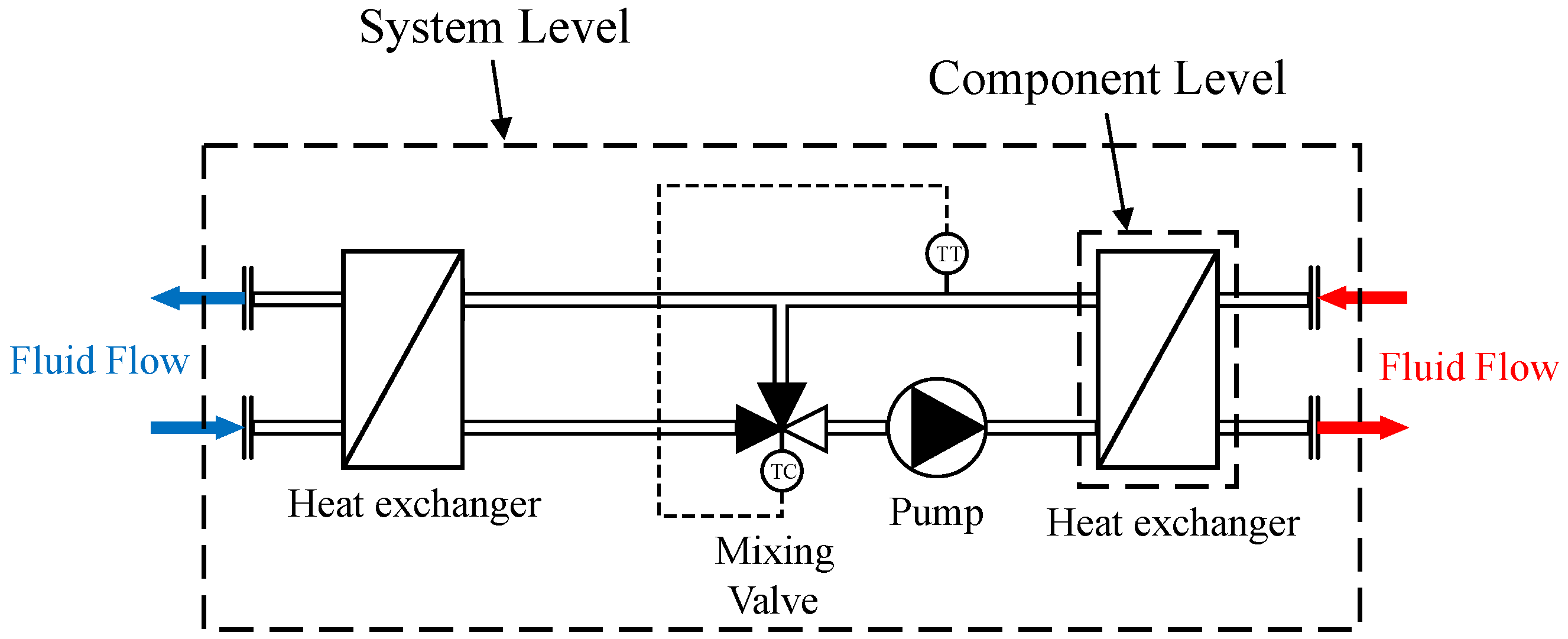
The proposed methodology uses these two views at different structural levels as shown in Figure 1. Computational causality is imposed on component interfaces to obtain executable component maps, whereas the coupling between components is retained in acausal form through junction balance equations. This separation is essential for the tearing reduction introduced below: causal component maps and locally solvable junction relations can be evaluated by forward propagation, while only the remaining algebraic loop variables are retained as tearing variables.

2.2. Component Interfaces: Externally Causal and Internally Implicit Models

A thermal–hydraulic network consists of components such as compressors, pumps, heat exchangers, valves, pipes, and separators. At steady state, each component interacts with the surrounding network only through its port variables, typically pressure p, specific enthalpy h, and mass flow rate $\dot{m}$. In the proposed methodology, components are exposed to the network assembly through externally causal interfaces, while their internal physics may remain implicit.

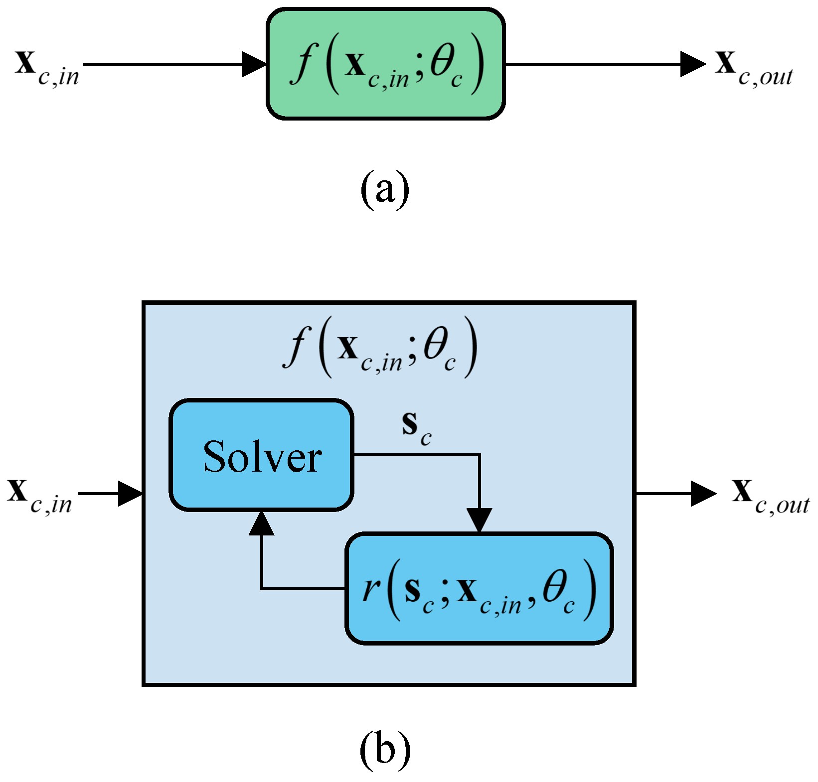
Let $x_c^{\mathrm{in}}\in {\mathbb{R}}^{n_c^{\mathrm{in}}}$ denote the input vector of component c, as defined by the assigned computational causality, and let $x_c^{\mathrm{out}}\in {\mathbb{R}}^{n_c^{\mathrm{out}}}$ denote the corresponding output vector. The component is interfaced to the network solver through an evaluation map

$$x_c^{\mathrm{out}}=f_c\left(x_c^{\mathrm{in}};{\theta }_c\right),$$

(1)

where ${\theta }_c$ denotes component parameters.

The map $f_c(·)$ defines the externally visible computational causality of the component. Once the required input port variables $x_c^{\mathrm{in}}$ are available, the component returns the corresponding output port variables $x_c^{\mathrm{out}}$. This externally causal interface is the object used by the network-level structural analysis and tearing algorithm.

Importantly, the existence of an externally causal interface does not imply that the component physics must be explicit. Many components are more naturally described by local implicit relations, for example, in residual form

$$r_c\left(s_c,x_c^{\mathrm{in}};{\theta }_c\right)=0,$$

(2)

where $s_c$ denotes component-internal states, such as segment pressures, enthalpies, or wall temperatures in a discretized heat-exchanger model. In this case, the evaluation of $f_c(x_c^{\mathrm{in}};{\theta }_c)$ involves solving the local system for $s_c$ and subsequently computing the output port variables.

This distinction is essential for the proposed reduction strategy. Component- internal states $s_c$ are not exposed as global network variables. The global network problem is formulated only in terms of port-level coupling variables, whereas component-local nonlinear systems are encapsulated within the corresponding component maps. Consequently, increasing the internal resolution of a component, for example, by using more heat-exchanger segments, does not necessarily increase the dimension of the global tearing problem. The nonlinear iterations at the network level are restricted to the coupling variables that remain after graph-based tearing.

Figure 2 illustrates this distinction for an externally causal component map and for a component whose external map contains an encapsulated local implicit solve.

2.3. Model Nonlinearities

The proposed methodology is not restricted to a particular degree of model nonlinearity. Component models may be linear, nonlinear, empirical, tabulated, or internally implicit, depending on the selected level of model fidelity. The only requirement at the network level is that each component provides an externally causal computational interface consistent with the assigned component causality.

The nonlinearities of the assembled residual system therefore originate from the selected component and property models, as well as from the thermal–hydraulic coupling equations, rather than from the causal–acausal formulation itself. In thermal–hydraulic applications, typical sources of nonlinearity include thermodynamic property evaluations, such as $T(p,h)$, $\rho (p,h)$, or saturation relations; component characteristic maps, such as compressor or valve correlations; heat transfer relations involving temperature differences; and pressure-flow relations in hydraulic components. In addition, junction energy balances introduce nonlinear coupling terms through the products of mass flow rate and specific enthalpy, whenever both quantities are unknown. In inverse and optimization problems, additional nonlinearities may enter through target functions, operational constraints, or actuator limits.

Consequently, the degree of nonlinearity is not a fixed property of the proposed methodology, but depends on how a thermal–hydraulic network is constructed within the framework. In particular, it is determined by the modeler’s choice of component models, property models, and coupling equations, provided that the selected models satisfy the externally causal interface requirements introduced above.

2.4. Computational Causality Types at Component Ports

To assemble and evaluate a network, each component is assigned a computational causality that specifies which port variables must be provided as inputs and which port variables are returned as outputs. This causality assignment is a computational interface convention, not a statement about the physical direction of cause and effect inside the component. It defines how the component can be executed during the forward reconstruction induced by the tearing algorithm.

In the present framework, each port is described by the variables pressure p, specific enthalpy h, and mass flow rate $\dot{m}$. Following [14], we distinguish two component causality types:

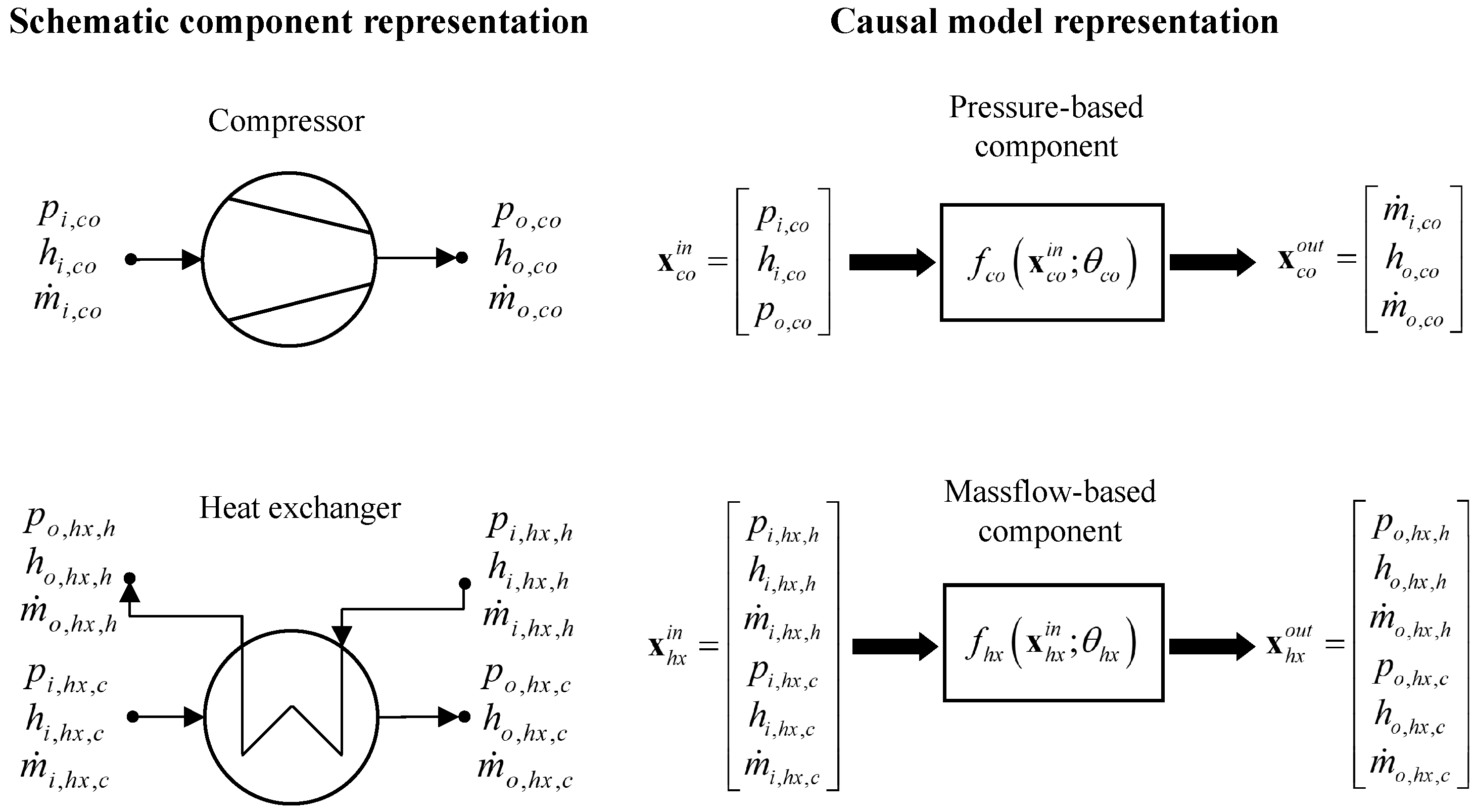
• Pressure-based components. These components take the pressures at the inlet and outlet ports, together with the inlet specific enthalpies, as inputs. They return the mass flow rates at all ports and the outlet specific enthalpies. Typical examples are compressors, pumps, and throttling or expansion devices, for which the mass flow rate is determined from pressure levels and component characteristics.
• Mass flow-based components. These components take pressure, specific enthalpy, and mass flow rate at the inlet ports as inputs and return the corresponding outlet port variables. Typical examples are heat exchangers, pipes, or other flow-through components that are evaluated along a prescribed flow direction.

These two causality types cover the component classes used in the present methodology: components whose mass flow rate is determined by pressure levels and components whose outlet state is evaluated along a known mass-flow direction. Once the required input variables of a component are available, the component becomes executable and its output variables can be propagated through the network. This executable structure is exploited by the graph-based tearing procedure described in Section 2.6.

The two causality types are summarized in

Table 1. Computational causality types used for component interfaces in the proposed methodology.

Causality Type	Inputs ${\mathbf{x}}_{\mathit{c}}^{\mathit{in}}$	Outputs ${\mathbf{x}}_{\mathit{c}}^{\mathit{out}}$
Pressure-based component	p, h at inlet ports p at outlet ports	$\dot{m}$ at all ports h at outlet ports
Mass-flow-based component	p, h, $\dot{m}$ at inlet ports	p, h, $\dot{m}$ at outlet ports

and illustrated in Figure 3 for a pressure-based compressor and a mass-flow-based heat exchanger.

2.5. Network Coupling: Junction Equations, Boundary Conditions, and Loop Closure

The system-level state of a thermal–hydraulic network is described by the port variables of all component connections. We collect the unknown pressures, specific enthalpies, and mass flow rates at component ports into the global network variable vector

$$\mathbf{x}\in {\mathbb{R}}^{n_x}.$$

(3)

The vector $\mathbf{x}$ contains only network coupling variables and no component-internal states. Quantities that are prescribed externally, such as boundary pressures, inlet enthalpies, inlet mass flow rates, actuator settings, and fixed component specifications, are collected in the input vector

$$\mathbf{u}\in {\mathbb{R}}^{n_u}.$$

(4)

Boundary conditions are therefore not introduced as additional residual equations. Instead, they determine which quantities are treated as prescribed inputs and which port variables remain unknowns in $\mathbf{x}$. This assignment follows from the combination of network topology and component causality: variables required by a component interface but not determined through junction coupling or by the output of another component must be supplied as external specifications. The residual equations of the network are then assembled for the remaining unknown port variables.

2.5.1. Junction Balance Equations

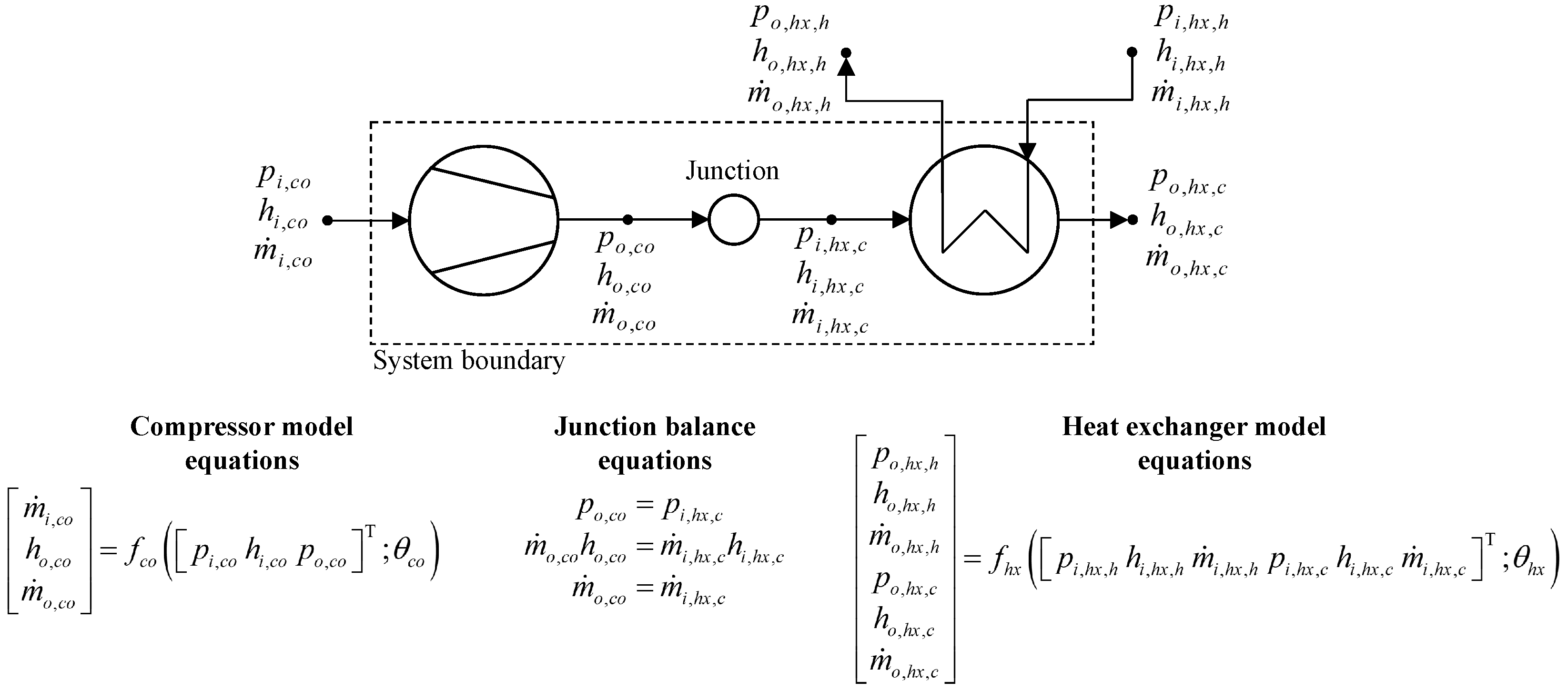
Components are interconnected through junctions. For each junction j, let ${\mathcal{P}}_j^{\mathrm{in}}$ denote the set of ports whose mass flow enters the junction and ${\mathcal{P}}_j^{\mathrm{out}}$ the set of ports whose mass flow leaves the junction. Mass flow rates are treated as non-negative with respect to the assigned port direction; the sets ${\mathcal{P}}_j^{\mathrm{in}}$ and ${\mathcal{P}}_j^{\mathrm{out}}$ therefore define the signs with which the corresponding streams enter the junction balances. Each connected port carries the variables $(p_{j,k},h_{j,k},{\dot{m}}_{j,k})$, which are either unknown entries of $\mathbf{x}$ or prescribed quantities contained in $\mathbf{u}$. An illustrative coupling of two component ports through a junction is shown in Figure 4.

At steady state, junctions neither store mass nor energy. The mass and energy balances are therefore given by

$$\sum _{k\in {\mathcal{P}}_j^{\mathrm{in}}}{\dot{m}}_{j,k}-\sum _{k\in {\mathcal{P}}_j^{\mathrm{out}}}{\dot{m}}_{j,k}=0,$$

(5)

$$\sum _{k\in {\mathcal{P}}_j^{\mathrm{in}}}{\dot{m}}_{j,k}{h}_{j,k}-\sum _{k\in {\mathcal{P}}_j^{\mathrm{out}}}{\dot{m}}_{j,k}{h}_{j,k}=0.$$

(6)

Pressure continuity is enforced by requiring all connected ports to share the same pressure. Choosing one connected port $k^{★}$ as reference, this can be written as

$$p_{j,k}-p_{j,k^{★}}=0,\forall k\in {\mathcal{P}}_j^{\mathrm{in}}\cup {\mathcal{P}}_j^{\mathrm{out}}.$$

(7)

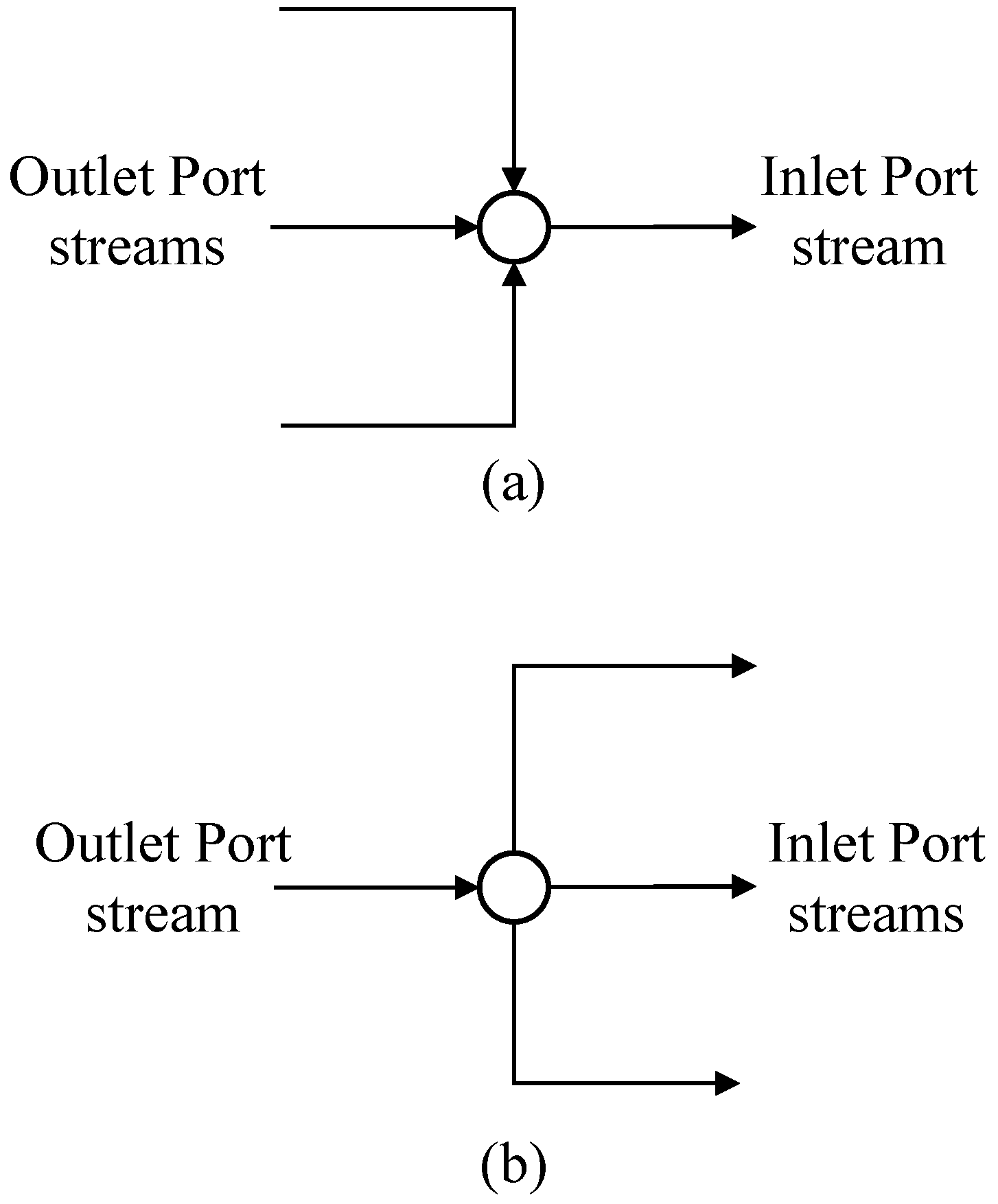
Two basic junction patterns are distinguished. A split junction connects one incoming stream to multiple outgoing streams. Since no mixing between different incoming streams occurs, all outgoing streams inherit the specific enthalpy of the incoming stream:

$$h_{j,k}-h_{j,k^{\mathrm{in}}}=0,\forall k\in {\mathcal{P}}_j^{\mathrm{out}},$$

(8)

where $k^{\mathrm{in}}$ denotes the unique incoming port.

A merge junction connects multiple incoming streams to one outgoing stream. In this case, perfect mixing is represented by the energy balance above; no equal-enthalpy constraints are imposed on the incoming streams. The outlet enthalpy is therefore determined implicitly by the mixed energy balance. The basic split and merge connection patterns are illustrated in Figure 5.

Collecting all junction balance and junction consistency equations yields the network coupling system of residual equations:

$${\mathcal{R}}_j(\mathbf{x};\mathbf{u})=\mathbf{0}.$$

(9)

Here, the dependence on $\mathbf{u}$ indicates that prescribed boundary values and fixed component inputs enter the residual evaluation as known quantities, whereas the remaining unknown port variables are collected in $\mathbf{x}$.

2.5.2. Boundary Conditions and Structural Well-Posedness

A well-posed steady-state network problem requires a structurally non-singular set of equations for the unknown network variables. In the proposed methodology, boundary conditions are assigned before the residual system is solved. They classify selected port variables, actuator settings, or model specifications as prescribed quantities and collect them in the input vector $\mathbf{u}$. The remaining unknown port variables form the network variable vector $\mathbf{x}$.

The need for boundary conditions follows from the combination of network topology and component causality. If a variable required by a component interface is not provided by junction coupling or by the output of another component, it must be prescribed externally. For example, an unconnected inlet of a mass-flow-based component requires pressure, specific enthalpy, and mass flow rate as boundary specifications. For a pressure-based component, pressures at the inlet and outlet ports and inlet specific enthalpies must be available as inputs to the component map, whereas the corresponding mass flow rates and outlet enthalpies are computed by the component model.

Thus, boundary conditions do not add independent balance equations to the network residual. Rather, they determine which quantities are known and which port variables remain unknown. This classification fixes the dimension of $\mathbf{x}$, determines the arguments of the component evaluation maps, and thereby defines the structure of the network coupling system of residuals ${\mathcal{R}}_j(\mathbf{x};\mathbf{u})=\mathbf{0}$.

2.5.3. Closed Loops and Additional Closure Relations

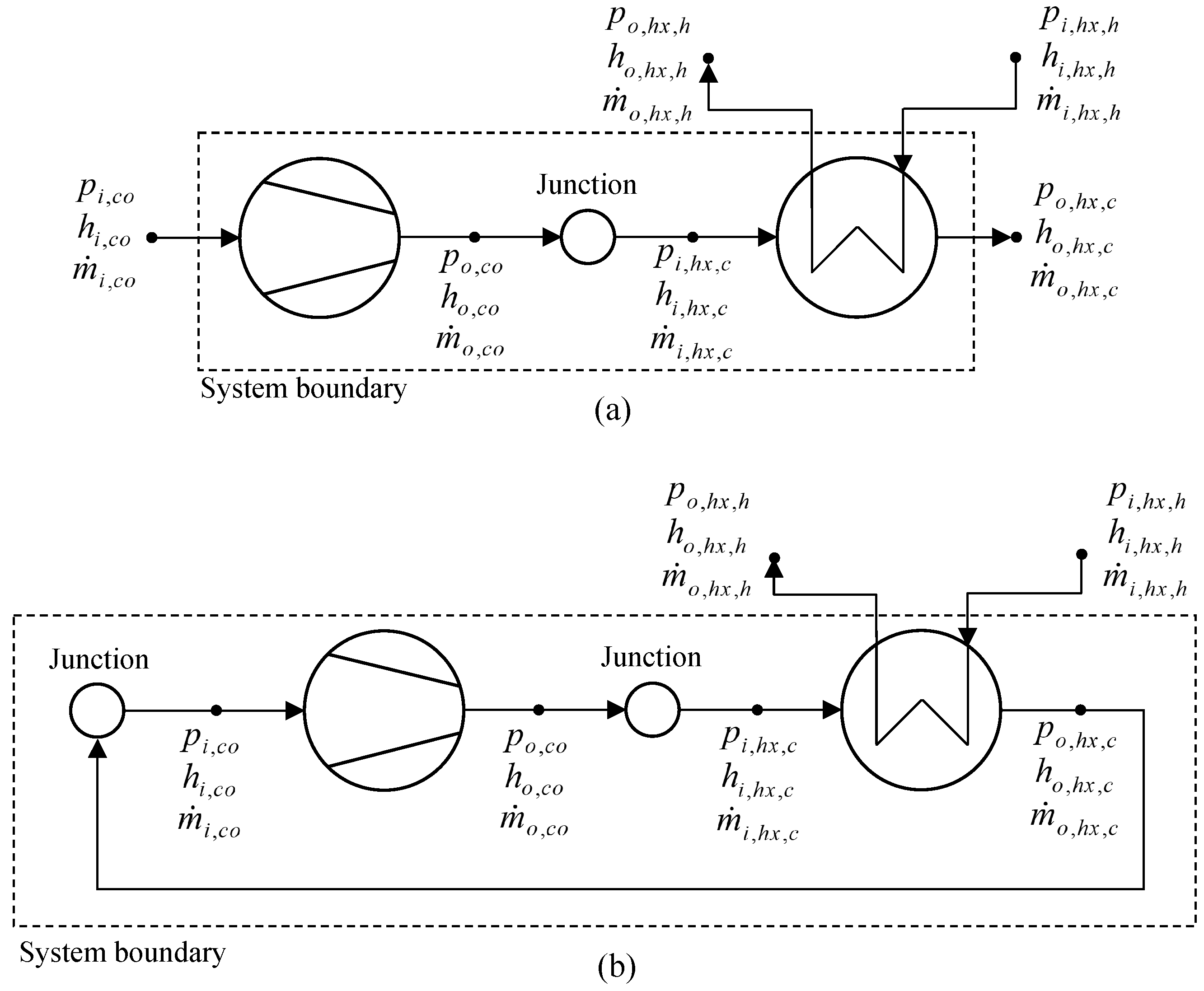
Network topology directly affects structural well-posedness. In particular, closed fluid loops may leave one or more degrees of freedom undetermined by junction balances and causally evaluated components alone. Figure 6 illustrates the difference between open- and closed-loop configurations.

The structural origin of this indeterminacy is that mass balance equations around a closed loop become linearly dependent. As a result, the junction balance equations and component evaluations are insufficient to determine all loop variables uniquely. In such cases, additional independent closure relations must be introduced. The number of required closure relations follows from the structural degrees of freedom of the assembled system; for the simple closed loops considered in this work, one additional independent closure relation is required per independent loop.

Unlike ordinary boundary conditions, which classify quantities as prescribed inputs in $\mathbf{u}$, closure relations are added as residual equations or equality constraints. They may encode physically meaningful specifications, such as fixing a pressure level, prescribing a thermodynamic state, imposing a receiver-state condition, fixing the total fluid inventory, or enforcing a device-specific steady-state assumption.

We denote the collection of closure relations in residual form by

$${\mathcal{R}}_c(\mathbf{x};\mathbf{u})=\mathbf{0}.$$

(10)

Together with the junction coupling residual, the structurally closed network problem is then written as

$$\tilde{\mathcal{R}}(\mathbf{x};\mathbf{u})=\left[\begin{array}{c}{\mathcal{R}}_j(\mathbf{x};\mathbf{u})\\ {\mathcal{R}}_c(\mathbf{x};\mathbf{u})\end{array}\right]=\mathbf{0}.$$

(11)

2.6. Tripartite-Graph-Based Tearing and Forward Reconstruction

After assigning component causalities, prescribing the required boundary conditions, and adding any necessary closure relations, the steady-state network problem is represented by the structurally closed residual system

$$\tilde{\mathcal{R}}(\mathbf{x};\mathbf{u})=\mathbf{0}.$$

(12)

Although component models are exposed through externally causal interfaces, the acausal junction balance equations can induce algebraic loops at the network level. Solving the full residual system directly may therefore become computationally expensive and numerically brittle, especially for large networks. To restrict nonlinear iterations to a reduced subset of variables, we apply tearing techniques [11,12,13]. The key idea is to identify a set of tearing variables that remain unknown in the nonlinear solve, while all remaining network variables are reconstructed by directed forward evaluation of executable component maps and solvable junction relations.

2.6.1. Tearing Algorithm

We adopt the tripartite-graph tearing algorithm of Huang et al. [14]. In the present framework, the tearing algorithm is used as a structural preprocessing step. Based on the assigned component causalities, the network junction equations, and any required closure relations, it determines (i) a causally admissible execution order of component evaluations and solvable junction relations, (ii) a set of tearing variables, and (iii) the residual equations that remain after forward evaluation.

The underlying principle is to exploit all causal relations that can be evaluated directly once their inputs are known. A component becomes executable as soon as all variables required by its computational causality are available. Likewise, a junction relation becomes solvable when all variables required to determine the remaining unknown are known. By successively marking variables as known and evaluating all executable components and solvable junction relations, the algorithm propagates information through the network as far as possible without iteration.

If no further forward evaluation is possible, additional tearing is introduced by selecting variables that remain temporarily undetermined and promoting them to tearing variables. These variables are retained as unknowns in the reduced network closure problem, while all remaining variables are determined by forward evaluation. The tearing procedure induces a partition of the unknown network variables,

$$\mathbf{x}={\mathbf{P}}^{\top }\left[\begin{array}{c}\mathbf{z}\\ \mathbf{w}\end{array}\right],$$

(13)

where $\mathbf{z}\in {\mathbb{R}}^{n_z}$ denotes the vector of tearing variables, $\mathbf{w}\in {\mathbb{R}}^{n_x-n_z}$ collects all remaining non-tearing port variables, and $\mathbf{P}$ is a permutation matrix that maps the ordered partition back to the original ordering of $\mathbf{x}$. By construction of the execution order, $\mathbf{w}$ can be reconstructed by a single forward pass once $(\mathbf{z};\mathbf{u})$ is given.

The residual equations are formed by those balance relations that are not eliminated through forward propagation and therefore close the remaining algebraic loop. Collecting these residuals defines a compact nonlinear system, referred to as the tearing-reduced residual system:

$${\mathcal{R}}_t(\mathbf{z};\mathbf{u})=\mathbf{0},$$

(14)

where the subscript t denotes tearing-reduced. In typical applications, the reduced dimension d is much smaller than $n_x$, which reduces the cost of nonlinear iterations. The tearing procedure does not alter the underlying physical model. Rather, it reorganizes the algebraic structure of the network equations such that only a reduced subset of variables remains in the nonlinear solve, while the remaining variables are recovered by directed forward evaluation.

Accordingly, the structural reduction achieved by tearing is governed by the number and arrangement of algebraic couplings that cannot be resolved by forward evaluation. Networks for which only a comparatively small set of tearing variables remains therefore lead to a correspondingly compact network-level nonlinear residual system. The resulting computational benefit, however, also depends on the cost of evaluating the selected component and property models.

2.6.2. Forward Reconstruction Operator

In addition to the tearing variables and residual equations, the tearing algorithm provides a causally admissible execution order for component evaluations and solvable junction relations. This execution order induces a deterministic forward reconstruction operator

$$\mathbf{w}=\psi (\mathbf{z};\mathbf{u}),$$

(15)

which reconstructs all non-tearing port variables from the tearing variables and prescribed inputs. Component-internal solves, if present, are encapsulated within the component maps $f_c(·)$ and therefore do not introduce additional global unknowns.

The complete network port-variable state implied by $(\mathbf{z};\mathbf{u})$ is then given by

$$\mathbf{x}(\mathbf{z};\mathbf{u})={\mathbf{P}}^{\top }\left[\begin{array}{c}\mathbf{z}\\ \psi (\mathbf{z};\mathbf{u})\end{array}\right].$$

(16)

For notational simplicity, $\mathbf{P}$ may be omitted when the network variables are ordered such that the tearing variables appear first.

The tearing-reduced residual system can therefore be viewed as a reduced representation of the structurally closed steady-state network problem $\tilde{\mathcal{R}}(\mathbf{x};\mathbf{u})=\mathbf{0}$. Formally, the reduced residual is obtained by evaluating the remaining residual equations after forward reconstruction:

$${\mathcal{R}}_t(\mathbf{z};\mathbf{u})={\mathbf{S}}^{\top }\tilde{\mathcal{R}}\left(\mathbf{x}(\mathbf{z};\mathbf{u});\mathbf{u}\right),$$

(17)

where $\mathbf{S}$ denotes the selection operator of residual equations that remain after tearing and forward propagation.

In summary, the proposed methodology transforms the structurally closed steady-state network problem $\tilde{\mathcal{R}}(\mathbf{x};\mathbf{u})=\mathbf{0}$ into a tearing-reduced formulation in terms of $\mathbf{z}$, together with a forward reconstruction operator $\psi (\mathbf{z};\mathbf{u})$. This reduced representation provides the common mathematical basis for both direct simulation and tearing-reduced residual-constrained inverse or optimization problems.

2.7. Problem Formulations: Direct and Inverse Problems

The tearing reduction yields a compact nonlinear residual system ${\mathcal{R}}_t(\mathbf{z};\mathbf{u})=\mathbf{0}$ and a forward reconstruction operator $\psi (\mathbf{z};\mathbf{u})$. Together, they define the reconstructed network state $\mathbf{x}(\mathbf{z};\mathbf{u})$. This common representation enables different computational workflows without changing the underlying network model.

In addition to port variables, many tasks require system output quantities such as cooling load, superheat, compressor power, pressure levels, or efficiency. We therefore define a vector of system outputs as

$$\mathbf{y}=g\left(\mathbf{x}(\mathbf{z};\mathbf{u});\mathbf{u}\right),$$

(18)

where $g(·)$ is a post-processing map evaluated from the reconstructed steady-state solution and prescribed inputs.

2.7.1. Direct Problem (Steady-State Simulation)

In the direct problem, all external inputs are prescribed. These include boundary conditions, actuator settings, and fixed component specifications collected in $\mathbf{u}$. The unknowns of the reduced nonlinear problem are therefore only the tearing variables $\mathbf{z}$. The steady-state solution is obtained by solving

$${\mathcal{R}}_t(\mathbf{z};\mathbf{u})=\mathbf{0}$$

(19)

for $\mathbf{z}$ using a nonlinear root-finding method [8,9].

Once a solution ${\mathbf{z}}^{*}$ is obtained, the non-tearing variables, the full port-variable state, and the system outputs follow from

$${\mathbf{w}}^{*}=\psi ({\mathbf{z}}^{*};\mathbf{u}),{\mathbf{x}}^{*}=\mathbf{x}({\mathbf{z}}^{*};\mathbf{u}),{\mathbf{y}}^{*}=g({\mathbf{x}}^{*};\mathbf{u}).$$

(20)

2.7.2. Residual-Constrained Inverse and Optimization Problems

Inverse and optimization problems for steady-state networks can be expressed as residual-constrained optimization problems. Inverse problems in steady-state modeling arise naturally in design, parameter identification, and set-point tracking applications [28,29]. In equation-oriented environments such as TESPy, inverse tasks can often be addressed very naturally by changing which quantities are prescribed and which are solved for within the same steady-state model [5,30]. TESPy also supports the use of component parameters as variables and provides design/off-design switching mechanisms for adapting model specifications accordingly [30,31]. For many applications, this offers a flexible and elegant way to formulate alternative operating or design problems within a common network model.

In the present work, inverse problems are formulated explicitly in a simultaneous analysis and design setting on the tearing-reduced system. The key difference is that the tearing variables and selected variable inputs are treated as unknowns simultaneously, while the steady-state balance equations are enforced directly as constraints of the optimization problem. By contrast, when external optimization tools are coupled to a steady-state network model, the resulting workflow is typically nested, in the sense that the optimizer updates the decision variables and the network model is solved repeatedly for each new candidate point [32]. The simultaneous formulation adopted here is particularly attractive when the solution of the direct problem is itself computationally expensive or numerically challenging, as discussed in the Introduction.

The inverse problem is then formulated as a tearing-reduced residual-constrained optimization problem. The input vector is partitioned into variable and fixed inputs according to

$$\mathbf{u}=\left[\begin{array}{c}{\mathbf{u}}^{var}\\ {\mathbf{u}}^{fix}\end{array}\right],$$

(21)

where ${\mathbf{u}}^{var}$ contains selected variable inputs, such as actuator settings, boundary values, and design parameters, and ${\mathbf{u}}^{fix}$ contains the prescribed inputs that remain fixed during the optimization. For any candidate pair $(\mathbf{z},{\mathbf{u}}^{var})$, the full port-variable state is obtained from the forward reconstruction operator,

$$\mathbf{x}(\mathbf{z};\mathbf{u})={\mathbf{P}}^{\top }\left[\begin{array}{c}\mathbf{z}\\ \psi (\mathbf{z};\mathbf{u})\end{array}\right].$$

(22)

The resulting optimization problem is written as

$$\begin{array}{cc}\hfill \underset{\mathbf{z},{\mathbf{u}}^{var}}{min}& \mathcal{J}\left(\mathbf{x}(\mathbf{z};\mathbf{u}),{\mathbf{u}}^{var};{\mathbf{u}}^{fix}\right)\hfill \\ \hfill \mathrm{s}.\mathrm{t}.& {\mathcal{R}}_t\left(\mathbf{z};{\mathbf{u}}^{var},{\mathbf{u}}^{fix}\right)=\mathbf{0},\hfill \\ \hfill & \mathcal{H}\left(\mathbf{x}(\mathbf{z};\mathbf{u}),{\mathbf{u}}^{var};{\mathbf{u}}^{fix}\right)=\mathbf{0},\hfill \\ \hfill & \mathcal{G}\left(\mathbf{x}(\mathbf{z};\mathbf{u}),{\mathbf{u}}^{var};{\mathbf{u}}^{fix}\right)\le \mathbf{0},\hfill \\ \hfill & \underline{\mathbf{z}}\le \mathbf{z}\le \overline{\mathbf{z}},\hfill \\ \hfill & {\underline{\mathbf{u}}}^{var}\le {\mathbf{u}}^{\mathrm{var}}\le {\overline{\mathbf{u}}}^{var}.\hfill \end{array}$$

(23)

Here, ${\mathcal{R}}_t(·)$ denotes the tearing-reduced residual system and enforces steady-state feasibility of the reconstructed network state. The objective function $\mathcal{J}(·)$ represents either a set-point tracking objective or a performance metric evaluated from the reconstructed state and the variable inputs. The functions $\mathcal{H}(·)$ and $\mathcal{G}(·)$ encode additional equality and inequality constraints beyond steady-state feasibility, such as operational requirements, design specifications, or physical admissibility conditions. The bound constraints restrict the tearing variables and variable inputs to admissible ranges, for example, to represent actuator limits or physically meaningful operating domains.

This formulation is a tearing-reduced SAND formulation: the tearing variables $\mathbf{z}$ and selected variable inputs ${\mathbf{u}}^{var}$ are determined simultaneously, while all remaining network variables are obtained by forward reconstruction. Direct simulation, inverse problems, and more general optimization tasks are therefore expressed within the same tearing-reduced modeling framework. They differ only in the role assigned to selected entries of the input vector and in the choice of objective function and additional constraints.

The formulation in Equation (23) should be interpreted as a general nonlinear programming problem. In the general thermal–hydraulic case, global optimality guarantees cannot be stated without additional restrictive assumptions. Such guarantees are available only for special cases, for example, when the residual equality constraints are affine, the inequality constraints define a convex feasible set, the objective function is convex, and suitable regularity and feasibility conditions hold.

As discussed in Section 2.3, thermal–hydraulic inverse problems generally involve nonlinear component, property, and coupling relations. Consequently, the residual-constrained inverse problems considered in this work are generally nonconvex. Solutions obtained with nonlinear programming solvers should therefore be interpreted as locally optimal or stationary solutions, depending on the solver, initialization, and constraint regularity, rather than as globally optimal solutions in the general case.

3. Test Case

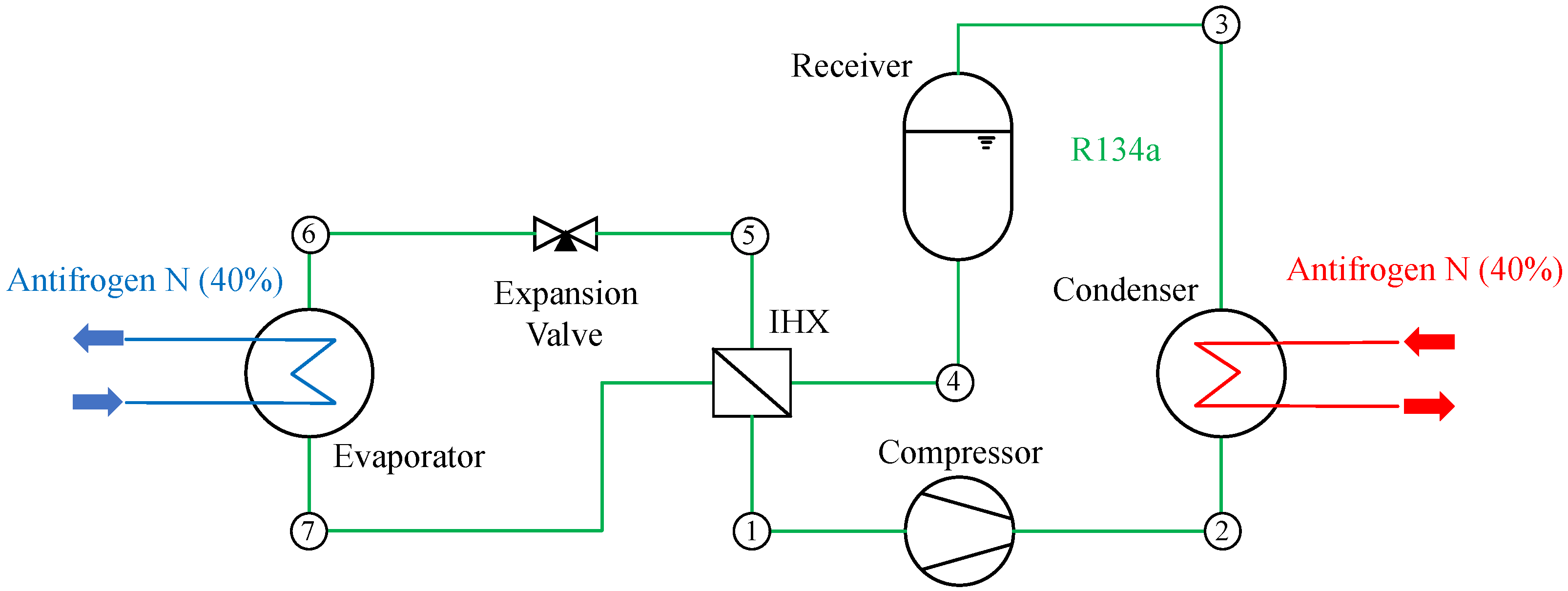
The proposed modeling methodology is now demonstrated on a test case involving a vapor-compression refrigeration cycle using R134a as the refrigerant. Antifrogen N at 40% concentration serves as the cooling and heating media. The cycle comprises a compressor, evaporator, condenser, receiver, internal heat exchanger (IHX), and an electronic expansion valve, as shown in Figure 7. In the following, the numerical models used for each component, as well as the system-level equations, are explained.

3.1. Compressor Modeling

A variable-speed reciprocating compressor is modeled as a pressure-based component, with its numerical model derived from steady-state data provided by the compressor manufacturer [33]. The model describes compressor performance using efficiency maps [34]. The refrigerant mass flow rate is calculated by

$${\dot{m}}_i={\dot{m}}_o={\rho }_i·{\eta }_v·V_d·\omega ,$$

(24)

where ${\rho }_i$ is the refrigerant density at the inlet port, $V_d$ is the fixed compressor displacement, and $\omega$ is the compressor rotational speed. The volumetric efficiency, ${\eta }_v$, is correlated using a polynomial function of the pressure ratio and compressor speed,

$${\eta }_v=a_0·\left({\displaystyle \frac{p_o}{p_i}}\right)+a_1·{\left({\displaystyle \frac{p_o}{p_i}}\right)}^2+a_2·\omega +a_3,$$

(25)

where $a_0$ to $a_3$ are constant coefficients. The power consumption is estimated based on the isentropic efficiency ${\eta }_{is}$,

$${\eta }_{is}={\displaystyle \frac{{\dot{m}}_i·\left(h_{o,\mathrm{is}}-h_i\right)}{\dot{W}}},$$

(26)

which is fitted as follows:

$${\eta }_{is}=b_0·\left({\displaystyle \frac{p_o}{p_i}}\right)+b_1·{\left({\displaystyle \frac{p_o}{p_i}}\right)}^2+b_2·\omega +b_3·\omega ·\left({\displaystyle \frac{p_o}{p_i}}\right)+b_4.$$

(27)

The refrigerant discharge state is determined by applying an energy balance to the compressor:

$$\dot{W}={\dot{m}}_i·\left(h_o-h_i\right),$$

(28)

assuming heat losses are negligible.

3.2. Evaporator and Condenser Modeling

The evaporator and condenser are modeled as mass-flow-based components using a finite-difference discretization. Assuming one-dimensional steady-state flow along the axial coordinate $x\in [0,L]$, constant cross-sectional areas for both fluids, and negligible frictional pressure losses, the mass, momentum, and energy balance equations can be written as

$${\displaystyle \frac{\partial {\dot{m}}_h}{\partial x}}=0\Rightarrow {\dot{m}}_h=\mathrm{const},$$

(29)

$${\displaystyle \frac{\partial {\dot{m}}_c}{\partial x}}=0\Rightarrow {\dot{m}}_c=\mathrm{const},$$

(30)

$${\displaystyle \frac{\partial p_h}{\partial x}}=0\Rightarrow p_h=\mathrm{const},$$

(31)

$${\displaystyle \frac{\partial p_c}{\partial x}}=0\Rightarrow p_c=\mathrm{const},$$

(32)

$${\displaystyle \frac{\partial h_h}{\partial x}}=-{\displaystyle \frac{U·A}{{\dot{m}}_h·L}}·(T_h-T_c),$$

(33)

$${\displaystyle \frac{\partial h_c}{\partial x}}={\displaystyle \frac{U·A}{{\dot{m}}_c·L}}·(T_h-T_c),$$

(34)

where the subscripts h and c denote the hot and cold sides of the heat exchanger, respectively, U is the overall heat transfer coefficient, A is the total heat transfer area, and L is the total heat-exchange length.

Additionally, the boundary conditions for a counterflow heat-exchanger arrangement are defined as follows:

$$h_c\left(0\right)=h_{i,c},$$

(35)

$$h_h\left(L\right)=h_{i,h}.$$

(36)

From the mass balance, it follows that

$${\dot{m}}_c\left(x\right)={\dot{m}}_{i,c},\forall x\in [0,L]\Rightarrow {\dot{m}}_{o,c}={\dot{m}}_{i,c},$$

(37)

$${\dot{m}}_h\left(x\right)={\dot{m}}_{i,h},\forall x\in [0,L]\Rightarrow {\dot{m}}_{o,h}={\dot{m}}_{i,h}.$$

(38)

From the momentum balance, the following conditions apply:

$$p_c\left(x\right)=p_{i,c},\forall x\in [0,L]\Rightarrow p_{o,c}=p_{i,c},$$

(39)

$$p_h\left(x\right)=p_{i,h},\forall x\in [0,L]\Rightarrow p_{o,h}=p_{i,h}.$$

(40)

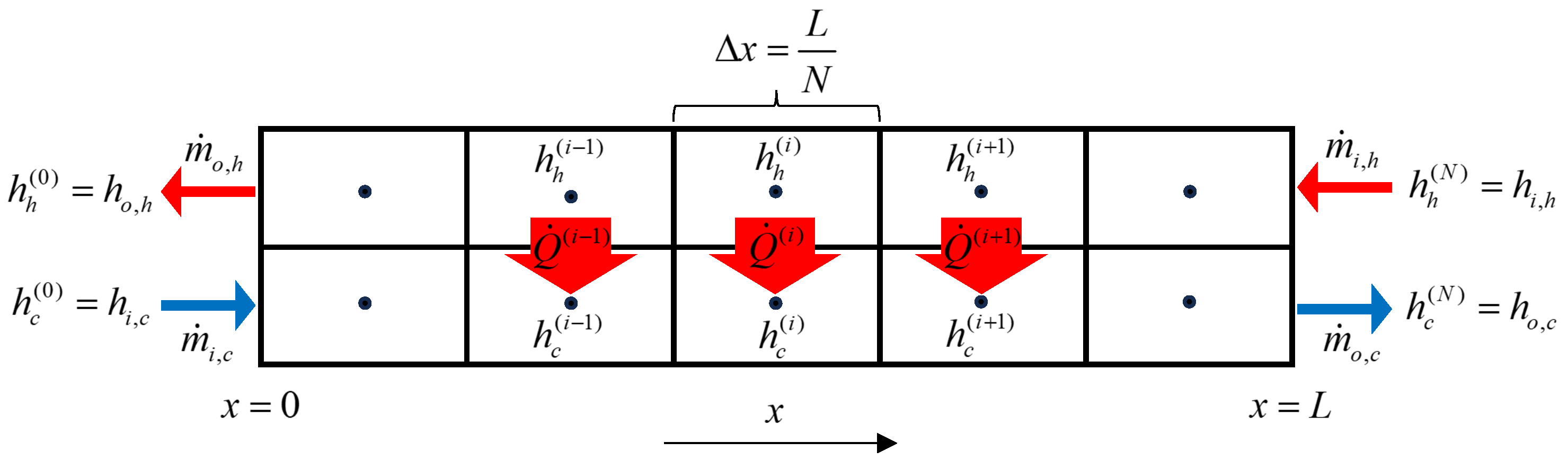
The partial differential equations for the energy balance are then discretized using a finite-difference method. The heat exchanger is divided into N segments along the length L, with each segment having a length of $\Delta x={\displaystyle \frac{L}{N}}$, as shown in Figure 8. The discretization of the energy balance equations leads to

$$h_c^{(i+1)}=h_c^{\left(i\right)}+{\displaystyle \frac{U·A·\Delta x}{{\dot{m}}_c·L}}·(T_h^{\left(i\right)}-T_c^{\left(i\right)}),\forall i=1,2,\dots ,N,$$

(41)

$$h_h^{(i+1)}=h_h^{\left(i\right)}-{\displaystyle \frac{U·A·\Delta x}{{\dot{m}}_h·L}}·(T_h^{\left(i\right)}-T_c^{\left(i\right)}),\forall i=1,2,\dots ,N,$$

(42)

with the discretized boundary conditions

$$h_c^{(i=0)}=h_{i,c},$$

(43)

$$h_h^{(i=N)}=h_{i,h}.$$

(44)

It follows that the outlet specific enthalpies for the hot- and cold-side fluids are then given by

$$h_{o,c}=h_c^{\left(N\right)},$$

(45)

$$h_{o,h}=h_h^{\left(0\right)}.$$

(46)

Because of the counterflow arrangement, the boundary conditions for the enthalpies of the hot and cold fluids are specified at different locations within the discretized domain. Consequently, this creates a boundary-value problem (BVP), which can be solved using the shooting method [35] for an effective solution.

3.3. Internal Heat-Exchanger Modeling

The internal heat exchanger (IHX) was also modeled as a mass-flow-based component but modeled using the $ϵ$-NTU method [36]. In the $ϵ$-NTU method, the number of transfer units (NTU) is defined by

$$NTU={\displaystyle \frac{U·A}{max({\dot{C}}_h,{\dot{C}}_c)}},$$

(47)

where A is the total heat transfer area of the heat exchanger, U the overall heat transfer coefficient, and ${\dot{C}}_h=c_p{\dot{m}}_h$ and ${\dot{C}}_c=c_p{\dot{m}}_c$ represent the capacity rates of the hot and cold fluids, respectively. Furthermore, the thermal efficiency of the heat exchanger is defined by

$$ϵ={\displaystyle \frac{T_{i,h}-T_{o,h}}{T_{i,h}-T_{i,c}}}={\displaystyle \frac{\dot{Q}/{\dot{C}}_h}{T_{i,h}-T_{i,c}}}.$$

(48)

For a counter-current heat exchanger, the thermal efficiency can be calculated as a function of the NTU and capacity rates ${\dot{C}}_c$ and ${\dot{C}}_h$ by

$$ϵ={\displaystyle \frac{1-e^{-NTU·(1-{\dot{C}}_h/{\dot{C}}_c)}}{1-{\dot{C}}_h/{\dot{C}}_c·e^{-NTU·\left(1-{\dot{C}}_h/{\dot{C}}_c\right)}}}.$$

(49)

Combining equations (Equation (47)) through (Equation (49)) enables the calculation of the heat transfer rate $\dot{Q}$, which then facilitates the calculation of the outlet specific enthalpies through

$$h_{o,h}=h_{i,h}-{\displaystyle \frac{\dot{Q}}{{\dot{m}}_{i,h}}}$$

(50)

$$h_{o,c}=h_{i,c}+{\displaystyle \frac{\dot{Q}}{{\dot{m}}_{i,c}}}.$$

(51)

Pressure losses in all heat exchangers were neglected. Thus, for the pressure values at the inlet and outlet ports, the following equations hold:

$$p_{i,h}=p_{o,h},$$

(52)

$$p_{i,c}=p_{o,c}.$$

(53)

3.4. Expansion Valve Modeling

The electronic expansion valve is modeled as a pressure-based component, with the mass flow rates at the inlet and outlet given by

$${\dot{m}}_i={\dot{m}}_o=C_f·A_v·\sqrt{{\rho }_i·(p_i-p_o)},$$

(54)

where $A_v$ is the adjustable normalized valve opening area used to control superheat at the evaporator outlet, and $C_f$ is a constant expansion valve flow coefficient. Additionally, isenthalpic expansion is assumed:

$$h_o=h_i.$$

(55)

3.5. Receiver Modeling

The receiver in a refrigeration system collects refrigerant and separates vapor from liquid. At steady state, the refrigerant exiting the receiver is in a saturated-liquid state. Assuming no heat or pressure losses, the refrigerant’s condition depends solely on the receiver pressure level. The following equations apply:

$$h_o=h_s\left(p_i\right)$$

(56)

$${\dot{m}}_o={\dot{m}}_i$$

(57)

$$p_o=p_i,$$

(58)

where $h_s\left(p_i\right)$ is the specific enthalpy at saturation liquid state at the pressure level of the receiver.

3.6. System-Level Equations

Applying the tearing algorithm to the vapor-compression refrigeration cycle, modeled using the numerical component models described above, reduces the steady-state network problem from $n_x=54$ coupled port variables to a reduced nonlinear system with $d=6$ tearing variables. All remaining non-tearing port variables are either reconstructed through a single forward evaluation $\psi (·)$ induced by the causally admissible execution order or prescribed via boundary conditions. The resulting tearing-variable vector is

$$\mathbf{z}={\left[\begin{array}{cccccc}{p}_{i,\mathrm{co}}& h_{i,\mathrm{co}}& p_{o,\mathrm{co}}& p_{i,\exp }& h_{i,\exp }& p_{o,\exp }\end{array}\right]}^{\top }.$$

The corresponding residual equations of the torn system are given by

$${\mathcal{R}}_t\left(\mathbf{z};\mathbf{u}\right)=\mathbf{0}\iff \left\{\begin{array}{cc}\hfill p_{i,\mathrm{co}}-p_{o,\mathrm{ihx},\mathrm{c}}(\mathbf{z};\mathbf{u})& =0,\hfill \\ \hfill h_{i,\mathrm{co}}-h_{o,\mathrm{ihx},\mathrm{c}}(\mathbf{z};\mathbf{u})& =0,\hfill \\ \hfill p_{i,\exp }-p_{o,\mathrm{ihx},\mathrm{h}}(\mathbf{z};\mathbf{u})& =0,\hfill \\ \hfill h_{i,\exp }-h_{o,\mathrm{ihx},\mathrm{h}}(\mathbf{z};\mathbf{u})& =0,\hfill \\ \hfill {\dot{m}}_{i,\exp }(\mathbf{z};\mathbf{u})-{\dot{m}}_{o,\mathrm{ihx},\mathrm{h}}(\mathbf{z};\mathbf{u})& =0,\hfill \end{array}\right.$$

(59)

where the subscripts i and o denote inlet and outlet ports, respectively, and the component labels $\mathrm{co}$, $\exp$, and $\mathrm{ihx}$ refer to the compressor, expansion valve, and internal heat exchanger, respectively. For the IHX, the additional subscripts $\mathrm{c}$ and $\mathrm{h}$ denote the cold and hot sides of the heat exchanger, respectively.

Thus, only five residual relations remain to be satisfied by the six tearing variables. This indicates one remaining degree of freedom that is not fixed by the junction balances and the selected component causalities alone. In this cycle configuration, the missing closure corresponds to the closed refrigerant loop and must be provided by an additional physically meaningful specification.

To close the system, consistency with the receiver model is enforced. At steady state, the receiver is assumed to deliver saturated liquid; thus, the receiver outlet enthalpy depends only on its pressure level:

$$h_{o,\mathrm{rev}}=h_s\left(p_{\mathrm{rev}}\right),p_{\mathrm{rev}}=p_{i,\mathrm{rev}}=p_{o,\mathrm{rev}}.$$

(60)

From the junction between the condenser outlet and the receiver inlet, we obtain

$$h_{i,\mathrm{rev}}=h_{o,\mathrm{r},\mathrm{cond}}.$$

(61)

Consistency with the saturated-liquid receiver assumption therefore requires the condenser outlet enthalpy to match the saturated-liquid enthalpy at the receiver pressure. This yields the additional closure relation

$$h_{o,\mathrm{r},\mathrm{cond}}-h_s\left(p_{o,\mathrm{r},\mathrm{cond}}\right)=0.$$

(62)

Incorporating Equation (62) together with the tearing residual system (59) yields a closed reduced formulation with six equations and six tearing variables.

4. Results

The test case introduced in Section 3 is now used to demonstrate the proposed methodology for both direct and inverse problem formulations. In all simulations, the condenser antifrogen inlet port temperature $T_{i,\mathrm{af},\mathrm{cond}}$ is varied across three operating points, namely, 16 °C, 24 °C, and 32 °C. All remaining antifrogen-side boundary conditions, including the evaporator inlet temperature $T_{i,\mathrm{af},\mathrm{evap}}$, the inlet pressures $p_{i,\mathrm{af},\mathrm{evap}}$ and $p_{i,\mathrm{af},\mathrm{cond}}$, and the inlet mass flow rates ${\dot{m}}_{i,\mathrm{af},\mathrm{evap}}$ and ${\dot{m}}_{i,\mathrm{af},\mathrm{cond}}$, are kept constant.

Two operating scenarios are considered. First, a direct problem is solved, representing a pure steady-state system simulation with all inputs prescribed. Second, an inverse problem is formulated in which the refrigerant superheat at the evaporator outlet and the evaporator cooling load are regulated to prescribed set-point values. Both scenarios are solved using the same steady-state network equations and tearing structure; only the role of selected system inputs differs.

Table 2. Summary of boundary conditions, model parameters, and decision variables used in the direct and inverse problem formulations.

Quantity	Symbol	Unit	Direct Problem (Simulation)	Inverse Problem (Set-Point Tracking)
Boundary conditions
Condenser inlet temperature	$T_{i,\mathrm{af},\mathrm{cond}}$	°C	16 / 24 / 32
Antifrogen evaporator inlet temperature	$T_{i,\mathrm{af},\mathrm{evap}}$	°C	0.0
Antifrogen evaporator inlet pressure	$p_{i,\mathrm{af},\mathrm{evap}}$	bar	1.0
Antifrogen evaporator inlet mass flow rate	${\dot{m}}_{i,\mathrm{af},\mathrm{evap}}$	$\mathrm{kg} {\mathrm{s}}^{-1}$	1.0
Antifrogen condenser inlet pressure	$p_{i,\mathrm{af},\mathrm{cond}}$	bar	1.0
Antifrogen condenser inlet mass flow rate	${\dot{m}}_{i,\mathrm{af},\mathrm{cond}}$	$\mathrm{kg} {\mathrm{s}}^{-1}$	1.0
Model parameters
Condenser heat transfer area	$A_{\mathrm{cond}}$	${\mathrm{m}}^2$	3.65
Evaporator heat transfer area	$A_{\mathrm{evap}}$	${\mathrm{m}}^2$	2.56
Internal heat-exchanger area	$A_{\mathrm{ihx}}$	${\mathrm{m}}^2$	0.50
Condenser overall heat transfer coefficient	$U_{\mathrm{cond}}$	$\mathrm{W} {\mathrm{m}}^{-2} {\mathrm{K}}^{-1}$	1000
Evaporator overall heat transfer coefficient	$U_{\mathrm{evap}}$	$\mathrm{W} {\mathrm{m}}^{-2} {\mathrm{K}}^{-1}$	1000
Internal heat-exchanger coefficient	$U_{\mathrm{ihx}}$	$\mathrm{W} {\mathrm{m}}^{-2} {\mathrm{K}}^{-1}$	1000
Expansion valve flow coefficient	$C_f$	${\mathrm{m}}^2$	0.25
Compressor displacement volume	$V_d$	${\mathrm{m}}^3$	0.00475
Model outputs
Evaporator cooling load	${\dot{Q}}_{\mathrm{evap}}$	$\mathrm{k}\mathrm{W}$	Free model response	Set-point target:= 15
Evaporator superheat	$\Delta T_{\mathrm{sh}}$	$\mathrm{K}$	Free model response	Set-point target:= 5
Actuation/decision variables
Normalized valve opening	$A_v$	–	0.4	Optimized $\in [0,1]$
Compressor speed	$\omega$	${\min }^{-1}$	1500	Optimized $\in [750,3500]$

summarizes all the boundary conditions, model parameters, and decision variables used in the test case. While the normalized expansion valve opening $A_v$ and the compressor rotational speed $\omega$ are fixed in the direct problem, they are treated as decision variables within prescribed bounds in the inverse problem formulation.

4.1. Direct Problem: Steady-State System Simulation

In the direct problem, the system is simulated for varying condenser antifrogen inlet temperatures $T_{i,\mathrm{af},\mathrm{cond}}$, while all remaining inputs are held constant. The corresponding system input vector is given by

$$\mathbf{u}={\left[\begin{array}{cccccccc}\omega & A_v& p_{i,\mathrm{af},\mathrm{cond}}& h_{i,\mathrm{af},\mathrm{cond}}& {\dot{m}}_{i,\mathrm{af},\mathrm{cond}}& p_{i,\mathrm{af},\mathrm{evap}}& h_{i,\mathrm{af},\mathrm{evap}}& {\dot{m}}_{i,\mathrm{af},\mathrm{evap}}\end{array}\right]}^{\top }.$$

In this scenario, only the antifrogen inlet enthalpy $h_{i,\mathrm{af},\mathrm{cond}}$ varies, as it depends on the specified condenser inlet temperature and pressure.

The direct problem is solved by applying a root-finding solver to the assembled system of steady-state residuals, Equation (59), together with the additional constraint (62). This yields a unique steady-state solution for all pressures, mass flow rates, and specific enthalpies in the network.

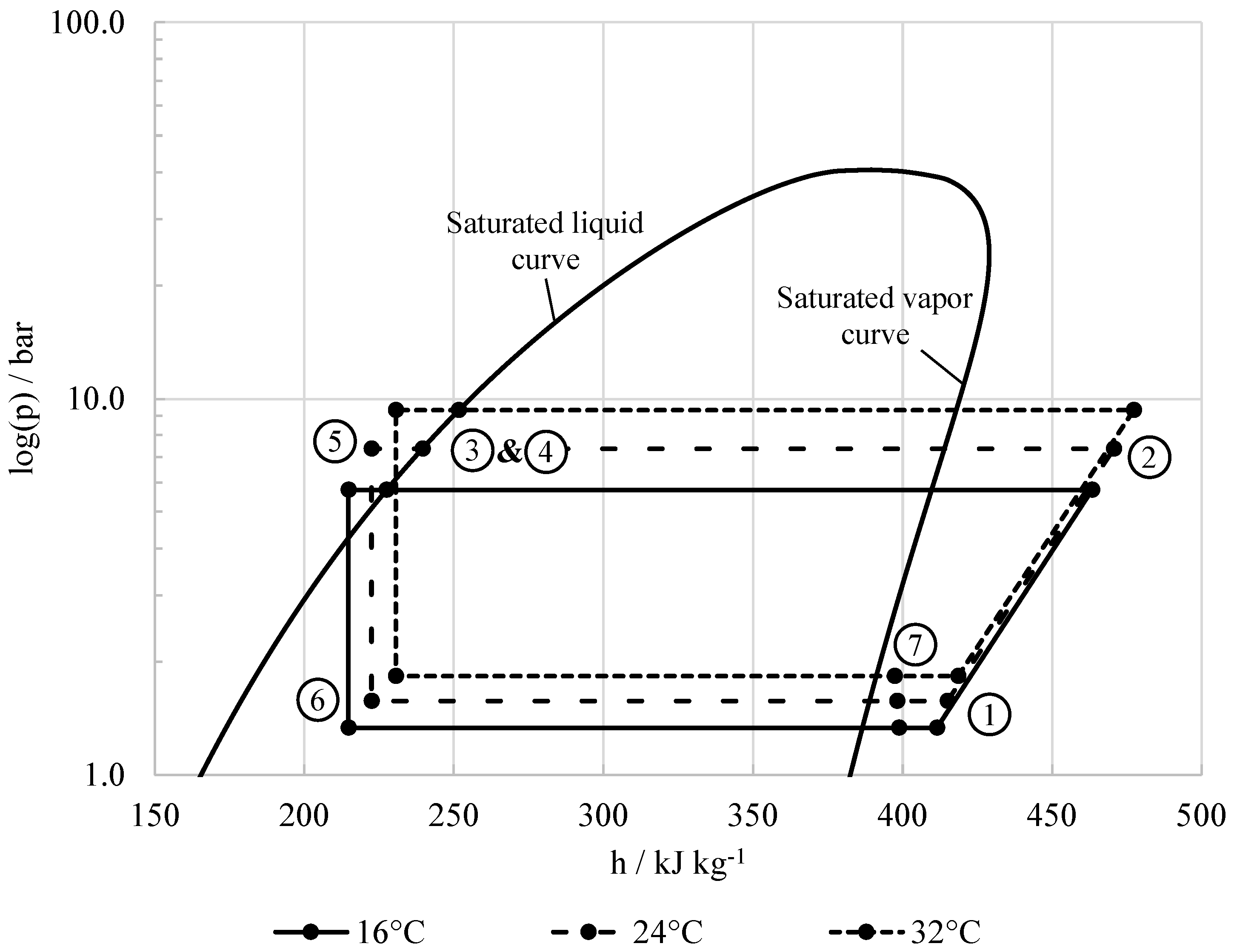
The resulting thermodynamic states are shown in the pressure–enthalpy diagram in Figure 9. Increasing condenser inlet temperature leads to higher condensing pressures, which in turn affect the evaporation temperature and result in variations of both the refrigerant superheat and the evaporator cooling load. This behavior is quantified in

Table 3. Quantitative comparison of direct and inverse problem results for varying condenser antifrogen inlet temperatures.

	Direct Problem (Simulation)				Inverse Problem (Set-Point Tracking)
${\mathit{T}}_{\mathit{i},\mathbf{af},\mathbf{cond}}$/°C	${\dot{\mathit{Q}}}_{\mathbf{evap}}$ /kW	$\mathbf{\Delta }{\mathit{T}}_{\mathbf{sh}}$ /K	$\mathit{\omega }$ /min−1	${\mathit{A}}_{\mathit{v}}$ /–	${\dot{\mathit{Q}}}_{\mathbf{evap}}$ /kW	$\mathbf{\Delta }{\mathit{T}}_{\mathbf{sh}}$ /K	$\mathit{\omega }$ /min−1	${\mathit{A}}_{\mathit{v}}$ /–
16	11.9	18.1	1500	0.4	15.0	5.0	1221	0.534
24	13.1	13.9	1500	0.4	15.0	5.0	1350	0.471
32	14.1	9.86	1500	0.4	15.0	5.0	1508	0.427

, where the compressor rotational speed $\omega$ and the expansion valve opening $A_v$ are held constant, while the resulting cooling load and superheat vary with the condenser operating condition. These effects motivate the inverse problem formulation discussed next.

4.2. Inverse Problem: Set-Point Regulation of Superheat and Cooling Load

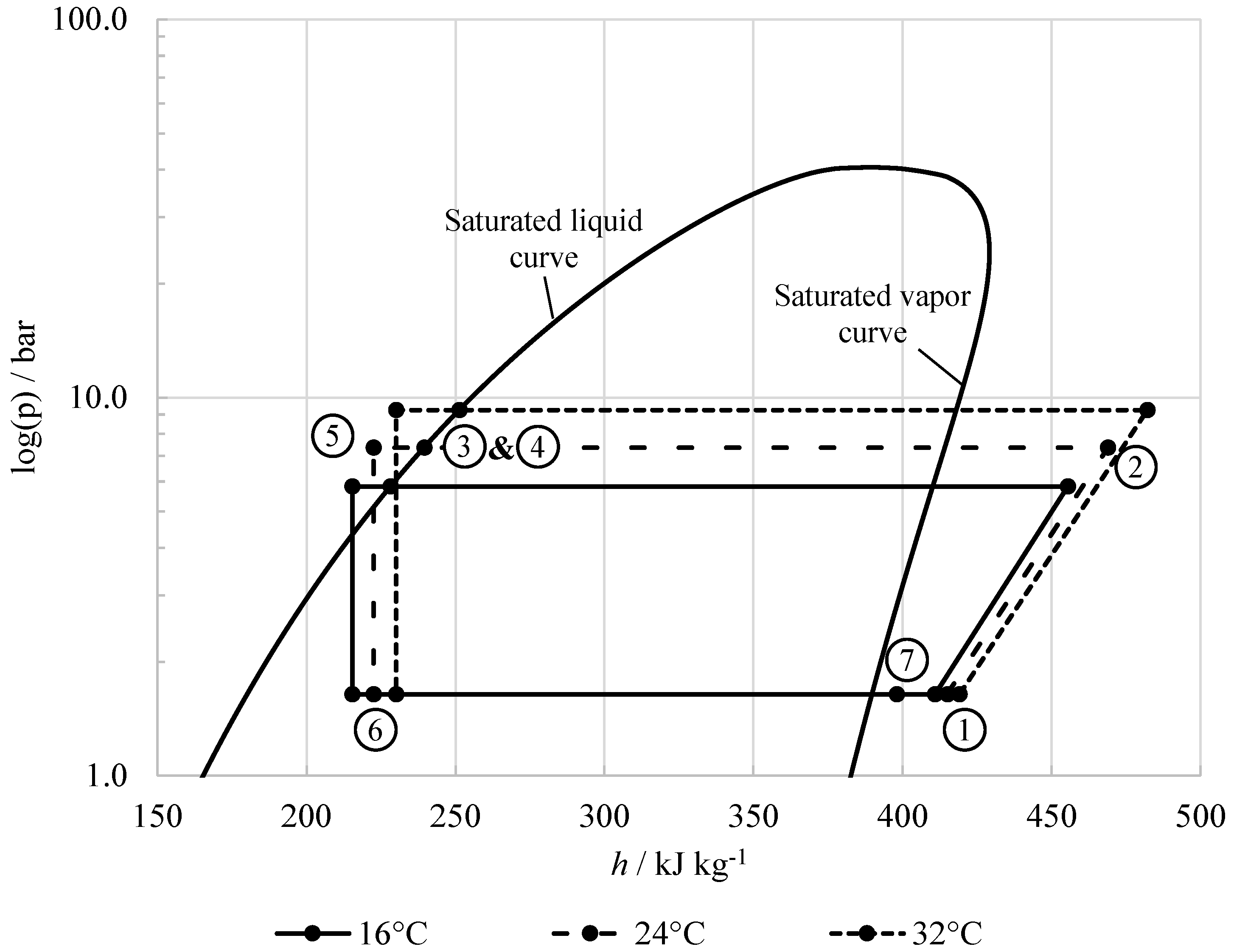
In practical refrigeration systems, the refrigerant superheat at the evaporator outlet, $\Delta T_{\mathrm{sh}}$, and the evaporator cooling load, ${\dot{Q}}_{\mathrm{evap}}$, are typically regulated to prescribed set-point values. In the present work, this operating mode is formulated as an inverse steady-state problem in the SAND setting: selected actuator inputs are treated as decision variables and solved for simultaneously with the tearing variables, while the same tearing-reduced steady-state feasibility equations are enforced. The resulting operating points are visualized in the pressure–enthalpy diagram in Figure 10 and summarized in Table 3.

We treat the compressor speed $\omega$ and the normalized expansion valve opening $A_v$ as variable inputs,

$${\mathbf{u}}^{var}={\left[\begin{array}{cc}\omega & A_v\end{array}\right]}^{\top },$$

(63)

while all antifrogen-side boundary conditions are kept fixed and collected in

$${\mathbf{u}}^{fix}={\left[\begin{array}{cccccc}{p}_{i,\mathrm{af},\mathrm{cond}}& h_{i,\mathrm{af},\mathrm{cond}}& {\dot{m}}_{i,\mathrm{af},\mathrm{cond}}& p_{i,\mathrm{af},\mathrm{evap}}& h_{i,\mathrm{af},\mathrm{evap}}& {\dot{m}}_{i,\mathrm{af},\mathrm{evap}}\end{array}\right]}^{\top }.$$

(64)

The quantities subject to prescribed set-point values are evaluated from the reconstructed steady-state solution as

$$\left[\begin{array}{c}{\dot{Q}}_{\mathrm{evap}}\\ \Delta T_{\mathrm{sh}}\end{array}\right]=g(\mathbf{x};\mathbf{u}),$$

(65)

where $\mathbf{x}=\mathbf{x}(\mathbf{z};\mathbf{u})$ denotes the reconstructed steady-state port-variable vector.

The corresponding set-point errors are defined as

$$e_1={\dot{Q}}_{\mathrm{evap}}^{sp}-{\dot{m}}_{i,\mathrm{r},\mathrm{evap}}·\left(h_{o,\mathrm{r},\mathrm{evap}}-h_{i,\mathrm{r},\mathrm{evap}}\right),$$

(66)

and

$$e_2=\Delta T_{\mathrm{sh}}^{sp}-\left(T_{o,\mathrm{r},\mathrm{evap}}-T_s\left(p_{o,\mathrm{r},\mathrm{evap}}\right)\right),$$

(67)

where the superscript $sp$ denotes the prescribed set-point value and $\mathrm{r}$ denotes the refrigerant side. Accordingly, ${\dot{m}}_{i,\mathrm{r},\mathrm{evap}}$, $h_{i,\mathrm{r},\mathrm{evap}}$, and $h_{o,\mathrm{r},\mathrm{evap}}$ denote the refrigerant-side inlet mass flow rate and the inlet and outlet enthalpies of the evaporator, respectively. The evaporator cooling load is therefore evaluated from the refrigerant-side enthalpy rise across the evaporator. Furthermore, $p_{o,\mathrm{r},\mathrm{evap}}$ and $T_{o,\mathrm{r},\mathrm{evap}}$ denote the refrigerant-side outlet pressure and temperature of the evaporator, respectively, while $T_s\left(p\right)$ denotes the saturation temperature at pressure p. Both errors vanish when the prescribed set-point values are matched exactly.

Given the tearing-reduced residual Equation (59) together with the additional closure constraint (62), the inverse problem is posed as

$$\begin{array}{cc}\hfill \underset{\mathbf{z},{\mathbf{u}}^{var}}{min}& w_1{e}_1^2+w_2{e}_2^2\hfill \\ \hfill \mathrm{subject}\mathrm{to}& p_{i,\mathrm{co}}-p_{o,\mathrm{ihx},\mathrm{c}}(\mathbf{z},{\mathbf{u}}^{var})=0,\hfill \\ \hfill & h_{i,\mathrm{co}}-h_{o,\mathrm{ihx},\mathrm{c}}(\mathbf{z},{\mathbf{u}}^{var})=0,\hfill \\ \hfill & p_{i,\exp }-p_{o,\mathrm{ihx},\mathrm{h}}(\mathbf{z},{\mathbf{u}}^{var})=0,\hfill \\ \hfill & h_{i,\exp }-h_{o,\mathrm{ihx},\mathrm{h}}(\mathbf{z},{\mathbf{u}}^{var})=0,\hfill \\ \hfill & {\dot{m}}_{i,\exp }\left(\mathbf{z}\right)-{\dot{m}}_{o,\mathrm{ihx},\mathrm{h}}(\mathbf{z},{\mathbf{u}}^{var})=0,\hfill \\ \hfill & h_{o,\mathrm{r},\mathrm{cond}}(\mathbf{z},{\mathbf{u}}^{var})-h_s\left(p_{o,\mathrm{r},\mathrm{cond}}(\mathbf{z},{\mathbf{u}}^{var})\right)=0,\hfill \\ \hfill & 750\le \omega \le 3500,\hfill \\ \hfill & 0\le A_v\le 1,\hfill \end{array}$$

(68)

A weighted least-squares objective is used to penalize deviations from the prescribed cooling-load and superheat set-points. The weights $w_i$ are chosen such that both tracking objectives contribute comparably despite their different physical units. The resulting problem (68) is solved using a nonlinear programming solver (SLSQP in the present implementation [37]). As shown in Table 3, the prescribed set-points are satisfied for all considered condenser inlet temperatures by adjusting $\omega$ and $A_v$ accordingly. In contrast to the direct problem, where $\omega$ and $A_v$ are fixed and the operating point changes with $T_{i,\mathrm{af},\mathrm{cond}}$, the inverse formulation enforces the same set-point values $({\dot{Q}}_{\mathrm{evap}}^{sp},\Delta T_{\mathrm{sh}}^{sp})$ across all considered condenser inlet temperatures by adapting $\omega$ and $A_v$.

5. Discussion

This section discusses the obtained results in the context of existing steady-state modeling and optimization approaches for thermal–hydraulic networks. The discussion is structured around (i) the numerical implications of the SAND formulation, (ii) the role of tearing in reducing the nonlinear solution effort, and (iii) practical considerations and limitations for real-world applications.

5.1. Interpretation of Direct and Inverse Problem Results

The direct simulations show that varying $T_{i,\mathrm{af},\mathrm{cond}}$ changes the condensing pressure level and thereby shifts the operating point of the cycle, leading to substantial variations in both ${\dot{Q}}_{\mathrm{evap}}$ and $\Delta T_{\mathrm{sh}}$ when $\omega$ and $A_v$ are held constant (Table 3). This behavior is consistent with the strong coupling between condenser boundary conditions and the evaporator outlet state in vapor-compression systems. In contrast, the inverse formulation enforces the prescribed set-points across all operating points by adjusting $\omega$ and $A_v$. This illustrates how set-point tracking can be handled within the same steady-state network model once selected inputs are treated as decision variables rather than prescribed quantities.

5.2. Implications of SAND Compared with Nested Forward-Simulation Approaches

A key practical consequence of the proposed formulation is that inverse problems are solved without an outer loop that repeatedly calls a direct steady-state solver. Instead, steady-state feasibility and set-point tracking are handled simultaneously within a single constrained optimization problem. This is particularly relevant in cases where the direct problem itself is computationally expensive or numerically difficult to solve. At the same time, SAND formulations introduce a larger set of simultaneous decision variables and constraints, which may increase sensitivity to scaling, variable bounds, and initial guesses. Appropriate problem formulation and numerical scaling therefore remain important for reliable convergence.

5.3. Role of Tearing and Reduced Nonlinear Iteration

The tripartite-graph-based tearing strategy restricts nonlinear iterations to a reduced set of tearing variables, while the remaining variables are reconstructed by forward evaluation of the executable component sequence. This separation can be advantageous in network-scale problems, where fully implicit acausal formulations may lead to large coupled algebraic systems.

In the presented test case, the tearing variables and the corresponding residual equations define a compact nonlinear core that is used consistently for both root finding in the direct problem and constrained optimization in the inverse problem, while the modularity of the component-based network formulation is preserved. Although this example illustrates the role of tearing in reducing the nonlinear system to be solved, its computational benefit for larger networks cannot be quantified from the present test case alone. In general, the computational effort depends on the network topology, the number of tearing variables retained after structural reduction, the complexity of the selected component models, the cost of thermodynamic property evaluations, any component-internal nonlinear solution procedures, and the numerical solver employed. The proposed methodology should therefore be understood as a structural reduction framework whose computational advantage is expected to be most pronounced when only a comparatively small nonlinear core remains after tearing.

5.4. Practical Limitations and Robustness Considerations

Although the prescribed set-point targets are achieved throughout the demonstrated operating range, existence and uniqueness of inverse solutions are not guaranteed in general. In practice, feasibility may be lost due to actuator saturation or thermodynamic restrictions. This is precisely why inverse problems are formulated here as residual-constrained optimization problems. Such a formulation can systematically accommodate operational bounds, additional constraints, and possible infeasibilities. Moreover, the present component models are steady-state models and therefore do not capture transient control dynamics. Accordingly, the proposed inverse formulation should be interpreted as a steady-state set-point determination problem, i.e., as the computation of a static operating point. In this form, it can provide a useful basis for supervisory control, design studies, or the initialization of dynamic simulations.

In addition to these modeling and application-related limitations, the computational performance of the proposed methodology for larger thermal–hydraulic networks remains to be systematically assessed. Benchmark comparisons with established simulation and optimization tools would be required to quantify the computational cost and scaling behavior of the tearing-reduced formulation under comparable component models, thermodynamic-property formulations, solver tolerances, and implementation settings. Such benchmark studies are therefore considered an important direction for future work.

6. Conclusions

This paper presented a unified methodology for the modeling and solution of direct and inverse optimization problems in steady-state thermal–hydraulic networks. The proposed methodology combines causal (input–output) component representations with acausal (implicit) balance relations at the network level and uses a tripartite-graph-based tearing strategy to reduce the assembled algebraic system to a compact tearing-reduced formulation.

For direct problems with prescribed system inputs, the steady-state solution is obtained by solving the tearing-reduced residual equations with a nonlinear root-finding method. For inverse problems, the same steady-state network model is embedded in a simultaneous analysis and design (SAND) formulation, in which the tearing variables and selected system inputs are treated as unknowns simultaneously, while the governing balance equations and operational constraints are enforced directly. In this way, inverse problems such as set-point tracking can be formulated within the same mathematical structure as the direct problem, without introducing an outer loop based on repeated forward simulations.

The methodology was demonstrated on a steady-state vapor-compression refrigeration cycle with compressor speed and expansion valve opening as actuation variables. For the direct problem, the model predicts the change in operating point caused by varying condenser inlet conditions. For the inverse problem, the same tearing-reduced network formulation was used to determine actuator settings that satisfy prescribed cooling-load and superheat targets under different operating conditions. This illustrates how direct simulation and set-point-driven inverse operation can be handled consistently within a single modeling workflow.

Implemented as an open-source Python module, the proposed approach provides a transparent and reproducible basis for steady-state simulation and inverse problem solving in coupled thermal–hydraulic networks. Beyond the demonstrated set-point tracking problem, the formulation also provides a foundation for more general constrained optimization tasks in system design and operation.

References

1. International Energy Agency. Energy Efficiency 2024; Technical Report; International Energy Agency: Paris, France, 2024. [Google Scholar]
2. Gumpert, B.; Wieland, C.; Spliethoff, H. Thermo-hydraulic simulation of district heating systems. Geothermics 2019, 82, 244–253. [Google Scholar] [CrossRef]
3. Wang, D.; Li, X.; Marquant, J.; Carmeliet, J.; Orehounig, K. Advancing the Thermal Network Representation for the Optimal Design of Distributed Multi-Energy Systems. Front. Energy Res. 2021, 9, 668124. [Google Scholar] [CrossRef]
4. Fiorentini, M.; Heer, P.; Baldini, L. Design optimization of a district heating and cooling system with a borehole seasonal thermal energy storage. Energy 2023, 262, 125464. [Google Scholar] [CrossRef]
5. Witte, F.; Tuschy, I. TESPy: Thermal Engineering Systems in Python. J. Open Source Softw. 2020, 5, 2178. [Google Scholar] [CrossRef]
6. Franke, R.; Casella, F.; Otter, M.; Proelss, K.; Sielemann, M.; Wetter, M. Standardization of Thermo-Fluid Modeling in Modelica.Fluid. In Proceedings of the 7th International Modelica Conference, Como, Italy, 20–22 September 2009; pp. 122–131. [Google Scholar]
7. Lee, A.; Ghouse, J.H.; Eslick, J.C.; Laird, C.D.; Siirola, J.D.; Zamarripa, M.A.; Gunter, D.; Shinn, J.H.; Dowling, A.W.; Bhattacharyya, D.; et al. The IDAES Process Modeling Framework and Model Library—Flexibility for Process Simulation and Optimization. J. Adv. Manuf. Process. 2021, 3, e10095. [Google Scholar] [CrossRef]
8. Ortega, J.M.; Rheinboldt, W.C. Iterative Solution of Nonlinear Equations in Several Variables; Academic Press: Cambridge, MA, USA, 1970. [Google Scholar]
9. Kelley, C.T. Solving Nonlinear Equations with Newton’s Method; SIAM: Philadelphia, PA, USA, 2003. [Google Scholar]
10. Zimmer, D. Robust Object-Oriented Formulation of Directed Thermofluid Stream Networks. Math. Comput. Model. Dyn. Syst. 2020, 26, 204–233. [Google Scholar] [CrossRef]
11. Steward, D.V. Partitioning and Tearing Systems of Equation. J. Soc. Ind. Appl. Math. Ser. B Numer. Anal. 1965, 2, 345–365. [Google Scholar] [CrossRef]
12. Dulmage, A.L.; Mendelsohn, N.S. Coverings of Bipartite Graphs. Can. J. Math. 1958, 10, 517–534. [Google Scholar] [CrossRef]
13. Elmqvist, H.; Otter, M. Methods for Tearing Systems of Equations in Object-Oriented Modeling. In Proceedings of the European Simulation Multiconference, Barcelona, Spain, 1–3 June 1994; pp. 326–332. [Google Scholar]
14. Huang, R.; Aute, V.; Ling, J. A tripartite graph based methodology for steady-state solution of generalized multi-mode vapor compression systems. Appl. Therm. Eng. 2021, 185, 116385. [Google Scholar] [CrossRef]
15. Bell, I.H.; Wronski, J.; Quoilin, S.; Lemort, V. Pure and Pseudo-Pure Fluid Thermophysical Property Evaluation and the Open-Source Thermophysical Property Library CoolProp. Ind. Eng. Chem. Res. 2014, 53, 2498–2508. [Google Scholar] [CrossRef] [PubMed]
16. Ghiaus, C. Causality issue in the heat balance method for calculating the design heating and cooling load. Energy 2013, 50, 292–301. [Google Scholar] [CrossRef]
17. Ghiaus, C. Computational psychrometric analysis as a control problem: Case of cooling and dehumidification systems. Int. J. Build. Perform. Simul. 2022, 15, 21–38. [Google Scholar] [CrossRef]
18. Wang, J.; Zhou, Z.; Zhao, J. A Method for the Steady-State Thermal Simulation of District Heating Systems and Model Parameters Calibration. Energy Convers. Manag. 2016, 120, 294–305. [Google Scholar] [CrossRef]
19. Maldonado, D.; Schönfeldt, P.; Torio, H.; Witte, F.; Füting, M. Validation of a calibrated steady-state heat network model using measured data. Appl. Therm. Eng. 2024, 248, 123267. [Google Scholar] [CrossRef]
20. Zhou, R.; Zhang, T.; Catano, J.; Wen, J.T.; Michna, G.J.; Peles, Y.; Jensen, M.K. The steady-state modeling and optimization of a refrigeration system for high heat flux removal. Appl. Therm. Eng. 2010, 30, 2347–2356. [Google Scholar] [CrossRef]
21. Ghasemi, H.; Paci, M.; Tizzanini, A.; Mitsos, A. Modeling and optimization of a binary geothermal power plant. Energy 2013, 50, 412–428. [Google Scholar] [CrossRef]
22. Hendricks, E.S.; Gray, J.S. pyCycle: A tool for efficient optimization of gas turbine engine cycles. Aerospace 2019, 6, 87. [Google Scholar] [CrossRef]
23. Gray, J.S.; Hwang, J.T.; Martins, J.R.R.A.; Moore, K.T.; Naylor, B.A. OpenMDAO: An Open-Source Framework for Multidisciplinary Design, Analysis, and Optimization. Struct. Multidiscip. Optim. 2019, 59, 1075–1104. [Google Scholar] [CrossRef]
24. Balling, R.J.; Sobieszczanski-Sobieski, J. Optimization of Coupled Systems: A Critical Overview of Approaches. AIAA J. 1996, 34, 6–17. [Google Scholar] [CrossRef]
25. Martins, J.R.R.A.; Ning, A. Engineering Design Optimization; Cambridge University Press: Cambridge, UK, 2022. [Google Scholar] [CrossRef]
26. Biegler, L.T.; Ghattas, O.; Heinkenschloss, M.; van Bloemen Waanders, B. (Eds.) Large-Scale PDE-Constrained Optimization; Lecture Notes in Computational Science and Engineering; Springer: Berlin/Heidelberg, Germany, 2003; Volume 30. [Google Scholar] [CrossRef]
27. Günther, S.; Gauger, N.R.; Wang, Q. Simultaneous Single-Step One-Shot Optimization with Unsteady PDEs. J. Comput. Appl. Math. 2016, 294, 12–22. [Google Scholar] [CrossRef]
28. Ghiaus, C.; Allard, F. Potential for free-cooling by ventilation. Sol. Energy 2006, 80, 402–413. [Google Scholar] [CrossRef]
29. Inard, C.; Pfafferott, J.; Ghiaus, C. Free-running temperature and potential for free cooling by ventilation: A case study. Energy Build. 2011, 43, 2705–2711. [Google Scholar] [CrossRef]
30. TESPy Development Team. TESPy Documentation: Networks. 2026. Available online: https://tespy.readthedocs.io/en/dev/building_blocks/networks.html (accessed on 17 April 2026).
31. TESPy Development Team. TESPy Documentation: Components. 2026. Available online: https://tespy.readthedocs.io/en/dev/building_blocks/components.html (accessed on 17 April 2026).
32. TESPy Development Team. TESPy Documentation: Thermal Power Plant Efficiency Optimization. 2026. Available online: https://tespy.readthedocs.io/en/v0.9/tutorials/pygmo_optimization.html (accessed on 17 April 2026).
33. Bitzer Software, 6.17.9; BITZER SOFTWARE: Sindelfingen, Germany, 2013. Available online: https://www.bitzer.de (accessed on 23 December 2025).
34. Ma, J.; Kim, D.; Braun, J.E.; Horton, W.T. Development and validation of a dynamic modeling framework for air-source heat pumps under cycling of frosting and reverse-cycle defrosting. Energy 2023, 272, 127030. [Google Scholar] [CrossRef]
35. Osborne, M.R. On shooting methods for boundary value problems. J. Math. Anal. Appl. 1969, 27, 417–433. [Google Scholar] [CrossRef]
36. von Böckh, P.; Wetzel, T. Wärmeübertragung, 5th ed.; Springer: Berlin/Heidelberg, Germany, 2014. [Google Scholar]
37. Kraft, D. A Software Package for Sequential Quadratic Programming; Forschungsbericht- Deutsche Forschungs- und Versuchsanstalt fur Luft- und Raumfahrt: Köln, Germany, 1988. [Google Scholar]
Figure 1. Hybrid modeling view: components are evaluated through causal interfaces at the component level, while system-level interconnections are enforced through acausal junction balance equations.
Energies 19 02587 g001
Figure 2. Component modeling views: (a) externally causal evaluation map f c ; (b) the same interface with an encapsulated internally implicit solve for component-internal states.
Energies 19 02587 g002
Figure 3. Schematic component and corresponding causal model representation of a pressure-based compressor and a mass-flow-based heat exchanger.
Energies 19 02587 g003
Figure 4. Illustrative coupling through a junction: compressor outlet connected to a heat-exchanger inlet. Junction balance equations enforce mass and energy conservation and pressure continuity across connected ports.
Energies 19 02587 g004
Figure 5. Basic junction connection patterns used in the network assembly (merge (a) and split (b) configurations).
Energies 19 02587 g005
Figure 6. Illustrative network topologies showing (a) an open fluid loop and (b) a closed fluid loop. Closed loops typically require additional independent closure relations to ensure structural well-posedness.
Energies 19 02587 g006
Figure 7. Schematic model of the vapor-compression refrigeration cycle used in the test case. The numbered labels identify the thermodynamic state points at the component inlets and outlets and are used throughout the analysis to refer to the corresponding refrigerant states.
Energies 19 02587 g007
Figure 8. Discretization approach used in the evaporator and condenser model.
Energies 19 02587 g008
Figure 9. Simulated thermodynamic states for condenser antifrogen inlet temperatures of 16 °C, 24 °C, and 32 °C, obtained from the direct problem. The numbered labels identify the thermodynamic state points of the refrigerant cycle according to the schematic representation in Figure 7.
Energies 19 02587 g009
Figure 10. Simulated thermodynamic states for condenser antifrogen inlet temperatures of 16 °C, 24 °C, and 32 °C, obtained from the inverse problem. The numbered labels identify the thermodynamic state points of the refrigerant cycle according to the schematic representation in Figure 7.
Energies 19 02587 g010