A Benchmark System for Verifying the Harmonic Amplification Mechanism of Wideband Oscillations

Abstract

To verify the harmonic amplification mechanism of wideband oscillations, this paper constructs a benchmark system. Firstly, the theoretical framework of the harmonic amplification mechanism for wideband oscillations is elaborated. Subsequently, the structure and parameters of the benchmark system are presented. Based on the s-domain nodal admittance matrix method, the resonant characteristics of the benchmark system, including resonance frequency, damping ratio, and nodal voltage mode shape, are calculated. Using electromagnetic transient simulation, the time-domain waveforms of the current, voltage, and power of the benchmark system under typical operating conditions are obtained, and harmonic decomposition of these waveforms is performed. By comparing and analyzing the harmonic components of current, voltage, and active power with the resonant characteristic quantities, the harmonic amplification mechanism of wideband oscillations is verified. The applicability of analyzing the harmonic amplification effect based on the positive-sequence network model is demonstrated. It is shown that the resonance frequency, damping ratio, nodal voltage mode shape, and resonant peak voltage are four key factors determining the harmonic amplification effect. Finally, the relationship between the frequency of the oscillatory power component and the frequency of the harmonic source is revealed.

1. Introduction

Driven by the energy transition and the “carbon peak and carbon neutrality” goals, the power system is accelerating its evolution towards a “double-high” form characterized by a high proportion of renewable energy and a high proportion of power electronic devices. This has made the previously rare issue of wideband oscillations increasingly common, posing a key threat to the safe and stable operation of the power grid [1,2,3,4].

However, the understanding of the mechanism behind wideband oscillations remains quite inadequate. The prevailing explanation in the industry is the “negative resistance” mechanism [5,6,7,8,9], which suggests that wideband oscillations are caused by the “negative resistance” effect of power electronic devices. Since the theoretical foundation of the “negative resistance” mechanism lies in the incremental impedance model of power electronic devices, applying this model to analyze wideband oscillations in AC power grids encounters a dilemma, namely the “cutting the feet to fit the shoes” predicament and the “walking into a dead-end path” predicament [10,11]. Consequently, the analysis and control of wideband oscillations in AC power grids based on the “negative resistance” mechanism are theoretically invalid. In fact, despite the existence of a substantial body of literature on analyzing wideband oscillations in AC power grids based on the “negative resistance” mechanism, it is difficult to find a paper that provides test systems to prove the correctness of this mechanism. This is also a significant factor that undermines the credibility of the “negative resistance” mechanism.

The author’s previous work [11] proposed a “harmonic amplification” mechanism for wideband oscillations, rejecting the traditional “negative resistance” theory and providing a novel perspective for the analysis of wideband oscillations in new energy power systems. This paper will construct a benchmark system based on a real physical system to validate the “harmonic amplification” mechanism for wideband oscillations proposed in Reference [11]. The subsequent sections of this paper will describe the theoretical foundation of the “harmonic amplification” mechanism for wideband oscillations, present the benchmark system designed to verify this mechanism, demonstrate the wideband oscillation characteristics of the benchmark system under a specific operating condition, reveal the four decisive factors of “harmonic amplification” in the power grid, and derive the intrinsic relationship between the frequency of oscillatory power components and the frequency of harmonic sources. Additionally, the “harmonic amplification” analysis method based on the s-domain nodal admittance matrix approach will be validated.

2. Theoretical Foundation of the Harmonic Amplification Mechanism for Wideband Oscillations

Reference [11] proposes the “harmonic amplification” mechanism for wideband oscillations. Its theoretical framework consists of the following five components.

2.1. Two Kinds of Wideband Converter Models

Power electronic devices can be described using either a wideband voltage source converter model or a wideband current source converter model [11]. For common two-level and three-level voltage source converters, due to the effects of background harmonics and dead-time effects, the output voltage and current waveforms are not strictly periodic but rather periodic but not completely repeating waveforms [12,13,14,15,16,17]. For submodule cascaded converters, the capacitor voltage balancing control of submodules is often implemented using some sorting algorithm [10], which results in the synthesized internal electromotive force not being a strictly periodic waveform either, but rather a periodic but not completely repeating waveform. Theoretically, the aforementioned periodic but not completely repeating waveforms can be understood as strictly periodic waveforms superimposed with white noise. The harmonic orders of a strictly periodic waveform are positive integers, but the harmonic orders of white noise are continuous variables. Therefore, for the aforementioned periodic but not completely repeating waveforms, the harmonic orders they contain are not necessarily positive integers. Hence, the harmonic orders in the wideband model of power electronic devices can be understood as continuous variables greater than 1.

2.2. The Applicability of the Positive Sequence Grid Model for Harmonic Amplification Analysis

The positive-sequence grid model is uniformly applicable for “harmonic amplification” analysis [11]. The decision to use only the positive-sequence network model when analyzing “harmonic amplification” problems is determined by the following two factors. On one hand, power electronic devices acting as harmonic sources generally do not inject zero-sequence components into the power network. For instance, line commutated converters used in HVDC transmission prevent zero-sequence current from flowing into the grid through transformer connections [18]. Consequently, according to the principle of the symmetrical component method, only positive-sequence and negative-sequence components of harmonics flow into the power grid. On the other hand, the positive-sequence and negative-sequence circuit models for static elements such as transmission lines and transformers in the power system are identical [19]. Therefore, the positive-sequence network model can be uniformly applied to analyze both positive-sequence and negative-sequence harmonic components from power electronic devices.

2.3. Consistency Between Network Resonance Modes and Eigenvalues of the System State Equations

Power grids generally possess weakly damped resonance modes. In their classic work “Electric Network Theory” published in 1969, N. Balabanian et al. presented a fundamental theorem of electric networks [20]: For a linear time-invariant network, the determinant of its s-domain loop impedance matrix, the determinant of its s-domain nodal admittance matrix, and the characteristic polynomial of the system’s state equations share identical non-zero zeros. This theorem essentially provides the definition of resonance modes in electric networks, i.e., the resonance modes of an electric network are precisely the eigenvalues of the system’s state equations. This unifies the definition of electric network resonance modes within the framework of the state-space model of modern control theory [21]. For each resonance mode, its real part characterizes the damping magnitude, and its imaginary part characterizes the resonance frequency. Given that resistance components in actual power grids are very small, most resonance modes in power grids are weakly damped modes.

2.4. Inverse Relationship Between Resonant Peak Voltage and Modal Damping Ratio

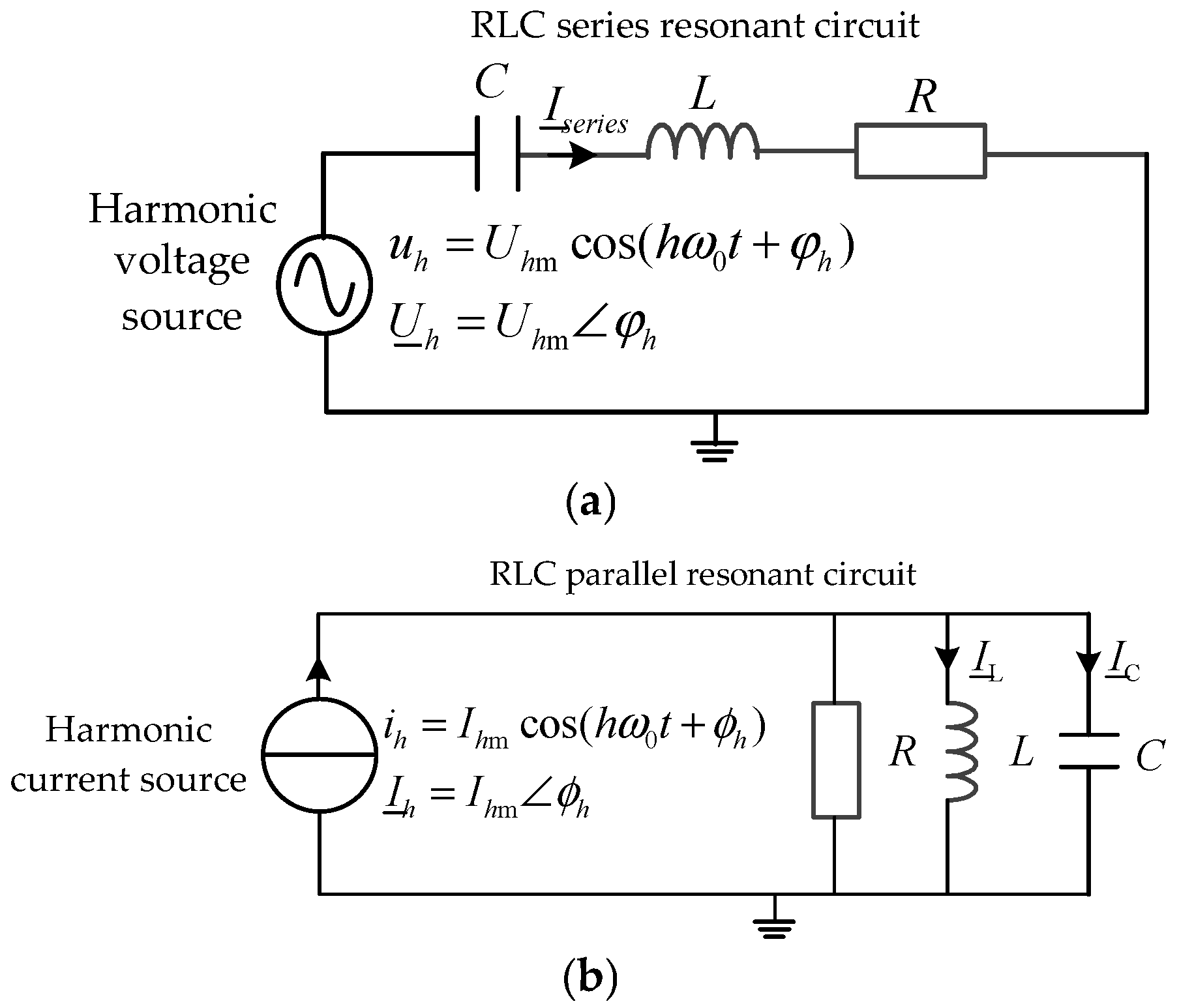
The resonant peak voltage is inversely proportional to the damping ratio of the resonance mode. This can be illustrated using the most fundamental RLC series resonant circuit and RLC parallel resonant circuit. For the RLC series resonant circuit and RLC parallel resonant circuit shown in Figure 1, R, L, and C represent resistance, inductance, and capacitance respectively; h is the harmonic order; ω₀ is the fundamental angular frequency; φ_h is the initial phase angle of the harmonic voltage source; ϕ_h is the initial phase angle of the harmonic current source; U_hm is the amplitude of the harmonic voltage source; I_hm is the amplitude of the harmonic current source; u_h and U_h are the instantaneous value and phasor of the harmonic voltage source, respectively; i_h and I_h are the instantaneous value and phasor of the harmonic current source, respectively; I_series is the phasor of the harmonic current flowing through the series resonant circuit; I_L and I_C are the phasors of the harmonic currents flowing through L and C in the parallel resonant circuit.

First, examine the RLC series resonant circuit in Figure 1. The characteristic equation of this circuit is [11]:

$$s^2+{\displaystyle \frac{R}{L}}s+{\displaystyle \frac{1}{LC}}=0$$

(1)

Comparing with the standard form of the characteristic equation for a second-order system $s^2+2\zeta s+{\omega }_n^2=0$, the undamped resonant angular frequency ω_n and damping ratio ζ are obtained as:

$$\left\{\begin{array}{c}{\omega }_n={\displaystyle \frac{1}{\sqrt{LC}}}\\ \zeta ={\displaystyle \frac{1}{2}}{\displaystyle \frac{R}{{\omega }_{n}L}}={\displaystyle \frac{1}{2Q}}\end{array}\right.$$

(2)

In Equation (2), Q = ω_nL/R, which is referred to as the quality factor of the series resonant circuit. On the other hand, ω_n is also the series resonant angular frequency of the RLC series resonant circuit. Under the condition of series resonance, the voltage across the capacitor C and the inductor L are equal in magnitude but opposite in direction, thus canceling each other out. Next, the expression for the voltage magnitude across the inductor L is derived.

$$U_{\mathrm{L}}=\left|(\mathrm{j}{\omega }_{n}L){\underset{\_}{I}}_{series}\right|=\left|(\mathrm{j}{\omega }_{n}L){\displaystyle \frac{U_{hm}\angle {\phi }_h}{R}}\right|=U_{hm}{\displaystyle \frac{{\omega }_{n}L}{R}}=U_{hm}Q=U_{hm}{\displaystyle \frac{1}{2\zeta }}$$

(3)

We refer to U_L in Equation (3) as the resonant peak voltage. It is evident that U_L is inversely proportional to the damping ratio ζ, and when the system is undamped (ζ = 0), U_L = ∞.

Next, examine the RLC parallel resonant circuit in Figure 1. The characteristic equation of this circuit is [11]:

$$s^2+{\displaystyle \frac{1}{RC}}s+{\displaystyle \frac{1}{LC}}=0$$

(4)

Comparing with the standard form of the characteristic equation for a second-order system ($s^2+2\zeta s+{\omega }_n^2=0$), the undamped resonant angular frequency ω_n and damping ratio ζ are obtained as:

$$\left\{\begin{array}{c}{\omega }_n={\displaystyle \frac{1}{\sqrt{LC}}}\\ \zeta ={\displaystyle \frac{1}{2{\omega }_{n}RC}}={\displaystyle \frac{1}{2}}{\displaystyle \frac{{\omega }_{n}L}{R}}={\displaystyle \frac{1}{2q}}\end{array}\right.$$

(5)

In Equation (5), q = R/(ω_nL) is referred to as the quality factor of the parallel resonant circuit. Meanwhile, ω_n is also the parallel resonant angular frequency of the RLC parallel resonant circuit. Under parallel resonance conditions, the currents flowing in the capacitor C and the inductor L are equal in magnitude but opposite in phase, thus canceling each other out. Consequently, under parallel resonance, the current source I_h flows entirely through the resistor R. Obviously, the expression for the voltage magnitude across the inductor L under parallel resonance conditions is:

$$U_{\mathrm{L}}=\left|R{I}_{hm}\angle {\varphi }_h\right|=I_{hm}R=I_{hm}{\omega }_{n}Lq=I_{hm}{\displaystyle \frac{{\omega }_{n}L}{2\zeta }}$$

(6)

We refer to U_L in Equation (6) as the resonant peak voltage. It is evident that U_L is inversely proportional to the damping ratio ζ, and when the system is undamped (ζ = 0), U_L = ∞.

2.5. Physical Meaning of Node Voltage Mode Shapes and Resonant Peak Voltages

The voltage magnitudes at each node in the grid at the resonance frequency can be described by the node voltage mode shape and the resonant peak voltage. Under undamped system conditions, the system eigenvalues are purely imaginary. Let the i-th resonant mode be s_i = jω_i = j2πf_i, where ω_i and f_i are the resonant angular frequency and resonance frequency of the i-th resonant mode, respectively. Therefore, the s-domain node admittance matrix corresponding to the resonant mode s_i is

$${\mathit{Y}}_{\mathrm{node}}(s_i)={\mathit{Y}}_{\mathrm{node}}(\mathrm{j}{\omega }_i)={\mathit{G}}_{\mathrm{node}}(\mathrm{j}{\omega }_i)+\mathrm{j}{B}_{\mathrm{node}}(\mathrm{j}{\omega }_i)=\mathrm{j}{B}_{\mathrm{node}}(\mathrm{j}{\omega }_i)$$

(7)

Because the system is undamped, G_node(jω_i) = 0 in Equation (7), so Y_node(s_i) = jB_node(jω_i), and B_node(jω_i) is a real symmetric matrix. Since s_i is the resonant mode of the system, according to the properties of the s-domain node admittance matrix, it must satisfy [20]:

$$\det ({\mathit{Y}}_{\mathrm{node}}(s_i))=0\Rightarrow \det (\mathrm{j}{\mathit{B}}_{\mathrm{node}}(\mathrm{j}{\omega }_i))=0\Rightarrow \det ({\mathit{B}}_{\mathrm{node}}(\mathrm{j}{\omega }_i))=0$$

(8)

Since det(B_node(jω_i)) = 0, according to matrix theory, the determinant of a matrix equals the product of all its eigenvalues. Therefore, B_node(jω_i) must have a zero eigenvalue λ₁(jω_i) = 0. Let B_node(jω_i) be an n × n matrix. Since B_node(jω_i) is a real symmetric matrix, all its eigenvalues and eigenvectors are real. Let its eigenvalues be λ₁(jω_i), λ₂(jω_i), …, λ_n(jω_i), respectively, and the corresponding right eigenvectors be M₁(jω_i), M₂(jω_i), …, M_n(jω_i). Moreover, M_k(jω_i) (k = 1,2, …,n) are normalized to satisfy the uniqueness condition, i.e., the maximum absolute value of the elements in the column vector M_k(jω_i) (k = 1,2, …,n) is equal to 1. Then, according to matrix theory:

$${\mathit{B}}_{\mathrm{node}}(\mathrm{j}{\omega }_i)=\mathit{M}(\mathrm{j}{\omega }_i)\mathit{\Lambda }(\mathrm{j}{\omega }_i)\mathit{M}{(\mathrm{j}{\omega }_i)}^{-1}$$

(9)

In Equation (9), Λ(jω_i) = diag[λ₁(jω_i), λ₂(jω_i), …, λ_n(jω_i)] is a diagonal matrix with the eigenvalues as its diagonal elements, where λ₁(jω_i) = 0; M(jω_i) = [M₁(jω_i), M₂(jω_i), …, M_n(jω_i)] is the right eigenvector matrix of B_node(jω_i). According to the definition of the s-domain node admittance matrix, we have

$${\mathit{Y}}_{\mathrm{node}}(\mathrm{j}{\omega }_i){\mathit{V}}_{\mathrm{node}}(\mathrm{j}{\omega }_i)={\mathit{I}}_{\mathrm{node}}(\mathrm{j}{\omega }_i)\Rightarrow \mathrm{j}\mathit{B}(\mathrm{j}{\omega }_i){\mathit{V}}_{\mathrm{node}}(\mathrm{j}{\omega }_i)={\mathit{I}}_{\mathrm{node}}(\mathrm{j}{\omega }_i)$$

(10)

In Equation (10), V_node(jω_i) is the node voltage vector of the grid, and I_node(jω_i) is the node injected current vector. Let

$$\left\{\begin{array}{c}{\mathit{U}}_{\mathrm{mode}}(\mathrm{j}{\omega }_i)=\mathit{M}{(\mathrm{j}{\omega }_i)}^{-1}{\mathit{V}}_{\mathrm{node}}(\mathrm{j}{\omega }_i)\\ {\mathit{J}}_{\mathrm{mode}}(\mathrm{j}{\omega }_i)=\mathit{M}{(\mathrm{j}{\omega }_i)}^{-1}{\mathit{I}}_{\mathrm{node}}(\mathrm{j}{\omega }_i)\end{array}\right.$$

(11)

In Equation (11), U_mode(jω_i) and J_mode(jω_i) are referred to as the modal node voltage vector and the modal node injected current vector, respectively. Then, according to Equations (9) and (11), Equation (10) can be transformed into

$${\mathit{U}}_{\mathrm{mode}}(\mathrm{j}{\omega }_i)=-\mathrm{j}\mathit{\Lambda }{(\mathrm{j}{\omega }_i)}^{-1}{\mathit{J}}_{\mathrm{mode}}(\mathrm{j}{\omega }_i)$$

(12)

Let

$${\mathit{U}}_{\mathrm{mode}}(\mathrm{j}{\omega }_i)=\left[\begin{array}{c}{U}_{\mathrm{mode}1}(\mathrm{j}{\omega }_i)\\ U_{\mathrm{mode}2}(\mathrm{j}{\omega }_i)\\ ⋮\\ U_{\mathrm{mod}\mathrm{e}n}(\mathrm{j}{\omega }_i)\end{array}\right],{\mathit{J}}_{\mathrm{mode}}(\mathrm{j}{\omega }_i)=\left[\begin{array}{c}{J}_{\mathrm{mode}1}(\mathrm{j}{\omega }_i)\\ J_{\mathrm{mode}2}(\mathrm{j}{\omega }_i)\\ ⋮\\ J_{\mathrm{mod}\mathrm{e}n}(\mathrm{j}{\omega }_i)\end{array}\right]$$

(13)

Then, Equation (12) becomes

$$\left[\begin{array}{c}{U}_{\mathrm{mode}1}(\mathrm{j}{\omega }_i)\\ U_{\mathrm{mode}2}(\mathrm{j}{\omega }_i)\\ ⋮\\ U_{\mathrm{mode}n}(\mathrm{j}{\omega }_i)\end{array}\right]=-\mathrm{j}\left[\begin{array}{c}{\lambda }_1{(\mathrm{j}{\omega }_i)}^{-1}{J}_{\mathrm{mode}1}(\mathrm{j}{\omega }_i)\\ {\lambda }_2{(\mathrm{j}{\omega }_i)}^{-1}{J}_{\mathrm{mode}2}(\mathrm{j}{\omega }_i)\\ ⋮\\ {\lambda }_n{(\mathrm{j}{\omega }_i)}^{-1}{J}_{\mathrm{mode}n}(\mathrm{j}{\omega }_i)\end{array}\right]$$

(14)

Since ${\lambda }_1{(\mathrm{j}{\omega }_i)}^{-1}=\infty$, and ${\lambda }_2{(\mathrm{j}{\omega }_i)}^{-1},\dots ,{\lambda }_n{(\mathrm{j}{\omega }_i)}^{-1}$ is a finite value, it follows that |U_mode1(jω_i)|>>|U_mode2(jω_i)|, …,|U_mode1(jω_i)|>>|U_moden(jω_i)|. According to Equation (11), we have

$$\begin{array}{ll}\hfill {\mathit{V}}_{\mathrm{node}}(\mathrm{j}{\omega }_i)& =\mathit{M}(\mathrm{j}{\omega }_i){\mathit{U}}_{\mathrm{mode}}(\mathrm{j}{\omega }_i)=[{\mathit{M}}_1(\mathrm{j}{\omega }_i) {\mathit{M}}_2(\mathrm{j}{\omega }_i) \dots {\mathit{M}}_n(\mathrm{j}{\omega }_i)]\left[\begin{array}{c}{U}_{\mathrm{mode}1}(\mathrm{j}{\omega }_i)\\ U_{\mathrm{mode}2}(\mathrm{j}{\omega }_i)\\ ⋮\\ U_{\mathrm{mod}\mathrm{e}n}(\mathrm{j}{\omega }_i)\end{array}\right]\hfill \\ \hfill & =U_{\mathrm{mode}1}(\mathrm{j}{\omega }_i){\mathit{M}}_1(\mathrm{j}{\omega }_i)+U_{\mathrm{mode}2}(\mathrm{j}{\omega }_i){\mathit{M}}_2(\mathrm{j}{\omega }_i)+\dots +U_{\mathrm{mode}n}(\mathrm{j}{\omega }_i){\mathit{M}}_n(\mathrm{j}{\omega }_i)\hfill \\ \hfill & \approx U_{\mathrm{mode}1}(\mathrm{j}{\omega }_i){\mathit{M}}_1(\mathrm{j}{\omega }_i)\hfill \end{array}$$

(15)

According to Equation (15), V_node(jω_i) ≈ U_mode1(jω_i)M₁(jω_i), which means that the node voltage vector V_node(jω_i) differs from the right eigenvector M₁(jω_i) corresponding to the zero eigenvalue λ₁(jω_i) = 0 only by a scaling factor U_mode1(jω_i). Therefore, we define M₁(jω_i) as the node voltage mode shape corresponding to the resonant mode jω_i and |U_mode1(jω_i)| as the resonant peak voltage corresponding to the resonant mode jω_i.

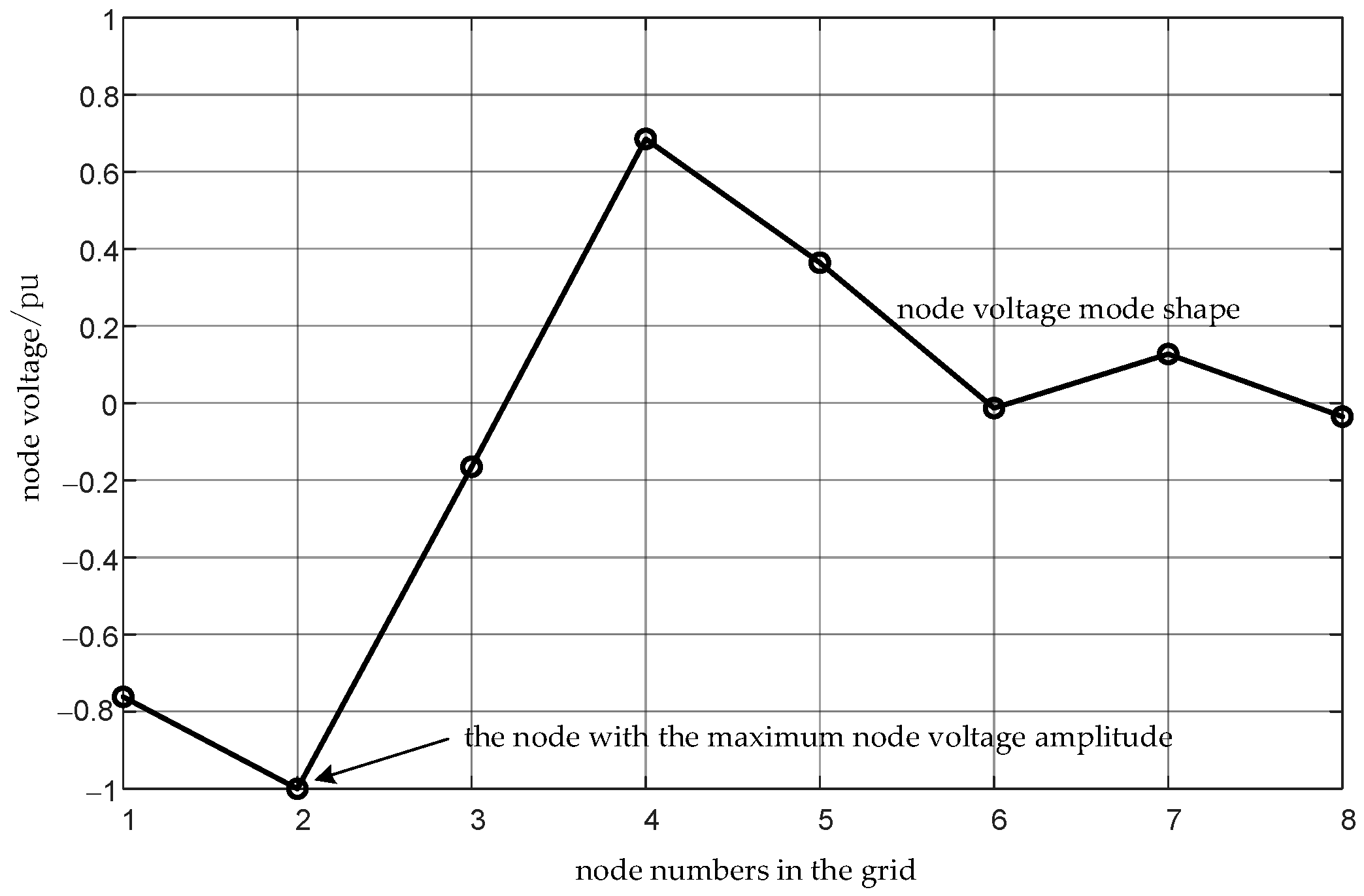
If we set the node voltage mode shape M₁(jω_i) = [m₁ m₂ … m_k … m_n]^T, then |m_j| (j = 1, 2, …, n) is referred to as the node voltage amplitude of node j (in per unit). Note that M₁(jω_i) is a normalized column vector, so the maximum value of |m_j| (j = 1, 2, …, n) is 1. If the k-th element in M₁(jω_i), |m_k| = 1, then the k-th node in the grid is called the node with the maximum node voltage amplitude. Figure 2 shows the node voltage mode shape corresponding to the #3 resonant mode of the benchmark system to be introduced later. The horizontal axis represents the indices of the elements in M₁(jω₃), which simultaneously denote the node numbers in the grid. The vertical axis indicates the values of m_j (j = 1, 2, …, n), representing the amplitude and phase relationship of the node voltages corresponding to the grid node numbers.

According to Equation (15), at the resonance frequency ω_i, the voltage magnitude at the j-th node (j = 1, 2, …, n) in the grid is equal to the product of the absolute value of the j-th element m_j in M₁(jω_i) and the resonant peak voltage |U_mode1(jω_i)|. Obviously, at the resonance frequency ω_i, the voltage magnitude at the node with the maximum nodal voltage amplitude is exactly equal to the resonant peak voltage |U_mode1(jω_i)|. Thus, the resonant peak voltage |U_mode1(jω_i)| can be directly calculated through network analysis, and its value is precisely the voltage magnitude at the node with the maximum nodal voltage amplitude.

Note that the resonant peak voltage |U_mode1(jω_i)| is defined under the assumption of a lossless grid. In this case, according to Equation (14), |U_mode1(jω_i)| = |J_mode1(jω_i)/λ₁(jω_i)| = ∞, i.e., |V_node(jω_i)| = ∞. This implies that all nodal voltages in the grid are infinite. Such a situation is impossible in an actual power grid, as a practical grid inherently possesses damping.

Under the condition that damping exists in the power grid, and by comparing the resonant peak voltage Equations (3) and (6) for the fundamental RLC series resonant circuit and RLC parallel resonant circuit, along with the definition of the modal node injection current vector as given in Equation (11), it is reasonable to infer the following expression for the resonant peak voltage:

$$\left\{\begin{array}{c}\left|U_{\mathrm{mode}1}(\mathrm{j}{\omega }_i)\right|={\displaystyle \frac{1}{{\zeta }_i}}\left|{\underset{\_}{J}}_{\mathrm{mode}1}^{\prime }(\mathrm{j}{\omega }_i)\right|\\ {\underset{\_}{J}}_{\mathrm{mode}1}^{\prime }(\mathrm{j}{\omega }_i)={\underset{\_}{c}}_1(\mathrm{j}{\omega }_i){\underset{\_}{I}}_1(\mathrm{j}{\omega }_i)+{\underset{\_}{c}}_2(\mathrm{j}{\omega }_i){\underset{\_}{I}}_2(\mathrm{j}{\omega }_i)+\cdots +{\underset{\_}{c}}_n(\mathrm{j}{\omega }_i){\underset{\_}{I}}_n(\mathrm{j}{\omega }_i)\end{array}\right.$$

(16)

In Equation (16), ζ_i represents the damping ratio of the i-th resonant mode under damped conditions, J_mode1′ (jω_i) denotes the first element in the modal injection current column vector, I₁(jω_i), I₂(jω_i), …, I_n(jω_i) are the injected currents at each node of the grid, and c₁(jω_i), c₂(jω_i), …, c_n(jω_i) are coefficients dependent on the grid structure and parameters.

Additionally, when the harmonic source frequency is relatively close to the resonance frequency ω_i, the relationship between the node voltage vector V_node(jω_i), the voltage mode shape M₁(jω_i), and the resonant peak voltage |U_mode1(jω_i)| remains applicable. That is, Equation (15) still holds within the neighborhood of ω_i.

The above five components constitute the theoretical framework for the “harmonic amplification” mechanism of wideband oscillations. To verify this mechanism, reveal the fundamental characteristics of wideband oscillations, and explore control strategies for mitigating them, it is imperative to construct a benchmark system.

3. Structure and Parameters of the Benchmark System

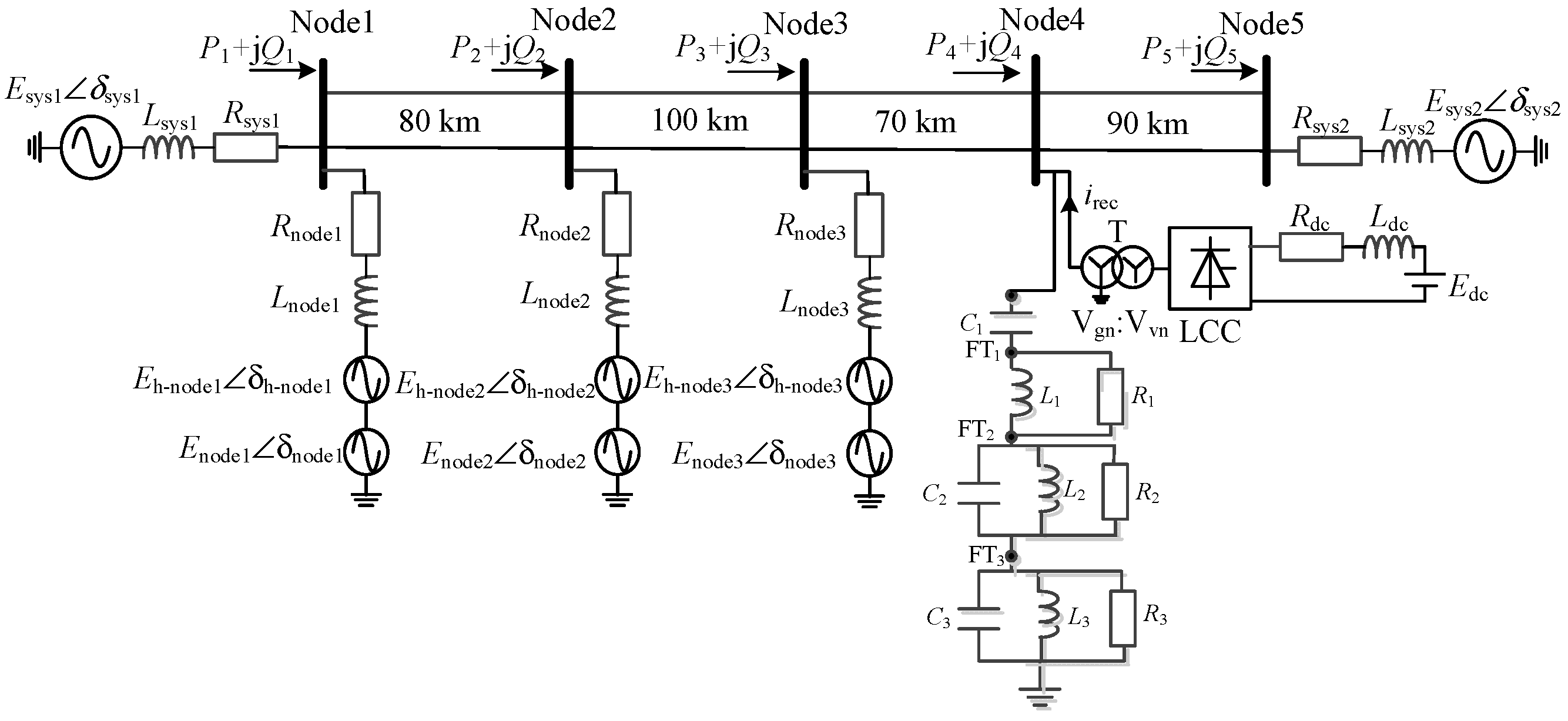
The structure of the benchmark system is shown in Figure 3, representing a scenario where a 50 Hz, 500 kV renewable energy base delivery system supplies power to a DC transmission rectifier load. The 500 kV AC transmission line is divided into four sections, featuring a double-circuit configuration throughout, with five nodes labeled as Node1, Node2, Node3, Node4, and Node5. The sending-end AC system is sys1, and the receiving-end AC system is sys2. Three renewable energy bases are distributed along the transmission line, each represented by its wideband voltage source converter model [11]. The power from these three renewable energy bases is transmitted to a remote location via the DC transmission system. The DC transmission system has a rated voltage of 400 kV, a rated current of 5 kA, and a rated power of 2000 MW. The rectifier station of the DC transmission system is represented by a 6-pulse line-commutated converter (LCC), and the AC bus on the grid side of the LCC is equipped with a triple-tuned filter [10,22], with tuning frequencies of 150.0 Hz, 1200 Hz, and 1850 Hz, respectively. The parameters of each component in the benchmark system are provided in

Table 1. Electrical Parameters of The Single-circuit 500 kV AC Transmission Line.

Electrical Parameters per Unit Length	R (Ω/km)	L (mH/km)	C (μF/km)
Positive sequence/Negative sequence	0.0196	0.8780	0.01313
Zero sequence	0.1522	2.2840	0.009879

,

Table 2. Parameters of Thevenin Equivalent Circuits for AC Systems on Both Sides.

Item	Phase A Equivalent Resistance Rsys (Ω)	Phase A Equivalent Inductance Lsys (mH)	Phase A Equivalent Electromotive Force Magnitude Esys (kV)	Phase A Equivalent Electromotive Force Phase Angle δsys (°)
Sending-end AC system 1	1.25	39.8	408.2483 × 1.01952	11.4492
Receiving-end AC system 2	0.625	19.9	408.2483 × 1.07003	−0.20328

,

Table 3. Model Parameters of Wideband Voltage-Source Converters for Three Renewable Energy Bases.

Item	Node1	Node2	Node3
Phase A equivalent resistance Rnode (Ω)	7.5	3.75	7.5
Phase A equivalent inductance Lnode (mH)	238.7	119.4	238.7
Phase A fundamental-frequency equivalent electromotive force frequency f0 (Hz)	50	50	50
Phase A fundamental-frequency equivalent electromotive force magnitude Enode (kV)	408.2483 × 1.01624	408.2483 × 1.01809	408.2483 × 1.1363
Phase A fundamental-frequency equivalent electromotive force phase angle δnode (°)	19.6573	18.1683	11.8038
Phase A fundamental-frequency equivalent electromotive force phase sequence	Positive sequence	Positive sequence	Positive sequence
Phase A harmonic electromotive force frequency fh_node (Hz)	30	75	160
Phase A harmonic electromotive force magnitude Eh_node (kV)	50	50	50
Phase A harmonic electromotive force phase angle δh_node (°)	0	0	0
Phase A harmonic electromotive force phase sequence	Positive sequence	Negative sequence	Positive sequence

,

Table 4. Parameters of the HVDC transmission system.

Three-Phase Converter Transformer	Rated Capacity (MVA)	Short-Circuit Impedance uk (%)	Grid-Side Rated Voltage Vgn (kV)	Valve-Side Rated Voltage Vvn/(kV)	Grid-Side Tap Position (%)
	2400	18	500	340	98
Rectifier	Structure	Operating condition
	6-pulse LCC	DC voltage 400 kV, DC current 5 kA, firing angle 14.2°
Equivalent DC system	Rated voltage (kV)	Rated current (kA)	Line resistance Rdc (Ω)	Line inductance Ldc (mH)	Inverter-side equivalent EMF Edc (kV)
	400	5	5.4	3000	373

and

Table 5. Parameters of the triple-tuned filter.

Component	Parameter	Component	Parameter	Component	Parameter
R1 (Ω)	1500	R2 (Ω)	400	R3 (Ω)	106
L1 (mH)	8.047	L2 (mH)	126.556	L3 (mH)	1.608
C1 (μF)	1.57929	C2 (μF)	7.29461	C3 (μF)	7.76831

.

4. Calculation of Resonant Modes and Voltage Mode Shapes for the Benchmark System

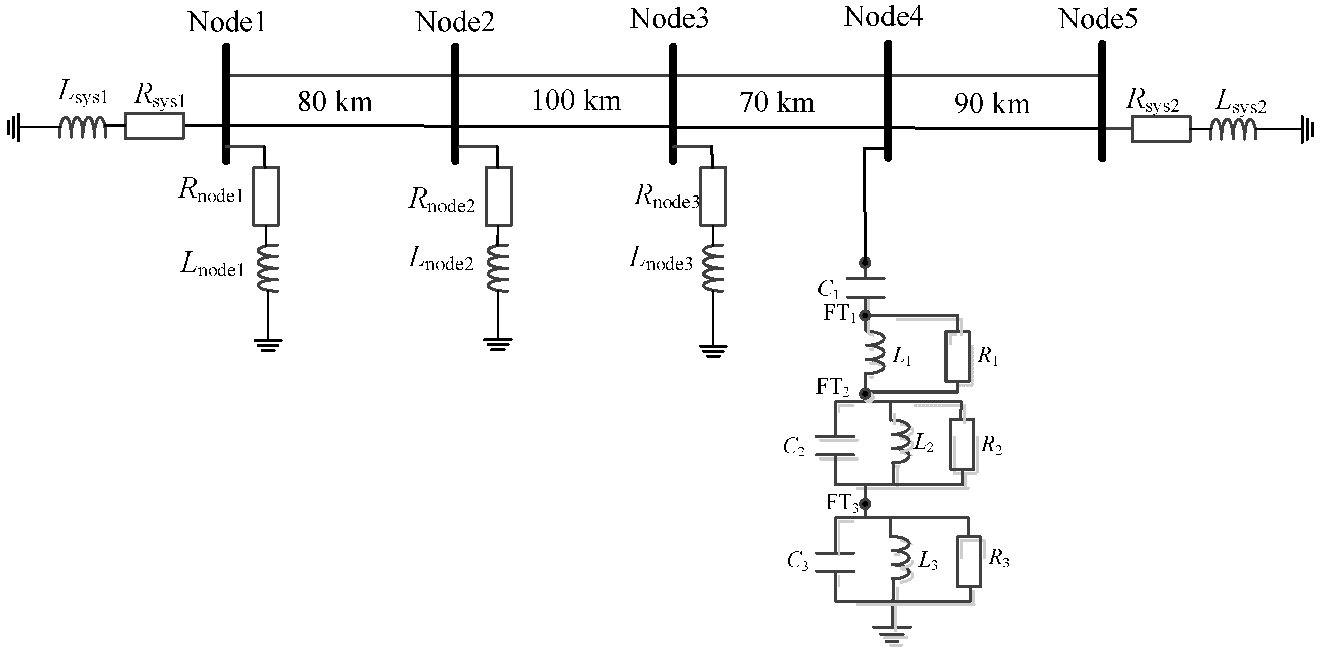
To calculate the resonance modes and voltage mode shapes of the benchmark system shown in Figure 3, it is first necessary to establish the positive-sequence grid impedance model of the system. The positive-sequence grid impedance model is developed based on the following principles: (1) independent voltage sources are replaced by short circuits; (2) independent current sources are replaced by open circuits; (3) LCCs are treated as current-source converters and thus replaced by open circuits. The positive-sequence network impedance model of the benchmark system, established according to the above three principles, is shown in Figure 4.

The s-domain nodal admittance matrix method implemented in two steps [10,22] is employed to calculate the resonance modes and their corresponding node voltage mode shapes of the positive-sequence grid impedance model shown in Figure 4 within the frequency range of 1000 Hz. The calculation results are shown in

Table 6. Resonance modes and node voltage mode shapes of the benchmark system within 1000 Hz range.

Resonance Mode Number		#1	#2	#3
Resonance frequency (Hz)		147.6685	350.4990	632.3371
Damping ratio		0.1470	0.0100	0.0049
node voltage mode shapes	Node1	0.0115	0.4000	−0.7617
	Node2	0.0228	0.7182	−1.0000
	Node3	0.0431	1.0000	−0.1651
	Node4	0.0604	0.9999	0.6853
	Node5	0.0207	0.3815	0.3642
	FT1	−1.0000	0.1693	−0.0127
	FT2	−0.9882	0.2206	0.1274
	FT3	−0.0024	−0.0109	−0.0349

.

As can be seen from Table 6, the benchmark system has a total of three resonance modes within the 1000 Hz frequency range. Resonance mode #1 corresponds to the first resonance frequency point of the triple-tuned filter. From the node voltage mode shape of this resonance mode, it can be observed that the oscillation range corresponding to this mode is mainly confined within the triple-tuned filter. We refer to this type of resonance mode as a local resonance mode. The resonance frequency of resonance mode #2 is 350.4990 Hz, which is very close to the 7th harmonic frequency, and its damping ratio is only 0.01. Therefore, special attention must be paid to the harmonic amplification effect caused by this mode. Furthermore, from the node voltage mode shape of resonance mode #2, it can be seen that the oscillation range corresponding to this mode is system-wide, with the maximum node voltage amplitude occurring at Node 3 and Node 4. The resonance frequency of resonance mode #3 is 632.3371 Hz, which is close to the 13th harmonic frequency, and its damping ratio is only 0.0049. The harmonic amplification effect caused by this mode also requires special attention. From the node voltage mode shape of resonance mode #3, it can be observed that the oscillation range corresponding to this mode is also system-wide, with the maximum node voltage amplitude occurring at Node 2.

Next, the electromagnetic transient simulation method will be used to quantitatively investigate the harmonic amplification characteristics corresponding to resonance modes #2 and #3.

5. Time-Domain Waveform Presentation

The frequencies of the excitation sources in the benchmark system shown in Figure 3 are 50 Hz, 30 Hz, 75 Hz, and 160 Hz, respectively. The greatest common divisor of these four frequencies is 5 Hz, which means that the minimum period of the physical quantities in the benchmark system is 200 ms. Therefore, only a waveform segment within a 200 ms interval is presented for the time-domain waveform display. Since electromagnetic transient simulations require a certain amount of time to transition from the initial state to a steady state, the following time-domain waveform display shows the waveform from 5 s to 5.2 s.

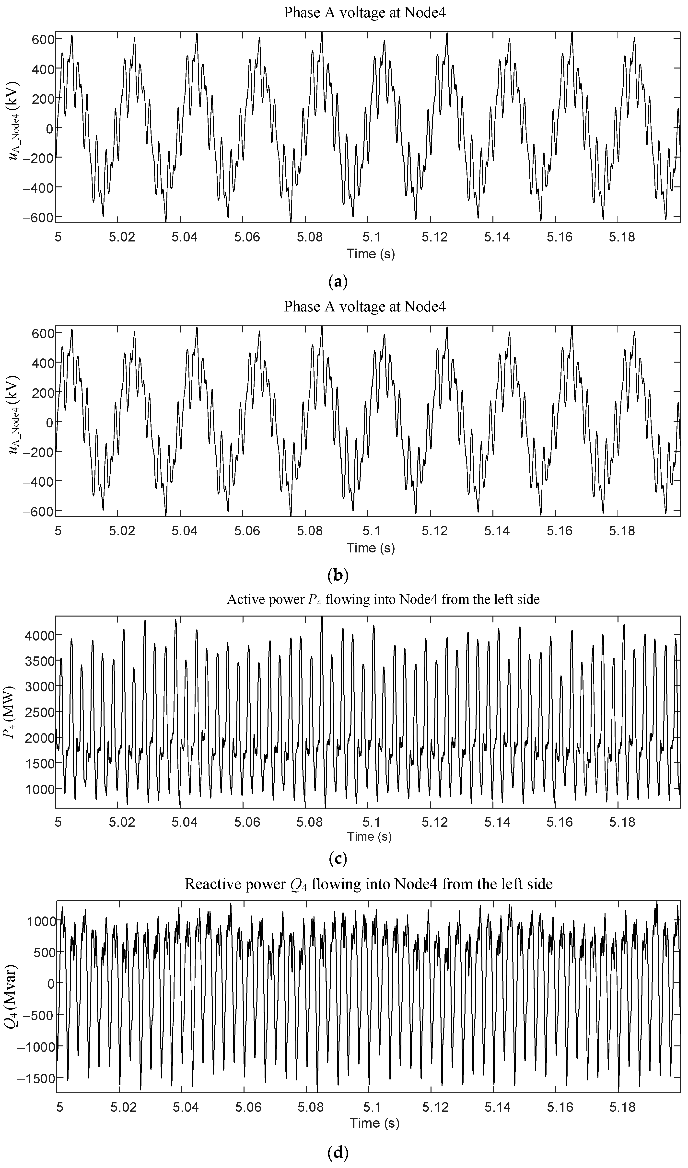
Taking the electrical quantities at Node4 as an example for the time-domain waveform displays, Figure 5 shows the voltage at Node4, the total current of the double-circuit transmission lines flowing into Node4 from the left side, as well as the total active power and total reactive power waveforms of these double-circuit transmission lines flowing into Node4 from the left side. From the active power waveform in Figure 5, it can be observed that the average power is approximately 2000 MW, while the peak power exceeds 4000 MW, indicating that the power oscillation amplitude surpasses 2000 MW. Clearly, a severe power oscillation phenomenon occurs at Node4. However, the power oscillation waveform in Figure 5 is severely distorted, making it difficult to discern the frequency components of the power oscillation from the time-domain waveform. Nevertheless, it is certain that the frequency spectrum contained in the oscillating power is wide, hence it is referred to as wideband power oscillation. From the phase A voltage waveform in Figure 5, it can be seen that the voltage peak exceeds 600 kV, whereas the rated phase voltage amplitude at Node4 is 408.2483 kV, indicating an overvoltage phenomenon exceeding 1.46 times the rated value. In summary, from the time-domain waveforms in Figure 5, we observe the wideband power oscillation phenomenon and overvoltage phenomenon resulting from harmonic amplification.

6. Harmonic Decomposition Results and Characteristic Analysis of Current Waveforms

The harmonic decomposition [23] of the current waveforms at the main nodes along the transmission lines of the benchmark system shown in Figure 3 is performed, and the obtained results are presented in

Table 7. Harmonic decomposition results of currents at main nodes of the transmission line.

Row Number	Harmonic Frequency (Hz)	LCC Harmonic Current Source irec (A)	Harmonic Current Amplitude (A)
			Node1	Node2	Node3	Node4	Node5
1	30 (source)	14.60	685	298.44	158.27	116.87	109.60
2	50 (fund.)	3752.96	197.97	975.97	2571.21	3392.74	1087.02
3	60	11.32	1.82	2.09	3.24	4.36	7.20
4	70	15.54	2.53	2.89	4.44	5.94	9.92
5	75 (source)	40.73	356.92	406.39	254.30	186.12	208.06
6	125	26.60	5.07	5.52	7.94	10.12	18.88
7	140	9.02	1.83	1.95	2.74	3.42	6.67
8	160 (source)	9.93	64.61	67.19	90.25	93.59	119.16
9	175	44.53	10.30	10.45	13.53	15.82	35.43
10	225	18.50	5.93	5.45	5.92	5.87	18.28
11	250 (5th)	385.38	157.12	135.46	129.05	109.52	451.82
12	270	16.25	8.55	6.95	5.75	3.93	23.08
13	330	3.90	8.59	5.55	1.75	2.02	18.23
14	350 (7th)	52.39	698.22	407.78	32.15	313.31	1336.80
15	360	8.56	41.18	22.74	1.73	22.68	74.53
16	370	16.35	41.55	21.58	4.94	26.96	70.78
17	375	43.69	90.58	45.54	14.36	63.11	149.47
18	475	37.74	24.24	3.36	21.77	33.38	13.65
19	550 (11th)	217.25	166.05	28.04	219.53	243.60	36.41
20	570	10.73	10.02	2.55	14.10	14.27	4.13
21	630	1.71	20.62	10.66	32.62	23.50	19.33
22	650 (13th)	240.63	608.99	369.17	980.72	607.03	663.72
23	660	5.59	8.95	5.83	14.48	8.21	10.39
24	670	7.82	9.04	6.30	14.68	7.53	11.12
25	675	22.18	22.69	16.29	36.83	17.90	28.60
26	775	13.74	3.92	4.57	5.58	1.01	6.61
27	850 (17th)	170.75	35.20	52.50	36.03	38.36	58.33
28	950 (19th)	107.71	24.56	46.54	5.28	47.06	23.10

. For the benchmark system, with the exception of the three harmonic voltage sources at 30 Hz, 75 Hz, and 160 Hz, all harmonic sources at other frequencies are generated by the LCC, and the harmonic sources produced by the LCC are characterized as current sources.

In Table 7, apart from the fundamental frequency and the harmonic currents at 30 Hz, 75 Hz, and 160 Hz, the harmonic currents at other frequencies are all caused by the harmonic current source i_rec. Therefore, for the harmonic current frequencies caused by i_rec, if the harmonic current flowing through any point on the line is greater than i_rec, it can be considered that harmonic current amplification has occurred. Upon examining the rows in Table 7, it is found that harmonic current amplification occurs in Rows 11 to 17 and Rows 19 to 25, i.e., within the frequency ranges of 250–375 Hz and 550–675 Hz. According to the calculation results of resonance modes and voltage mode shapes in Table 6, the harmonic amplification frequency range of 250–375 Hz corresponds to the resonance frequency of 350.4990 Hz for resonance mode #2, and the harmonic amplification frequency range of 550–675 Hz corresponds to the resonance frequency of 632.3371 Hz for resonance mode #3.

Then, what is the relationship between the harmonic current amplification effect and the node voltage mode shapes? We focus on examining the distribution characteristics of the 350 Hz harmonic current, which is closest to the resonance frequency of 350.4990 Hz of mode #2, and the 630 Hz harmonic current, which is closest to the resonance frequency of 632.3371 Hz of mode #3. The comparative relationship between the harmonic current amplification effect and the node voltage mode shapes is shown in

Table 8. Relationship between node voltage mode shape and harmonic current amplification effect.

Frequency (Hz)	Item	irec	Node1	Node2	Node3	Node4	Node5
350.4990	node voltage mode shape	-	0.4000	0.7182	1.0000	0.9999	0.3815
350	Harmonic current (A)	52.39	698.22	407.78	32.15	313.31	1336.80
350	Harmonic current amplification factor	-	13.3	7.8	0.61	5.9	25.5
632.3371	node voltage mode shape	-	−0.7617	−1.0000	−0.1651	0.6853	0.3642
630	Harmonic current (A)	1.71	20.62	10.66	32.62	23.50	19.33
630	Harmonic current amplification factor	-	12.1	6.2	19.1	13.7	11.2

.

It can be seen from Table 8 that the node with the maximum node voltage amplitude in the node voltage mode shape corresponds to the smallest harmonic current amplification factor. For example, for the 350 Hz harmonic current, Node3 is the node with the maximum node voltage amplitude, and its harmonic current amplification factor is the smallest among the five listed nodes. Conversely, the node with the minimum node voltage amplitude in the node voltage mode shape corresponds to the largest harmonic current amplification factor. For instance, for the 350 Hz harmonic current, Node5 is the node with the minimum node voltage amplitude, and its harmonic current amplification factor is the largest among the five listed nodes, reaching 25.5. The same result is observed for the 630 Hz harmonic current. Thus, it is evident that there is a definite relationship between the harmonic current amplification effect and the node voltage mode shapes: the harmonic current amplification factor is smallest at the node with the maximum node voltage amplitude, and largest at the node with the minimum node voltage amplitude.

7. Harmonic Decomposition Results and Characteristic Analysis of Voltage Waveforms

The harmonic decomposition of the voltage waveforms at the main nodes along the transmission lines of the benchmark system shown in Figure 3 is performed, and the obtained results are presented in

Table 9. Voltage harmonic decomposition results at the main nodes of the transmission line.

Frequency (Hz)	Harmonic Voltage Amplitude (kV)
	Node1	Node2	Node3	Node4	Node5
30 (Source at Node1)	5.21	3.23	1.91	1.24	0.42
50 (Fundamental)	417.11	417.85	419.35	414.83	430.13
75 (Source at Node2)	6.71	13.53	8.42	5.80	1.96
160 (Source at Node3)	2.59	5.12	9.58	6.93	2.38
250 (5th)	9.82	18.75	31.62	39.50	14.12
350 (7th)	61.11	109.77	153.09	153.39	58.5
360	3.71	6.61	9.0	8.73	3.35
370	3.84	6.80	9.02	8.45	3.27
375	8.49	14.97	19.59	18.01	7.01
550 (11th)	22.83	33.70	19.45	5.33	2.50
630	3.25	4.28	0.76	2.88	1.52
650 (13th)	98.98	126.33	9.26	98.50	53.94
850 (17th)	7.48	6.17	6.86	7.15	6.20
950 (19th)	5.84	3.41	6.35	2.20	2.74

.

First, we examine the harmonic voltage distribution caused by the three harmonic voltage sources at 30 Hz, 75 Hz, and 160 Hz. The 30 Hz harmonic voltage source is connected to Node1, and the 30 Hz harmonic voltage at Node1 is the largest; the 75 Hz harmonic voltage source is connected to Node2, and the 75 Hz harmonic voltage at Node2 is the largest; the 160 Hz harmonic voltage source is connected to Node3, and the 160 Hz harmonic voltage at Node3 is the largest. This indicates that there are no signs of harmonic amplification at the frequencies of 30 Hz, 75 Hz, and 160 Hz.

It can be observed from Table 9 that the harmonic voltages are largest at the frequencies of 350 Hz and 650 Hz, with maximum harmonic voltages reaching 153.39 kV and 126.33 kV, respectively. These two frequencies share common characteristics: (1) They are close to resonance frequencies—350 Hz is near the 350.4990 Hz resonance frequency, and 650 Hz is near the 632.3371 Hz resonance frequency. (2) They belong to the characteristic harmonic current frequencies of the LCC, and the harmonic current values are relatively large. The combined effect of these two conditions results in the amplification of harmonic voltages at the corresponding frequencies. Referring to Table 7, it can be found that the harmonic current value of the LCC at the characteristic frequency of 250 Hz is 385.38 A, while at the characteristic frequency of 350 Hz, it is 52.39 A. The latter is much smaller than the former, but the harmonic voltage value caused by the latter is significantly larger (as can be seen from Table 9, the maximum harmonic voltage at 250 Hz is 39.50 kV). The reason why a smaller harmonic current at 350 Hz leads to a larger harmonic voltage is the presence of a resonance frequency point near 350 Hz. This result also holds true for the characteristic harmonic current at 650 Hz. Thus, it is evident that deviation of characteristic harmonic frequencies from resonance frequencies is beneficial for avoiding harmonic amplification.

Next, we focus on examining the relationship between harmonic voltage distribution and node voltage mode shapes. The analysis selects the harmonic voltage distributions at 350 Hz and 375 Hz, which are closest to the #2 resonance frequency of 350.4990 Hz, and at 630 Hz and 650 Hz, which are closest to the #3 resonance frequency of 632.3371 Hz. It should be noted that the harmonic voltage at 630 Hz is very small, which may have a certain impact on calculation accuracy. The analysis results are shown in

Table 10. Relationship between node voltage mode shape and harmonic voltage distribution.

Frequency (Hz)	Item	Node1	Node2	Node3	Node4	Node5
350.4990	node voltage mode shape	0.4000	0.7182	1.0000	0.9999	0.3815
350	Harmonic voltage (kV)	61.11	109.77	153.09	153.39	58.5
350	Resonant peak voltage (kV)	152.8	152.8	153.1	153.4	153.3
375	Harmonic voltage (kV)	8.49	14.97	19.59	18.01	7.01
375	Resonant peak voltage (kV)	21.2	20.8	19.59	18.01	18.4
632.3371	node voltage mode shape	−0.7617	−1.0000	−0.1651	0.6853	0.3642
630	Harmonic voltage (kV)	3.25	4.28	0.76	2.88	1.52
630	Resonant peak voltage (kV)	4.27	4.28	4.6	4.20	4.17
650	Harmonic voltage (kV)	98.98	126.33	9.26	98.50	53.94
650	Resonant peak voltage (kV)	129.9	126.3	56.1	143.7	148

. From Table 10, it can be seen that the resonant peak voltages calculated in the vicinity of the resonance frequencies (e.g., 350 Hz in the neighborhood of the #2 resonance frequency and 630 Hz in the neighborhood of the #3 resonance frequency) are approximately constant. This finding is consistent with point 5 in the theoretical framework of the “harmonic amplification” mechanism of wideband oscillation discussed in Section 1.

Additionally, it can be observed that the resonant peak voltage is primarily related to three factors: (1) the resonance frequency; (2) the magnitude of the harmonic source; (3) the location of the harmonic source. Comparing the resonant peak voltages at 350 Hz and 630 Hz in Table 10, the location of the harmonic source is the same, while the resonance frequency and the magnitude of the harmonic source differ. The harmonic current source value at 350 Hz is 52.39 A, whereas the harmonic current source value at 630 Hz, as shown in Table 7, is 1.71 A. Consequently, the resonant peak voltage at 350 Hz is 153.1 kV, while at 630 Hz it is 4.28 kV. If we calculate the resonant peak voltage under the excitation of a unit harmonic current, it is 2.89 kV at 350 Hz and 2.50 kV at 630 Hz. The difference between these two values indicates that the resonance frequency is indeed a factor influencing the resonant peak voltage. Clearly, a larger resonant peak voltage signifies a more severe harmonic amplification effect.

Based on the above analysis, it is found that the key factors determining the harmonic amplification effect at various nodes of the power grid are fourfold: resonance frequency, damping ratio, node voltage mode shape, and resonant peak voltage. The first three factors are determined by the grid topology and the parameters of grid components, and they are relatively fixed characteristics with little correlation to the power generation output and load level of the grid. However, the resonant peak voltage is not only related to the grid topology and component parameters but is also closely associated with the distribution and magnitude of harmonic sources within the grid. Its theoretical expression is shown in Equation (16). The distribution and magnitude of harmonic sources are closely related to the distribution and output of renewable energy sources, as well as the load level and its distribution in the grid, with the latter exhibiting strong randomness and volatility. Consequently, the resonant peak voltage continuously varies with the operating conditions of the power grid, and thus the harmonic amplification effect also changes dynamically with the grid’s operating conditions.

Furthermore, the above results indicate that analyzing the resonance structure of the power grid—including resonance frequency, damping ratio, and node voltage mode shape—using the s-domain nodal admittance matrix method based on the positive-sequence grid model is effective. These results can be mutually verified with electromagnetic transient simulation results based on three-phase models.

8. Results of Harmonic Decomposition of Power Waveform and Its Characteristic Analysis

8.1. Basic Characteristics of Oscillatory Power Components in Three-Phase AC Systems

Before analyzing the harmonic decomposition results of the power waveform, the relationship between oscillatory power and oscillatory voltage and current in a three-phase AC system will first be derived. The fundamental frequency voltage and current of the three-phase AC system are set as positive sequence components, while the oscillatory voltage and current of the three-phase AC system are considered as positive sequence and negative sequence components, respectively. The expressions for three-phase voltage and current containing positive sequence oscillatory voltage and current are shown in Equations (17) and (18); the expressions for three-phase voltage and current containing negative sequence oscillatory voltage and current are shown in Equations (19) and (20). In Equations (17)–(20), u_a, u_b, u_c and i_a, i_b, i_c represent the three-phase AC voltage and current containing oscillatory components; U₁, ω₀, and δ₀ represent the amplitude, angular frequency, and initial phase angle of the three-phase fundamental frequency voltage; I₁ and θ₀ represent the amplitude and initial phase angle of the three-phase fundamental frequency current; U_osc⁺, ω_osc⁺, and φ⁺ represent the amplitude, angular frequency, and initial phase angle of the three-phase positive sequence oscillatory voltage; I_osc⁺ and ϕ⁺ represent the amplitude and initial phase angle of the three-phase positive sequence oscillatory current; U_osc⁻, ω_osc⁻, and φ⁻ represent the amplitude, angular frequency, and initial phase angle of the three-phase negative sequence oscillatory voltage; I_osc⁻ and ϕ⁻ represent the amplitude and initial phase angle of the three-phase negative sequence oscillatory current.

$$\left\{\begin{array}{c}{u}_{\mathrm{a}}=U_1\sin ({\omega }_{0}t+{\delta }_0)+U_{\mathrm{osc}}^{+}\sin ({\omega }_{\mathrm{osc}}^{+}t+{\phi }^{+})\\ u_{\mathrm{b}}=U_1\sin ({\omega }_{0}t+{\delta }_0-2\pi /3)+U_{\mathrm{osc}}^{+}\sin ({\omega }_{\mathrm{osc}}^{+}t+{\phi }^{+}-2\pi /3)\\ u_{\mathrm{c}}=U_1\sin ({\omega }_{0}t+{\delta }_0+2\pi /3)+U_{\mathrm{osc}}^{+}\sin ({\omega }_{\mathrm{osc}}^{+}t+{\phi }^{+}+2\pi /3)\end{array}\right.$$

(17)

$$\left\{\begin{array}{c}{i}_{\mathrm{a}}=I_1\sin ({\omega }_{0}t+{\theta }_0)+I_{\mathrm{osc}}^{+}\sin ({\omega }_{\mathrm{osc}}^{+}t+{\varphi }^{+})\\ i_{\mathrm{b}}=I_1\sin ({\omega }_{0}t+{\theta }_0-2\pi /3)+I_{\mathrm{osc}}^{+}\sin ({\omega }_{\mathrm{osc}}^{+}t+{\varphi }^{+}-2\pi /3)\\ i_{\mathrm{c}}=I_1\sin ({\omega }_{0}t+{\theta }_0+2\pi /3)+I_{\mathrm{osc}}^{+}\sin ({\omega }_{\mathrm{osc}}^{+}t+{\varphi }^{+}+2\pi /3)\end{array}\right.$$

(18)

$$\left\{\begin{array}{c}{u}_{\mathrm{a}}=U_1\sin ({\omega }_{0}t+{\delta }_0)+U_{\mathrm{osc}}^{-}\sin ({\omega }_{\mathrm{osc}}^{-}t+{\phi }^{-})\\ u_{\mathrm{b}}=U_1\sin ({\omega }_{0}t+{\delta }_0-2\pi /3)+U_{\mathrm{osc}}^{-}\sin ({\omega }_{\mathrm{osc}}^{-}t+{\phi }^{-}+2\pi /3)\\ u_{\mathrm{c}}=U_1\sin ({\omega }_{0}t+{\delta }_0+2\pi /3)+U_{\mathrm{osc}}^{-}\sin ({\omega }_{\mathrm{osc}}^{-}t+{\phi }^{-}-2\pi /3)\end{array}\right.$$

(19)

$$\left\{\begin{array}{c}{i}_{\mathrm{a}}=I_1\sin ({\omega }_{0}t+{\theta }_0)+I_{\mathrm{osc}}^{-}\sin ({\omega }_{\mathrm{osc}}^{-}t+{\varphi }^{-})\\ i_{\mathrm{b}}=I_1\sin ({\omega }_{0}t+{\theta }_0-2\pi /3)+I_{\mathrm{osc}}^{-}\sin ({\omega }_{\mathrm{osc}}^{-}t+{\varphi }^{-}+2\pi /3)\\ i_{\mathrm{c}}=I_1\sin ({\omega }_{0}t+{\theta }_0+2\pi /3)+I_{\mathrm{osc}}^{-}\sin ({\omega }_{\mathrm{osc}}^{-}t+{\varphi }^{-}-2\pi /3)\end{array}\right.$$

(20)

When the phase sequence of the oscillatory voltage and current in the power grid is positive, the expression for the three-phase instantaneous active power is

$$\begin{array}{l}{p}_{\mathrm{abc}}=u_{\mathrm{a}}{i}_{\mathrm{a}}+u_{\mathrm{b}}{i}_{\mathrm{b}}+u_{\mathrm{c}}{i}_{\mathrm{c}}={\displaystyle \frac{3U_1{I}_1}{2}}\cos ({\delta }_0-{\theta }_0)+{\displaystyle \frac{3U_{\mathrm{osc}}^{+}{I}_{\mathrm{osc}}^{+}}{2}}[\cos ({\phi }^{+}-{\varphi }^{+})\\ +{\displaystyle \frac{3U_1{I}_{\mathrm{osc}}^{+}}{2}}\cos [({\omega }_0-{\omega }_{\mathrm{osc}}^{+})t+{\delta }_0-{\varphi }^{+}]+{\displaystyle \frac{3U_{\mathrm{osc}}^{+}{I}_1}{2}}\cos [({\omega }_0-{\omega }_{\mathrm{osc}}^{+})t+{\phi }^{+}-{\theta }_0]\end{array}$$

(21)

When the phase sequence of the oscillatory voltage and current in the power grid is negative, the expression for the three-phase instantaneous active power is

$$\begin{array}{l}{p}_{\mathrm{abc}}=u_{\mathrm{a}}{i}_{\mathrm{a}}+u_{\mathrm{b}}{i}_{\mathrm{b}}+u_{\mathrm{c}}{i}_{\mathrm{c}}={\displaystyle \frac{3U_1{I}_1}{2}}\cos ({\delta }_0-{\theta }_0)+{\displaystyle \frac{3U_{\mathrm{osc}}^{-}{I}_{\mathrm{osc}}^{-}}{2}}\cos ({\phi }^{-}-{\varphi }^{-})\\ -{\displaystyle \frac{3U_1{I}_{\mathrm{osc}}^{-}}{2}}\cos [({\omega }_0+{\omega }_{\mathrm{osc}}^{-})+{\delta }_0+{\varphi }^{-}]-{\displaystyle \frac{3U_{\mathrm{osc}}^{-}{I}_1}{2}}\cos [({\omega }_0+{\omega }_{\mathrm{osc}}^{-})t+{\phi }^{-}+{\theta }_0]\end{array}$$

(22)

From Equations (21) and (22), it can be seen that when the three-phase AC system contains oscillatory voltage and current beyond the fundamental frequency, the three-phase instantaneous active power is no longer a constant but a quantity that contains both a DC component and an oscillatory component, varying over time. If f_power is used to represent the oscillation frequency of the oscillatory component in the three-phase instantaneous active power, with the frequency corresponding to ω₀ denoted as f₀, the frequency corresponding to ω_osc⁺ denoted as f_osc⁺, and the frequency corresponding to ω_osc⁻ denoted as f_osc⁻, then according to Equations (21) and (22), f_power satisfies the following relationship:

$$f_{\mathrm{power}}=\left\{\begin{array}{c}\left|f_{\mathrm{osc}}^{+}-f_0\right|, \mathrm{when} \mathrm{the} \mathrm{oscillatory} \mathrm{voltage} \mathrm{and} \mathrm{current} \mathrm{are} \mathrm{of} \mathrm{positive} \mathrm{sequence}\\ f_{\mathrm{osc}}^{-}+f_0, \mathrm{when} \mathrm{the} \mathrm{oscillatory} \mathrm{voltage} \mathrm{and} \mathrm{current} \mathrm{are} \mathrm{of} \mathrm{negative} \mathrm{sequence}\end{array}\right.$$

(23)

Traditionally, power system oscillations are described using the oscillation frequency f_power of the three-phase instantaneous active power. For instance, low-frequency oscillations typically refer to power oscillations where f_power is less than 2.5 Hz, whereas subsynchronous oscillations generally refer to power oscillations where f_power is between 5 and 45 Hz. Given the known power oscillation frequency f_power, how can we derive the oscillation frequency of the voltage and current in the grid? This question is evidently the inverse problem of Equation (23).

From Equation (23), the following two points can be derived:

(1)

If the power oscillation frequency lies within the subsynchronous frequency range, i.e., f_power < f₀, then the voltage and current in the grid must be positive-sequence quantities. Moreover, their oscillation frequency can be expressed by the following formula:

$$f_{\mathrm{osc}}^{+}=f_0\pm f_{\mathrm{power}}, \mathrm{when} f_{power}<f_0$$

(24)

For example, if f_power = 20 Hz, then the oscillation frequency of the voltage and current in the grid could be either 30 Hz or 70 Hz. The specific frequency needs to be determined through actual measurement of the voltage and current quantities.

(2)

If the power oscillation frequency exceeds the fundamental frequency, i.e., f_power > f₀, then determining the oscillation frequency of the voltage and current in the network is relatively straightforward, as shown in the following formula:

$$\left\{\begin{array}{c} f_{\mathrm{osc}}^{+}=f_{\mathrm{power}}+f_0, \mathrm{for} \mathrm{positive} \mathrm{sequence} \mathrm{oscillatory} \mathrm{voltage} \mathrm{and} \mathrm{current} \\ f_{\mathrm{osc}}^{-}=f_{\mathrm{power}}-f_0 , \mathrm{for} \mathrm{negative} \mathrm{sequence} \mathrm{oscillatory} \mathrm{voltage} \mathrm{and} \mathrm{current}\end{array}\right.$$

(25)

For example, if f_power = 300 Hz, then when the voltage and current in the grid are of a positive sequence, their oscillation frequency is 350 Hz; when the voltage and current in the grid are of a negative sequence, their oscillation frequency is 250 Hz.

8.2. Harmonic Decomposition Results of Power Waveforms in the Benchmark System and Their Characteristic Analysis

Harmonic decomposition is performed on the active power waveforms at the main nodes along the transmission line of the benchmark system in Figure 3, and the results obtained are shown in

Table 11. Active power harmonic decomposition results.

Row Number	fpower (Hz)	Active Power Amplitude (MW)
		P1	P2	P3	P4	P5
1	0	107.52	608.60	1605.98	2099.88	65.39
2	20	426.97	188.74	102.95	75.54	70.04
3	110	38.99	40.81	60.13	72.22	76.36
4	125	228.62	256.91	165.33	127.59	144.90
5	280	12.21	12.17	10.10	6.64	12.87
6	300	465.62	370.73	899.69	1083.62	1088.45
7	320	61.47	61.93	70.36	75.54	63.92
8	410	28.27	18.74	34.62	54.57	45.81
9	425	84.02	69.28	149.17	154.11	93.40
10	475	17.63	23.13	11.19	5.45	4.32
11	580	28.13	11.27	21.60	22.98	16.84
12	600	427.45	322.38	678.59	679.03	561.50
13	620	94.34	59.49	13.95	31.72	9.85
14	710	12.10	6.51	9.21	17.08	9.02
15	725	47.95	61.99	18.63	58.06	27.13
16	900	47.49	48.29	91.45	97.50	34.47

.

In Table 11, the oscillatory power component with f_power of 20 Hz is generated by the 30 Hz positive-sequence harmonic voltage source and the 30 Hz positive-sequence harmonic current source (LCC). The oscillatory power component with f_power of 110 Hz is generated by the 160 Hz positive-sequence harmonic voltage source and the 160 Hz positive-sequence harmonic current source (LCC). The oscillatory power component with f_power of 125 Hz is generated by the 75 Hz negative-sequence harmonic voltage source and the 75 Hz negative-sequence harmonic current source (LCC). The oscillatory power component with f_power of 300 Hz is generated by the 5th (negative-sequence) characteristic harmonic current and the 7th (positive-sequence) characteristic harmonic current of the LCC. The oscillatory power component with f_power of 600 Hz is generated by the 11th (negative-sequence) characteristic harmonic current and the 13th (positive-sequence) characteristic harmonic current of the LCC. The oscillatory power component with f_power of 900 Hz is generated by the 17th (negative-sequence) characteristic harmonic current and the 19th (positive-sequence) characteristic harmonic current of the LCC. The oscillatory power components with f_power equal to the remaining frequencies are generated by the non-characteristic harmonic currents of the LCC. It can be observed from Table 11 that for the benchmark system shown in Figure 3, the frequency components of power oscillations are very numerous, indeed exhibiting the characteristics of wideband oscillations.

From Table 11, it can be seen that the maximum value of the oscillatory power component at 300 Hz reaches 1088.45 MW, and the maximum value of the oscillatory power component at 600 Hz reaches 679.03 MW, while the active power transmitted by the transmission line is approximately 2000 MW, indicating that the benchmark system shown in Figure 3 has experienced a severe wideband power oscillation issue. Investigating the causes of the wideband power oscillation, it is evident that the harmonic amplification at 350 Hz and 650 Hz is the decisive factor. The reasons for the occurrence of harmonic amplification are mainly two. The first reason is the presence of numerous harmonic sources in the power grid; the second reason is the occurrence of resonance in the power grid, with the resonance frequency being close to the frequency of the larger harmonic sources. Therefore, to suppress wideband power oscillations, on the one hand, it is necessary to eliminate harmonic sources in the power grid as much as possible; on the other hand, the primary system of the power grid needs to be modified so that the resonant structure of the grid is less prone to harmonic amplification effects. Furthermore, the above results also indicate that it is infeasible to directly determine the resonance frequency of the system through the frequency of the oscillatory power component, because one oscillatory power component frequency corresponds to two possible resonance frequencies.

Next, we focus on examining the relationship between the numerical distribution of oscillatory power components and the node voltage mode shapes. The 300 Hz oscillatory power component, most relevant to the #2 resonance frequency of 350.4990 Hz, and the 600 Hz oscillatory power component, most relevant to the #3 resonance frequency of 632.3371 Hz, are selected for analysis. The comparative results are shown in

Table 12. The relationship between the node voltage mode shapes and the numerical distribution of the oscillatory power components.

Freq. (Hz)	Item	Node1 P1	Node2 P2	Node3 P3	Node4 P4	Node5 P5
350.4990	Node voltage mode shape	0.4000	0.7182	1.0000	0.9999	0.3815
300	Oscillatory power component (MW)	465.62	370.73	899.69	1083.62	1088.45
632.3371	Node voltage mode shape	−0.7617	−1.0000	−0.1651	0.6853	0.3642
600	Oscillatory power component (MW)	427.45	322.38	678.59	679.03	561.50

. It can be observed from Table 12 that there is no definite relationship between the numerical distribution of the oscillatory power components and the node voltage mode shapes. This result indicates that it is infeasible to determine the node voltage mode shapes based on the numerical distribution of the oscillatory power components.

Next, we discuss the possibility of determining the location of harmonic sources based on the numerical distribution of oscillatory power components according to the results in Table 11. The second row in Table 11 corresponds to the oscillatory power component with f_power of 20 Hz. The power P₁ corresponding to Node1 has the largest value, and the main harmonic source is the 30 Hz harmonic voltage source connected to Node1. It seems feasible to determine the harmonic source location based on the position of the maximum value. However, the third row in Table 11 corresponds to the oscillatory power component with f_power of 110 Hz. The primary excitation source for this oscillatory power component is the 160 Hz harmonic voltage source connected to Node3, but the power P₃ corresponding to Node3 is not the largest; instead, the power P₅ corresponding to Node5, which has no harmonic source connected, has the largest value. This disproves the idea of determining the harmonic source location based on the magnitude of the oscillatory power component. In Table 11, the relationship between the numerical distribution corresponding to the oscillatory power components with f_power of 300 Hz and 600 Hz and the locations of harmonic sources also does not satisfy the idea that the oscillatory power component value at the node where the harmonic source is connected is the largest. It can be seen that the idea of determining the location of harmonic sources based on the numerical distribution of oscillatory power components is infeasible.

Additionally, in practical engineering, the measurement error of power meters is about 1%. The maximum instantaneous power value in Table 11 exceeds 4000 MW, making power values below 40 MW difficult to distinguish using power meters. The usable numerical distributions of oscillatory power components in Table 11 are primarily at 20 Hz, 125 Hz, 300 Hz, and 600 Hz.

From the analysis results of the benchmark system, it can be seen that determining the harmonic sources of wideband power oscillations is considerably challenging, and this is a matter of particular concern in practical engineering.

9. Conclusions

This paper constructs a benchmark system for verifying the “harmonic amplification” mechanism of wideband oscillations. Through the characteristic analysis of this benchmark system, the following results are obtained.

(1)

Due to the modulation effect of power electronic devices on background harmonics, the frequency spectrum distribution of harmonic sources in the power grid is very extensive. It is reasonable to describe power electronic devices using a wideband voltage source converter model or a wideband current source converter model.

(2)

The electromagnetic transient simulation results in this paper demonstrate the applicability of analyzing the harmonic amplification effect based on the positive sequence grid model.

(3)

The external manifestations of harmonic amplification are wideband power oscillations, overvoltages, and waveform distortion. The four key elements determining the harmonic amplification effect are the resonance frequency, damping ratio, node voltage mode shape, and resonance peak voltage. Among these, the first three elements are determined by the grid topology and grid component parameters, have little correlation with the power generation output and load level of the grid, and are relatively fixed characteristics. The resonance peak voltage is closely related to the distribution and magnitude of harmonic sources and therefore is closely related to the output level and distribution of renewable energy sources as well as the load level and distribution of the grid, exhibiting randomness and volatility.

(4)

The first three elements corresponding to the harmonic amplification effect—the resonance frequency, damping ratio, and node voltage mode shape—can be solved using the s-domain nodal admittance matrix method based on the positive sequence network model of the power system.

(5)

The frequency corresponding to the oscillatory power component is not equal to the resonance frequency of the grid; the difference between them is the fundamental frequency, and the specific relationship depends on the phase sequence of the harmonic source.

(6)

It is infeasible to determine the node voltage mode shape through the numerical distribution of the oscillatory power components, and it is also infeasible to determine the location of harmonic sources through the numerical distribution of the oscillatory power components.

References

1. Liu, Z.; Li, D.; Wang, W.; Wang, J.; Gong, D. A Review of the Research on the Wide-Band Oscillation Analysis and Suppression of Renewable Energy Grid-Connected Systems. Energies 2024, 17, 1809. [Google Scholar] [CrossRef] [Scilit]
2. Chen, L.; Xu, S.; Sun, H. Survey on wide-frequency oscillation for power systems with high penetration of power electronics. Proc. CSEE 2021, 41, 2297–2309. (In Chinese) [Google Scholar] [CrossRef]
3. An, S.; Qiu, W.; Pu, Q.; Chen, S.; Zheng, Y.; Duan, J. Power system wideband oscillation estimation, localization, and mitigation. IET Gener. Transm. Distrib. 2023, 17, 2655–2666. [Google Scholar] [CrossRef] [Scilit]
4. Ren, C.; Ren, J.; Wang, Z.; Cheng, L.; Xu, H. Construction of cloud-edge-end collaborative prevention and control system for wide-band oscillations in high proportion renewable energy power grid. New Type Power Syst. 2025, 3, 466–473. (In Chinese) [Google Scholar] [CrossRef]
5. Sun, J. Impedance-Based Stability Criterion for Grid-Connected Inverters. IEEE Trans. Power Electron. 2011, 26, 3075–3078. [Google Scholar] [CrossRef] [Scilit]
6. Liao, Y.; Wang, X. Impedance-Based Stability Analysis for Interconnected Converter Systems With Open-Loop RHP Poles. IEEE Trans. Power Electron. 2020, 35, 4388–4397. [Google Scholar] [CrossRef] [Scilit]
7. Tan, Y.; Sun, Y.; Lin, J.; Yuan, L.; Su, M. Revisit Impedance-Based Stability Analysis of VSC-HVDC System. IEEE Trans. Power Syst. 2024, 39, 1728–1738. [Google Scholar] [CrossRef] [Scilit]
8. Yang, D.; Sun, Y. SISO Impedance-Based Stability Analysis for System-Level Small-Signal Stability Assessment of Large-Scale Power Electronics-Dominated Power Systems. IEEE Trans. Sustain. Energy 2022, 13, 537–550. [Google Scholar] [CrossRef] [Scilit]
9. Zhang, C.; Molinas, M.; Rygg, A.; Cai, X. Impedance-Based Analysis of Interconnected Power Electronics Systems: Impedance Network Modeling and Comparative Studies of Stability Criteria. IEEE J. Emerg. Sel. Top. Power Electron. 2020, 8, 2520–2533. [Google Scholar] [CrossRef] [Scilit]
10. Xu, Z.; Xiao, H.; Zhang, Z. Flexible Power Transmission Systems Based on Cascaded Submodule Converters; Springer Nature: Singapore, 2026; Available online: https://link.springer.com/book/10.1007/978-981-95-0861-7 (accessed on 6 January 2026).
11. Xu, Z. Analysis of Wideband Oscillation Mechanism and Suppression Technology Based on C-Type Damping Filter. Energies 2026, 19, 943. [Google Scholar] [CrossRef] [Scilit]
12. Waniek, C.; Wohlfahrt, T.; Myrzik, J.M.A.; Meyer, J.; Klatt, M.; Schegner, P. Supraharmonics: Root causes and interactions between multiple devices and the low voltage grid. In Proceedings of the 2017 IEEE PES Innovative Smart Grid Technologies Conference Europe (ISGT-Europe), Turin, Italy, 26–29 September 2017; pp. 1–6. [Google Scholar] [CrossRef] [Scilit]
13. Rönnberg, S.K.; Castro, A.G.-d.; Bollen, M.H.J.; Moreno-Munoz, A.; Romero-Cadaval, E. Supraharmonics from power electronics converters. In Proceedings of the 2015 9th International Conference on Compatibility and Power Electronics (CPE), Costa da Caparica, Portugal, 24–26 June 2015; pp. 539–544. [Google Scholar] [CrossRef] [Scilit]
14. De Rosa, F.; Langella, R.; Sollazzo, A.; Testa, A. On the interharmonic components generated by adjustable speed drives. IEEE Trans. Power Deliv. 2005, 20, 2535–2543. [Google Scholar] [CrossRef] [Scilit]
15. Constante, J.R.; Guerron, G.E.; Garcia, E.M. Modeling, Limits and Baseline of Voltage Interharmonics Generation in Andean Wind Farms. IEEE Lat. Am. Trans. 2016, 14, 1271–1278. [Google Scholar] [CrossRef]
16. Sangwongwanich, A.; Yang, Y.; Sera, D.; Soltani, H.; Blaabjerg, F. Analysis and Modeling of Interharmonics From Grid-Connected Photovoltaic Systems. IEEE Trans. Power Electron. 2018, 33, 8353–8364. [Google Scholar] [CrossRef] [Scilit]
17. Sangwongwanich, A.; Blaabjerg, F. Mitigation of Interharmonics in PV Systems With Maximum Power Point Tracking Modification. IEEE Trans. Power Electron. 2019, 34, 8279–8282. [Google Scholar] [CrossRef] [Scilit]
18. Kimbark, E.W. Direct Current Transmission; Wiley-Interscience: New York, NY, USA, 1971; ISBN 0471475807. [Google Scholar]
19. Anderson, P.M. Analysis of Faulted Power Systems; Wiley-IEEE Press: New York, NY, USA, 2003; ISBN 0780311450. [Google Scholar]
20. Balabanian, N.; Bickart, T.A.; Seshu, S. Electrical Network Theory; John Wiley & Sons: New York, NY, USA, 1969; ISBN 471045764. [Google Scholar]
21. Katsuhiko, O. Modern Control Engineering, 5th ed.; Prentice Hall: New York, NY, USA, 2010; ISBN 9780136156734. [Google Scholar]
22. Xu, Z. Resonance stability analysis method based on s-domain node admittance matrix. Electr. Power Autom. Equip. 2023, 43, 1–8. (In Chinese) [Google Scholar] [CrossRef]
23. Arrillaga, J.; Bradley, D.A.; Bodger, D.S. Power System Harmonics; John Wiley & Sons: Hoboken, NJ, USA, 1985; Available online: https://onlinelibrary.wiley.com/doi/book/10.1002/0470871229 (accessed on 6 January 2026).
Figure 1. Fundamental RLC series resonant circuit and RLC parallel resonant circuit: (a) RLC series resonant circuit; (b) RLC parallel resonant circuit.
Energies 19 02569 g001
Figure 2. Node voltage mode shape corresponding to the #3 resonant mode of the benchmark system to be introduced later.
Energies 19 02569 g002
Figure 3. Structure diagram of the benchmark system.
Energies 19 02569 g003
Figure 4. Positive-sequence grid impedance model of the benchmark system.
Energies 19 02569 g004
Figure 5. Voltage, current and power waveforms at Node4: (a) Phase A voltage at Node4; (b) Phase A current flowing into Node4 from the left side; (c) Active power P4 flowing into Node4 from the left side; (d) Reactive power Q4 flowing into Node4 from the left side.
Energies 19 02569 g005