Topology-Constrained Flexibility Assessment of Adjustable Resources in the Regional Electricity Spot Market

Abstract

The transition toward modern power systems with high renewable penetration has significantly increased the demand for system flexibility. However, existing reserve capacity assessment methods often overestimate the actual deliverable flexibility by neglecting network topology constraints. This paper proposes a topology-constrained flexibility assessment framework based on the Regional Security-Constrained Economic Dispatch (R-SCED) model to quantify the true deliverable reserve of adjustable resources in electricity spot markets. Unlike conventional approaches, the proposed framework explicitly captures the spatial distribution of load increments and their interactions with transmission constraints. Through multi-scenario analysis, we reveal a critical “capacity restriction effect”, where network bottlenecks drastically reduce the theoretically available reserve. Case studies on an 88-node multi-area system show that the actual upward flexibility is reduced from a theoretical level of 67,000 MW to a constrained range of 5200–19,000 MW. The results demonstrate that flexibility in modern power systems is fundamentally limited by network topology rather than generation capacity, highlighting the necessity of topology-aware reserve assessment for real-time market operation. This work provides important insights for improving dispatch strategies and enhancing system flexibility under high renewable penetration.

1. Introduction

The rapid transition toward modern power systems with high penetration of renewable energy and power electronic devices has significantly increased the demand for system flexibility. In regional electricity spot markets, the accurate assessment of reserve capacity plays a critical role in ensuring reliable system operation and efficient market clearing. Existing reserve assessment approaches are typically based on aggregated generation capability or simplified operational constraints. While these methods provide a rough estimation of available reserves, they often neglect the spatial distribution of load variations and the impact of network topology constraints. As a result, the actual deliverable flexibility of the system is frequently overestimated, especially in large-scale interconnected grids.

Regarding fundamental theories and system architectures, recent literature has laid a solid theoretical foundation for the assessment and dispatch of adjustable resources. Specifically, the spatiotemporal probabilistic energy balance theory captures the temporal coupling characteristics of heterogeneous adjustable resources via high-dimensional feasible regions, establishing a primary criterion for quantifying adjustable capacity [1]. For urban power grids, the emerging “integrated regulation and dispatch” control architecture delineates a multi-timescale and hierarchical evaluation framework, clarifying the underlying logic for integrating these resources into grid regulation [2]. Furthermore, reserve optimization theories tailored for power systems with high wind penetration offer a multi-scenario and multi-resource analytical framework, paving the way for adjustable resources to provide reserve services [3]. Additionally, the value conversion coefficient method bridges the gap between novel adjustable resources and conventional generators, offering a theoretical basis for market-based value assessment [4].

To achieve refined capacity assessment across diverse adjustable resources, scholars have formulated multidimensional potential quantification methodologies that account for the distinct physical characteristics of generation, load, and energy storage assets. On the demand side, adjustable value evaluation frameworks have been constructed from the dual perspectives of demand response and operating reserve. By introducing dynamic assessment indicators based on generation-load similarity, the precise quantification of adjustable load capacity is realized [5]. Analytical models tailored to specific physical and operational constraints have been developed for typical resources—including thermostatically controlled loads, industrial flexible loads, and agricultural irrigation systems—enabling the quantitative characterization of critical metrics like regulation capacity and response ramp rates [6,7,8]. Moreover, incorporating dynamic response processes and inherent uncertainties, probabilistic evaluation methods across multiple scheduling nodes have effectively quantified the stochastic nature of adjustable capacity [9]. The scope of these assessment frameworks has also been extended to encompass emerging flexibility providers, such as electric vehicles and behind-the-meter energy storage systems, by tailoring capacity models to their unique operational dynamics [10,11].

Regarding the cluster management and optimal allocation of large-scale distributed resources, a comprehensive technical paradigm encompassing cluster partitioning, aggregation optimization, and collaborative dispatch has emerged. Multi-objective clustering methods, which simultaneously optimize for adjustable capacity and response speed, significantly enhance the aggregate regulation capability of distributed resource clusters [12]. Aggregation models leveraging consensus algorithms facilitate the equivalent representation of massive distributed assets, thereby minimizing regulation and dispatch costs [5,6]. Furthermore, multi-element flexible reserve co-optimization models enable the joint allocation of reserves across diverse resources. To solve these large-scale collaborative optimization problems efficiently, distributed dispatch frameworks utilizing techniques such as the Alternating Direction Method of Multipliers (ADMM) and Benders decomposition have been widely adopted [3,13,14,15]. In current standard market designs, co-optimized energy-reserve frameworks have been developed to procure reserves on a zonal basis, explicitly modeling reserve deliverability and economically allocating transfer capabilities across nested zones [16]. To address the deliverability issues caused by transmission bottlenecks, recent industry practices and studies have compared zonal and nodal reserve clearing models. Their findings indicate that conventional zonal approaches can be imprecise in guaranteeing post-event power flows, whereas nodal-level formulations significantly improve reserve deliverability and market efficiency [17]. Furthermore, to address system uncertainties, reference [18] proposes a robust market-clearing mechanism based on Uncertainty Marginal Price (UMP), explicitly highlighting that transmission reserves must be maintained alongside generation reserves to ensure the actual deliverability of flexible resources. Building upon the recognition of transmission bottlenecks, further research emphasizes that reserve evaluation cannot be isolated from the grid topology. For instance, reference [19] proposes a probabilistic methodology to assess spinning reserve requirements, explicitly demonstrating how capacity restrictions and failure risks within the transmission network dictate the necessary synchronized reserves. Moreover, given the immense computational complexity of repeatedly evaluating these network-constrained models under growing uncertainties, recent advancements such as reference [20] have developed machine learning-based optimization proxies to rapidly predict Security-Constrained Economic Dispatch (SCED) solutions within milliseconds. In addition to traditional deterministic methods, advanced heuristic optimization techniques have been widely applied to address the increasing complexity of grid constraints. For instance, reference [21,22] proposes a Salp Swarm Algorithm to solve multi-objective economic emission dispatch models, explicitly integrating renewable energy while accounting for complex HVAC and HVDC transmission network characteristics.

Recent studies have explored multi-resource flexibility modeling and stochastic reserve optimization. However, most of them focus on capacity quantification or market clearing mechanisms under simplified network representations. The interaction between network constraints, load distribution, and real-time dispatch decisions remains insufficiently understood. In particular, there is a lack of systematic frameworks to quantify how transmission bottlenecks restrict the deliverability of reserve capacity in real-time electricity markets. To address this gap, this paper proposes a topology-constrained flexibility assessment framework based on the Security-Constrained Economic Dispatch (SCED) model. By explicitly modeling the spatial distribution of load increments and their coupling with network constraints, the proposed method enables a more realistic evaluation of system-level flexibility.

The main contributions of this paper are summarized as follows:

(1)

Traditional reserve assessment frameworks typically function as ex-post security validations, where reserve capacities are dictated by static, empirically predefined targets. Although some recent literature have advanced to formulating adjustable capacity as an endogenous decision variable for optimization, these approaches are largely confined to single-period models, which inherently fail to align with the multi-period rolling clearing mechanisms of modern electricity spot markets. To bridge this gap, the proposed framework introduces a fundamental methodological shift from static feasibility checking to dynamic boundary exploration. By mathematically maximizing continuous load increments under real-time topological constraints across the scheduling horizon, this approach pushes the system to its exact physical limits, thereby uncovering the absolute maximum deliverable flexibility margin under specific spatial distributions.

(2)

An endogenous quantification mechanism for deliverable flexibility. Overcoming the limitations of traditional offline zonal clustering, this approach introduces an explicit evaluation of the capacity restriction effect [16,17,19]. By calculating the discrepancy between theoretical accumulated capacity and topology-constrained deliverable flexibility, the model precisely quantifies the physical capacity stranded behind real-time congested flowgates.

(3)

A multi-scenario spatial distribution stress-testing framework. Transitioning from static single-point optimal dispatch to dynamic stress testing, the proposed model integrates varying spatial distribution vectors such as worst-case increments and zonal increments. This allows for a systematic evaluation of how different demand growth patterns interact with network bottlenecks to reshape the system’s ultimate deliverability boundaries.

(4)

This paper takes the Regional Electricity Spot Market as the research object, conducts research on capability evaluation and scheduling optimization of generation-side adjustable resources, constructs an adjustable resource capability evaluation model adapted to the spot market clearing mechanism, proposes corresponding scheduling optimization methods and verifies their effectiveness through numerical examples, so as to provide theoretical and technical support for refined dispatching decisions in real time that adapt to the operational characteristics of the China Southern Regional Electricity Spot Market.

2. Flexibility Evaluation Model for Dispatchable Resources

Based on the core framework of Security-Constrained Economic Dispatch (SCED) adopted for the real-time clearing of the Southern Regional Electricity Spot Market, this section focuses on comprehensively evaluating the system’s adjustable capacity across a full diurnal cycle. To effectively capture macroscopic daily load variations—such as the characteristic morning and evening peaks—the simulation adapts the operational characteristics into an hourly day-ahead style horizon consisting of 24 periods. Meanwhile, it strictly adapts to the market power and responsibility framework of “primary clearing and two-level operation”, and fully considers the core boundary conditions of spot market clearing, including unit operation constraints, inter-provincial and inter-regional tie-line boundaries, and power flow constraints of key sections, to construct a hierarchical and progressive quantitative assessment system for the reserve capacity of adjustable resources. Starting from the baseline calculation model that ignores load distribution characteristics, this section sequentially establishes scenario-based improved models considering the uniform distribution of load increments and the bus-correlated distribution of load increments, and finally constructs a bottom-line assessment model for reserve capacity under extremely conservative scenarios from the perspective of risk prevention and control, to achieve multi-dimensional, full-scenario refined quantification of the reserve capacity of generation-side adjustable resources in the Southern Regional Power Grid. The mathematical symbols are defined in Nomenclature.

2.1. Southern Regional Spot Market Clearing Model

To enable a realistic quantification of deliverable flexibility, the assessment of adjustable resource capability is formulated within the actual market clearing framework of the Southern Regional Electricity Spot Market. This formulation ensures direct applicability to fine-grained intra-day real-time dispatch decisions.

Building upon this foundation, this section presents the mathematical formulation of the objective function and the associated constraint set that define the spot market clearing process.

The objective function is given by:

$$\min {\displaystyle {\displaystyle \sum _{i=1}^N}{\displaystyle \sum _{t=1}^T{C}_{i,t}(P_{i,t})+C_{i,t}^U}}+C_{i,t}^D+{\displaystyle {\displaystyle \sum _{es=1}^{ES}}{\displaystyle \sum _{t=1}^T({\lambda }_{es}^{dis}}}{P}_{es,t}^{dis}+{\lambda }_{es}^{ch}{P}_{es,t}^{ch})+{\displaystyle {\displaystyle \sum _{r=1}^{NR}}{\displaystyle \sum _{t=1}^{T}M{P}_{i,t}^d}}$$

(1)

Minimize the operating costs of the system, including the operating costs of traditional units, start-up and shutdown costs, charging and discharging costs of energy storage units, and penalty costs for water waste.

The model constraints are as follows:

For the power grid of a single province within the Southern Region, the power flow distribution during real-time operation must satisfy three core constraints, which constitute the basic feasible region for reserve capacity assessment:

Provincial power balance constraint depicts the real-time balance relationship among the power generation output of the provincial power grid, the net incoming power of tie lines, and the load demand. It is the core constraint for power system operation and is fully consistent with the power balance equation in the spot market clearing model. Regarding the inter-provincial tie-line power $T_{j,t}$, the sign convention is defined as follows: a positive value indicates that active power is being imported into the provincial grid, whereas a negative value indicates power export. In this framework, $T_{j,t}$ is modeled as a continuous decision variable that can be co-optimized to unlock regional flexibility, subject to the transmission capacity limits of the respective tie-lines.

$${\displaystyle {\displaystyle \sum _{i=1}^{NG}}{P}_{i,t}}+{\displaystyle {\displaystyle \sum _{j=1}^{NT}}{T}_{j,t}}={\displaystyle {\displaystyle \sum _{k=1}^{NK}}{D}_{k,t}}$$

(2)

Upper and lower limit constraints of unit output define the adjustable output range of generating units. For non-market-oriented Type A units, the upper and lower limits are fixed boundaries given by the dispatching agency; for market-oriented Type B units, the upper and lower limits are the valid operation intervals declared by the units in the spot market clearing, which fully adapts to the classified management rules for generating units in the Southern Regional Electricity Spot Market.

$$P_i^{min}\le P_{i,t}\le P_i^{max}, \forall i$$

(3)

Security constraints of key sections cover the safe operation limits of the inter-provincial channels of the West-to-East Power Transmission and the core intra-provincial transmission sections in the Southern Region. It is the core content of security check for spot market clearing, as well as the key constraint for network-constrained capacity assessment.

$$P_s^{min}\le {\displaystyle {\sum }_{i=1}^{NG}}{G}_{s-i}{P}_{i,t}+{\displaystyle {\sum }_{j=1}^{NT}}{G}_{s-j}{T}_{j,t}+{\displaystyle {\sum }_{d=1}^{NTD}}{G}_{s-d}{T}_{d,t}^{DC}-{\displaystyle {\sum }_{k=1}^{NK}}{G}_{s-k}{D}_{k,t}\le P_s^{max}$$

(4)

The parameter $G$ denotes the Power Transfer Distribution Factor (PTDF) based on the DC power flow approximation. Specifically, $G_{s-i}$, $G_{s-j}$, $G_{s-d}$ and $G_{s-k}$ represent the PTDFs of the node where generation unit i, external tie-line j, internal DC tie-line d, and load k are located, respectively, with respect to the AC section s.

The water level control constraints of a hydropower plant refer to the requirement that the water level of the hydropower plant must be controlled within the specified upper and lower limits during a certain period of time. $H_{i,t}^{min}$ and $H_{i,t}^{max}$ denote the lower and upper bounds of the scheduling control water level for the reservoir of hydropower station i at the end of period t, respectively; $H^{min}$ and $H^{max}$ represent the minimum and maximum allowable operating water levels of the reservoir; $H_{i,0}$ is the projected initial water level of hydropower station i at 00:00 of the next day, which is determined through the spot market clearing calculations; ${\eta }_i$ denotes the water consumption rate of hydropower station i; $S_i$ represents the reservoir surface area corresponding to the current water level of hydropower stationi; and $I_{i,\tau }$ indicates the local inflow to hydropower station i during period $\tau$.

The decision variables are defined as follows:

$P_{i,\tau }$ represents the power output of hydropower station i during period $\tau$; $Q_{i,\tau }^d$ is the spillage flow of hydropower station i during period $\tau$; up(i) denotes the upstream hydropower station of hydropower station i; s(i) represents the water travel time delay from the upstream station to hydropower station i; ${\mathrm{P}}_{\mathrm{u}\mathrm{p}\left(\mathrm{i}\right),\tau -\mathrm{s}\left(\mathrm{i}\right)}$ is the turbine discharge (power generation flow) of the upstream hydropower station during the corresponding period; and ${\mathrm{Q}}_{\mathrm{u}\mathrm{p}\left(\mathrm{i}\right),\tau -\mathrm{s}\left(\mathrm{i}\right)}^{\mathrm{d}}$ is the spillage flow of the upstream hydropower station during the corresponding period.

The specific description is as follows:

$$Z_{i,t,end}^{\min }\le Z_{i,0}-{\displaystyle \sum _{\tau =1}^t\left\{\frac{P_{i,\tau }{h}_i+Q_{i,\tau }^d-\left[I_{i,\tau }+\left(P_{up(i),\tau -s(i)}{h}_{up(i)}+Q_{up(i),\tau -s(i)}^d\right)\right]}{S_i}\right\}}\le Z_{i,t,end}^{\max }$$

(5)

$$Z_i^{\min }\le Z_{i,0}-{\displaystyle \sum _{\tau =1}^t\left\{\frac{P_{i,\tau }{h}_i+Q_{i,\tau }^d-\left[I_{i,\tau }+\left(P_{up(i),\tau -s(i)}{h}_{up(i)}+Q_{up(i),\tau -s(i)}^d\right)\right]}{S_i}\right\}}\le Z_i^{\max }$$

(6)

Cross-provincial priority plan constraints are stated as follows:

$$T_{j,t}^{min}\le T_{j,t}\le T_{j,t}^{max}$$

(7)

$${QT}_j^{min}\le ∆t{T}_{j,t}\le {QT}_j^{max}$$

(8)

The cross-provincial priority plan constraints delineate the feasible optimization boundaries for inter-provincial power exchanges. Within the actual clearing mechanism of the Southern Regional Electricity Spot Market, the tie-line power flow is jointly optimized as a continuous decision variable rather than a rigidly fixed constant. However, its optimization space is strictly bounded by predefined operational limits derived from medium-to-long-term priority contracts. Specifically, Equation (7) enforces these fixed upper and lower transmission power limits for the tie-line schedule, ensuring that the real-time clearing volume respects the cross-provincial priority plan guarantees. Furthermore, Equation (8) represents the total energy transfer constraint for the cross-provincial transmission plan, where $∆t$ denotes the duration of the time interval in hours.

2.2. RSCED-Based Flexibility Assessment Benchmark Model

The essence of the adjustable reserve capacity of a power grid is the maximum load increment that the system can carry while satisfying all security constraints, which is equivalent to the difference between the maximum available load capacity of the power grid and the current baseline load. To clarify the primary scope of this study, the core research question this paper aims to answer is precisely defined as follows:

What is the absolute maximum deliverable upward and downward flexibility (reserve) margin under real-time network topology constraints, given a specific economic dispatch base-point and predefined inter-provincial tie-line schedules? By answering this question, the proposed framework provides a dynamic boundary exploration tool rather than a conventional static feasibility check.

Based on the above basic SCED constraint system, a baseline calculation model for adjustable capacity that ignores load distribution characteristics is constructed. This model assumes that all load increments are concentrated at the system slack bus, representing the simplest form of reserve capacity assessment, and the core optimization model is as follows:

Optimization objective:

$$\min {\displaystyle {\displaystyle \sum _{i=1}^N}{\displaystyle \sum _{t=1}^T{C}_{i,t}(P_{i,t})+C_{i,t}^U}}+C_{i,t}^D+{\displaystyle {\displaystyle \sum _{es=1}^{ES}}{\displaystyle \sum _{t=1}^T({\lambda }_{es}^{dis}}}{P}_{es,t}^{dis}+{\lambda }_{es}^{ch}{P}_{es,t}^{ch})+{\displaystyle {\displaystyle \sum _{r=1}^{NR}}{\displaystyle \sum _{t=1}^{T}M{P}_{i,t}^d}}-\omega {\displaystyle {\displaystyle \sum _{k=1}^{NK}}\Delta D_t}$$

(9)

Constraints:

$$\left\{\begin{array}{l}{\displaystyle {\displaystyle \sum _{i=1}^{NG}}{P}_{i,t}}+{\displaystyle {\displaystyle \sum _{j=1}^{NT}}{T}_{j,t}}={\displaystyle {\displaystyle \sum _{k=1}^{NK}}{D}_{k,t}}+D_{k,t}^{up}\hfill \\ P_i^{min}\le P_{i,t}\le P_i^{max}, \forall i\hfill \\ P_s^{min}\le {\displaystyle {\displaystyle \sum _{i=1}^{NG}}{G}_{s-i}^G}{P}_{i,t}+{\displaystyle {\displaystyle \sum _{j=1}^{NT}}{G}_{s-j}{T}_{j,t}+{\displaystyle \sum _{d=1}^{NTD}{G}_{s-d}{T}_{d,t}^{DC}}}-{\displaystyle {\displaystyle \sum _{k=1}^{NK}}{G}_{s-k}^K}{D}_{k,t}\le P_s^{max}, \forall s\hfill \end{array}\right.$$

(10)

where $\Delta D_t$ is the maximum load increment that the system can carry in period t without limit violation and power imbalance, namely the generation-side adjustable reserve capacity under the baseline model; ${\delta }_{k,ref}$ is the node indicator factor, which takes the value of 1 when bus k is the system slack bus, and 0 otherwise.

This model has a low computational burden and can quickly obtain the theoretical upper limit of the system reserve capacity, which is well compatible with the fast timeliness requirements of rolling clearing in the spot market. However, its assumption that load increments are concentrated at a single slack bus exhibits a significant deviation from the actual operation characteristics of decentralized load distribution in the Southern Regional Power Grid. The assessment results fail to accurately characterize the actual impact of network constraints on reserve capacity, and scenario-based improvements are required on this basis.

2.3. Network-Constrained Flexibility Assessment Model

To address the problem that the load distribution assumption of the baseline model is disconnected from the actual grid operation, this subsection constructs an adjustable capacity assessment model considering the uniform distribution of load increments. This model assumes that the newly added load increments are uniformly distributed across all buses in the system, which is an extreme stress test or a pessimistic boundary scenario, and can effectively quantify the overall impact of network constraints on the system-wide reserve capacity.

Optimization objective:

$$\min {\displaystyle {\displaystyle \sum _{i=1}^N}{\displaystyle \sum _{t=1}^T{C}_{i,t}(P_{i,t})+C_{i,t}^U}}+C_{i,t}^D+{\displaystyle {\displaystyle \sum _{es=1}^{ES}}{\displaystyle \sum _{t=1}^T({\lambda }_{es}^{dis}}}{P}_{es,t}^{dis}+{\lambda }_{es}^{ch}{P}_{es,t}^{ch})+{\displaystyle {\displaystyle \sum _{r=1}^{NR}}{\displaystyle \sum _{t=1}^{T}M{P}_{i,t}^d}}-\omega {\displaystyle {\displaystyle \sum _{k=1}^{NK}}{D}_{k,t}^{up}}$$

(11)

Constraints:

$$\left\{\begin{array}{l}{\displaystyle {\displaystyle \sum _{i=1}^{NG}}{P}_{i,t}}+{\displaystyle {\displaystyle \sum _{j=1}^{NT}}{T}_{j,t}}={\displaystyle {\displaystyle \sum _{k=1}^{NK}}(D_{k,t}+D_{k,t}^{up})}\\ P_i^{min}\le P_{i,t}\le P_i^{max}, \forall i\\ P_s^{min}\le {\displaystyle {\displaystyle \sum _{i=1}^{NG}}{G}_{s-i}^G}{P}_{i,t}+{\displaystyle {\displaystyle \sum _{j=1}^{NT}}{G}_{s-j}{T}_{j,t}+{\displaystyle \sum _{d=1}^{NTD}{G}_{s-d}{T}_{d,t}^{DC}}}-{\displaystyle {\displaystyle \sum _{k=1}^{NK}}{G}_{s-k}^K}(D_{k,t}+\Delta D_{k,t})\le P_s^{max}, \forall s\\ D_{k,t}^{\mathrm{up}}=D_{1,t}^{\mathrm{up}}, \forall k\in \{2,3,\cdots ,NK\}\end{array}\right.$$

(12)

where $\Delta D_{k,t}$ is the load increment at bus k in period t; $D_{k,t}^{up}=D_{1,t}^{up},\forall k\in \{2, 3, \dots ,NK\}$ is the uniform load increment at a single node, which is a fixed value during the optimization process.

Through the assumption of uniform distribution of load increments, this model realizes a balanced consideration of the utilization rate of system-wide transmission channels, and avoids the misjudgment of limit violation of local sections caused by load growth at a single node in the baseline model, so the assessment results are closer to the actual power supply capacity of the power grid. Compared with the baseline model, this model can effectively identify the impact of system-wide power flow distribution on reserve capacity, adapts to the resource optimization characteristics of system-wide joint clearing in the Southern Regional Electricity Spot Market, and can be directly applied to the overall assessment of inter-provincial system-wide reserve capacity.

3. Case Study

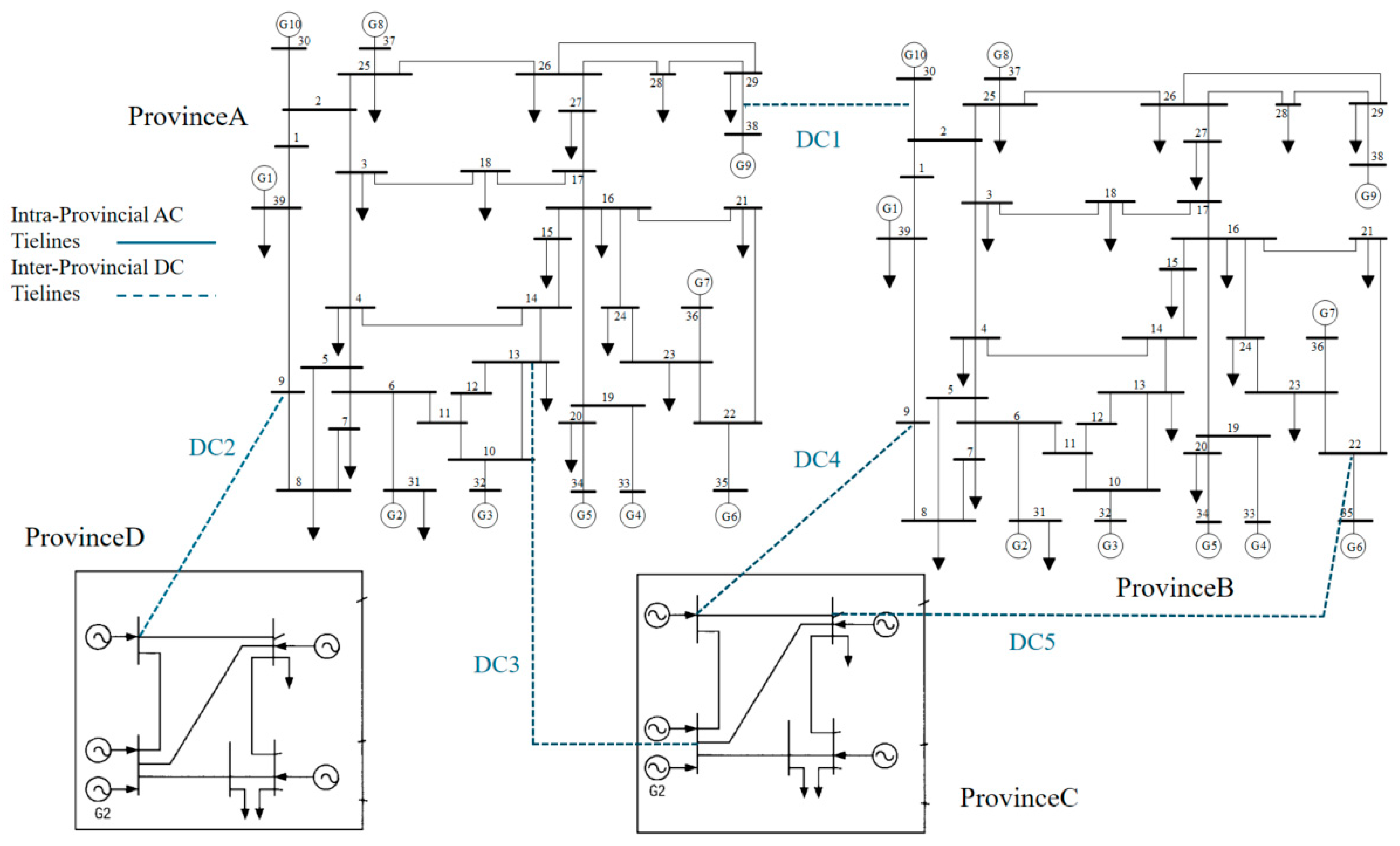
The test case is validated using a multi-area interconnected power system composed of four provincial grids (Province A, Province B, Province C, and Province D). Province A is connected to Province B, Province C, and Province D through three inter-provincial DC tie lines (DC1, DC2, and DC3), respectively. In addition, Province B is connected to Province C via two inter-provincial DC tie lines (DC4 and DC5). The overall interconnection architecture of the system is illustrated in Figure 1.

Regarding the internal network structures, the topology of Province A and Province B are based on the IEEE 39-bus test system, whereas Province C and Province D adopt the IEEE 5-bus test system topology. The entire multi-area system contains 88 buses in total. Based on the aforementioned regional network topology, four test cases are designed in this paper to validate the effectiveness of the models proposed in Section 2.1 and Section 2.2.

To ensure the validity of comparative analysis among different test cases, all cases adopt the same set of constraint components and operate under identical boundary conditions. To ensure practical relevance while maintaining strict data confidentiality regarding the actual grid, the operational dataset applied to this 88-bus framework is derived from the actual regional spot market data in the Southern Region of China. Highly realistic parameters—including load profiles, generator cost curves, physical unit limits, and tie-line scheduling boundaries—were meticulously mapped onto this standard test topology. Furthermore, rather than relying on theoretical academic computations, the Power Transfer Distribution Factor (PTDF) matrices utilized in this study are pre-processed, real-world shift factor matrices directly exported from the technical support system developed by NR Electric Group Corporation (Nanjing, China). The monitored section limits employed in the model represent the base-case (N-0) flow gate boundaries provided by the regional dispatch center, which inherently incorporate conservative N-1 security margins without requiring explicit endogenous contingency calculations. Computationally, the proposed topology-constrained flexibility assessment is formulated as a continuous Linear Programming (LP) problem (focusing on the real-time economic dispatch phase without binary unit commitment variables) and is solved using CPLEX 1280 solver.

Based on the aforementioned regional network topology and data configurations, six test cases are designed in this chapter to validate the effectiveness of the models proposed in Section 2.1 and Section 2.2. To ensure the validity of comparative analysis among different test cases, all cases adopt the same set of constraint components and operate under identical boundary conditions.

3.1. Comparative Case Study on Upward Flexibility Assessment

3.1.1. Description of Case Study

To systematically demonstrate the proposed multi-scenario assessment framework and thoroughly explore the grid’s physical boundaries under varying spatial stress conditions, four distinct load increment distribution patterns are established for comparison:

Scenario 1: This test case aims to investigate the maximum adjustable generation-side capability of the system under the most ideal spatial distribution of loads, which represents the theoretical upper bound of the system’s supply adequacy capability.

To establish a baseline scenario, this study adopts the computational model formulated in Section 2.2 (Equations (9) and (10)), which deliberately neglects the spatial distribution characteristics of loads. The fundamental premise of this RSCED-based benchmark is to concentrate all incremental loads entirely at the system’s slack bus. Consequently, the Power Transfer Distribution Factor (PTDF) for these increments equates to zero. This mathematical relaxation effectively eliminates the network congestion constraints typically triggered by spatially distributed loads, enabling the evaluation of the system’s absolute theoretical generation margin. Consequently, during the optimization process, the system temporarily ignores potential power flow limit violations on critical intra-provincial transmission corridors or inter-provincial DC tie lines that may arise from localized load surges.

The core computational logic of this test case is as follows: given the real-time operational boundaries, including generator output limits and scheduled power exchanges across inter-provincial and inter-regional tie lines, the model maximizes the total system load increment using a Regional Security-Constrained Economic Dispatch (RSCED) framework, with the overall system power and energy balance as well as the physical generation limits serving as the primary constraints.

Scenario 2: Uniform Distribution of Load Increments. In this scenario, load increments are distributed uniformly across all load nodes across the network. This acts as a standard reference condition to evaluate how general, system-wide average demand growth interacts with prevailing network transmission limits.

Scenario 3: Zonal Increments based on Province-Level Distribution. This scenario simulates a localized, extreme demand surge occurring exclusively within a specific load-center province such as driven by regional extreme weather events like heatwaves in a receiving-end province such as Guangdong). It aims to evaluate the cross-provincial power transfer capabilities and the specific flexibility deliverability when a single region experiences sudden load growth. The spatial distribution vector is parameterized such that the load participation factors are non-zero only for buses located within the target province. The increments within this zone are distributed proportionally to their baseline loads, while the load increment participation factors for all other provinces are strictly set to zero.

Scenario 4: Increments Concentrated at Heavily Loaded Nodes based on Worst-Case Robust Patterns. This scenario is designed as a severe operational stress test, serving as the worst-case scenario to address spatial load uncertainties. It evaluates the ultimate system flexibility when demand growth disproportionately occurs at the grid’s most congested and stressed load centers, which are typically the most vulnerable points for triggering the “capacity restriction effect.” The spatial distribution vector is strategically manipulated so that load increments are exclusively directed to a subset of nodes characterized by the highest initial baseline loads or nodes located downstream of critical flowgates). From a mathematical optimization perspective, this localized stress pattern represents the most adverse realization within a spatial distribution uncertainty polytope. By concentrating the increments at the most critical vertices of this distribution polytope, the model explicitly maximizes the congestion impact on limiting flowgates. This specifically pushes the local binding constraints to their absolute limits, allowing us to compute the minimum deliverable flexibility under uncertain spatial distributions. Consequently, this scenario successfully provides system operators with a robust lower bound of available capacity, guaranteeing that the assessed flexibility remains physically deliverable even under the most extreme and adverse demand growth trajectories.

3.1.2. Comparative Analysis of Upward Flexibility Case Study Results

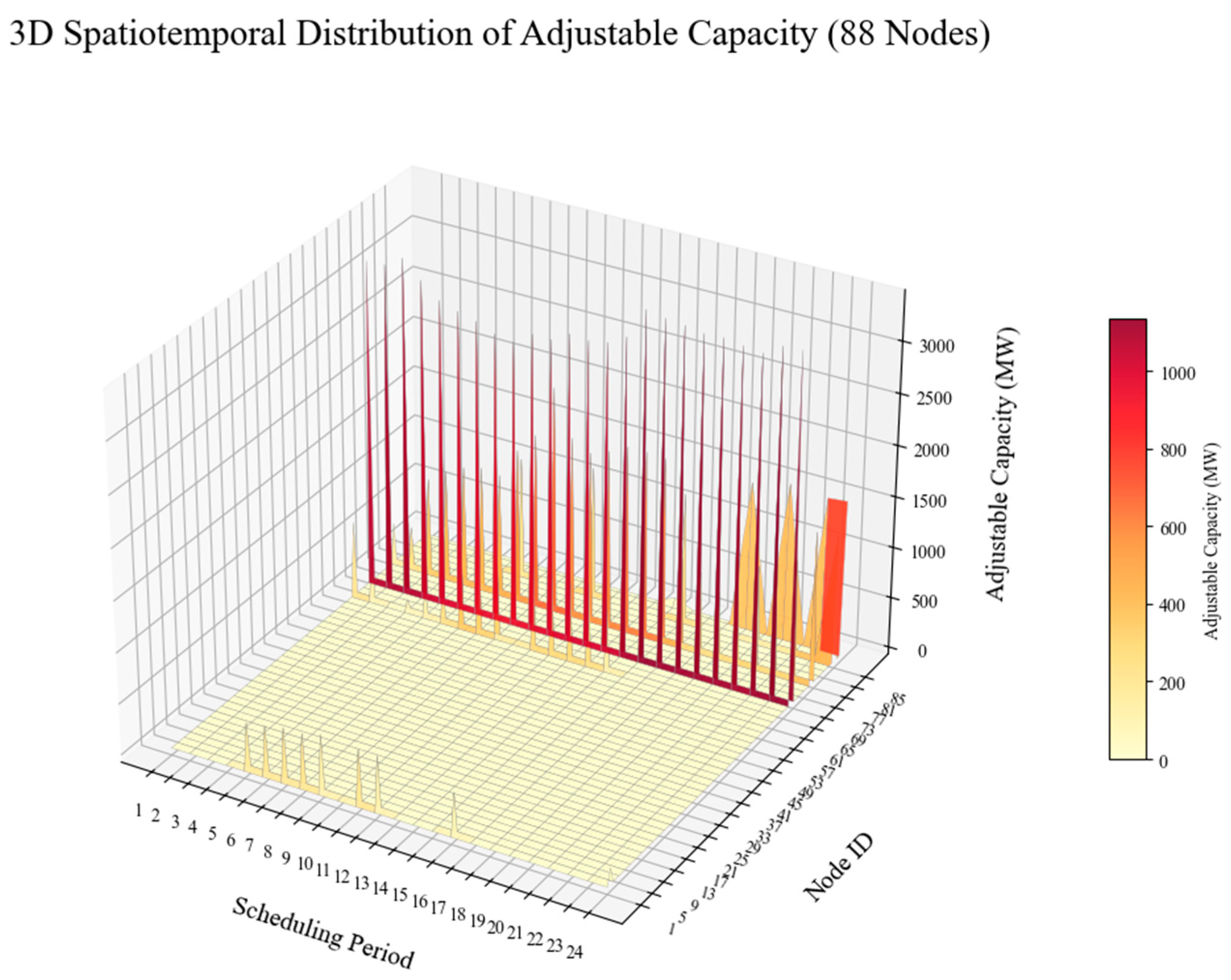
Figure 2 provides a 3D spatiotemporal surface plot depicting the evolution of the maximum adjustable capacity for the 88 nodes across all 24 scheduling periods. This visual intuitively integrates the drastic fluctuation characteristics in both temporal and spatial dimensions. Spatially, the towering “peaks” in the figure exclusively correspond to the system slack buses, which are mathematically configured to absorb the entirety of the load increments. Conversely, the expansive flat “plains” represent the non-slack nodes, whose adjustable capacities are rigidly constrained to zero. This distinct visual dichotomy perfectly illustrates the mathematical premise of the baseline model, where the spatial distribution of loads is entirely decoupled from the network topology. Temporally, even the high-capacity nodes that consistently maintain a dominant supporting role exhibit a noticeable “collapse” in their absolute capacity values (Z-axis height) during the evening peak periods (Periods 18–22). This 3D panoramic view not only corroborates the temporal scarcity of the overall system reserves but also confirms the topological rarity and high concentration of premium reserve resources. The unattenuated panoramic landscape of raw capacity under the baseline model establishes a visual and physical foundation for subsequently introducing improved models to quantitatively assess the capacity degradation effects caused by network security constraints.

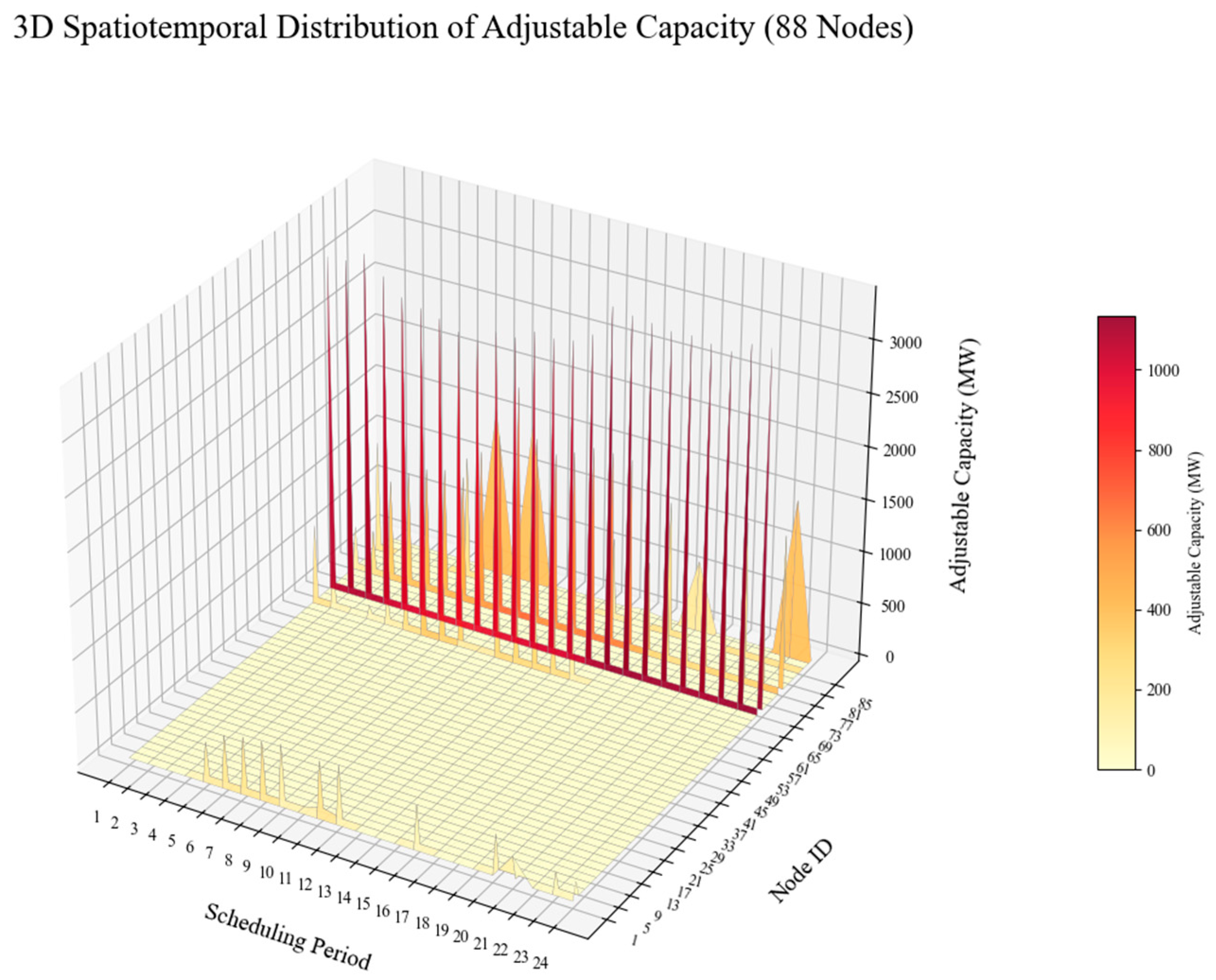
Figure 3 illustrates the 3D spatiotemporal evolution characteristics of the system’s adjustable reserve capacity under Improved Model I (the Uniform Distribution Strategy). Observing from the spatial dimension, the capacity increments of all participating active nodes remain absolutely identical within any single scheduling period, forming a strictly flat cross-section in the 3D space. This smooth surface feature visually verifies the effectiveness and high-precision solving capability of the strong-coupling equality constraints such as strict identical increments across nodes implemented in the underlying Security-Constrained Economic Dispatch (SCED) model.

From the temporal dimension, the adjustable capacity exhibits a significant alternating “peak-and-valley” pattern, which profoundly reveals the time-varying characteristics of the power grid’s physical operational boundaries. During off-peak hours, when the baseline load is low and transmission margins are abundant, all nodes can simultaneously achieve large load increments, forming the “peaks” on the surface. Conversely, during peak load periods, critical transmission corridors easily reach their thermal limits due to heavy baseline power flows. In this scenario, the strict uniform distribution mechanism triggers a pronounced “short-board effect” (wooden barrel effect): the increment potential of the entire network is forced to be constrained by a few of the most congested lines. Consequently, the capacities of all nodes decay synchronously and substantially, creating distinct “valleys” on the surface. This distribution graph clearly indicates that adopting a “one-size-fits-all” uniform response strategy—which ignores the spatial topological differences of the power grid—will severely restrict the total reserve potential of the system.

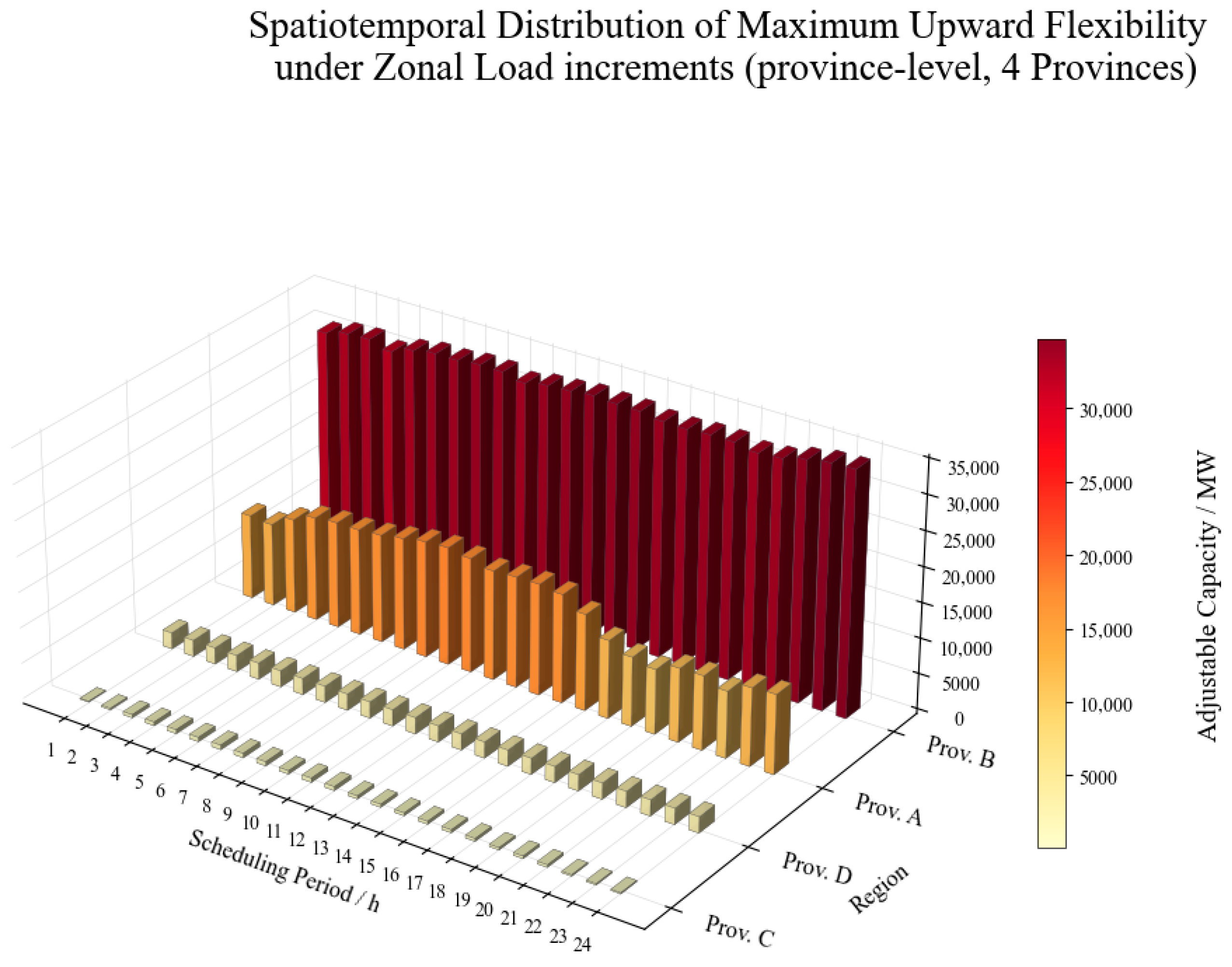
Figure 4 illustrates the quantitative spatiotemporal distribution of the maximum deliverable upward flexibility under the province-level zonal load increment scenario. The data reveals extreme spatial disparity and temporal volatility in actual deliverable capacity. Across the entire 24 h scheduling horizon, Province B maintains a consistently high upward flexibility margin, remaining stable at approximately 30,000 MW to 32,000 MW. In sharp contrast, Province A exhibits a distinct time-varying congestion bottleneck; its deliverable capacity sustains between 15,000 MW and 18,000 MW from period 1 to 15, but experiences a severe and continuous decline starting from period 16, ultimately dropping to below 10,000 MW during the late-peak hours. Furthermore, the deliverable upward capacities for Province C and Province D are strictly bottlenecked to near 0 MW throughout all 24 periods. This quantitative spatiotemporal contrast—where over 30,000 MW of flexibility remains accessible in Province B while Provinces C and D are continuously restricted to 0 MW—explicitly captures the physical magnitude of the capacity restriction effect, demonstrating that substantial theoretical reserves are structurally blocked by cross-provincial transmission limits.

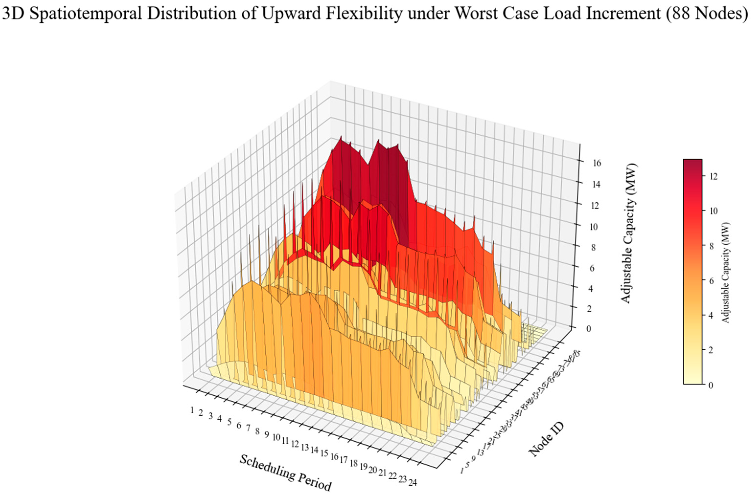
Figure 5 illustrates the quantitative 3D spatiotemporal distribution of the maximum deliverable upward flexibility across 88 nodes under the worst-case load increment scenario. In stark contrast to the preceding scenarios where the system-level deliverable capacities were consistently measured in tens of thousands of megawatts—such as the 30,000 MW margin previously observed in the province-level assessment—the deliverable capacity under this robust stress pattern collapses by several orders of magnitude. The vertical axis data explicitly demonstrates that the absolute maximum upward flexibility across the entire 88-node network peaks at merely 16 MW during the mid-scheduling periods (approximately periods 10 to 18). Furthermore, the vast majority of spatial nodes are strictly constrained to single-digit capacities, generally restricted to below 8 MW, and this minimal margin further plummets to near 0 MW across nearly all nodes during the early and late scheduling hours (periods 1 to 6 and 21 to 24). This dramatic numerical contraction from the 30,000-MW scale to the single-digit MW scale quantitatively maps the extreme lower bound of the capacity restriction effect, mathematically proving that when load increments are exclusively concentrated at the most critical downstream nodes, the resulting localized flowgate congestion completely strands the network-wide theoretical generation reserves, reducing the actual system deliverability to almost zero.

3.2. Comparative Case Study on Downward Flexibility Assessment

3.2.1. Description of Case Study

The case study in this section follows the same comparative logic as that in Section 3.1.1, but shifts focus to downward regulation flexibility. Specifically, it quantifies and contrasts the system’s total downward flexibility capacity under two distinct operational assumptions: (i) an idealized, network-constraint-free scenario—evaluated using the RSCED-Based Flexibility Assessment Benchmark Model, which determines the theoretical upper bound of downward regulation capacity; (ii) a realistic, network-constrained scenario—assessed via the Network-Constrained Flexibility Assessment Model, wherein load is uniformly distributed across the network to isolate the impact of transmission limits on downward flexibility deployment; (iii) a localized province-level increment scenario—wherein demand variations are exclusively confined to a specific target province, aimed at evaluating cross-provincial power transfer capabilities and downward flexibility deliverability under regional extreme events; (iv) a worst-case robust pattern scenario—designed as a severe operational stress test where load increments are strategically concentrated at heavily loaded nodes to maximize congestion impact, thereby determining the absolute lower bound of the system’s deliverable downward flexibility.

3.2.2. Comparative Analysis of Downward Flexibility Case Study Results

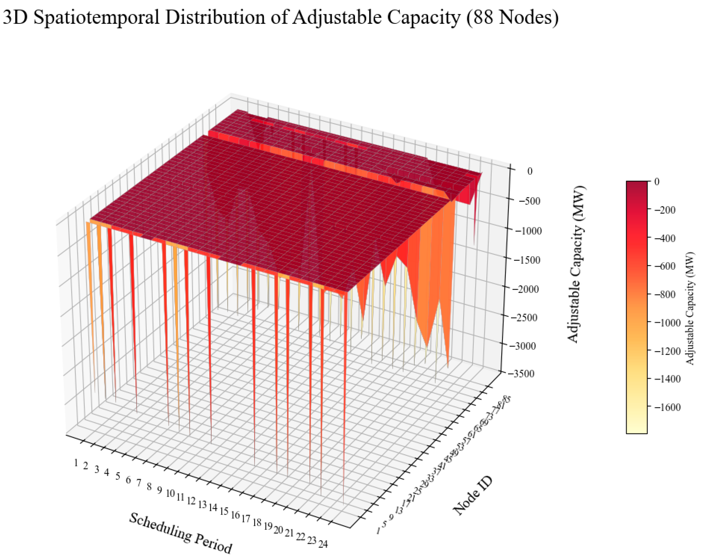
Figure 6 utilizes a 3D spatiotemporal surface plot to panoramically portray the entire evolution of the minimum adjustable capacity across 88 nodes and 24 periods. The expansive dark-colored (red) “plains” in the figure correspond to the set of nodes with zero downward capacity, further highlighting the deep scarcity dilemma of peak-shaving resources faced by the power grid across a wide spatiotemporal scope. In contrast, the light yellow “canyons” or “abysses” extending in the negative direction precisely pinpoint a minority of premium nodes with deep peak-shaving potential. Observed from the temporal dimension, the depth of these deep valleys exhibits regular undulations and contractions alongside the scheduling periods; analyzed from the spatial dimension, the discrete distribution of premium downward resources across the physical topology is abundantly clear. This panoramic view confirms that even under the ideal baseline model, which temporarily disregards network congestion triggered by the deterioration of wide-area load distribution, the system’s fundamental bottom-line downward capacity remains extremely concentrated and scarce. This provides an indispensable baseline view for the subsequent introduction of quantitative risk assessments that incorporate nodal distribution characteristics.

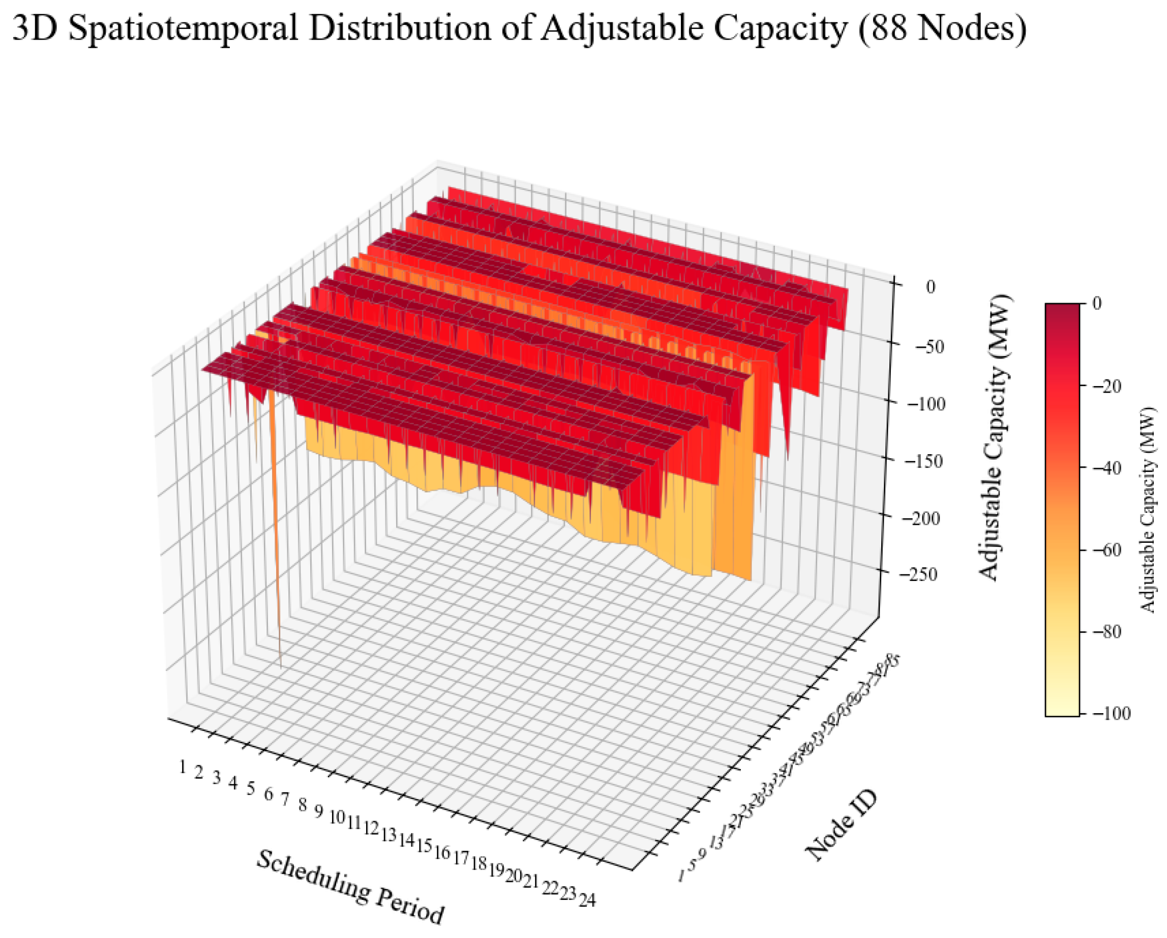
Figure 7 utilizes a 3D spatiotemporal surface plot to panoramically display the evolution of the nodal downward capacity across the 88 target nodes and 24 scheduling periods under Improved Model I. Distinct from the abundant negative regulatory space observed in the baseline model, this figure presents a stark “severe compression” characteristic across the spatiotemporal domain. During the early morning load valley periods, the system retains a certain degree of downward regulation margin, manifested visually as several distinct localized “trenches” extending into the deeper negative domain. However, as the scheduling progresses into the daytime and evening peak periods (Periods 7–24), the downward capacity across the vast majority of nodes experiences a precipitous contraction. The spatiotemporal surface transitions into a highly compressed, shallow plateau hovering critically close to the 0 MW axis (predominantly restricted within a narrow band of 0 to −20 MW). This 3D panoramic view visually corroborates that, under the stringent constraint of wide-area uniform load reduction, the downward regulation actions rapidly exhaust the transmission margins of critical network flowgates. Consequently, the physical peak-shaving potential of the generating units suffers from a widespread network-induced “lockdown,” proving to be far more scarce than anticipated by traditional dispatch experience.

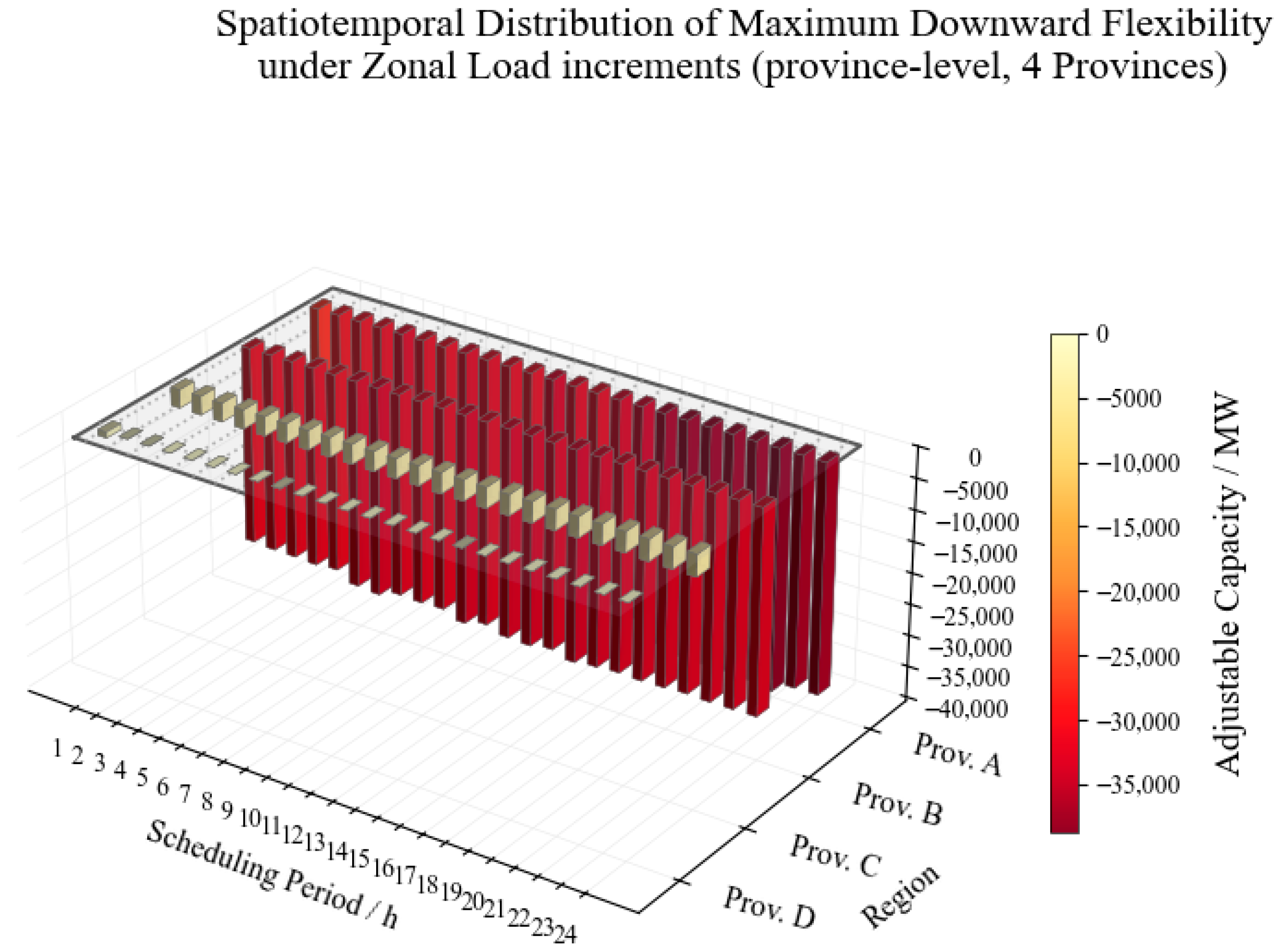
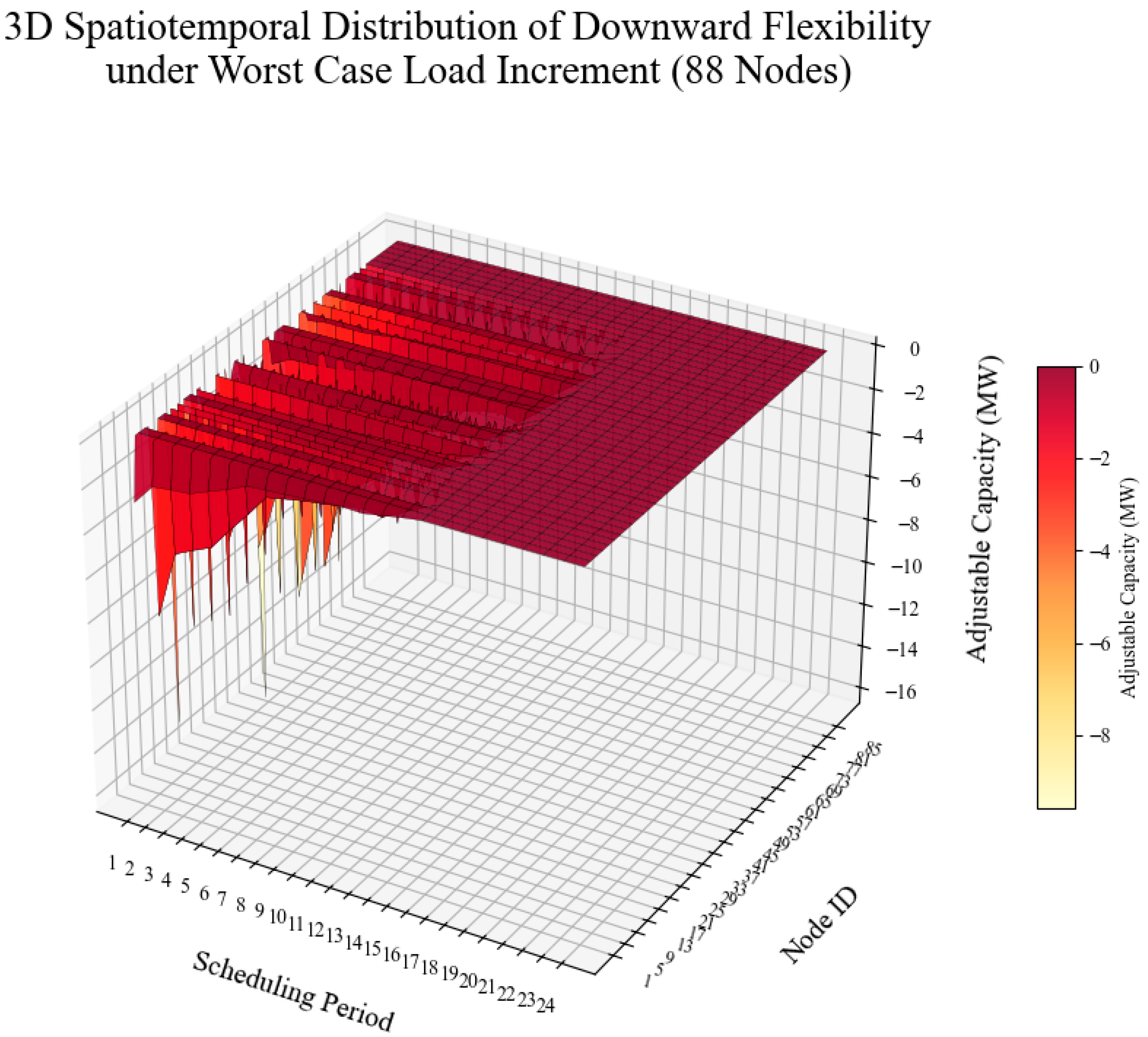
Figure 8 and Figure 9 presents a comparative spatiotemporal analysis of the maximum downward flexibility under two distinct load variation paradigms: a localized provincial load increment and a worst-case robust pattern concentrated at heavily loaded nodes. In Scenario 3, the load increment is directed to a specific province, with the increment participation factors for other provinces set to zero. Under this spatial distribution, the system maintains a significant downward regulation margin. As illustrated in the left panel, the deliverable downward capacities reach the magnitude of ${10}^4$ mw, extending to approximately −35,000 MW. This indicates that when load variations are confined to a single target province, the cross-provincial transmission capacity can support the transfer of downward flexibility from other regions to maintain system balance.

In Scenario 4, load increments are concentrated at the grid’s heavily loaded nodes, representing the worst-case boundary within the spatial distribution uncertainty polytope. Under this pattern, the capacity restriction effect becomes evident. As depicted in the right panel, the scale of deliverable capacity is restricted to a narrow range of 0 to −16 MW. Spatiotemporally, the downward flexibility for the 88 nodes across the 24 h horizon is primarily constrained at 0 MW, forming a flat zero-value surface. This numerical comparison demonstrates that concentrating demand growth at critical load centers maximizes the congestion impact on limiting flowgates, causing local binding constraints to reach their limits and thereby reducing the minimum deliverable flexibility of the network to near zero.

3.3. Comparative Discussion of Multi Cases Assessment

3.3.1. Comparative Analysis of Four Case Study Results for Upward Flexibility

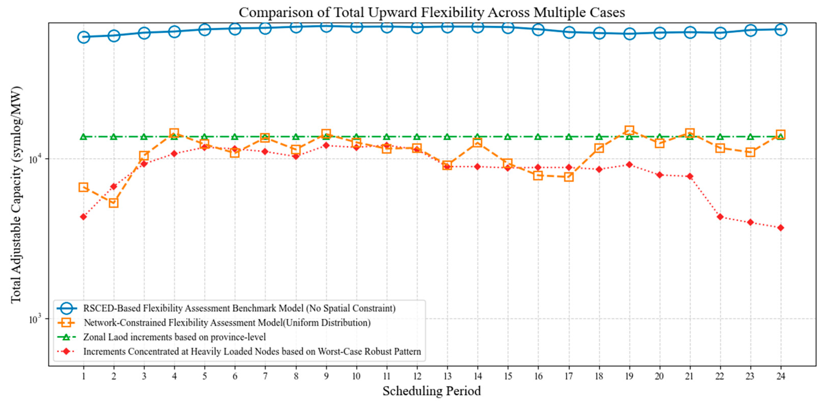
Figure 10 illustrates the comparative temporal evolution of the system’s total upward flexibility across a 24 scheduling horizon under an unconstrained benchmark model and network-constrained models with different spatial distribution assumptions.

This significant reduction in total deliverable flexibility is mathematically driven by the binding transmission constraints at specific flowgates, which strictly limit further load increments. The global upward boundary is rigidly bottlenecked by the earliest occurrence of localized transmission congestion, thereby rendering massive generation reserves located in uncongested areas undeliverable. Furthermore, unlike the smooth baseline, the network-constrained capacities exhibit highly jagged, non-linear oscillations that directly map the sensitivity of the feasible region to the power flow. Throughout the scheduling cycle, the critical binding constraints frequently migrate across the spatial grid topology, driving the high-frequency volatility in the total capacity boundary. Among the constrained scenarios, the zonal province-level increment model partially smooths out intra-zonal bottlenecks, whereas the worst-case robust pattern establishes the absolute lower bound of the system’s flexibility.

The stark divergence between the unconstrained and constrained curves quantitatively validates that neglecting network topology leads to a profound, structurally flawed overestimation of system adequacy. It proves that real-time upward flexibility is not a simple scalar aggregation of generation margins, but a complex state variable strictly bounded by the dynamic spatial coupling of load distribution and network congestion.

3.3.2. Comparative Analysis of Four Case Study Results for Downward Flexibility

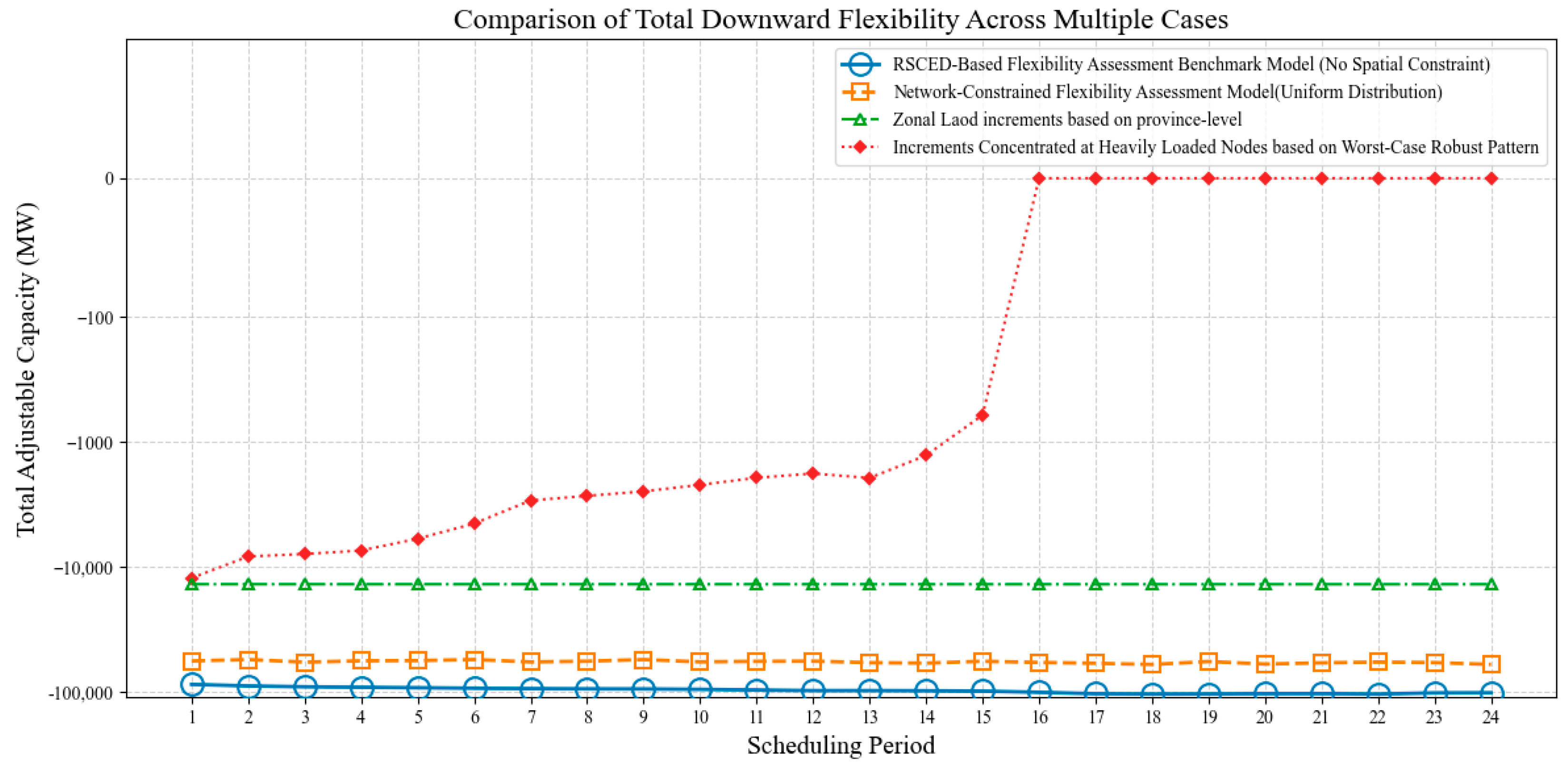
Figure 11 illustrates the time-interval aggregated downward flexibility under the same four assessment paradigms. Consistent with the upward scenario, the unconstrained benchmark (blue circles) establishes the maximum theoretical boundary. The integration of network constraints significantly reduces the deliverable downward capacity across all scenarios.

However, the relative impact of spatial distribution assumptions diverges fundamentally from the upward assessment. The bus-level uniform distribution model (orange squares) preserves a substantial portion of the downward margin. In contrast, the zonal province-level model (green triangles) imposes a much stricter limitation, maintaining a rigidly constrained capacity near −10,000 MW. This indicates that downward regulation capability is predominantly restricted by inter-provincial tie-line bottlenecks rather than intra-zonal allocations.

Furthermore, the worst-case robust pattern (red diamonds) identifies the absolute minimum downward flexibility. Under this paradigm, the deliverable capacity sharply deteriorates after period 14 and is completely exhausted (0 MW) between periods 16 and 24. This complete depletion demonstrates that localized network congestion, when aligned with adverse spatial load variations, can entirely eliminate the system’s downward regulation margin.

Collectively, these results reinforce the conclusion that flexibility is a strictly topology-dependent state variable. Neglecting spatial constraints or adopting inappropriate spatial assumptions leads to severe overestimation of system adequacy in both upward and downward directions.

3.3.3. Analysis of Binding Constraints and the Capacity Restriction Mechanism

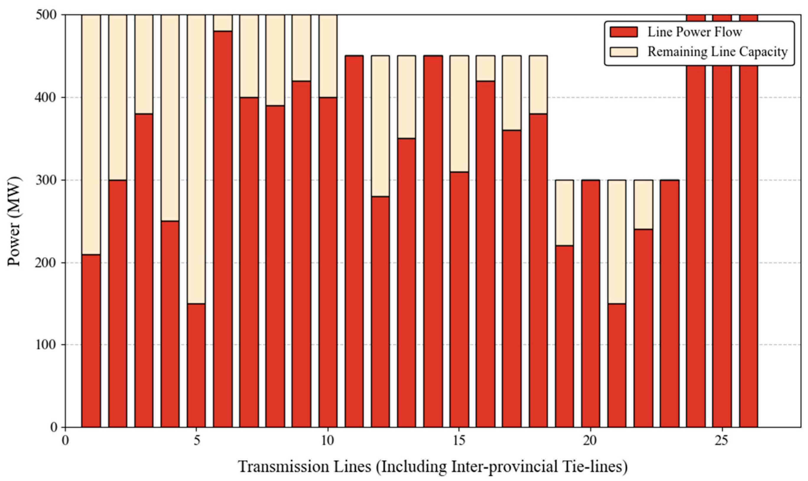
This subsection investigates the physical mechanism driving the “capacity restriction effect” by analyzing the activation of key transmission security constraints. Taking the upward flexibility assessment in Scenario 3 (localized provincial load increment) as an illustrative example, Figure 12 visually quantifies the capacity restriction mechanism by presenting the active power flows and remaining capacities of the transmission branches.

As explicitly illustrated, several critical transmission corridors—specifically lines 11, 15, 23, 24, 25, and 26—have completely exhausted their available transfer margins. Their active power flows strictly hit the thermal limits, reducing the remaining capacity to zero. From an optimization perspective within the RSCED framework, these specific branches transition into active binding constraints. Once these limiting interfaces are dynamically activated, the interconnected grid becomes physically bottlenecked. Governed by the network’s PTDF sensitivity matrix, any further deployment of downward flexibility from resources located upstream of these congested corridors is strictly prohibited to prevent thermal overloads. This analytical evidence directly demonstrates how localized transmission bottlenecks mathematically and physically trigger the system-wide “capacity restriction effect.”

3.3.4. Data Boundaries and Solver Description

To ensure the fairness and validity of the multi-case comparative assessment in this study, strictly consistent initial system boundary conditions are applied across all test scenarios. These common boundary parameters specifically encompass: the operational cost data of generating units, the sensitivity matrices characterizing the physical network topology, the predefined scheduling targets for inter-provincial priority trading plans, and the overall renewable energy penetration ratio of the system. By strictly controlling these underlying variables, the case study results effectively eliminate the interference of extraneous factors, thereby intuitively and objectively depicting the direct impact of distinct constraint conditions on the global flexibility margin.

It should be specifically noted that the sensitivity matrices, detailed unit parameters, and actual load profiles utilized in this study are derived from the real-world operational data of the China Southern Power Grid (CSG). Due to data confidentiality and sensitivity restrictions, the complete underlying parameter details cannot be publicly disclosed; however, the unit composition and renewable energy data of the system have been explicitly presented.

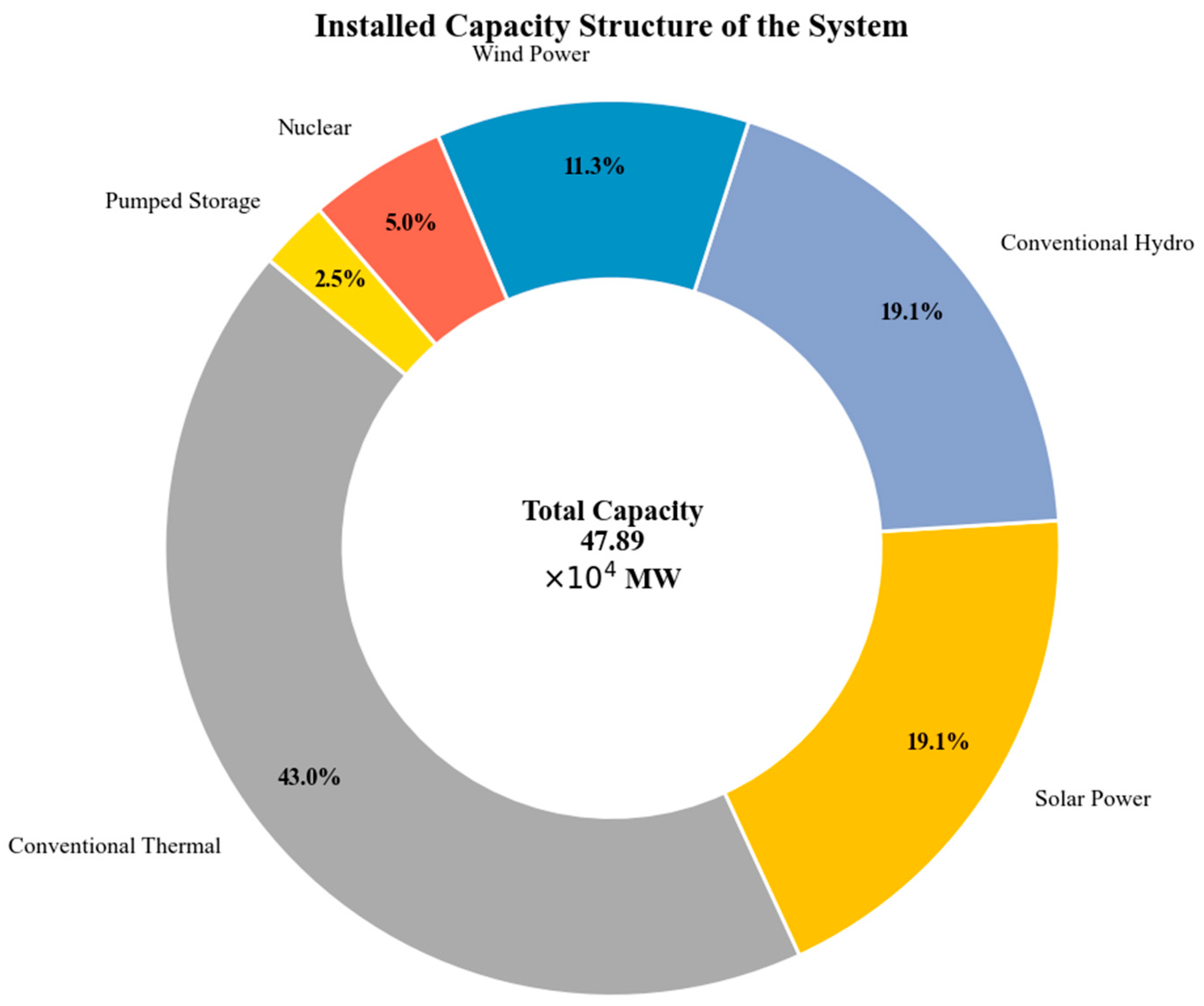
Regarding renewable energy, our assessment establishes a representative static baseline under a high-penetration scenario, rather than generating dynamic stochastic variability profiles. As detailed in the revised case description, we explicitly illustrated the substantial installed capacity share of renewable energy in the targeted system. This high-penetration condition serves as the fundamental initial boundary state for evaluating the system’s baseline flexibility. Figure 13 illustrates the breakdown of installed capacity for various types of renewable energy units across the entire network. As the data clearly indicates, renewable energy accounts for 57% of the total installed capacity.

All above case study is formulated as a continuous Linear Programming (LP) problem. The simulations were conducted on a high-performance personal workstation utilizing a multi-core CPU with 16 parallel threads. The model was implemented in a C++ programming environment and solved using a commercial mathematical programming solver. Because it is an LP formulation, the model deterministically converges to the global optimal solution with a 0.00% optimality gap. The total computational runtime for simulating the entire 24-period day-ahead horizon is approximately 140 s. This high computational efficiency fully satisfies the strict time constraints required for practical market clearing operations.

4. Conclusions

In this paper, a multi-scenario flexibility capability assessment model formulated upon RSCED framework was proposed to accurately quantify the deliverable reserve of adjustable resources in regional electricity spot markets. Moving beyond traditional capacity-accumulation methods, this study systematically proved that the actual dispatchable margin of a wide-area interconnected grid is fundamentally constrained by network topological bottlenecks rather than the physical limits of individual generators. The observed “capacity restriction effect” and the high-frequency temporal oscillation of available reserves highlight a strong spatiotemporal coupling between power flows and spatial load distributions. Specifically, the compact analysis of binding constraints reveals that during peak and sub-peak scheduling periods, critical transmission corridors—primarily the cross-provincial DC tie-lines 1,4,3—frequently hit their thermal limits, acting as the exact physical bottlenecks that trigger the restriction mechanism. Furthermore, the comparative evaluations demonstrate that while cross-provincial power transfer capabilities can partially sustain deliverable margins under localized provincial demand surges, the system remains acutely vulnerable to worst-case spatial distributions. As evidenced by the robust stress test, concentrating load increments at critical heavily loaded nodes drives local binding constraints to their absolute physical limits, thereby establishing an absolute lower bound that can completely eliminate the system’s deliverable flexibility. These findings demonstrate the inherent dynamic vulnerability of the system and render static reserve methodologies obsolete for modern grid operations. Consequently, the pervasive “short-board effect” identified in the spatial transmission network necessitates a paradigm shift in real-time dispatch and market clearing mechanisms. From a practical and policy perspective, this research provides a robust theoretical foundation for transitioning toward topology-aware, dynamic reserve monitoring in spot markets. Furthermore, it underscores the profound strategic and economic value of deploying targeted flexible resources—such as distributed energy storage or dynamic line rating technologies—at critical congestion nodes to effectively unlock trapped system-wide capacities.

Nevertheless, it should be noted that the numerical experiments are conducted on a standardized test system and rely on simplified load distribution assumptions, which may limit the direct quantitative generalizability of the results. These simplifications are adopted to isolate the underlying mechanism of topology-induced flexibility restriction and do not affect the general validity of the proposed framework.

Future research will focus on the coordinated optimal scheduling of these localized flexible resources to actively alleviate the identified spatiotemporal constraints.

References

1. Lin, Y.S.; Lu, Z.X.; Qiao, Y. Temporal-Probabilistic Power and Energy Balance Theory Based on a Feasible Region Model of Adjustable Resources. Autom. Electr. Power Syst. 2025, 49, 61–72. [Google Scholar]
2. Zhang, R. Research on Assessment of Regulation Participation Capacity and Unbalanced Dispatch in New Urban Power Grids. Ph.D. Thesis, Harbin Institute of Technology, Harbin, China, 2024. [Google Scholar] [CrossRef]
3. Chen, Z. Research on Reserve Optimization and Distributed Dispatch of Power Systems with High-Proportion Wind Power. Ph.D. Thesis, Zhejiang University, Hangzhou, China, 2021. [Google Scholar] [CrossRef]
4. Song, Z.; Zhang, L.; Zhang, Z. Value Evaluation of New Dispatchable Resources in Power Systems. In Proceedings of the 8th International Conference on Electrical Engineering and Green Energy (CEEGE), Yangzhou, China, 4–6 July 2025; pp. 309–314. [Google Scholar]
5. Zhang, Y.Z. Adjustable Value Assessment and Aggregation Analysis of Distribution Network Loads. Master’s Thesis, Nanjing University of Posts and Telecommunications, Nanjing, China, 2022. [Google Scholar] [CrossRef]
6. He, S.Q.; Jiang, H.; Wu, C.F.; An, R.J. Analysis of Regional Adjustable Capacity and Collaborative Optimization Based on an Aggregation Model of Air-Conditioner Clusters. Power Big Data 2025, 28, 9–18. [Google Scholar] [CrossRef]
7. Wang, Y.; Zhu, L.; Fang, Y.; Zhou, J.; Liu, C. Power System Day-Ahead and Intra-Day Optimal Scheduling Considering Flexible Coordination of Steel Production and Energy Storage. Energies 2026, 19, 1209. [Google Scholar] [CrossRef] [Scilit]
8. Tai, X.; Li, Z.H.; Chen, Z.Y.; Zhu, Q.; Wang, Q. Assessment of the Maximum Power Supply Capacity of Distribution Networks with N-1 Compliance Rate Constraints. Shandong Electr. Power Technol. 2024, 51, 65–73. [Google Scholar] [CrossRef]
9. Kong, X.Y.; Liu, C.; Chen, S.S.; Chen, Q.X.; Wang, Z.T. A Method for Assessing the Response Potential of Adjustable Resource Clusters at Multiple Time Nodes Considering Dynamic Processes. Autom. Electr. Power Syst. 2022, 46, 55–64. [Google Scholar]
10. Ajao, Q.; Sadeeq, L. A Rapidly Dispatchable Energy Strategy Utilizing Electric Vehicles with Energy Storage Systems (EV-ESS) to Enhance Grid Redundancy. Smart Grids Sustain. Energy 2025, 10, 7. [Google Scholar] [CrossRef] [Scilit]
11. Wang, J.; Wen, J.F.; Zhang, F.Y. The Optimal Allocation of Dispatchable Resources Considering the Flexibility of Microgrid. J. Phys. Conf. Ser. 2020, 1678, 012041. [Google Scholar] [CrossRef] [Scilit]
12. Lv, W.Q.; Liu, Z.W.; Dong, X.X.; Zhu, J.T.; Yuan, Y. A Cluster Partitioning Method Considering the Adjustable Capacity and Response Speed of Flexible Resources. Power Eng. Technol. 2024, 43, 37–47. [Google Scholar]
13. Zhou, Y.; Li, Y.C.; Fu, Y.S.; Qin, K.P.; Zhu, W.; Fan, D.Q. Research on Optimal Unit Commitment Decision-Making with the Participation of Power Grid Flexible Reserves. J. Harbin Univ. Sci. Technol. 2023, 28, 56–66. [Google Scholar] [CrossRef]
14. Wu, D.; Zheng, J.; Li, Y.; Huang, J.; Xiao, S. A Study on the Optimization of Dispatch Mechanisms with the Participation of Flexible Resources in Power Grid Regulation. In Proceedings of the 4th International Conference on Smart Grids and Energy Systems (SGES), Guiyang, China, 11–13 July 2025; pp. 33–37. [Google Scholar]
15. Zhong, L.; Yang, M.; Liu, S.; Liu, T.; Bian, X.; Tong, L. Bi-Level Coordinated Planning of Port Multi-Energy Systems Considering Source-Load Uncertainty Based on WGAN-GP and SBOA. Energies 2026, 19, 1160. [Google Scholar] [CrossRef] [Scilit]
16. Zheng, T.; Litvinov, E. Contingency-Based Zonal Reserve Modeling and Pricing in a Co-Optimized Energy and Reserve Market. IEEE Trans. Power Syst. 2008, 23, 277–286. [Google Scholar] [CrossRef] [Scilit]
17. Wang, F.; Chen, Y. Market Implications of Short-Term Reserve Deliverability Enhancement. IEEE Trans. Power Syst. 2021, 36, 1504–1514. [Google Scholar] [CrossRef] [Scilit]
18. Ye, H.; Ge, Y.; Shahidehpour, M.; Li, Z. Uncertainty Marginal Price, Transmission Reserve, and Day-Ahead Market Clearing with Robust Unit Commitment. IEEE Trans. Power Syst. 2017, 32, 1782–1795. [Google Scholar] [CrossRef] [Scilit]
19. Leite da Silva, A.M.; Costa Castro, J.F.; González-Fernández, R.A. Spinning Reserve Assessment Under Transmission Constraints Based on Cross-Entropy Method. IEEE Trans. Power Syst. 2016, 31, 1624–1632. [Google Scholar] [CrossRef] [Scilit]
20. Chen, W.; Park, S.; Tanneau, M.; Van Hentenryck, P. Learning optimization proxies for large-scale Security-Constrained Economic Dispatch. Electr. Power Syst. Res. 2022, 213, 108566. [Google Scholar] [CrossRef] [Scilit]
21. Gbadega, P.A.; Sun, Y. Synergistic Integration of Renewable Energy and HVDC Technology for Enhanced Multi-objective Economic Emission Dispatch Using the Salp Swarm Algorithm. In Neural Computing for Advanced Applications; Zhang, H., Li, X., Hao, T., Meng, W., Wu, Z., He, Q., Eds.; NCAA 2024. Communications in Computer and Information Science; Springer: Singapore, 2025; Volume 2182. [Google Scholar] [CrossRef] [Scilit]
22. Navid, N.; Rosenwald, G. Market solutions for managing ramp flexibility with high penetration of renewable resource. IEEE Trans. Power Syst. 2012, 27, 284–292. [Google Scholar] [CrossRef] [Scilit]
Figure 1. Topology of the test system.
Energies 19 02501 g001
Figure 2. Spatiotemporal distribution of maximum adjustable capacity for case3.1 based on ideal spatial distribution.
Energies 19 02501 g002
Figure 3. Spatiotemporal distribution of maximum adjustable capacity for case3.1 based on uniform distribution.
Energies 19 02501 g003
Figure 4. Spatiotemporal distribution of maximum upward flexibility under zonal load increments (province-level) for case3.1.
Energies 19 02501 g004
Figure 5. Spatiotemporal distribution of maximum upward flexibility under worst case load increments for case3.1.
Energies 19 02501 g005
Figure 6. Spatiotemporal distribution of downward adjustable capacity for case3.2 based on uniform distribution.
Energies 19 02501 g006
Figure 7. Spatiotemporal distribution of downward adjustable capacity for case3.2.
Energies 19 02501 g007
Figure 8. Spatiotemporal distribution of downward adjustable capacity under zonal load increments for case3.2.
Energies 19 02501 g008
Figure 9. Spatiotemporal distribution of downward adjustable capacity under worst-case increments for case3.2.
Energies 19 02501 g009
Figure 10. Time-interval aggregated upward flexibility at the bus level for multicase comparisons for case3.1.
Energies 19 02501 g010
Figure 11. Time-interval aggregated adjustable capacity at the bus level for multicase comparisons for case3.2.
Energies 19 02501 g011
Figure 12. Schematic diagram of key line power flow and remaining transmission capacity.
Energies 19 02501 g012
Figure 13. Description of the boundary conditions of the units including the proportion of installed capacity of various new energy sources.
Energies 19 02501 g013
Disclaimer/Publisher’s Note: The statements, opinions and data contained in all publications are solely those of the individual author(s) and contributor(s) and not of MDPI and/or the editor(s). MDPI and/or the editor(s) disclaim responsibility for any injury to people or property resulting from any ideas, methods, instructions or products referred to in the content.