Risk-Aware Trading Signals for Smart Aggregators in Multi-Time-Scale Electricity Markets Using Regime-Switching and Tail-Risk Analysis

Abstract

With the rapid expansion of renewable energy and the formal operation of provincial electricity spot markets in China, smart aggregators that coordinate flexible loads, storage resources, demand-response portfolios, and distributed energy resources increasingly face imbalance-settlement risk across the day-ahead and real-time segments of the electricity spot market. Existing studies often focus on average prices or point forecasts, which may overlook regime persistence, negative-price clustering, and tail exposure in high-frequency price spreads. This paper develops a regime-switching and tail-risk signal framework to characterize and forecast day-ahead–real-time price spreads in the Shandong electricity spot market and to translate these forecasts into risk-aware trading signals for representative smart aggregators. Using 35,136 non-public observations at 15 min resolution provided by State Grid Shandong Electric Power Company for 2024, the spread is analyzed using descriptive statistics, Markov regime-switching models, quantile regression, out-of-sample forecasting, trading-signal backtesting, component ablation, and robustness checks. The spread, defined as real-time price minus day-ahead price, has a mean of −7.50 Chinese yuan per megawatt-hour (CNY/MWh), a median of −0.005 CNY/MWh, 5% and 95% quantiles of −196.84 and 137.65 CNY/MWh, and 1% and 99% quantiles of −372.68 and 338.04 CNY/MWh, respectively. A three-state Markov model identifies negative-deviation high-volatility, near-zero low-volatility, and positive-deviation regimes with multi-hour persistence. In the December out-of-sample test, the upper- and lower-tail quantile signals achieve recall rates of 0.872 and 0.841, respectively, and removing lagged spreads increases mean absolute error (MAE) from 24.015 to 54.278 CNY/MWh. The framework provides risk-warning signals rather than causal identification or realized-profit evaluation.

1. Introduction

The electricity spot market transmits marginal-cost, supply–demand, and scarcity signals in power systems with increasing shares of variable renewable energy. Wind and solar generation alter net-load profiles, ramping needs, and short-term forecast uncertainty, which can contribute to negative prices, spikes, and heavy-tailed volatility. Smart aggregators coordinate flexible loads, storage, demand response, distributed generation, and other controllable resources across the day-ahead and real-time segments of the electricity spot market; their imbalance-settlement exposure is therefore closely linked to deviations between day-ahead expectations and real-time outcomes. In the title of this article, “multi-time-scale electricity markets” refers to the linked day-ahead and real-time segments and the 15 min-to-hourly analytical resolutions within the Shandong electricity spot market; it does not denote multiple independent regional markets or unrelated market types. Shandong provides a policy-relevant case because its electricity spot market entered formal operation on 17 June 2024 [1], while renewable capacity exceeded 100 gigawatts (GW) [2].

In a two-settlement design, day-ahead prices are formed from forecast demand, expected renewable generation, unit conditions, bids, and anticipated operating boundaries, whereas real-time prices absorb realized imbalances and updated system conditions. Network and infrastructure constraints, interprovincial power flows, and reserve requirements can also materially affect next-day price formation and the subsequent spread [3,4]. For a smart aggregator, a positive real-time-minus-day-ahead spread may raise real-time procurement costs or reward flexible injection and demand reduction; a negative spread may create low-price adjustment opportunities while reducing the settlement value of previously scheduled supply. The spread is therefore used here as a market-facing risk signal, not as a direct measure of any single physical driver.

1.1. Background and Motivation

Prior research identifies two complementary channels through which renewable integration affects electricity prices. The merit-order effect can depress prices when low-marginal-cost wind and solar generation is abundant [5], while limited flexibility, operating constraints, and forecast deviations can intensify negative-price episodes and tail volatility [6,7,8,9]. These findings motivate distributional and state-dependent analysis: extreme observations should be treated as economically informative market outcomes rather than deleted as ordinary outliers.

The methodological implication is that a mean forecast alone cannot distinguish a brief 15 min deviation from a persistent risk regime. This study therefore focuses on the real-time-minus-day-ahead spread defined in Equation (1), asks whether its distribution switches among persistent states, and estimates its conditional lower and upper tails. This framing links high-frequency price behavior to the timing of exposure-control decisions without attributing observed spreads to unmeasured renewable, network, reserve, or bidding variables.

1.2. Literature Review and Research Gap

The first strand of the literature examines renewable energy, negative electricity prices, and electricity price formation. Hirth argues that the market value of variable renewable energy declines as penetration increases, with time-matching, spatial constraints, and forecast errors being important contributing factors [5]. Seel et al. further interpret negative prices as price outcomes jointly driven by high renewable output, low load, and insufficient system flexibility [6]. Using European balancing-market data, Brijs et al. find that negative prices exhibit clear statistical regularities and event clustering, and therefore should not be treated simply as outliers [9]. These studies imply that negative and extreme prices are informative market outcomes rather than noise to be removed before modeling.

The second strand focuses on price discovery and imbalance risk in day-ahead and real-time markets. Weron’s review highlights that electricity price forecasting differs from general commodity-price forecasting because electricity prices display high frequency, seasonality, spikes, mean reversion, and institutional dependence [10]. In two-settlement markets, day-ahead prices reflect participants’ expectations regarding next-day supply and demand, whereas real-time prices absorb actual operational deviations. Woo et al. link renewable-induced price changes to day-ahead–real-time price spreads in California, showing that the spread captures the deviation between market expectations and actual operation [7]. However, existing studies have mainly focused on mature European and U.S. markets, and high-frequency evidence on provincial spot markets in China, particularly after the formal operation of the Shandong market, remains relatively limited.

The third strand adopts a regime-switching perspective. Hamilton’s Markov regime-switching model provides a classic framework for characterizing nonlinear and nonstationary time series [11]. In electricity price studies, price spikes, negative prices, and normal fluctuations often do not arise from a single data-generating process, but instead reflect switching among different market regimes. The advantage of a regime-switching model is that it can estimate regime-specific means, volatilities, persistence probabilities, and transition matrices, thereby answering which regime the market is currently in and how long that regime may persist. For the Shandong day-ahead–real-time spread, this perspective is particularly important: if negative prices or extreme spreads are persistent, imbalance-risk management should focus not only on errors at individual time points, but also on regime transitions and continuous exposure.

The fourth strand characterizes price risk through the conditional distribution rather than the conditional mean. Quantile regression, introduced by Koenker and Bassett, estimates the effects of explanatory variables at different quantiles [12], and Koenker and Hallock further clarify its interpretive value in economic analysis [13]. In electricity price research, Maciejowska uses quantile regression to assess the impact of renewable energy on price levels and volatility, showing that renewable energy affects different parts of the price distribution differently [14]. Hagfors et al. model electricity price distributions in the United Kingdom using quantile regression, and show that the method is well suited to non-normality and tail behavior in electricity prices [15]. These studies provide the methodological foundation for the present paper: the average effect of the Shandong spread may be weak, whereas load, load change, day-ahead price, and intraday variables may exert stronger marginal effects at the 5%, 10%, 90%, or 95% quantiles [16].

Overall, the existing literature has separately documented the effects of renewable energy on price formation, the statistical significance of negative and extreme prices, the ability of regime-switching models to characterize nonlinear price processes, and the suitability of quantile regression for tail-risk analysis [17,18]. Some related studies on virtual power plants, demand response, and resource aggregators emphasize that aggregated flexible resources can participate in electricity markets and provide system flexibility [19,20,21]. Nevertheless, four gaps remain. First, empirical evidence on high-frequency day-ahead–real-time spreads in Chinese provincial spot markets, especially around the formal operation of the Shandong market, is still insufficient. Second, existing studies often discuss negative prices, price forecasting, or mean spreads separately, whereas negative prices, price spikes, and heavy-tailed deviations are less frequently integrated into a unified regime-switching and conditional-distribution framework. Third, many forecasting studies rely on random train–test splits or report only mean squared errors, which may overlook time series information leakage, component-level contribution, and extreme-event prediction performance. Fourth, aggregator trading studies often begin from an optimization or bidding model with assumed price forecasts, whereas fewer studies first examine whether high-frequency day-ahead–real-time spreads contain persistent regimes and tail-risk signals that can guide risk-aware trading before solving a full dispatch problem. This paper aims to provide additional evidence on these issues.

1.3. Research Questions and Hypotheses

This study addresses five method-centered questions. It examines whether the spread has asymmetric heavy tails and systematic temporal heterogeneity; whether economically interpretable and persistent regimes can be identified; whether load, load change, day-ahead price, intraday timing, and lagged spreads shift the lower and upper conditional quantiles differently; whether time-ordered out-of-sample forecasts improve tail-risk warning relative to transparent baselines; and whether regime probabilities and quantile forecasts can be converted into operationally interpretable warning signals for smart aggregators. Shandong is the empirical setting used to test this transferable framework, rather than the sole source of its methodological value.

Four hypotheses follow.

H1. 

States that the spread exhibits asymmetric heavy tails and temporal heterogeneity.

H2. 

States that several persistent, economically interpretable regimes can be distinguished.

H3. 

States that explanatory variables have different associations with the median and the two tails.

H4. 

States that models incorporating quantile and state information improve tail-risk warning relative to mean-based baselines, although they need not dominate every point-forecast or ranking metric.

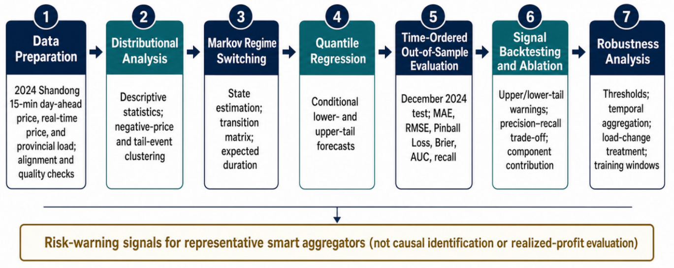
Figure 1 summarizes the empirical workflow adopted in this study.

1.4. Contributions and Scope

The primary contribution is methodological: this paper integrates Markov regime-switching, conditional quantile estimation, time-ordered out-of-sample testing, signal backtesting, component ablation, and robustness analysis in one reproducible risk-warning framework. The regime model characterizes persistence, the quantile model estimates asymmetric tail exposure, and the validation design tests whether those outputs remain useful outside the estimation sample. The Shandong application then demonstrates how the framework can be interpreted by smart aggregators operating in the day-ahead and real-time segments of an electricity spot market.

The current dataset contains day-ahead prices, real-time prices, medium- and long-term settlement-point prices, and provincial real-time load, but it does not include wind generation, photovoltaic generation, renewable forecast errors, interprovincial exchange, unit outages, reserve capacity, asset-level bids, or individual aggregator positions. Therefore, this paper does not claim to solve a full optimal dispatch or profit-maximizing trading problem for a specific aggregator. Instead, the conclusions are confined to spread regimes, tail risk, predictive associations, and signal interpretation observed under a high-renewable market background. Future 15 min or hourly wind and photovoltaic output, participant bids, flexible-resource availability, and forecast errors would allow the framework to be extended to explicit trading-strategy evaluation and to identification of the operational drivers of regime-transition probabilities and tail quantiles.

1.5. Paper Organization

The remainder of this paper is organized as follows. Section 2 introduces the background of the Shandong electricity spot market, the data sources, variable construction, regime-switching model, quantile regression model, out-of-sample forecasting design, and trading-signal interpretation for smart aggregators. Section 3 reports descriptive statistics, characteristics of negative prices and extreme spreads, regime-identification results, quantile effects, tail-risk measures, and forecasting performance. Section 4 discusses the interpretation boundary, distributional patterns, regime persistence, tail-risk forecasting, and risk-aware signal implications, and relates the findings to the existing literature. Section 5 summarizes the main conclusions, limitations, and future extensions.

2. Materials and Methods

The empirical design combines market-background interpretation, high-frequency spread modeling, tail-risk forecasting, and trading-signal interpretation. The current sample contains day-ahead prices, real-time prices, medium- and long-term settlement-point prices, and provincial load for Shandong at 15 min resolution in 2024. It does not include wind generation, photovoltaic generation, renewable forecast errors, interprovincial exchange, unit outages, reserve capacity, asset-level bids, flexible-resource availability, or realized aggregator positions. Accordingly, the analysis identifies distributional characteristics, regime persistence, conditional tail risk, and risk-aware signals in the Shandong day-ahead–real-time spread, but it does not interpret statistical associations as causal effects of renewable energy or as realized profits from a specific trading strategy.

All timestamps are processed in Beijing time, corresponding to Coordinated Universal Time plus eight hours (UTC+8). The main sample retains the 15 min frequency to avoid hourly aggregation masking short-term risks associated with negative prices, price spikes, and real-time imbalance settlement. Descriptive statistics, regime models, and quantile models report core results in Chinese yuan per megawatt-hour (CNY/MWh). To compare the marginal effects of different explanatory variables, continuous regressors may be standardized in regression estimation, while their economic meanings in original units are also reported in the results tables.

2.1. Shandong Electricity Spot Market Context

Shandong is selected because it combines a large and rapidly changing generation fleet, a mature provincial market architecture, formal spot-market operation during the sample year, and access to a complete 15 min market dataset for the sample year. By November 2024, new-energy and renewable capacity reached 106.426 GW and accounted for 46.90% of total installed capacity, slightly exceeding coal power at 46.88%; storage, natural gas, and waste-heat/other sources accounted for 2.63%, 0.57%, and 3.02%, respectively [22]. This coexistence of a still-substantial thermal fleet and a renewable fleet of comparable scale makes Shandong a useful stress test for distributional price-risk tools. The selection does not imply that renewable output is causally identified in the present price–load dataset.

The Shandong market links medium- and long-term transactions, the electricity spot market, ancillary services, and retail settlement [4,23]. At the end of 2023, participating supply-side entities included 153 directly dispatched public thermal units, 2 nuclear units, 564 renewable stations, 24 independent new-energy storage stations, 2 wind-plus-storage joint entities, and 3 local biomass plants; the user side included 101 retailers and 5 wholesale users [23]. Under the 2024 rules, the day-ahead and real-time segments use 96 settlement intervals per day, while system security constraints, interprovincial tie-line plans, reserve requirements, and updated load and renewable forecasts enter market operation [4]. These institutional features explain why a 15 min spread is relevant to smart-aggregator exposure management.

2.2. Data and Sample

The empirical dataset was provided by State Grid Shandong Electric Power Company for academic research under non-public data-access arrangements. The dataset is not publicly accessible. It covers 1 January–31 December 2024 (366 trading days), with 96 intervals of 15 min each per day and 35,136 observations. The fields are date, interval, real-time price, day-ahead price, medium- and long-term settlement-point price, and provincial load. Date and interval were merged into a unique Beijing-time timestamp, and the 24:00 observation was retained as the final interval of its trading day. The public market rules cited in this paper [4] are used only to describe the institutional setting and are not the source of the empirical price and load data. No wind, photovoltaic, outage, reserve, bid, asset-position, or aggregator-revenue series was included in the estimation sample.

Table 1. Current data fields, processing methods, and research uses.

Original Field	Frequency/Unit	Cleaning Procedure	Use in This Study
Date and interval	15 min; 96 intervals/day	Merged into Beijing-time timestamps; trading-day labels retained	Construct intraday intervals, months, workday indicators, and rolling forecasting windows
Real-time price	CNY/MWh	Negative prices and spikes retained; only verifiable entry errors checked	One dependent variable; used with the day-ahead price to construct the spread
Day-ahead price	CNY/MWh	Original prices retained; aligned with real-time prices at the same frequency	Expected price signal; spread benchmark; regression covariate
Medium- and long-term settlement-point price	CNY/MWh	Identical to the day-ahead price in the full sample; not separately included in the main model	Used as a data-consistency check; can be extended if independent medium- and long-term prices become available
Provincial load	MW	No missing values; construct 15 min load changes and check day-boundary jumps	Proxy for system demand and ramping pressure

Source: Authors’ compilation based on the non-public dataset provided by State Grid Shandong Electric Power Company.

summarizes the available fields, processing procedures, and research uses.

2.3. Data Quality and Preprocessing

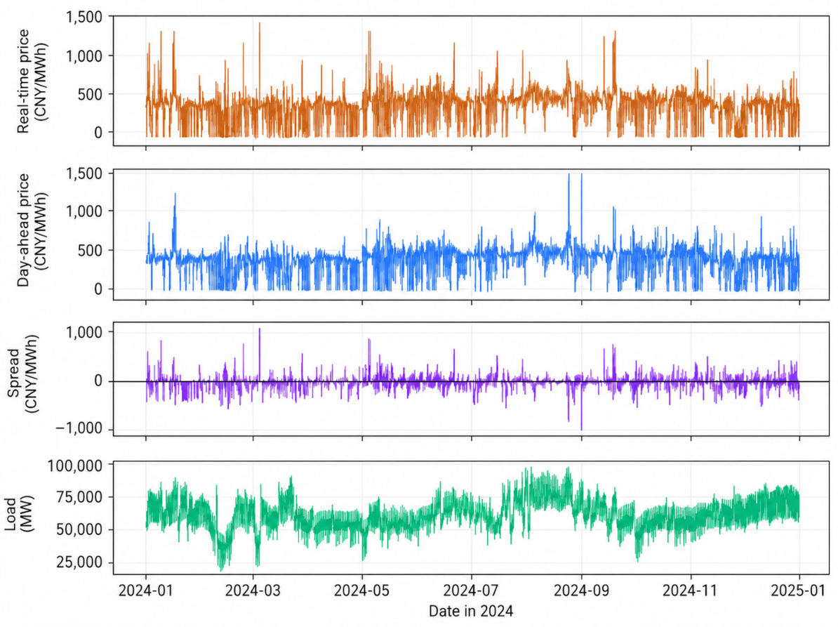
The data-quality check shows that real-time prices, day-ahead prices, medium- and long-term settlement-point prices, and provincial load contain no missing values, that timestamps are not duplicated, and that the trading-day–interval structure is complete. The mean real-time price is 306.90 CNY/MWh, with a standard deviation of 206.84 CNY/MWh, a minimum of −100 CNY/MWh, and a maximum of 1424.31 CNY/MWh. The mean day-ahead price is 314.40 CNY/MWh, with a standard deviation of 186.52 CNY/MWh, a minimum of −100 CNY/MWh, and a maximum of 1500 CNY/MWh. There are 4832 real-time negative-price intervals and 3757 day-ahead negative-price intervals, indicating that negative prices occur with sufficient empirical frequency in the sample and should not be removed as ordinary outliers.

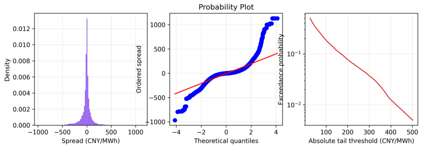
The spread defined as the real-time price minus the day-ahead price has a mean of −7.50 CNY/MWh and a median close to zero (−0.005 CNY/MWh), but its standard deviation reaches 114.08 CNY/MWh. The 1%, 5%, 95%, and 99% quantiles are −372.68, −196.84, 137.65, and 338.04 CNY/MWh, respectively, and the minimum and maximum values are −966.45 and 1132.61 CNY/MWh. These statistics suggest that the mean of the Shandong day-ahead–real-time price spread contains limited information, whereas the upper and lower tails better capture the imbalance-settlement exposure and trading-warning value faced by smart aggregators and other market participants.

The mean load is 63,003.29 MW, with a standard deviation of 10,692.70 MW and a maximum of 98,041.33 MW. The mean 15 min load change is close to zero, but the largest positive change is 32,733.09 MW and the largest negative change is −28,436.30 MW, suggesting that some day-boundary or recording points may contain jumps. The main sample does not mechanically delete price observations because of load jumps. Instead, three alternative treatments are considered in the robustness checks: removing or marking day-boundary load changes, winsorizing load changes at the 1% and 99% quantiles, and re-estimating the models using hourly aggregated data. This treatment preserves extreme prices as the object of analysis while avoiding the interpretation of potential recording issues as economic mechanisms.

Because high-frequency electricity price series exhibit pronounced intraday periodicity, serial correlation, and heteroskedasticity, this study does not treat the 35,136 intervals as independent and identically distributed observations. Statistical inference for means, quantiles, and regression results prioritizes standard errors clustered by trading day, Newey–West heteroskedasticity- and autocorrelation-consistent standard errors [24], or moving-block bootstrap methods [25]. For spikes, negative prices, and regime-transition results, this study reports event duration and continuous exposure length rather than only the number of independent time points.

2.4. Variable Construction

The core variable of this study is the day-ahead–real-time price spread, defined in Equation (1). A positive spread indicates that the real-time price exceeds the day-ahead price, so a participant that needs to purchase electricity in the real-time market may face higher costs, whereas a flexible resource that can reduce demand or inject energy may receive a stronger real-time signal. A negative spread indicates that the real-time price is lower than the day-ahead price, which may create low-price adjustment opportunities, but may also generate settlement risk for day-ahead positions. Around this core variable, this study constructs four groups of explanatory variables: price variables, load variables, calendar variables, and lagged-state variables. Real-time negative prices, extreme spreads, and load changes are defined in Equations (2)–(4).

Table 2. Definitions and economic meanings of core variables.

Variable	Definition	Unit/Form	Economic Meaning
Spreadt	PtRT − PtDA	CNY/MWh	Deviation between day-ahead expectations and real-time balancing; core measure of imbalance-settlement risk
NegRTt	I(PtRT < 0)	0/1 variable	Real-time negative-price event, used to identify low-price tails and negative-price regimes
Tailt+/Tailt−	I(Spreadt ≥ q0.95 or q0.99); I(Spreadt ≤ q0.05 or q0.01)	0/1 variable	Extreme positive- and negative-spread events, used for tail-risk modeling
Loadt	Provincial load	MW	Demand-side scale variable
ΔLoadt	Loadt − Loadt−1	MW/15 min	Proxy for short-term ramping pressure and real-time balancing pressure
Calendart	Month, interval, workday/weekend, and holiday indicators	Dummy variables	Control for seasonality, intraday structure, and institutional electricity-use differences
Lagt	Spreadt−1, Spreadt−96, NegRTt−1	Lagged terms	Capture mean reversion, daily-cycle memory, and event persistence

Source: Authors’ formulation.

defines the core variables and their economic meanings.

Notation and abbreviation convention. Subscript t denotes the 15 min interval; i and j index Markov states; τ denotes a quantile level; a hat denotes a forecast; superscripts + and − denote upper- and lower-tail events; DA and RT denote day-ahead and real-time, respectively; scalar variables are italicized, named operators and units are upright, and X_t denotes the covariate vector. Each symbol is defined at first use below Equations (1)–(13).

$${\mathit{Spread}}_t=P_t^{\mathit{RT}}-P_t^{\mathit{DA}}$$

(1)

where P_t^RT denotes the real-time price at time t, P_t^DA denotes the day-ahead price at time t, and Spread_t denotes the day-ahead–real-time price spread.

$${\mathit{NegRT}}_t=\mathrm{I}(P_t^{\mathit{RT}}< 0)$$

(2)

where I(·) is an indicator function. NegRT_t equals one when the real-time price is below zero and zero otherwise.

$${\mathit{Tail}}_t^{+}=\mathrm{I}({\mathit{Spread}}_t\ge q_{0.95}),{\mathit{Tail}}_t^{-}=\mathrm{I}({\mathit{Spread}}_t\le q_{0.05})$$

(3)

where q_0.95 and q_0.05 denote the 95th and 5th percentiles of the empirical spread distribution, respectively.

$${\mathsf{\Delta }\mathit{Load}}_t={\mathit{Load}}_t-{\mathit{Load}}_{t-1}$$

(4)

where Load_t denotes provincial load at time t, and ΔLoad_t denotes the change in load over adjacent 15 min intervals.

A future operational extension can incorporate outdoor air temperature and solar output at the same 15 min frequency. Temperature can enter through heating- and cooling-degree functions interacted with heating-season and intraday indicators, while measured and forecast photovoltaic output can enter separately so that solar-driven net-load variation is not conflated with temperature-sensitive thermal demand. Lagged temperature, forecast updates, and interaction terms can then be added to X_t and to time-varying transition probabilities. This would allow the model to distinguish weather-sensitive heating demand from solar-generation fluctuations, subject to out-of-sample and multicollinearity checks.

2.5. Distributional Analysis

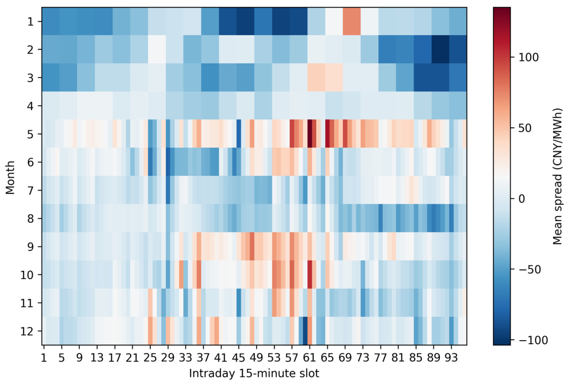
The descriptive analysis first reports the mean, standard deviation, minimum, maximum, and the 1%, 5%, 25%, 50%, 75%, 95%, and 99% quantiles of the real-time price, day-ahead price, load, load change, and spread. Given the common occurrence of spikes, negative prices, and heavy tails in electricity prices [10], this study compares not only means, but also the distribution of spreads using kernel density plots, box plots, quantile–quantile (Q–Q) plots, month-by-interval heatmaps, and tail exceedance probability curves. For negative-price and extreme-spread events, this study records their starting intervals, durations, inter-event times, monthly clustering, and intraday clustering to distinguish isolated spikes from persistent regimes.

The purpose of this part is to distinguish a mean close to zero from significant tail risk. In the current data, the correlations between load and real-time and day-ahead prices are 0.418 and 0.444, respectively, whereas the correlation between load and the spread is only 0.032, and the correlation between load change and the spread is 0.051. This fact suggests that simple linear correlations may be insufficient to explain spread risk. A more appropriate approach is to characterize the spread under different market regimes and at different quantiles from the perspectives of regime-switching and conditional distributions.

2.6. Regime-Switching Model

To identify whether the Shandong day-ahead–real-time spread is generated by different mechanisms, such as normal conditions, small deviations, negative or low-price regimes, and spike or high-price regimes, this study adopts a Markov regime-switching model. Hamilton’s regime-switching framework characterizes probabilistic switching among unobserved states in time series [11]. In electricity price research, Huisman and Mahieu apply the idea of regime jumps to explain price spikes and institutional changes [26], providing a direct methodological basis for the analysis of spread regimes in this paper.

The basic specification of the regime-switching model is shown in Equation (5), the state-transition probability is given in Equation (6), and the expected regime duration is defined in Equation (7).

$${\mathit{Spread}}_t={\mu }_{z_t}+{\phi }_{z_t}{\mathit{Spread}}_{t-1}+{\beta \prime }_{z_t}{X}_t+{\epsilon }_{t,z_t}$$

(5)

where z_t denotes the unobserved market regime, X_t is the vector of explanatory variables, and μ, φ, β, and ε denote the regime-dependent intercept, autoregressive coefficient, covariate coefficient, and error term, respectively.

$$p_{\mathit{ij}}=\mathrm{Pr}(z_t=j |z_{t-1}=i)$$

(6)

where p_ij denotes the conditional probability that the market regime switches from i to j.

$$D_i={\displaystyle \frac{1}{1 - p_{\mathit{ii}}}}$$

(7)

where D_i denotes the expected duration of regime i, and p_ii denotes the probability that regime i remains unchanged.

The selection of the number of regimes K is based on the Akaike information criterion (AIC), the Bayesian information criterion (BIC), regime interpretability, convergence stability, multi-start reproducibility, and out-of-sample performance. This study begins with two- and three-state models. The two-state model distinguishes normal conditions from extreme deviations, whereas the three-state model separates negative-deviation, near-zero, and positive-deviation states. The final specification reports regime-specific means, variances, sample shares, expected durations, the full row-stochastic transition matrix, and smoothed state probabilities.

2.7. Quantile Regression Model and Tail-Risk Measures

The regime model answers the question of which market regime the spread occupies, whereas quantile regression addresses how explanatory variables affect different parts of the spread distribution. The quantile regression proposed by Koenker and Bassett directly estimates different quantiles of the conditional distribution [12], and Koenker and Hallock further explain its interpretive value in economics [13]. In electricity price research, quantile regression has been used to characterize the asymmetric effects of renewable energy on price levels and volatility [14] and to estimate the tail behavior of electricity price distributions [15].

This study estimates conditional quantile models for τ ∈ {0.05, 0.10, 0.25, 0.50, 0.75, 0.90, 0.95}, as specified in Equation (8). If the coefficients differ markedly between the upper and lower tails, mean regression cannot adequately describe the imbalance risks faced by market participants. Model results are displayed using coefficient-path plots, and coefficient differences between the 5% and 95% quantiles and between the 10% and 90% quantiles are examined.

$$\begin{gathered} Q_{\tau }({\mathit{Spread}}_t|X_t) = {\beta }_0\left(\tau ) + {\beta }_1\right(\tau )P_t^{\mathit{DA}}+{\beta }_2(\tau ){\mathit{Load}}_t + \\ {\beta }_3\left(\tau \right){\mathsf{\Delta }\mathit{Load}}_t+{\beta }_4\left(\tau \right){\mathit{Spread}}_{t-1}+\gamma {\left(\tau \right)}^{\prime }{\mathit{Calendar}}_t \end{gathered}$$

(8)

where τ denotes the quantile level, and Calendar_t denotes calendar variables such as month, intraday interval, and weekend indicators.

The tail-risk indicator is based primarily on conditional Value-at-Risk (VaR), as defined in Equation (9). For positive spread risk, τ = 0.95 or 0.99 is of particular interest; for negative spread risk, τ = 0.05 or 0.01 is relevant. The present empirical design reports conditional quantile forecasts rather than Expected Shortfall estimates, because stable tail-mean estimation would require additional validation beyond the current price–load dataset. The validity of conditional quantile forecasts can be assessed using Christoffersen’s interval-forecast backtesting method [27], and quantile loss follows the logic of strictly consistent scoring rules [28].

$${\mathit{VaR}}_{\tau ,t}=Q_{\tau }\left({\mathit{Spread}}_t\right|X_t)$$

(9)

where VaR_τ,t denotes the conditional risk value at time t for quantile level τ.

2.8. Out-of-Sample Evaluation

To avoid information leakage caused by randomly shuffling high-frequency time series, this study constructs the out-of-sample evaluation in chronological order. The baseline design uses January to September 2024 as the initial training set, October to November as the model-selection and tuning window, and December as the final test set. Rolling-window and expanding-window designs are also used for robustness checks. Each forecast uses only information available before the forecast time, and intraday dummy variables and month variables are treated as predetermined information.

The baseline models include the historical mean, empirical quantiles grouped by month and intraday interval, a linear autoregressive model, and an autoregressive integrated moving average (ARIMA)-type benchmark implemented through the seasonal autoregressive integrated moving average with exogenous regressors (SARIMAX) specification SARIMAX(1,0,1). Point forecasts are evaluated by mean absolute error (MAE) and root mean squared error (RMSE), defined in Equations (10) and (11), respectively. Quantile forecasts use Pinball Loss (Equation (12)). Extreme-event probability forecasts use the Brier Score (Equation (13)), the area under the receiver operating characteristic curve (AUC), recall, and the precision–recall area under the curve (PR AUC). Signal backtesting also reports precision, false-alarm rate, warning share, conditional mean spread, and tail exposure for a representative 1 MWh position. Forecast-loss differences are tested with the Diebold–Mariano procedure [29] or moving-block bootstrap intervals.

$$\mathrm{MAE}={\displaystyle \frac{1}{n}}{\displaystyle \sum _{t=1}^n}|y_t-{\widehat{\mathrm{y}}}_t|$$

(10)

where y_t is the realized spread, ŷ_t is the point forecast, and n is the evaluation sample size.

$$\mathrm{RMSE}=\sqrt{{\displaystyle \frac{1}{n}}{\displaystyle \sum _{t=1}^n}{(y_t-{\widehat{\mathrm{y}}}_t)}^2}$$

(11)

where y_t is the realized spread, ŷ_t is the point forecast, and n is the evaluation sample size.

$$L_{\tau }\left(y_t,{\widehat{q}}_t\right)=\left(\tau -\mathrm{I}\left(y_t<{\widehat{q}}_t\right)\right)\left(y_t-{\widehat{q}}_t\right)$$

(12)

where ${\widehat{q}}_t$ is the quantile forecast, and I(·) is an indicator function.

$$\mathrm{BS}={\displaystyle \frac{1}{n}}{\displaystyle \sum _{t=1}^n}{\left({\widehat{p}}_t-o_t\right)}^2$$

(13)

where ${\widehat{p}}_t$ is the predicted probability of an extreme event, and o_t is the 0/1 observation indicating whether the event occurs.

2.9. Trading-Signal Interpretation for Smart Aggregators

The empirical models in this paper are designed as a risk-aware signal framework rather than as a complete optimal-dispatch model. For a representative smart aggregator participating in day-ahead and real-time electricity spot markets, the relevant decision problem is to determine whether the current price-spread environment supports routine position adjustment, requires tail-risk warning, or calls for tighter exposure control. The model outputs are therefore interpreted as four signal components: the smoothed probability of each spread regime, the expected duration of the current regime, the conditional upper- and lower-tail quantiles of the spread, and the predicted probability of extreme spread events. In this interpretation, regime probabilities describe persistence and exposure conditions, whereas quantile forecasts serve as direct tail-event triggers. The subsequent backtesting exercise evaluates whether these signals can identify realized upper- and lower-tail spread events in the December 2024 test window.

The signal interpretation follows the economic meaning of the spread. A negative-deviation signal is activated when the probability of the negative-spread regime is high or when the lower-tail quantile falls below the historical risk threshold; this indicates low-price or negative-price exposure, and warns against relying on average-price forecasts. A positive-deviation signal is activated when the probability of the positive-spread regime or the upper-tail quantile is high; this warns of real-time procurement cost, scarcity exposure, or high-price imbalance risk. A persistence signal is obtained from the Markov transition probabilities and expected regime duration, indicating whether the current state is likely to last for several 15 min settlement intervals. These signals can support day-ahead position revision, real-time exposure limits, flexible-load activation, storage charging/discharging timing, and demand-response preparation, while the present study does not claim to optimize the physical dispatch of any specific aggregator portfolio.

2.10. Robustness, Reproducibility, and Artificial Intelligence Disclosure

The robustness checks include five categories. First, the number of regimes K, the error distribution, and initial values are changed to assess whether the regime interpretation is stable. Second, the extreme-spread thresholds are changed from 5%/95% to 1%/99%, and alternative definitions of negative-price events are compared. Third, the 15 min main sample is compared with an hourly aggregated sample to determine whether high-frequency noise drives the conclusions. Fourth, the training-window length and test month are changed to examine out-of-sample performance. Fifth, raw, marked, winsorized, and trimmed treatments of load jumps are used to assess whether the direction and significance of load-related variables remain stable.

To meet the reproducibility requirements of Energies, this study fixes and stores the data-cleaning scripts, variable dictionary, model-estimation code, random seeds, software versions, and the automatic workflow used to generate all tables and figures. Data processing and statistical analysis were conducted using Python (Python Software Foundation, Wilmington, DE, USA), and figures were generated using Matplotlib version 3.10.3 (Matplotlib Development Team). Future extensions can incorporate wind generation, photovoltaic generation, renewable forecast errors, interprovincial exchange, unit constraints, reserve capacity, participant bids, flexible-resource availability, and realized aggregator positions. Such extensions would allow mechanism identification and explicit trading-strategy evaluation, whereas the present manuscript remains limited to statistical relationships based on price–load data, risk-aware signal interpretation, and out-of-sample warning performance. The use of generative artificial intelligence (AI) is disclosed at the end of the manuscript. All conclusions, data processing, tables, and figures have been checked by the authors.

3. Results

This section reports empirical results based on 15 min data from the Shandong electricity spot market for 2024. All statistics, model parameters, and forecasting metrics are derived from the generated experimental tables and figures. The interpretation is confined to distributional patterns, regime persistence, tail-risk prediction, and signal performance.

3.1. Empirical Distribution and Stylized Facts

Table 3. Descriptive statistics of real-time prices, day-ahead prices, day-ahead–real-time spreads, provincial load, and load changes.

Var.	N	Mean	Std.	Min.	q01	q05	q25	Med.	q75	q95	q99	Max.
RT	35,136	306.90	206.84	−100.00	−85.000	−80.000	201.28	354.53	424.68	570.07	795.76	1424.31
DA	35,136	314.40	186.52	−100.00	−100.00	−80.000	244.92	358.54	423.26	546.25	697.27	1500.00
Spread	35,136	−7.497	114.08	−966.45	−372.68	−196.84	−29.980	−0.0050	23.185	137.65	338.04	1132.61
Load	35,136	63,003.29	10,692.70	23,308.27	35,850.98	46,929.03	55,750.36	62,362.00	69,998.38	80,934.13	88,921.35	98,041.33
ΔLoad	35,136	0.1098	947.55	−28,436.30	−1864.42	−1247.82	−546.32	−91.545	547.87	1419.97	2135.06	32,733.09

Source: Authors’ calculations based on non-public data provided by State Grid Shandong Electric Power Company. Note: N = sample size; Std. = standard deviation; Min. = minimum; Med. = median; Max. = maximum; q01, q05, q25, q75, q95, and q99 denote the corresponding empirical quantiles.

and Figure 2 describe the empirical distribution after the data construction and quality checks reported in Section 2.2 and Section 2.3. Real-time and day-ahead prices move together over much of the year, but their difference remains centered near zero only in typical intervals and displays intermittent positive and negative spikes. Figure 2 presents the price, spread, and provincial-load time series.

The spread, defined as the real-time price minus the day-ahead price, has a mean of −7.50 CNY/MWh, a median of −0.005 CNY/MWh, and a standard deviation of 114.08 CNY/MWh. Its minimum and maximum are −966.45 and 1132.61 CNY/MWh, respectively (Table 3). The 5% and 95% quantiles are −196.84 and 137.65 CNY/MWh, and the 1% and 99% quantiles are −372.68 and 338.04 CNY/MWh (Table 3), respectively. This quantile structure indicates that, although the median spread is close to zero, the upper and lower tails are wide, and the mean alone is insufficient to summarize the imbalance risk faced by market participants. The same pattern is also visible in the density plot, Q–Q plot, and tail exceedance probability curve (Figure 2, Figure 3 and Figure 4).

The empirical distribution is also characterized by recurrent negative prices and large load movements. Real-time negative prices occur in 4832 intervals (13.75%), compared with 3757 day-ahead negative-price intervals (10.69%). The 15 min load-change distribution is wide, but load itself has only a weak contemporaneous correlation with the spread, supporting the subsequent use of lagged, calendar, regime, and conditional-quantile information rather than a purely contemporaneous mean relationship.

3.2. Intraday and Monthly Clustering of Negative Prices and Extreme Spreads

The monthly distribution indicates substantial heterogeneity in real-time negative prices. February records the largest number of real-time negative-price intervals, with 860 observations, accounting for 30.89% of all observations in that month. March has 684 intervals, accounting for 22.98%, whereas August has the lowest number, with 68 intervals and a share of 2.28% (

Table 4. Core statistics of negative-price and extreme day-ahead–real-time spread events.

Panel	Item	Count/Obs.	Share	Mean Spread/Threshold
Panel A: Events	RT negative	4832	13.75%	-
Panel A: Events	DA negative	3757	10.69%	-
Panel A: Events	Spread ≤ q0.05	1757	5.00%	-
Panel A: Events	Spread ≥ q0.95	1757	5.00%	-
Panel A: Events	Spread ≤ q0.01	352	1.00%	-
Panel A: Events	Spread ≥ q0.99	352	1.00%	-
Panel B: Monthly RT negative	Month 2	860	30.89%	−32.62
Panel B: Monthly RT negative	Month 3	684	22.98%	−27.18
Panel B: Monthly RT negative	Month 11	520	18.06%	−3.44
Panel B: Monthly RT negative	Month 4	492	17.08%	−7.02
Panel C: Intraday RT negative	Slot 49	163	44.54%	−6.89
Panel C: Intraday RT negative	Slot 50	163	44.54%	−3.80
Panel C: Intraday RT negative	Slot 51	163	44.54%	−11.97
Panel C: Intraday RT negative	Slot 52	163	44.54%	−17.37

Source: Authors’ calculations based on non-public data provided by State Grid Shandong Electric Power Company.

). The month-by-96 intraday-interval heatmap in Figure 3 further shows that spread levels are not uniformly distributed, but instead form concentrated regions along both the monthly and intraday dimensions.

Real-time negative prices also exhibit pronounced intraday clustering. The intraday interval with the highest number of negative prices is the 49th 15 min interval, with 163 real-time negative-price observations, accounting for 44.54% of the observations in that interval over the year (Table 4). The four intervals with the largest number of negative-price observations are the 49th, 50th, 51st, and 52nd 15 min intervals, each with 163 observations. By contrast, the four intervals with the fewest observations are the 72nd, 71st, 70th, and 69th intervals, each with only one real-time negative-price observation (Table 4).

After extreme spreads are defined using empirical quantiles, the upper and lower tails have symmetric counts but different economic meanings. The 5% negative-tail threshold is −196.84 CNY/MWh and the 95% positive-tail threshold is 137.65 CNY/MWh. Observations below the 5% threshold and above the 95% threshold each number 1757, accounting for 5.00% of the sample (Table 4). Under the stricter 1%/99% thresholds, the negative-tail threshold is −372.68 CNY/MWh and the positive-tail threshold is 338.04 CNY/MWh, with 352 observations in each tail and a share of 1.00% (Table 4). Based on the average intraday spread, the 61st interval has the highest mean value, 43.72 CNY/MWh, whereas the 93rd interval has the lowest mean value, −42.81 CNY/MWh (Table 4; Figure 3).

3.3. Regime-Switching Results

The regime-switching model comparison shows that both specifications converged. The two-state model has a log-likelihood of −190,435.719, an AIC of 380,883.438, and a BIC of 380,934.240. The three-state model has a log-likelihood of −184,737.311, an AIC of 369,498.622, and a BIC of 369,600.225 (

Table 5. Comparison of Markov regime-switching models, regime parameters, and transition matrix.

Panel	Model/State/from State	Log-Likelihood/Mean/to State 0	AIC/Variance/to State 1	BIC/Share/to State 2	Converged/Expected Duration
Model comparison	markov_2_state	−190,435.719	380,883.438	380,934.240	Yes
Model comparison	markov_3_state	−184,737.311	369,498.622	369,600.225	Yes
3-state parameters	State 0	−44.12	56,589.68	20.40%/0.939	4.11 h
3-state parameters	State 1	−1.29	87.23	35.27%/0.933	3.74 h
3-state parameters	State 2	4.42	2455.76	44.33%/0.932	3.69 h
Transition matrix	From State 0	0.9392	0.0522	0.0086	Row sum = 1.0000
Transition matrix	From State 1	0.0411	0.9332	0.0256	Row sum = 0.9999
Transition matrix	From State 2	0.0140	0.0538	0.9322	Row sum = 1.0000

Source: Authors’ calculations based on non-public data provided by State Grid Shandong Electric Power Company. Note: AIC and BIC are reported to three decimal places; transition probabilities are reported to four decimal places. Displayed row sums may differ from unity only because of rounding. Expected durations are calculated as 1/(1 − p_ii) using the unrounded diagonal probabilities from the fitted model.

). These values are identical to the rechecked estimation output and are reported to three decimal places. The lower AIC and BIC and the economic separation of negative-deviation, near-zero, and positive-deviation states support the three-state specification.

The three-state model identifies three regimes with distinct means and variances. Regime 0 accounts for 20.40% of the sample, with a mean spread of −44.12 CNY/MWh and a variance of 56,589.68. Regime 1 accounts for 35.27% of the sample, with a mean of −1.29 CNY/MWh and a variance of 87.23. Regime 2 accounts for 44.33% of the sample, with a mean of 4.42 CNY/MWh and a variance of 2455.76 (Table 5). Accordingly, Regime 0 can be interpreted as a negative-deviation and high-volatility regime, Regime 1 as a near-zero and low-volatility regime, and Regime 2 as a regime with a slightly positive mean and higher volatility than Regime 1. Figure 5 shows the evolution of the smoothed probabilities of each regime and marks real-time negative-price and extreme-spread intervals.

The rechecked row-stochastic transition matrix is P = [[0.9392, 0.0522, 0.0086], [0.0411, 0.9332, 0.0256], [0.0140, 0.0538, 0.9322]], where each row is the origin state and each column is the destination state (Table 5). The diagonal probabilities correspond to expected durations of 16.447, 14.977, and 14.754 intervals, or 4.112, 3.744, and 3.689 h. The durations were calculated from the unrounded diagonal probabilities; probabilities shown in Table 5 are rounded to four decimals.

3.4. Quantile Regression and Tail Risk

The quantile regression uses standardized day-ahead price, provincial load, 15 min load change, lagged spreads, month dummy variables, intraday-interval dummy variables, and weekend dummy variables to explain the distribution of the spread. Figure 6 presents the coefficient paths of the core variables across quantiles, and

Table 6. Tail-quantile results for core variables in quantile regression (coef., p-value).

Variable	τ = 0.05	τ = 0.10	τ = 0.90	τ = 0.95	Main Pattern
Day-ahead price (standardized)	−0.701 (0.000)	−0.345 (0.000)	−1.245 (0.000)	−1.897 (0.000)	Negative in both tails
Provincial load (standardized)	0.431 (0.000)	0.189 (0.008)	0.116 (0.298)	0.103 (0.646)	Stronger statistical evidence at lower quantiles
15 min load change (standardized)	−3.547 (0.000)	−2.049 (0.000)	−2.635 (0.000)	−4.834 (0.000)	Negative at tail quantiles
Spread lag 1 (standardized)	112.706 (0.000)	113.175 (0.000)	112.491 (0.000)	112.112 (0.000)	Short-term persistence is most prominent
Spread lag 96 (standardized)	0.324 (0.000)	0.280 (0.000)	0.229 (0.000)	0.269 (0.030)	Daily-cycle memory is weaker but positive

Source: Authors’ calculations based on non-public data provided by State Grid Shandong Electric Power Company.

reports coefficients, standard errors, confidence intervals, and p-values. This subsection focuses on the 5%, 10%, 90%, and 95% tail quantiles.

The coefficients of the day-ahead price are negative at all four tail quantiles. At τ = 0.05, 0.10, 0.90, and 0.95, the coefficients are −0.701, −0.345, −1.245, and −1.897, respectively, with p-values below conventional significance levels (Table 6). This indicates that, after controlling for lagged spreads, load, and calendar factors, the day-ahead price has a negative marginal relationship with both tails of the spread distribution, as also shown by the coefficient path in Figure 6.

Provincial load has positive coefficients at lower quantiles and smaller coefficients at higher quantiles. At τ = 0.05 and τ = 0.10, the coefficients are 0.431 and 0.189, with p-values of 0.0000 and 0.0083, respectively. At τ = 0.90 and τ = 0.95, the coefficients are 0.116 and 0.103, with p-values of 0.2976 and 0.6455 (Table 6), respectively. Thus, the load variable has stronger statistical evidence in the lower tail, whereas estimates in the upper tail are less stable than those at lower quantiles (Figure 6).

The 15 min load-change variable is negative at all four tail quantiles, with the largest absolute value at the 95% quantile. At τ = 0.05, 0.10, 0.90, and 0.95, its coefficients are −3.547, −2.049, −2.635, and −4.834, respectively (Table 6). By contrast, the coefficient of the first lag of the spread remains close to 112 across the tail quantiles: 112.706, 113.175, 112.491, and 112.112 at τ = 0.05, 0.10, 0.90, and 0.95, respectively (Table 6). The coefficient of the 96th lag of the spread is smaller but positive, taking values of 0.324, 0.280, 0.229, and 0.269 at the four tail quantiles (Table 6). These results indicate that the short-term persistence of the spread itself is the most prominent statistical feature of conditional tail risk (Figure 6).

3.5. Out-of-Sample Forecasting Performance

The out-of-sample forecasting exercise is split chronologically. The training set runs from 2024-01-01 00:15 to 2024-10-01 00:00, and contains 26,304 observations. The validation set runs from 2024-10-01 00:15 to 2024-12-01 00:00, and contains 5856 observations. The test set covers December 2024, and contains 2976 observations (

Table 7. Out-of-sample forecasting performance in December 2024.

Model	MAE	RMSE	Pinball	Brier	AUC	Recall	PR AUC
Quantile reg.	24.015	49.673	7.021	0.0237	0.9314	0.7317	0.7724
Linear + state	24.310	46.745	7.312	0.0241	0.9515	0.6646	0.7358
Linear reg.	24.365	46.794	7.316	0.0240	0.9522	0.6890	0.7374
Hist. mean	55.535	88.312	14.180	0.0521	0.5000	0.0000	0.5276
SARIMAX(1,0,1)	55.711	88.095	18.563	0.0542	0.5123	0.0000	0.5282
Month-slot	56.204	87.979	13.479	0.0508	0.6616	0.0000	0.1393

Source: Authors’ calculations based on non-public data provided by State Grid Shandong Electric Power Company. Note: Quantile reg. = quantile regression; Linear + state = linear regression with lagged state probabilities; Linear reg. = linear regression; Hist. mean = historical mean; SARIMAX = seasonal autoregressive integrated moving average with exogenous regressors.

). Extreme positive-spread events are defined using the 95% quantile of the training set, with a threshold of 135.22 CNY/MWh (Table 7). Figure 7 displays rolling forecasting losses and extreme-event probabilities during the test period.

For point-forecast metrics, quantile regression yields the lowest MAE, 24.015. Its RMSE is 49.673, and its average Pinball Loss is 7.021 (Table 7). The model with the lowest RMSE is the linear model with lagged state probabilities, with an RMSE of 46.745; the RMSE of linear regression is 46.794 (Table 7). Thus, quantile regression performs best in terms of mean absolute error and quantile loss, whereas the linear model augmented with state probabilities performs better under squared-error criteria. For a smart aggregator, this distinction is important: squared-error criteria favor average point accuracy, whereas quantile loss is more directly connected to conservative tail-risk control.

Compared with simple baselines, regression-based models have substantially lower forecast errors. The MAE and RMSE of the historical mean model are 55.535 and 88.312, respectively, and those of the month-slot empirical model are 56.204 and 87.979. The MAE and RMSE of SARIMAX(1,0,1) are 55.711 and 88.095 (Table 7), respectively. For quantile forecasts, the Pinball Loss of quantile regression is 7.021, lower than 14.180 for the historical mean, 13.479 for the month-slot empirical model, and 18.563 for SARIMAX(1,0,1) (Table 7).

For extreme positive-spread event prediction, linear regression has an AUC of 0.952, the linear model with lagged state probabilities has an AUC of 0.951, and quantile regression has an AUC of 0.931 (Table 7). However, quantile regression achieves the highest extreme-event recall, 0.732, whereas the recall rates of linear regression and the linear model with lagged state probabilities are 0.689 and 0.665, respectively (Table 7). This indicates that different models trade off ranking ability, recall, and loss functions differently. In trading-signal applications, a model with higher recall may be preferred when missing an extreme positive-spread event is more costly than issuing a false warning, while a model with lower RMSE may be preferred for routine position adjustment. Figure 7 provides graphical evidence of the evolution of event probabilities during the test period.

3.6. Trading-Signal Backtesting and Component Ablation

To examine whether the forecasts can be used as risk-aware trading signals rather than only as statistical predictions, this study conducts a December 2024 backtesting exercise (

Table 8. Backtesting results for risk-aware trading signals in December 2024.

Signal	Tail	Warnings	Events	Precision	Recall	False Alarm	Tail Exposure	Lead
Upper quantile	Upper	360	164	0.397	0.872	0.077	28.63	15 min
Lower quantile	Lower	134	82	0.515	0.841	0.022	40.26	15 min
Negative-regime	Lower	564	82	0.145	1.000	0.167	10.47	15 min

Source: Authors’ calculations based on non-public data provided by State Grid Shandong Electric Power Company.

). Positive-tail events are defined using the 95% quantile of the training-set spread distribution, 135.22 CNY/MWh, and negative-tail events are defined using the 5% quantile, −212.64 CNY/MWh. An upper-tail quantile signal is activated when the predicted 95% conditional quantile exceeds the positive-tail threshold, and a lower-tail quantile signal is activated when the predicted 5% conditional quantile falls below the negative-tail threshold. Regime-probability signals are identified according to the economically ordered regime means, and are used mainly to interpret persistence and continuous exposure.

The backtesting results show that quantile signals provide useful but imperfect tail-event warnings. The upper-tail signal issues 360 warnings and captures 143 of 164 positive-tail events, yielding recall of 0.872 and precision of 0.397. Thus, 217 warnings are not followed by a realized upper-tail event, and 60.3% of issued upper-tail warnings are unnecessary when judged by this binary threshold. The reported 7.7% false-alarm rate uses all non-event intervals as its denominator and should not be confused with one minus precision. This trade-off is acceptable only when the cost of missing a severe positive spread exceeds the cost of preparing flexibility unnecessarily. In less risk-averse applications, the warning threshold should be raised or calibrated to a user-specified false-warning budget. The lower-tail signal issues 134 warnings, with precision of 0.515, recall of 0.841, and a 2.2% false-alarm rate. Regime probabilities remain more appropriate for persistence and exposure interpretation than for standalone event triggering.

The component ablation further clarifies why the proposed signal framework works. Removing lagged spread variables increases MAE from 24.015 to 54.278 CNY/MWh, RMSE from 49.673 to 85.750 CNY/MWh, and Pinball Loss from 7.021 to 14.736 (

Table 9. Component ablation of the quantile-based trading-signal model.

Model	MAE	RMSE	Pinball	Brier	AUC	Recall	PR AUC
Full QR signal	24.015	49.673	7.021	0.0237	0.931	0.732	0.726
Without lagged spread	54.278	85.750	14.736	0.0503	0.698	0.000	0.175
Without calendar controls	24.603	51.288	7.718	0.0255	0.933	0.720	0.702
Without load variables	24.011	49.669	7.380	0.0244	0.931	0.726	0.723

Source: Authors’ calculations based on non-public data provided by State Grid Shandong Electric Power Company.

). Removing calendar controls also worsens MAE, RMSE, Pinball Loss, Brier Score, and PR AUC, although the change is smaller than the effect of removing lagged spreads. Removing load variables has little effect on MAE and RMSE, but increases Pinball Loss from 7.021 to 7.380, suggesting that load-related variables are more useful for tail-risk calibration than for median point prediction. These findings support the interpretation that short-term spread persistence is the dominant predictive component, while calendar and load information improve the calibration of risk-aware tail signals.

For statistical comparison, the absolute-error loss difference between quantile regression and simple baselines is evaluated using a Newey–West-adjusted Diebold–Mariano statistic with 96 lags. Quantile regression reduces absolute-error loss by 31.52 CNY/MWh relative to the historical mean benchmark and by 32.19 CNY/MWh relative to the month-slot empirical benchmark, with t-statistics of 8.29 and 8.65, respectively. The difference between quantile regression and the linear models is much smaller, which is consistent with Table 7: regression-based models are all effective for average prediction, whereas the quantile model is more useful for conservative tail-risk warning.

3.7. Robustness Checks

First, the threshold-substitution test shows that, under the 5%/95% thresholds, the lower-tail and upper-tail observations each number 1757, with a share of 5.00% in each tail. Under the 1%/99% thresholds, the lower-tail and upper-tail observations each number 352, with a share of 1.00% (

Table 10. Robustness-check results.

Panel	Setting	N/Count	MAE/Mean/Coef.	RMSE/Std./p	Tail/Pinball
Threshold	5%/95%	1757	Lower = −196.84	Upper = 137.65	Share = 5.00%
Threshold	1%/99%	352	Lower = −372.68	Upper = 338.04	Share = 1.00%
Frequency	15 min	35,136	−7.50	114.08	RT neg = 13.75%
Frequency	hourly	8785	−7.50	108.50	RT neg = 13.22%
Δ Load	raw	35,040	0.175	p = 0.558	R2 = 0.853
Δ Load	winsor_1_99	35,040	0.170	p = 0.546	R2 = 0.853
Δ Load	drop_abs_delta_top1pct	34,688	0.117	p = 0.673	R2 = 0.854
Window	Jan-Aug	23,328	24.998	48.080	q95 = 6.537
Window	Jan-Sep	26,208	24.960	47.894	q95 = 6.484
Window	Jan-Oct	29,184	24.777	47.451	q95 = 6.368
Window	Jan-Nov	32,064	24.365	46.794	q95 = 6.203

Source: Authors’ calculations based on non-public data provided by State Grid Shandong Electric Power Company. Note: Slash-separated column labels report the metric applicable to each panel, including count or sample size, MAE or mean or coefficient, RMSE or standard deviation or p-value, and tail Pinball Loss or the reported auxiliary statistic.

). The corresponding thresholds are −196.84 and 137.65 CNY/MWh under the 5%/95% scheme, and −372.68 and 338.04 CNY/MWh under the 1%/99% scheme (Table 10), respectively.

Second, the frequency-aggregation test shows that the 15 min sample contains 35,136 observations, with a mean spread of −7.50 CNY/MWh and a standard deviation of 114.08 CNY/MWh. The hourly aggregated sample contains 8785 observations, with a mean spread of −7.50 CNY/MWh and a standard deviation of 108.50 CNY/MWh (Table 10). After hourly aggregation, the 5% and 95% spread quantiles are −186.88 and 127.20 CNY/MWh, respectively, and the share of real-time negative prices is 13.22%. The corresponding real-time negative-price share in the 15 min sample is 13.75% (Table 10).

Third, alternative treatments of load changes do not alter the basic conclusions from the robustness ordinary least squares (OLS) regressions. Under the raw treatment, the coefficient of ΔLoad_t is 0.175, with a p-value of 0.558. Under 1%/99% winsorization, the coefficient is 0.170, with a p-value of 0.546. After dropping the top 1% of observations in absolute load change, the coefficient is 0.117, with a p-value of 0.673 (Table 10). The R² values under the three treatments are 0.853, 0.853, and 0.854, respectively (Table 10).

Finally, the training-window robustness test shows that, as the training window expands from January–August to January–November, test-set MAE declines from 24.998 to 24.365, RMSE declines from 48.080 to 46.794, and the 95% quantile Pinball Loss declines from 6.537 to 6.203 (Table 10). Among the four training windows, the January–November window yields the lowest MAE, indicating that, under the current out-of-sample design, adding training data closer to the test period helps improve forecasting performance (Table 10).

4. Discussion

4.1. Main Findings and Comparison with the Existing Literature

The empirical results show that the average level of the Shandong day-ahead–real-time spread does not fully summarize market risk. The median spread is close to zero, but the two tails of the distribution exhibit clear deviations, and real-time negative prices and extreme spreads show monthly and intraday clustering (Table 3 and Table 4; Figure 2 and Figure 3). This pattern is consistent with the literature on negative electricity prices, price spikes, and renewable energy price effects: under high renewable energy penetration, price risk is more likely to appear as concentrated tail exposure in the conditional distribution than as a one-directional shift in the mean. For smart aggregators, these tail events are not only statistical observations, but also potential signals for real-time exposure control and flexible-resource activation. The signal backtesting results further show that upper- and lower-tail quantile signals can identify most realized tail events in the December test set (Table 8).

It is important to emphasize that this study uses price, load, calendar, and lagged-state variables, but does not include wind output, photovoltaic output, forecast-error variables, asset-level bid curves, or realized aggregator positions. Therefore, the analysis concerns the statistical associations, regime characteristics, tail risk, and signal interpretation observed under high renewable energy penetration, rather than a causal identification of the effect of renewable output on spread movements or a complete profit-maximizing trading model. Compared with the existing literature, the contribution of this paper lies in placing the day-ahead–real-time spread within a regime-switching and conditional-quantile framework, and then evaluating whether the resulting probabilities and tail forecasts can function as risk-aware trading signals.

4.2. Interpretation Boundary and Market-Signal Meaning

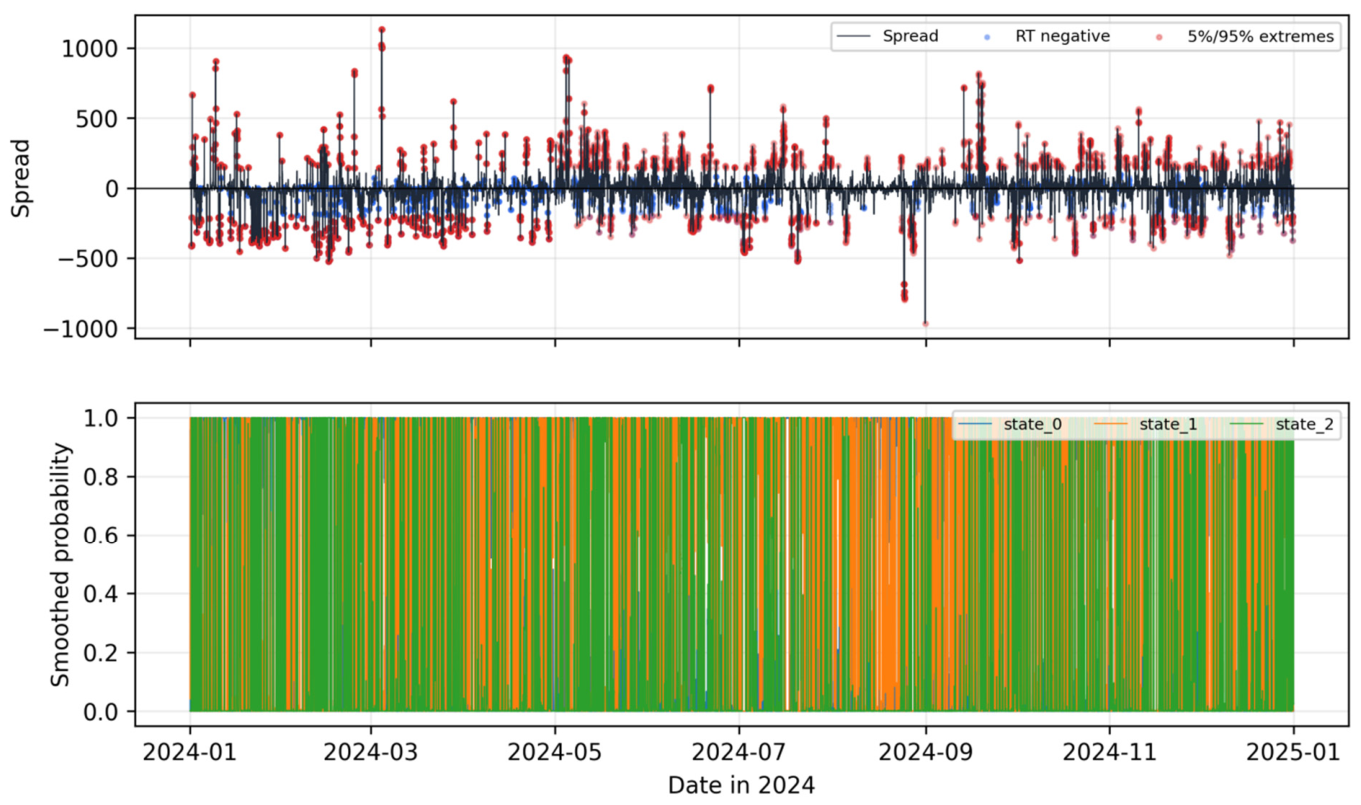
The three-state Markov model classifies the spread into three regimes: a negative-deviation high-volatility regime, a near-zero low-volatility regime, and a positive-deviation regime. The three-state model also performs better than the two-state model according to information criteria (Table 5; Figure 5). This result suggests that the day-ahead–real-time spread does not fluctuate randomly around a single mean, but may switch among different risk regimes. Because the available data contain only prices, load, calendar variables, and lagged spread information, these regimes should be interpreted as distributional and predictive states rather than as evidence of specific causal mechanisms such as renewable-output shocks, unit constraints, reserve scarcity, or bidding behavior.

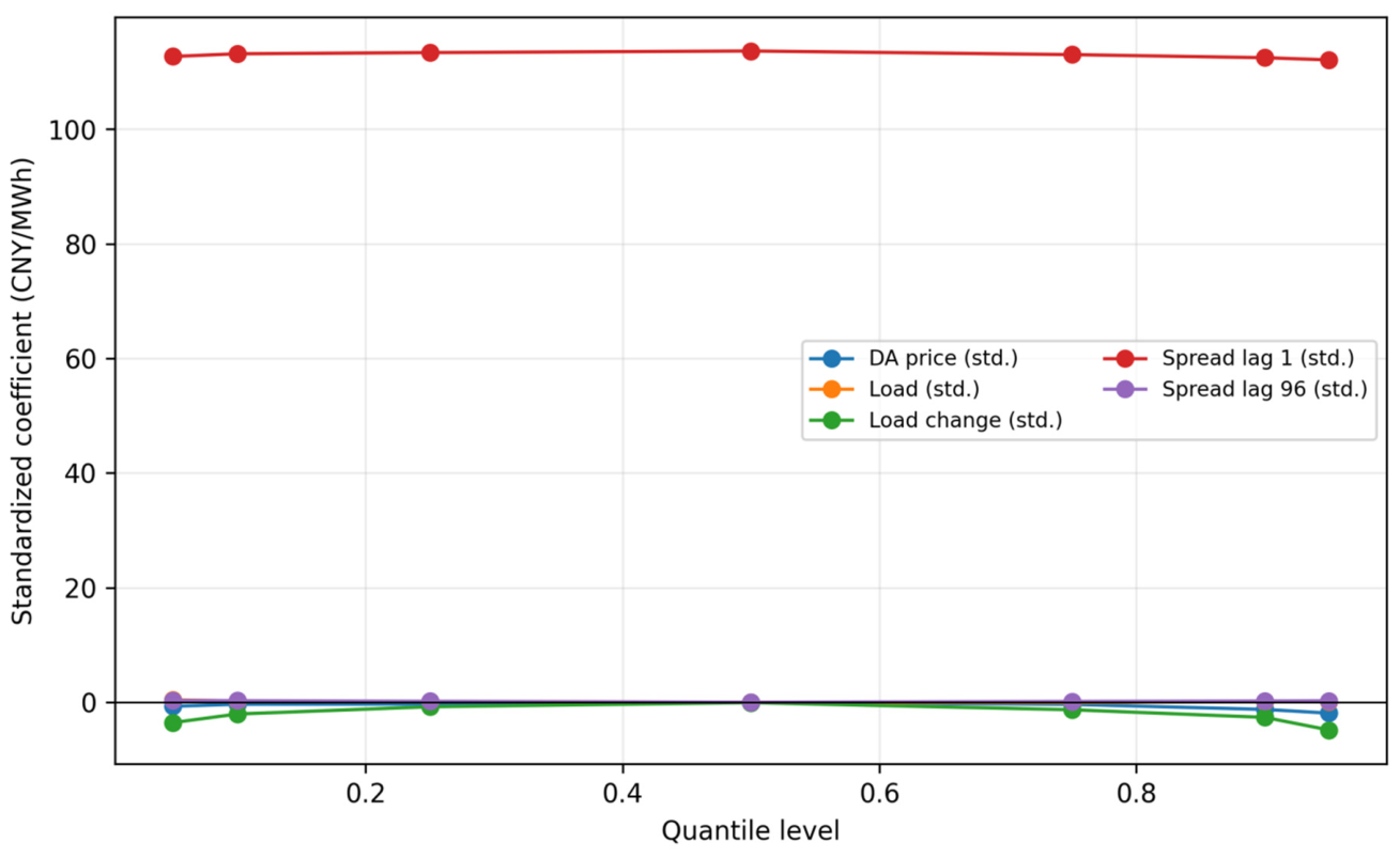
Regime persistence further indicates that the relevant object of risk management is not an isolated 15 min interval, but a price regime characterized by continuous exposure. The quantile-regression results also show that day-ahead prices, load, 15 min load changes, and lagged spreads have different marginal relationships across the lower and upper tail quantiles (Table 6; Figure 6). These findings support an interpretation centered on distributional patterns, short-term inertia, intraday structure, and the location of the conditional distribution. They do not establish causal effects of renewable generation, outages, reserves, bids, or participant positions, because those system and participant variables are not observed in the current dataset.

4.3. Implications for Smart Aggregator Trading

For smart aggregators, the regime of the day-ahead–real-time spread can be used to identify windows of cross-time-scale trading risk. When the market is in a negative-deviation regime, real-time prices are lower than day-ahead expectations, which may indicate low-price adjustment opportunities for flexible demand, but may also reduce the settlement value of previously scheduled supply positions. When the market is in a positive-deviation environment, real-time procurement and imbalance settlement become more costly, so aggregators with controllable load, storage, or demand-response resources may reduce real-time exposure or activate flexibility. The backtesting results suggest that tail-quantile signals are more suitable for event triggering, whereas regime probabilities are more useful for interpreting persistence, continuous exposure, and the likely duration of a risk state. Thus, the proposed framework should be read as a two-layer warning system: quantile forecasts trigger tail-risk alerts, while regime probabilities describe whether the exposure is likely to persist. In both cases, bidding revisions, position adjustment, and risk-limit management should not rely solely on average spreads.

The upper-tail precision–recall trade-off also limits operational interpretation. High recall reduces missed scarcity warnings, but can trigger avoidable re-optimization, reserve procurement, storage repositioning, or demand-response preparation. An aggregator should therefore choose the alert threshold by comparing the expected cost of a missed extreme event with the cost of an unnecessary response, and should report both precision and recall rather than presenting recall alone.

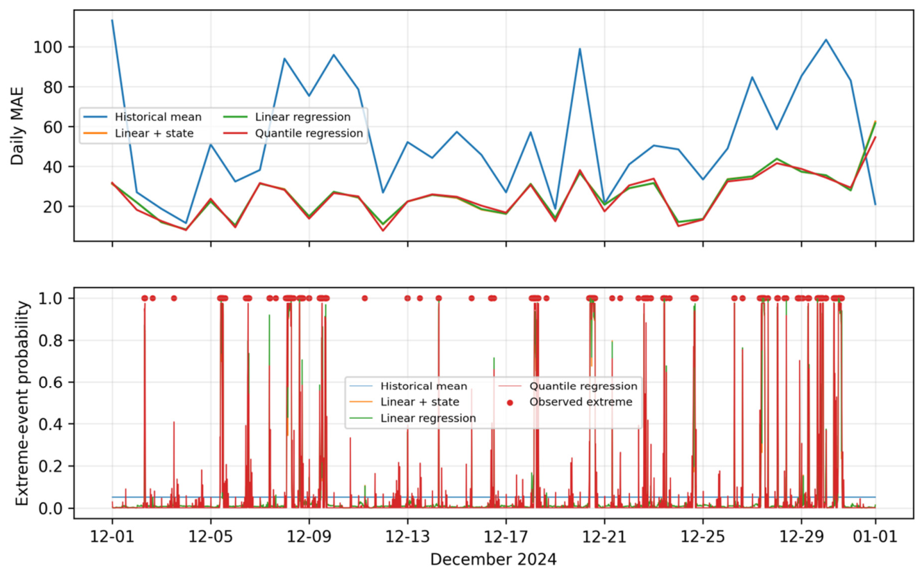
The persistence of spread regimes provides risk-constraint information for trading-signal design. If exposure-control decisions are made only from single-interval spread signals, aggregators may underestimate the volatility associated with continuous negative prices or persistent positive deviations. Combining state probabilities with quantile forecasts can better distinguish temporary noise from persistent spread signals. The out-of-sample forecasting and ablation results show that models differ in their advantages across MAE, RMSE, Pinball Loss, extreme-event recall, and component contribution (Table 7, Table 8 and Table 9; Figure 7). Smart aggregators should therefore select forecasting models according to specific objectives: routine day-ahead position adjustment may emphasize MAE or RMSE, tail-risk warning may emphasize Pinball Loss and recall, and portfolio risk control may emphasize Brier Score, AUC, regime duration, and false-alarm rate.

4.4. Regulatory and Market Design Implications

From a regulatory perspective, the monthly and intraday clustering of negative prices and extreme spreads indicates that monitoring mechanisms should extend beyond average prices to tail events, regime duration, and conditional risk indicators. Reporting only average prices or the number of isolated extreme events may underestimate the impact of continuous exposure on participants’ financial risk and market stability. Regulators may use negative-price frequency, extreme-spread thresholds, state probabilities, and quantile forecasts as complementary indicators for monitoring electricity spot market operation.

From the perspective of market design, the findings support further attention to flexible resources, storage, demand response, smart aggregation, and forecast-deviation management under a high-renewable market background. However, policy interpretation should remain limited to the observed distributional patterns and warning indicators. Future work incorporating wind generation, photovoltaic generation, forecast errors, interprovincial exchange, unit availability, reserve capacity, market bids, network constraints, and participant-level trading data could identify the operational drivers of regime-switching and tail risk more directly, and extend the signal framework into explicit strategy evaluation.

4.5. Limitations and Future Research

This study has several limitations. First, the sample covers only 15 min market data from Shandong in 2024, and the results should not be directly extrapolated to other provinces, other years, or different market-rule stages. Second, the current data do not include system-operation variables such as wind output, photovoltaic output, renewable forecast errors, interprovincial exchange, unit outages, reserve capacity, and network constraints. Third, the data do not include asset-level bids, flexible-resource availability, charging/discharging quantities, or realized smart-aggregator positions. Therefore, the conclusions mainly reflect statistical associations, regime identification, predictive performance, and risk-aware signal interpretation, and cannot be interpreted as causal effects of renewable output or as realized profits from an optimal trading strategy. The proposed signals should be interpreted as pre-dispatch risk-warning indicators rather than complete bidding, dispatch, or portfolio-optimization strategies.

Future research can incorporate wind generation, photovoltaic generation, renewable forecast errors, unit availability, reserve capacity, market bids, flexible-resource availability, and realized aggregator positions within the same reproducible framework to analyze the drivers of regime-transition probabilities, negative-price events, and tail quantiles. It can also compare different provincial markets or longer samples to test the robustness of the regime–quantile framework across market environments. If participant-level bidding and position data become available, the risk-identification framework developed in this paper can be extended from trading-signal analysis to explicit trading-strategy backtesting and market-design simulation.

5. Conclusions

This study constructs the day-ahead–real-time price spread as real-time price minus day-ahead price using non-public 2024 15 min day-ahead prices, real-time prices, and provincial load data provided by State Grid Shandong Electric Power Company for the Shandong electricity spot market. The empirical analysis leads to five conclusions.

First, the average spread is not sufficient for assessing market risk. The spread has a mean of −7.50 CNY/MWh and a median of −0.005 CNY/MWh, while the 5% and 95% quantiles are −196.84 and 137.65 CNY/MWh and the 1% and 99% quantiles are −372.68 and 338.04 CNY/MWh, respectively. Real-time negative prices and extreme spreads also exhibit clear monthly and intraday clustering. Second, the three-state Markov model identifies negative-deviation high-volatility, near-zero low-volatility, and positive-deviation regimes, with diagonal transition probabilities above 0.932 and expected durations of approximately 3.69–4.11 h. Third, quantile regression shows that day-ahead prices, load, 15 min load changes, and lagged spreads have different marginal relationships across the lower and upper tails, and the first lag of the spread is the dominant predictor of conditional tail behavior. Fourth, the out-of-sample test shows that the upper-tail quantile signal reaches a recall of 0.872 for positive extreme spreads, and the lower-tail quantile signal reaches a recall of 0.841 for negative extreme spreads. Fifth, the ablation study indicates that lagged spreads are the most important predictive component, since removing them increases MAE from 24.015 to 54.278 CNY/MWh and Pinball Loss from 7.021 to 14.736.

For smart aggregators, these results should be used as risk-aware signals and warning indicators rather than as evidence of realized trading profits or optimal dispatch decisions. State probabilities and quantile forecasts can support pre-dispatch warning, real-time exposure control, demand-response preparation, flexible-resource activation, and tail-risk monitoring. For other market participants and regulators, negative-price frequency, extreme-spread thresholds, regime duration, and tail forecasts provide complementary indicators beyond average-price monitoring.

The conclusions should be interpreted within the boundary of the available data. Because the current sample does not include wind generation, photovoltaic generation, renewable forecast errors, interprovincial exchange, unit availability, outage counts, reserve capacity, market bids, asset-level flexibility, or realized aggregator positions, the identified spread regimes and tail risks cannot be interpreted as causal outcomes of renewable-output changes or as the profitability of a specific trading strategy. Future research can incorporate these system-operation and participant-level variables, together with longer samples, to identify mechanisms more directly and to extend the present warning signals into risk-constrained bidding, dispatch, or trading-optimization models.